Morphometric Traits of Old Blue (Andinoacara rivulatus) in Their Native Habitat and Aquaculture Environments: A Study of the Quevedo Region, Ecuador

1. Introduction

The Old Blue (Andinoacara rivulatus), a charismatic species of cichlid native to the tropical waters of South America [1] has attracted significant attention due to its vibrant coloration, unique behavior, and potential value in aquaculture [2,3]. Its ecological importance and economic potential have led to its cultivation in fish farms in several regions, including the Quevedo area of Ecuador [4,5]. However, the transition from natural to captive environments can potentially influence the morphometric characteristics of this species, raising questions about potential phenotypic changes and their underlying mechanisms.

Morphometric traits, which encompass measurements of size, shapes, and proportions, serve as essential indicators of an organism’s adaptation to its environment [6,7] .These traits are influenced by several factors, including genetic background, ecological conditions, and resource availability [8,9] Therefore, a thorough analysis of morphometric traits in wild and aquaculture populations of Old Blue natives is crucial to understanding the potential impacts of captivity on their phenotypic expression.

Research of (A. rivulatus) in both its native and aquaculture habitats in Ecuador is of paramount importance due to the notable lack of comprehensive scientific studies and findings on this intriguing cichlid species [10]. Despite their captivating appearance and potential economic value, there is a significant knowledge gap about the morphometric traits and adaptations of ancient native blue populations under varying ecological conditions.

It is a fish with a large defined head, of the same proportions as the trunk and tail, the adult male has a hump behind the forehead that characterizes it, the dorsal fin is large, covers an adipose area, and its pectoral fins are large, unlike the fin. Generally, we find a pair of pectoral and pelvic fins, one on each side of the body, and a single dorsal and caudal fin, located in the dorsal and ventral midline, the mouth with teeth at the end of the snout. Symmetrical tail homofence rounded, belongs to the family Cichlidæ, indicating that its scales are cycloid, small, and oval, with growth rings [11]

The paucity of empirical data on its response to captive environments hinders our understanding of how this species might exhibit phenotypic changes in controlled environments. By addressing this research gap, we can not only improve our understanding of the species’ adaptive potential but also pave the way for informed decision-making in terms of conservation strategies and sustainable aquaculture practices. Consequently, this study strives to bridge the existing gap in knowledge and provide a fundamental basis for future research, yielding insights that are crucial for the effective management and conservation of ancient native blue populations both in their natural habitat and in aquaculture contexts.

This study investigates the morphometric characteristics of ancient native blue populations, comparing individuals from their native habitat with those raised on fish farms within the Quevedo region of Ecuador. By examining how these traits vary in these contrasting environments, we seek to shed light on the potential phenotypic plasticity and adaptive responses that might arise from differences in environmental conditions.

We hypothesize that there will be perceptible differences in morphometric traits between ancient native blue populations inhabiting their natural environment and those residing in fish farms. Specifically, we expect that certain traits related to body size, shape, and performance may exhibit variations between the two environments. By conducting a detailed comparative analysis, this study aims to contribute to a better understanding of how the morphology of A. rivulatus responds to different ecological contexts, thus providing insights into the species’ potential for practical practices in sustainable aquaculture while preserving their natural characteristics.

2. Materials and Methods

2.1. Area of Study

The research focused on three distinct locations within the Quevedo region of Ecuador, each of which exhibits different altitudinal, climatic, and soil characteristics. These sites, namely Buena Fe, El Empalme, and Mocache, were selected to comprehensively evaluate the morphometric traits of A. rivulatus both in its natural habitat and in aquaculture environments. These diverse ecological scenarios were chosen to elucidate the impact of environmental variables on the morphometric traits of Old Blue natives, both in their natural and aquaculture environments. The inclusion of locations with different altitudes, climates, and soil compositions ensures a comprehensive understanding of the adaptation and growth patterns of species in different habitats within the Quevedo region.

Buena Fe (0°40’16.7”S; 79°24’52.2” W), is located at a moderate altitude (120 - 162 m.a.s.l.), and experiences a warm humid climate with temperatures ranging between 23 and 32°C. The region enjoys favorable climatic conditions marked by satisfactory humidity levels and is subject to hot and cold winds. In addition, El Empalme (0°54’41.9”S; 79°39’53.1”W) is located at a lower altitude (73-115 m.a.s.l.) and has a humid climate, characterized by continuous rains from the foothills of the coastal mountain range. The region experiences a monsoon climate (AM) with consistently high temperatures throughout the year, ranging from 26 to 30 °C. The topography of El Empalme is diverse, with mounds, hills, and elevations of the orographic system, hosting large rivers such as the Daule, the Balzar and the Peripa or Puntilla.

Finally, Mocache (1°14’37.1”S 79°30’38.5”W) is located at a relatively lower altitude (40-75 m.a.s.l.), it has a tropical savannah climate with temperatures ranging between 24 and 28°C. The region experiences distinct dry and wet seasons, contributing to an average annual temperature of 26°C. Semi-humid megathermal tropical climate, covering a large part of the canton and characterized by a prominent rainy peak and a well-defined dry season with rainfall ranging between 500 and 1000 mm.

2.2. Experimental Design

The morphometric characteristics of the species A. rivulatus were studied concerning 3 factors: reproduction systems (wild and fish farms), geographical localities (Buena Fe, El Empalme, and Mocache), and sex (male and female) with three replicates and with a complete three-factor design. There are 36 representative specimens per breeding system of 200 to 400 g each.

The species were captured by artisanal fishing with nets, their weights were recorded and individualized with OHAUS digital scales capacity 5 kg (±0.01 g) to standardize the weights of the adult individuals in each experimental area. The research was carried out in three localities or zones for the capture of the native species A. rivulatus in the wild: 1) Canton Buena Fe: Pico de Pato landfill, belonging to the Baba power plant (reservoir dam 1) located in Los Angeles, whose geographical coordinates are: 0°40’16.7”S 79°24’52.2”W; 2) El Empalme: Las Margaritas Enclosure, located via El Empalme-Manabí, on the Peripa River, of the Daule-Peripa Dam, with geographical coordinates: 0°54’41.9”S 79°39’53.1”W and 3) Mocache Canton: Estero Achiote, with coordinates: 1°14’37.1”S 79°30’38.5”W, belonging to the Quevedo River, via Mocache-Vinces. To obtain native species, A. rivulatus was collected in captivity in three fish farms: 1) “La Rivera” via Buena Fe; 2) swimming pools via El Empalme-Pichincha, and 3) Hacienda “San Marcos”, via Mocache-Vinces.

2.3. Morphometric Measurements

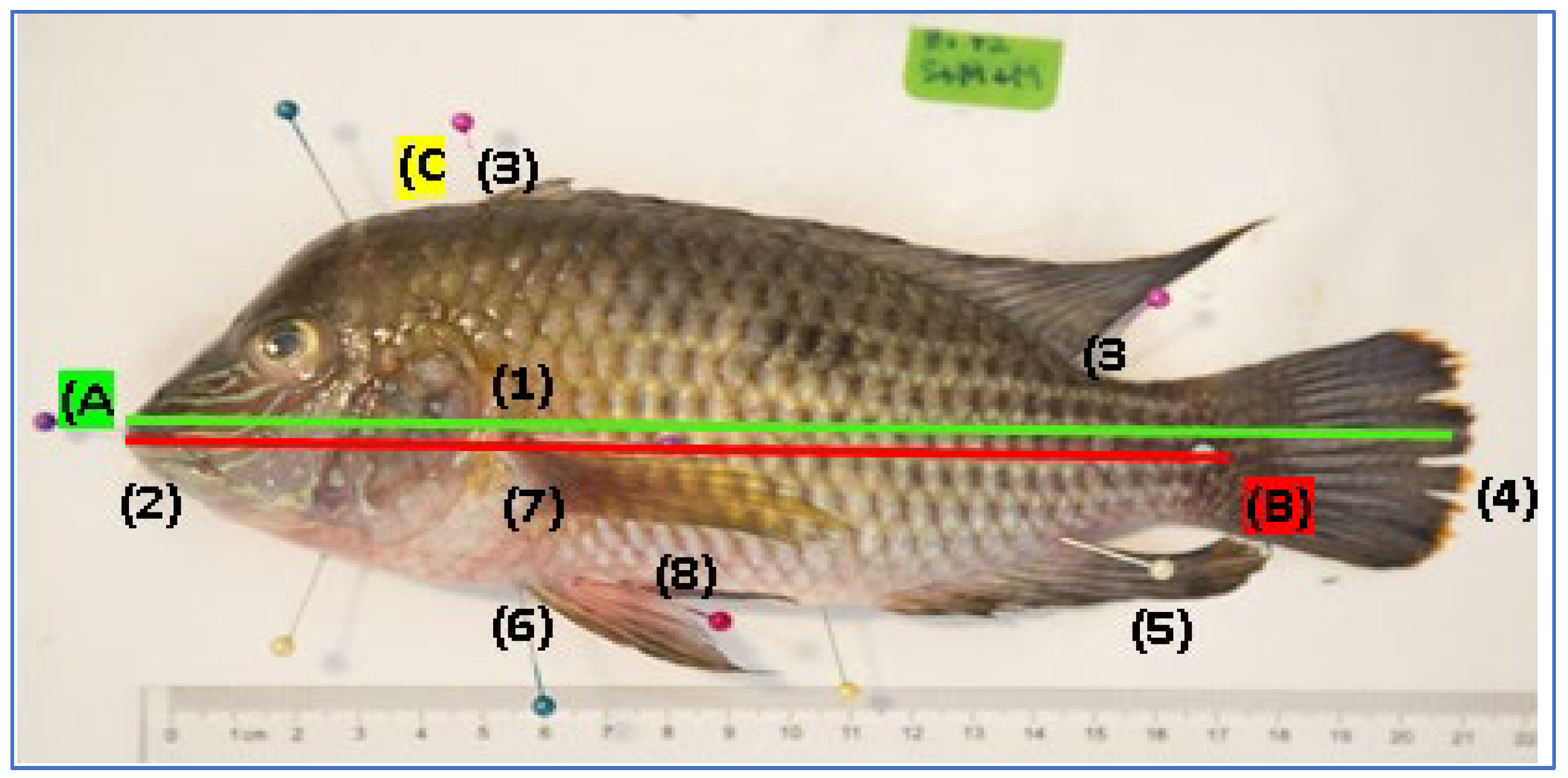
The morphometric evaluation of the specimens of A. rivulatus encompassed a complete set of 10 measurements in centimeters, adhering to the established standards proposed by [12] (Figure 1). Total length (A), from the mouth to the tip where the caudal fin ends; Standard length (B), from the mouth to the beginning of the caudal fin; The ventral dorsal length (C) is identified vertically, located in the highest area of the fish, usually at the beginning of the dorsal fin; Head length (1), measured horizontally, from the beginning of the mouth to the end of the gills; Length of the muzzle (2), to the end of the corner of the muzzle; Dorsal fin length (3), the length of the fin measured at its base; Caudal fin length (4), measured horizontally from the end of the standard length to the end of the fin; Fin length (5), from the beginning at the base of the fin to the tip where the fin ends; Pelvic fin length (6), starts at the base of the fish’s body where the fin begins, to the tip of the fin; Length of the pectoral fin (7), Ventral fin (8), its measurement begins at the base of the fin, where the body of the fish culminates.

Measurements were made using an ichthyometer (Pentair FMB2, USA), placing the fish horizontally on a flat surface. Simultaneously, fin measurements were made with a 40 cm diameter ruler on the same base. Sex determination was based on external characteristics and data for each species were diligently recorded during all instances of sampling.

To capture precise anatomical detail, pins were employed at anatomical landmarks on each specimen during measurements. Individuals with curvatures were straightened with needles. The high-resolution photographs were acquired with a Canon EOS 5D Mark III professional digital camera with a 24-105mm lens, placing the specimen consistently on the left side. Camera height considerations were considered, ensuring consistency across all images. Subsequently, the quantification of surfaces using AutoCAD (AutoCAD^®2020) was performed.

2.3. Experimental Weight and Yield Measurements of A. rivulatus

Total weight (1), corresponds to the weight of the whole fish freshly caught; Weight of gutted fish (2), fish open in the abdomen without viscera; Weight of fillet with skin (3), fish without head, scales, fins, viscera and skeleton; Yield of gutted fish (4), calculation of the weight of gutted fish over the total weight per hundred; Fillet yield (5), calculation of the weight of the fillet with skin on the total weight per hundred.

Weighing of the scale (6), separation of all fish scales and weighing; Fin weight (7), separation and weighing of dorsal, pectoral, caudal and pelvic fins; Weight of the head (8), from the mouth to the end of the gills; The weight of the viscera (9) includes the organs and gills of the fish removed by the weight of the gutted fish; Skeleton weight (10), skeleton weight, by separating the fillet, head and other by-products; By-products (11), calculation of the total weight of all by-products over the percentage by total weight.

2.4. Data Analysis

In data normalization, logarithmic transformation and data scaling were performed using mean centering. In version 4.0.2 of the R software (R Core Team, 2023). The logarithmic transformation with a base of 10 is obtained using the “glog” function [13]. For data scaling, mean centering calculates the average of each variable and subtracts it from each data point, resulting in a dataset in which the average of each variable is centered around zero.

The dataset matrix comprises 16 variables and n=36 observations represented in two groups of fish farming, wild (n=18) and farmed (n=18). Each row in the matrix represents a specific sample of points, while each column represents different variables. The variables are TW = Total Weight, GFW = Weight of Gutted Fish, GFY = Yield of Gutted Fish, FSW = Weight of Fillet with Skin, FY = Fillet Yield, FW = Weight of Balance, FINW = Fin Weight, HW = Head Weight, VW = Viscera Weight, SW = Skeleton Weight, SUBY = By-product Yield, TL = Total Length, SL= Standard Length, DVL= Rear Ventral Length, HL=Head Length, ML=Muzzle Length.

2.5. Analysis of Variance

This research used Analysis of Variance (ANOVA) as a statistical framework, executed using Infostat software version 2015 [14]. After ANOVA, Tukey’s test was used to make comparisons of means and significance levels were set at p<0.05. ANOVA was used to discern significant differences between the various levels of categorical variables, including reproductive systems, geographic locations, and sex. This analytical approach facilitates a comprehensive understanding of the influence of these factors on the morphometry of A. rivulatus. The utilization of this software, a well-established statistical analysis tool ensures a rigorous calculation and reliable results according to the designated parameters. Post hoc analysis was performed using Tukey’s test, a widely recognized method for comparing pairwise means. This allowed for the identification of specific variations or similarities between the groups, which contributed to a nuanced interpretation of the morphometric data.

2.6. Comparison of Fish Farming Groups Using Supervised Analyses

In this study, the application of supervised analysis using orthogonal least squares discriminant analysis (OPLS-DA) was used to reduce the dimensionality of the dataset of high-dimensional variables using “ropls” in R [15]. The aim was to create a robust and easily interpretable model that could effectively identify the primary characteristics of fish responsible for differentiation between fish farming groups (wild and farmed). The analysis was performed by modeling the class groups (wild and farmed) as the response variable and the fish variables as predictors. The OPLS-DA algorithm then extracted the latent variables that best discriminate between the two groups of classes, while orthogonalizing the remaining systematic variations [15]. By analyzing the Variable Importance in Projection (VIP) >1 obtained from the OPLS-DA model [16]. The main characteristics of fish that contribute to the separation of fish groups (wild and farmed) were identified. The 20 permutations were used to validate the performance of the OPLS-DA model. For the quality criteria, the R²Y (goodness-of-fit parameter) and Q² (predictive capacity parameter) criteria were chosen > 0.50 [17].

2.7. Exploring the Multivariate ROC Curve Using the Random Forest

Algorithm

After selecting the variables with VIP greater than 1, they underwent a multivariate exploratory analysis of the ROC curve. The objective of the analysis is to evaluate the performance of the models created through the automatic selection of fish variables through random forests (FR) [18]. ROC curves are generated by Monte Carlo cross-validation (MCCV) using balanced subsampling. In each MCCV, 2/3 of the samples are used to assess the importance of fish variables, and the remaining 1/3 is used to validate the models created in the first step [19]. The area under the ROC curve (AUC) quantifies this relationship so that a model is considered acceptable if the AUC ≥ 0.7, excellent if the AUC ≥0.8, and outstanding if the AUC ≥ 0.9. The “pROC” package and the “random Forest” function were used in R [20].

Research manuscripts reporting large datasets that are deposited in a publicly available database should specify where the data have been deposited and provide the relevant accession numbers. If the accession numbers have not yet been obtained at the time of submission, please state that they will be provided during review. They must be provided prior to publication.

Interventionary studies involving animals or humans, and other studies that require ethical approval, must list the authority that provided approval and the corresponding ethical approval code.

In this section, where applicable, authors are required to disclose details of how generative artificial intelligence (GenAI) has been used in this paper (e.g., to generate text, data, or graphics, or to assist in study design, data collection, analysis, or interpretation). The use of GenAI for superficial text editing (e.g., grammar, spelling, punctuation, and formatting) does not need to be declared

3. Results

This section may be divided by subheadings. It should provide a concise and precise description of the experimental results, their interpretation, as well as the experimental conclusions that can be drawn.

3.1. Analysis of Variance

The morphometric measurements reveal significant differences between Old Blue specimens from fish farms and their wild counterparts (Table 1). In fish farm conditions, Old Blue exhibited a significantly greater total length (25.04 ± 0.69) compared to their wild counterparts (23.21 ± 1.04) (p< 0.000). A similar pattern is observed in standard length, dorsoventral length, and head length, where fish farm individuals consistently displayed larger dimensions than the wild population (p < 0.000, p= 0.001, p= 0.006, respectively). Interestingly, the muzzle length did not exhibit a statistically significant difference between fish farms and wild individuals (p=0.124). This may suggest that specific morphological traits are influenced by the rearing system, while others remain relatively consistent between the two environments.

The morphometric analysis of Old Blue specimens across different zones in the Quevedo Region reveals notable variations in certain key traits (Table 1). Total length, standard length, dorsum-ventral length, and head length exhibit distinct patterns across the zones, with statistical significance observed in some instances. In terms of total length, individuals from Buena Fe (24.43 ± 1.26) and Mocache (24.03 ± 2.11) demonstrate comparable lengths, while those from El Empalme (23.90 ± 0.97) differ slightly, albeit not significantly (p= 0.174). Standard length, on the other hand, displays a significant difference among zones (p= 0.009), with individuals from El Empalme (19.98 ± 2,74) exhibiting greater lengths compared to those from Buena Fe (19.33 ± 0.98) and Mocache (19.19 ± 1.55). Dorsum-ventral length also reveals significant differences across zones (p= 0.000), with individuals from Buena Fe (8.64 ± 0.91) displaying larger dimensions compared to those from El Empalme (7.78 ± 0.42) and Mocache (7.93 ± 0.90). Conversely, head length does not exhibit statistically significant differences among zones (p= 0.123). Muzzle length, likewise, does not show significant differences among the three zones (p= 0.887). This suggests that the variation in this morphometric trait may not be influenced by the specific environmental conditions in these zones.

This study reveals pronounced sexual dimorphism in the morphometric traits of Old Blue, highlighting distinctions between males and females. Regarding total length, males exhibit a significantly larger size (24.44 ± 2.48) compared to females (23.80 ± 0.53) with a p-value of 0.0112. A similar trend is observed in standard length, where males (20.06 ± 2.88) surpass females (18.94 ± 0.60) significantly (p < 0.0001). Dorsoventral length also displays sexual dimorphism, with males (8.35 ± 1.14) showing larger dimensions compared to females (7.89 ± 1.10) (p= 0.0031). Contrastingly, head length does not demonstrate a statistically significant difference between sexes (p=0.1889), suggesting a level of similarity in this morphometric trait. Similarly, muzzle length does not exhibit significant sexual dimorphism (p= 0.5548).

Table 2 shows the average values of weights and yields expressed as percentages for various anatomical parts of A. rivulatus obtained from wild farming and farming systems. Comparison between wild specimens from the wild-caught fish factory and those from fish farms provides valuable information on morphometric traits and performance metrics in different environments within the Quevedo region, Ecuador.

The total weight of wild-caught fish was recorded at 260.64 ± 33.42 g, which constitutes the reference value, while farmed specimens exhibited a slightly higher weight of 334.39±23.98 g, indicating a notable increase in the size of farmed fish. This weight difference was consistently observed in several anatomical components, such as gutted fish, viscera, fins, scales, head, skeleton, and skin-on fillet, corroborating the increased overall growth and development of the farmed specimens.

Yield metrics, expressed as percentage yields, further highlight the efficiency of farm farming. The yield of gutted fish for wild specimens was 78.94%, while farmed specimens exhibited a higher yield of 80.77%, suggesting a more favorable anatomical composition in the latter. Similar trends were observed for other anatomical components, with farmed specimens consistently outperforming their wild counterparts in terms of yield percentages.

In addition, examination of skeletal weight highlights the impact of farming systems on the inedible part of fish. Farmed specimens demonstrate significantly higher body weight (101.18 ± 12.15 g) compared to wild specimens (63.91 ± 15.16 g), emphasizing the potential influence of controlled environments on overall body structure. This observation may have implications for resource optimization and waste reduction in aquaculture practices.

3.2. Orthogonal Least Squares Discriminant Analysis (OPLS-DA)

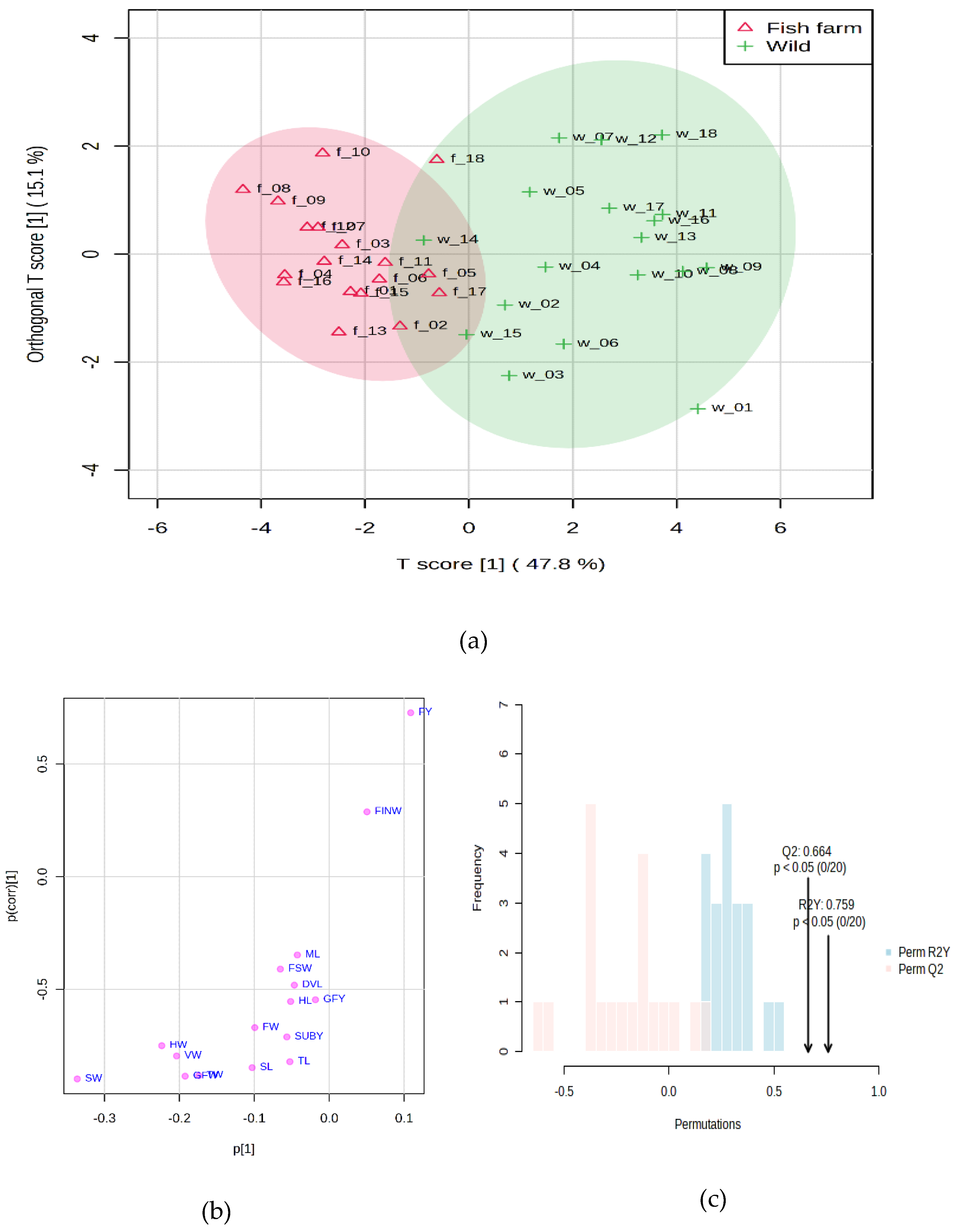
Figure 2a. The OPLS-DA score chart is displayed to visualize the separation between two groups based on entities. The T-score (47.8%) represents the variation in the data that is explained by the predictive component of the OPLS-DA model (related to clustering). In this case, the first component of the model explains 47.8% of the variation between wild and farmed fish based on the characteristics measured. The orthogonal T-score (15.1%) represents the variation in the data that is orthogonal (unrelated) to the clustering. This means that the first component also catches some variation that is unrelated to the difference between wild and farmed fish. It is often considered unexplained noise or variation. In this case, the first component captures 15.1% of this orthogonal variation.

The distribution of data points along the axis of the first component on the scorecard indicated the degree of separation between the groups. If the dots are well spaced along this axis, it means that the features are effective in distinguishing between wild fish and farmed fish. Since there are breeding conditions, there is some degree of similarity or shared variation between the two groups of breeding system (wild and fish farms).

Figure 2b shows the values that indicate the importance of each variable in the model for the first component (score) of the OPLS-DA analysis. The variable p [1] represents the contribution or magnitude of the covariance load of the variable concerning the scores of the model components. In simpler terms, it quantifies how much the variable contributes to the separation between the two fish farming groups based on their characteristics, such as SW (-0.33), HW (-0.22), VW (-0.20), and GFW (-0.19). The variable p(corr) [1] represents the effect and reliability of the variable’s correlation load for the model components’ scores. It indicates the strength with which the variation of the variable correlates with the separation between the groups, such as SW (-0.89), GFW (-0.88), TW (-0.88), SL (-0.84), TL (-0.82), VW (-0.79), HW (-0.75).

The results of the permutation analysis Figure 2c suggest that their OPLS-DA model has a statistically significant ability to predict differences between wild and farmed fish groups based on the measured characteristics. The observed value of Q² is 0.664. This value represents the actual predictive capability of the model in the original dataset. An R²Y value of 0.759 means that the model accounts for 75.9% of the variance in the response variable (clustering) using the features included in the analysis. The observed values of Q² and R²Y are higher than would be expected by chance, as indicated by the low p-values and the fact that neither permutation produced equal or more extreme results. This means that it is unlikely that the observed values of Q² and R²Y occurred just by chance. This provides confidence in the reliability of the model’s predictive capacity and the explanatory power of the included variables.

Table 3 shows the input variables used in the construction of an OPLS-DA model, along with their corresponding mean, standard deviation, maximum, and minimum values. In addition, the table includes the Variable Importance in Projection (VIP) values for each variable in the model. VIP values represent the importance of each variable in the projection and indicate its contribution to the classification or separation of the data. For the first component (VIP1), the SW variable (skeletal weight) has greater importance (VIP) in the discrimination between fish farming groups in Component 1 (V1) compared to Component 2 (V2). This suggests that the SW contributes more to the separation between the groups along the first component.

The weight of gutted fish (GFW) is of great importance in both components, suggesting that it contributes significantly to the separation between groups along both dimensions. Total weight (TW) is important in both components, indicating their substantial role in distinguishing between groups. Standard length (SL) is more important in Component 1 compared to Component 2, implying that it contributes more to the separation between groups along the first component. Overall length (TL) is important in both components, but it is more important in Component 1 compared to Component 2.

Viscera weight (VW) is more important in Component 1 compared to Component 2. Head weight (HW) is important in both components, indicating its contribution to the separation between groups along both dimensions. Fillet yield (AF) is most important in Component 1, suggesting its importance in distinguishing between groups along the first component. By-product yield (SUBY) is more important in Component 1 compared to Component 2.

3.3. Exploring the Multivariate ROC Curve Using the Random Forest Algorithm

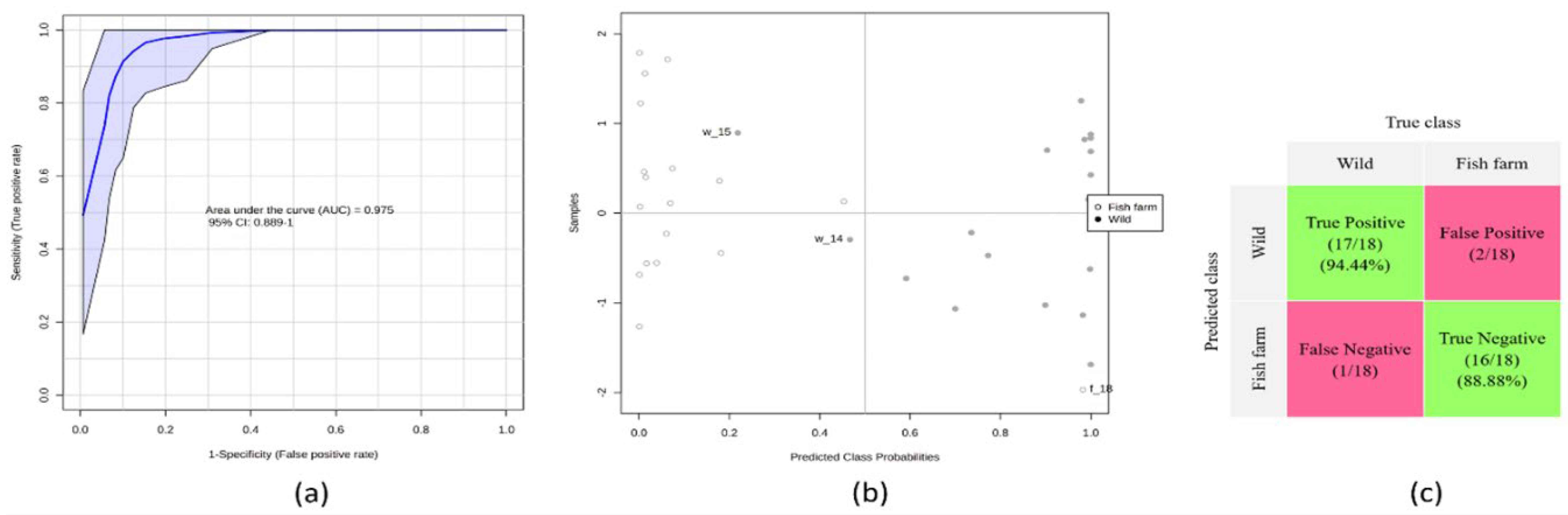
The ROC curve graph Figure 3a for the four-variable fish model shows promising results with average performance over the course of MCCV’s career. The area under the curve (AUC) value of 0.975 indicates a relatively high discriminative capacity of the model to distinguish between breeding systems (wild and fish farms).

The graph of class probabilities predicted for all samples using a single model yields insightful results, Figure 3b. This suggests that samples with predicted class probabilities below 0.5 are classified as one class, while those above 0.5 are classified as the other class. The balanced subsampling approach ensures equal representation of both classes, resulting in a classification boundary that aligns with the center. The false positives, indicated as 2 of 18 and 1 of 18, represent the number of samples that were incorrectly classified as the positive class while belonging to the negative class.

The confounding matrix provides valuable information about the performance of a Figure 3c classification model, especially in terms of sensitivity and specificity. In this case, the confounding matrix reveals that sensitivity and specificity are represented in the regions highlighted in green. Sensitivity, which measures the proportion of true positives correctly identified by the model, is determined at 94.44%. This indicates that the model successfully captures 94.44% of actual positive cases. On the other hand, specificity, which measures the proportion of true negatives correctly classified by the model, is at 88.88%.

The values generated for the area under the curve (AUC) (0.975) along with the 95% confidence intervals (CI) (0.889-1.000) are given within the graph and the accuracy is 90.80%. (b) Predicted class probabilities for each group, allowing the display of misclassified samples (fish farms are shown as white dots; wildcards are shown as black dots). Since a balanced subsampling approach is used for model training, the classification boundary is always in the center (x = 0.5, the dotted line). (c) Confusion matrix showing the number of true positives (17/18), true negatives (16/18), false positives (2/18), and false negatives (1/18). Sensitivity and specificity are found in the regions highlighted in purple, being 94.44% and 88.88% respectively.

The result provided in Table 4 presents the most important features of the selected model ranked in order of importance, along with descriptive statistics for four fish variables. The model used Random Forest and achieved an accuracy rate of 90.80%. The table indicates that the GFW variable occupies the highest range with a frequency of 1.00 and an importance value of 11.78. This implies that “GFW” plays a crucial role in the model’s predictions. It is followed by the variables “TW”, SL and SW with a frequency range of 0.94, 0.88 and 0.72 respectively and an importance value greater than 8, which indicates their significance in the model as well.

4. Discussion

According to the results, the fish farm system had a longer overall length than the wild rearing system with no difference in the three localities, while sex was surpassed by males. These results differ from the studies conducted [21] on the species Snook (Eleginops maclovinus), where there are differences in morphometry between individuals from different localities of Ecuador.

According to the study conducted by Soria et al. [6] for two species of old birds evaluated (Cichlidae), they expressed significant differences in fin length and cephalic region, from which the position of the mouth was statistically differentiated, which differs from our results, because it did not, they presented a significant difference in the length of the snout for any of the factors under study.

Regarding the size and shape of the species considering the areas evaluated, in the morphometric study of Guanchiche (Hoplias spp.) carried out by [22] showed that there are significant morphological differences between species, in geographically isolated populations of Hoplias spp. (different rivers) and between populations in different habitat types (rivers vs. dams). Although statistically significant, the morphological differences between males and females were very small, and it was generally not possible to distinguish between sexes based on body shape using geometric morphometry.

An acceptable yield of fillets according to [23] it should be between 30.0 and 35.0%. Species with a shorter head and longer trunk estimate that body dimensions are more appropriate for economic valuation because they have better use of their meat during primary processing and filleting.

According to [24] the yield values reported in our study are within the ranges of cichlids (Cichlidae) whose value ranges between 33.0-34.0%. Likewise, [5] they established that the commercially usable proportion based on the yield of the fillet and its by-products of the native Old Blue species was 94.65 and 33.92%, respectively, evaluating fish with an average total weight of 239.36 g. The pronounced size discrepancies observed between farmed and wild specimens could be attributed to several interrelated factors. Aquaculture environments typically provide controlled environments with consistent nutrition, reduced predation risks, and optimized conditions for growth. In contrast, wild habitats are characterized by varying food availability, competition, and predation pressures. The observed larger size of farmed specimens may be the result of improved nutritional provisioning and reduced stressors, facilitating accelerated growth rates. In addition, genetic selection in fish farms can favor traits conducive to rapid growth, contributing to the observed morphometric differences.

The significant differences observed in weight and yields across anatomical parts between wild and farmed specimens underscore the effectiveness of aquaculture in promoting growth acceleration and maximizing economic returns. Of note is the significant difference in yields of specific anatomical parts, such as the head and skeleton, where farmed specimens demonstrated substantially higher percentages. Skin-on fillet, a crucial economic component, also showed a notable increase in yield percentage for farmed specimens, indicating greater marketable yield potential in aquaculture environments.

The morphometric differences observed between localities can be attributed to different ecological conditions and habitat characteristics. The “Buena Fe” locality, characterized by its favorable climatic and soil conditions, exhibits a significantly longer total length compared to El Empalme and Mocache. This could be related to the availability of abundant resources, suitable for growth and development. Conversely, El Empalme and Mocache, with distinct climatic and topographic characteristics, can present challenges such as temperature fluctuations or limited food resources, affecting the overall size and proportions of the species. In addition, genetic variations between populations from different localities could contribute to the observed morphometric diversity.

Substantial differences in morphometric traits between males and females of A. rivulatus could be attributed to sexual dimorphism, a common phenomenon in many fish species. For example, the longer overall length and standard length observed in males may be associated with their reproductive strategy, where larger individuals are favored for mate selection or territorial defense. In addition, differences in dorsoventral length and head length could be related to secondary sexual characteristics, such as fin size and head morphology, which are often sexually dimorphic in fish. The length of the snout, which exhibits less disparity, may suggest a more conserved trait in all sexes, possibly indicating a shared functional role regardless of reproductive roles.

The successful implementation of OPLS-DA and Random Forest highlights their potential in fish classification tasks. Not only does OPLS-DA provide accurate classification, but it also offers insight into the latent structures that drive separation between fish classes. This application of OPLS-DA to fish classification in the context of reproductive variability contributes to expanding the repertoire of this technique beyond its traditional use in metabolomics and agriculture [25,26]. This information can contribute to a better understanding of the impact of rearing conditions on fish morphometry.

The ability of Random Forest’s algorithm to handle complex interactions between variables is particularly relevant in this study, as rearing conditions can introduce intricate variations in fish characteristics. The ensemble nature of Random Forest helps mitigate the influence of outliers and noise, improving the reliability of ranking results [27]. The use of the Random Forest algorithm for fish classification in the study aligns with previous applications in ecological contexts [28] and biological [29]. However, the novelty here lies in its application to the specific scenario of fish classification considering reproductive variability. The ensemble nature of the Random Forest allows it to capture nonlinear relationships and interactions between variables, which is particularly relevant when it comes to the nuanced effects of breeding conditions on fish characteristics such as gutted fish weight, total weight, standard length, and skeleton weight.

The novelty of the findings of this study arises from the integration of reproductive variability, the consideration of weight and height variables, and the application of machine learning techniques such as OPLS-DA and Random Forest for the classification of fish in Ecuador. These findings expand the current understanding of fish species identification and contribute to the advancement of both fisheries’ science and aquaculture management practices, ultimately encouraging more sustainable and ecologically informed approaches.

The findings have significant scientific relevance in the context of aquaculture practices and conservation efforts. Understanding the morphometric variations of Old Blue natives within different breeding systems is crucial to optimizing aquaculture practices to improve yield and economic sustainability. In addition, this research contributes to a broader understanding of the adaptability and plasticity of species in response to different environmental conditions. The observed differences provide insight into the potential consequences of introducing farm-reared individuals into natural habitats, with implications for ecological interactions and conservation strategies. This study contributes valuable data to the scientific discourse on the intersection of aquaculture, ecology, and species conservation, encouraging informed decision-making for sustainable resource management.

The results contribute to the understanding of the intraspecific variability of A. rivulatus in the Quevedo region. By identifying morphometric differences between localities, this study informs resource managers and conservationists about the potential impact of local environmental conditions on the species. This knowledge is crucial for designing specific conservation strategies and habitat management plans. In addition, the observed variations may have implications for the adaptability and resilience of the species to environmental changes, which is pertinent in the context of ongoing global environmental changes and habitat alterations. This study, therefore, improves our knowledge of the ecological dynamics of A. rivulatus and provides a basis for more nuanced and site-specific conservation efforts.

5. Conclusions

The morphometric study applied to the Old Blue examined the size and shape of native fish using measurable traits, such as standard length, total length, yields, among other measures. To classify the taxa and the level of species, the relationships obtained between these measures were of greater significance in the specimens reared in male fish farms, with the locality of El Empalme being the most representative. It was also observed that their fillet yields differ in the rearing systems. It represents an alternative for small and medium-sized fish farmers to breed the Old Blue in captivity due to consumer demand for its delicate meat and excellent animal protein.

References

- Motlagh, H.A.; Sarkheil, M.; Safari, O.; Paolucci, M. Supplementation of dietary apple cider vinegar as an organic acidifier on the growth performance, digestive enzymes and mucosal immunity of green terror (Andinoacara rivulatus). Aquac. Res. 2019, 51, 197–205. [CrossRef]
- Serdiati, N.; Yonarta, D.; Pratama, FS.; Faqih, AR.; Valen, F.S.; Tamam, MB.; Hasan, V. Andinoacara rivulatus (Perciformes: Cichlidae), an introduced exotic fish in the upstream of Brantas River, Indonesia. Aquac. Aquar. Conserv. Legis. 2020, 13, 137-141.
- Franco, M.; Arce, E. Aggressive interactions and consistency of dominance hierarchies of the native and nonnative cichlid fishes of the Balsas basin. Aggress. Behav. 2021, 48, 103–110. [CrossRef]
- Wijkmark, N.; Kullander, SO.; Barriga Salazar, RE. Andinoacara blombergi, a new species from the río Esmeraldas basin in Ecuador and a review of A. rivulatus (Teleostei: Cichlidae). Ichthyol. Explor. Freshw. 2012,23, 117.
- González, M.; Rodríguez, J.; López, M.; Vergara, G.; García, A. Estimación del rendimiento y valor nutricional de la vieja azul (Andinoacara rivulatus). Rev. De Investig. Talentos 2016, 3, 36-42.
- Soria-Barreto, M.; Rodiles-Hernández, R.; González-Díaz, AA. Morfometría de las especies de Vieja (Cichlidae) en ríos de la cuenca del Usumacinta, Chiapas, México. Rev. Mex. De biodiversidad 2011, 82, 569-579.
- Moshayedi, F.; Eagderi, S.; Rabbaniha, M. Allometric growth pattern and morphological changes of green terror Andinoacara rivulatus (Günther, 1860) (Cichlidae) during early development: Comparison of geometric morphometric and traditional methods. Iran. J. Fish. Sci. 2017, 16, 222-237.
- Prazdnikov, D.V. Influence of Triiodothyronine (T3) on the Reproduction and Development of the Green Terror Andinoacara rivulatus (Cichlidae). J. Ichthyol. 2018, 58, 953–958. [CrossRef]
- Caez, J.; Gonzalez, A.; González, M.A.; Angón, E.; Rodriguez, J.M.; Peña, F.; Barba, C.; Garcia, A. Application of multifactorial discriminant analysis in the morphostructural differentiation of wild and cultured populations of Vieja Azul (Andinoacararivulatus). Turk. J. Zoöl. 2019, 43, 516–530. [CrossRef]
- Gonzalez, A.; Angón, E.; González, M.; Rodriguez, J.; Barba, C.; García, A. Effect of rearing system and sex on the composition and fatty acid profile of Andinoacara rivulatus meat from Ecuador. Rev. de la Fac. de Cienc. Agrar. UNCuyo 2021, 53, 232–242. [CrossRef]
- De la Cruz-Torres, J.; González-Acosta, AF.; Martínez-Pérez, JA. Descripción y comparación de la línea lateral de tres especies de rayas eléctricas del género Narcine (Torpediniformes: Narcinidae). Rev. De Biol. Tropical 2018, 66, 586-592.
- Hubbs, C. L.; Lagler, K. F.; Smith, GR. Fishes of the Great Lakes region, revised edition (p. 332). Ann Arbor: University of Michigan Press. (2004).
- Chong, J.; Wishart, D.S.; Xia, J. Using MetaboAnalyst 4.0 for Comprehensive and Integrative Metabolomics Data Analysis. Curr. Protoc. Bioinform. 2019, 68, e86, . [CrossRef]
- Di Rienzo, J. A.; Casanoves, F., Balzarini, M. G., González, L., Tablada, M., Robledo, Y. C. InfoStat versión 2015. Grupo InfoStat, FCA, Universidad Nacional de Córdoba, Argentina. URL http://www. infostat. com. ar, 2015. 8, 195-199.
- Szymańska, E.; Saccenti, E.; Smilde, A.K.; Westerhuis, J.A. Double-check: validation of diagnostic statistics for PLS-DA models in metabolomics studies. Metabolomics 2011, 8, 3–16. [CrossRef]
- Olivares, B.O.; Vega, A.; Calderón, M.A.R.; Rey, J.C.; Lobo, D.; Gómez, J.A.; Landa, B.B. Identification of Soil Properties Associated with the Incidence of Banana Wilt Using Supervised Methods. Plants 2022, 11, 2070. [CrossRef]
- Bylesjö, M.; Rantalainen, M.; Cloarec, O.; Nicholson, J.K.; Holmes, E.; Trygg, J. OPLS discriminant analysis: combining the strengths of PLS-DA and SIMCA classification. J. Chemom. 2006, 20, 341–351. [CrossRef]
- Triba, M.N.; Le Moyec, L.; Amathieu, R.; Goossens, C.; Bouchemal, N.; Nahon, P.; Rutledge, D.N.; Savarin, P. PLS/OPLS models in metabolomics: the impact of permutation of dataset rows on the K-fold cross-validation quality parameters. Mol. Biosyst. 2014, 11, 13–19. [CrossRef]
- Breiman, L.; Last, M.; Rice, J. Random Forests: Finding Quasars. Stat. Chall. Astron. 2006, 45, 243–254. [CrossRef]
- Xu, Q.-S.; Liang, Y.-Z. Monte Carlo cross validation. Chemom. Intell. Lab. Syst. 2001, 56, 1–11. [CrossRef]
- Xia, J.; Wishart, D.S. Using MetaboAnalyst 3.0 for Comprehensive Metabolomics Data Analysis. Curr. Protoc. Bioinform. 2016, 55, 14.10.1–14.10.91. [CrossRef]
- Gacitúa, S.; Oyarzún, C.; Veas, R. Análisis multivariado de la morfometría y merística del robalo Eleginops maclovinus (Cuvier, 1830). Rev. De Biol. Mar. Y oceanografía 2008, 43, 491-500.
- Granda, J. C.; Montero, CS. Aplicación de Morfometría Geométrica para la Comparación de Distintas Poblaciones de Guanchiche (Hoplias spp) en Ecosistemas Lénticos y Lóticos del Ecuador (Bachelor’s thesis). 2015.
- Eslava, E. Estimation of yield and nutritional value of Bobo Mullet (Joturus pichardi Poey, 1860) (Pisces: Mugilidae). Rev. MVZ Córdoba 2009, 14, 1576-1586.
- Sulieman, HA.; James, GK. A comparative studies on the chemical and physical attributes of wild farmed Nile tilapia (Oreochromis niloticus). Online J. Anim. Feed. Res. 2011, 1, 407-411.
- Olivares, B.O.; Rey, J.C.; Perichi, G.; Lobo, D. Relationship of Microbial Activity with Soil Properties in Banana Plantations in Venezuela. Sustainability 2022, 14, 13531. [CrossRef]
- Olivares, B.O.; Vega, A.; Calderón, M.A.R.; Montenegro-Gracia, E.; Araya-Almán, M.; Marys, E. Prediction of Banana Production Using Epidemiological Parameters of Black Sigatoka: An Application with Random Forest. Sustainability 2022, 14, 14123. [CrossRef]
- Campos, BO. Banana Production in Venezuela: Novel Solutions to Productivity and Plant Health. Springer Nature, Switzerland. 2023.
- Rodríguez-Yzquierdo, G.; Olivares, BO.; Silva-Escobar, O.; González-Ulloa, A.; Soto-Suarez, M.; Betancourt-Vásquez, M. Mapping of the susceptibility of Colombian Musaceae lands to a deadly disease: Fusarium oxysporum f. sp. cubense Tropical Race 4. Horticulturae 2023, 9, 757.