
Submitted:
05 September 2025
Posted:
08 September 2025
You are already at the latest version
Abstract
During the last two decades relevant progress has been achieved in silicon photomultiplier (SiPM) technology, so that in an increasing number of radiation detection applications they are proposed as a viable alternative to traditional photomultiplier tubes (PMT). Applications where the light from tiny scintillating crystals is detected by a single SiPM raise the question of the possible non-linearity of the response due to saturation of the number of microcells involved. In other cases where larger scintillators subtend arrays of SiPMs the same question could hold. This work tries to disentangle such a question with a realistic numerical approach and a few tests, showing that possible saturation effects depend on the interplay between the features of the scintillator and of the SiPM (array). The quantitative results of this analysis can likely be used to better plan future radiation detection systems and to highlight their linearity boundaries.
Keywords:
silicon photomultiplier
; scintillator
; non-linearity
1. Introduction
The detection of gamma rays is one of the most widespread applications in radiation physics worldwide. Whenever high spectroscopic precision is required, in order to identify the emitting radioisotopes, the gold standard of detectors is the germanium semiconductor [1]. In most other cases much less expensive and more practical detectors based on scintillators are exploited. A scintillator detector is based on special organic or inorganic materials exhibiting the notable feature of producing tiny flashes of light when hit by radiation. We will not go into details of how such a light is produced at molecular level, but we just remind here that the produced visible photons are emitted isotropically according to an exponential time distribution with a decay constant µ characteristic of each material. Organic scintillators are typically faster, with µ values even down to 1-2 ns, whereas inorganic crystals span a wide range from tens of nanoseconds even up to milliseconds [2,3].
Throughout several decades the light readout of scintillators has mainly been performed by means of photomultiplier tubes (PMT), until more recently a new kind of solid state photodetector has come onto the playground, namely the silicon photomultiplier (SiPM). Such a device, suggested many years ago but only recently industrially produced because of relevant technological advances, operates according to a quasi-digital scheme. Indeed, it consists of an array of semiconductor microcells kept in a quiescent state slightly above the breakdown voltage. When a visible photon interacts with one such microcell it triggers a discharge, limited by a built-in quenching resistor, that gives rise to a signal consisting of the electrical charge stored in the microcell itself. Being all microcells identical, each one produces the same signal when hit by a visible photon and then a light pulse consisting of n photons should produce a signal n times as large as the single photon does.
Of course this ideal scheme has several limitations in real sensors:
- Only a fraction of the photons hitting the SiPM produces signals, because of its photon detection efficiency (PDE) that is far from 100%;
- When two or more photons interact with the same microcell the produced signal is the same (this is the so called problem of the multiple hit);
- Each microcell has a recharging dead time, i.e., a short time interval after being triggered, during which it is inactive because its voltage is being restored to the operating value;
- As the microcells are kept above breakdown, every now and then they can spontaneously discharge for thermal reason, giving rise to an overall poissonian dark noise mainly consisting of single microcell signals plus rarer double, triple and higher order spurious coincidences.
However, the main limitation of SiPMs is their maximum size, that for the currently available devices is 6 mm × 6 mm. Such a small size can also be seen as an advantage, should one be interested to set up a miniature gamma ray detector. Due to the decreasing cost of these photosensors, the size limitation is currently being overcome by arranging arrays of SiPMs for the readout of larger scintillators. Details on the features and operation of SiPMs can be found in [4,5,6,7] and in the copious list of references therein.
One of the questions arising from the above mentioned operational limitations is the linearity of the response, in particular when detecting gamma rays of the order of 1-2 MeV [8,9,10,11]. In this work we examine the behavior of two different models of SiPM, when coupled to five popular scintillators, as a function of the energy deposited by gamma rays. In Section 2 we describe the algorithm developed to evaluate the behavior of a SiPM illuminated by scintillation light, and in Section 3 we show the results obtained with the several examined combinations of scintillator + SiPM along with the experimental results obtained in two particular real cases. Finally, in Section 4 we discuss the relevant take-home messages arising from our results.
2. Materials and Methods
2.1. Detecting Gamma Rays
The interaction of gamma rays with matter occurs according to three main processes:
- Photoelectric effect, dominating at low energy, when the gamma disappears transferring all of its energy to an electron;
- Compton scattering, dominating at intermediate energy, with the gamma scattering off an electron and imparting it some kinetic energy;
- e+e- pair creation close to a nucleus, exploiting 1.022 MeV of the incoming gamma thus being the dominating effect at very high energy.
For the low to medium energy range considered here, namely up to ≈ 2 MeV, only photoelectric effect and Compton scattering are relevant. The energetic electron thus produced interacts with other electrons and gives rise to a so called shower, i.e., a cloud of energetic electrons whose total kinetic energy is equal to the energy released by the initial gamma interaction. The scintillation light in scintillators is produced by the interaction of these energetic electrons with "color centers", i.e., typically dopants in the material capable to reach an excited level by collision which deexcites by emitting visible light. The number of visible photons produced in each gamma interaction is generally proportional to the energy deposited by the gamma ray into the material. The detection and energy measurement of the gamma rays is done by measuring the amount of scintillation light produced by means of some photodetector which converts light into an electric signal. Due to the very small amount of light produced a physical amplification is quite often required, and the task is accomplished by using a photomultiplier device.
Different scintillators have different linearity between deposited energy and scintillation light, especially at high deposited energy where some saturation of the light yield could be expected. Saturation can also be expected due to the employed photosensor, especially in the case of photoelectric interaction when the full gamma energy is transferred to the material. Starting from our previous experience with detectors based on scintillators and SiPMs [12,13,14,15], we examined five popular scintillation materials, whose main features relevant for this study are listed in Table 1 [16], and their response when coupled to two models of 6 mm × 6 mm SiPM [17,18] whose features are listed in Table 2.
2.2. Collecting the Scintillation Light
The number of scintillation photons collected on the photosensor depend on the geometric features of the detector and, more important, on the type and quality of the outer surface of the scintillator. Indeed, a bare scintillator would lose most of the light through its outer faces, and basically collecting only those photons traveling straight from the emission point to the photosensor. This is why scintillators are generally coated with a highly reflective layer (paint, resin, ...) to maximize the light collection efficiency allowing photons to be collected also after several internal reflections. The reflector is not specular but white so that, contrary to the case of geometrical reflection, the light path inside the scintillator is quickly randomized. This way any possible variation of the light collection efficiency with its emission position inside the scintillator is minimized. The typical reflectivity values of the employed reflector materials range from 0.9 to 0.96.
Two detector geometries have been examined, representative of two major possible approaches to the spectroscopic detection of gamma rays with scintillators and SiPMs. The first one concerns applications as miniature detectors and dosimeters, whereas the second has crystal size and shape typical of several existing commercial products:
The results and considerations that we are going to describe in the following can be easily rescaled to similar geometrical configurations with larger or smaller scintillators and different number of SiPMs.
Due to the compact size of both geometries with respect to the (re)absorption length of several tens of centimeters for all of the scintillators under consideration, in this study we decided to neglect the possible self-absorption of scintillation photons in the scintillator material. The light collection efficiency, i.e., the fraction of photons reaching the SiPM, was first estimated by means of a simple naive approach:
- No real geometry is considered for the system and no light propagation is implemented;
- A scintillation photon produced somewhere inside the crystal reaches a point on the inner surface;
- We assume it can hit the SiPM with a probability ε roughly equal to the ratio between the area of the SiPM and the total area of the crystal;
- Otherwise it can be reflected or absorbed with probability r and (1−r) respectively, being r the reflectivity of the inner surface.
- We denote with P1 = ε the probability that the photon is collected directly on the first step, with P2 the probability that the photon is collected after one reflection (i.e., at the second step), and so on;
- After each step the probability of the photon to be still available is (1−ε)r (i.e., not collected and reflected), whereas the probability to be collected at the following step is still ε.
- The sum of all the probabilities of collection in any number of steps, thus regardless of the number of reflections, represents the light collection efficiency (Eq.1).
This calculation was done for several values of the reflectivity ranging from 0.9 to 1, with the elementary collection probabilities ε = 0.06 and ε = 0.084 given by the area ratios for the cases of Figure 1a,b.
In order to support or disprove these results we performed a set of more sophisticated Monte Carlo simulation runs by means of Geant4 [24]. The inner surfaces of the scintillator were assumed to produce diffuse Lambertian reflection [25], each run with a different value of the reflectivity. Inside the crystal we generated randomly 105 scintillation photons per run, following each one throughout its path and reflections until being absorbed in a wall or reaching the photosensor. The two geometries of Figure 1 were implemented and eleven runs per configuration were performed, with the reflectivity of the walls ranging from 0.9 to 1 in steps of 0.1. The runs with reflectivity equal to one showed that the average time for the detection is 0.62 ns and 1.6 ns respectively, which assuming a refractive index around 1.9 correspond to average path lengths of the order of 10 and 25 cm. In case of reflectivity equal to 0.95 these values roughly halve to about 5.5 and 13 cm, much smaller than the attenuation length values in the considered crystals, thus justifying the choice of neglecting the self-absorption.
The resulting values of the light collection efficiency for the two approaches and for the two detector geometries are plotted in Figure 2. Surprisingly, the differences between the simple and the Monte Carlo approaches are quite small thus suggesting that the simple formula of Eq.1 can realistically be used for future evaluations of similar configurations. Curiously, we also found empirically that if one increases the ε value for both geometries to ε+ = ε × 1.067, thus obtaining ε+ = 0.064 and ε+ = 0.090, the two approaches would become equal well below the percent level, and this holds for both geometrical configurations. This aspect could perhaps be worth future additional investigation. The ratio between simple and Geant4 values is plotted in Figure 3 for the cube and the cylinder geometries. Also plotted are the same ratios for the cases of empirically increased ε values. The data of Figure 2 and Figure 3 are also listed in Table A1 and Table A2 of Appendix A. However, for all of the following calculations we decided to use the light collection efficiency values of P ≈ 0.56 and P ≈ 0.65 resulting from Eq.1 for cube and cylinder geometries respectively, choosing a reflectivity value of r ≈ 0.95 and the above mentioned elementary collection probabilities ε = 0.06 and ε = 0.084.
2.3. Detecting the Collected Light
The physical quantities to be considered for the detection with SiPMs are the light yield of the crystal, the light decay time, the emission spectrum, the collection efficiency of the chosen detector geometry, the SiPM's PDE, its number of microcells, the microcell recharge time (i.e., dead time). If we want to calculate the expected response of the photosensor we have to take into account all these quantities at the same time. We used the values listed on Table 1 and Table 2, and in order to show the behavior of the decay time in real operation we plotted in Figure 4 a signal waveform acquired from a CsI(Tl) scintillator coupled to a SensL SiPM in the configuration of Figure 1a with a digital scope. An exponential fit to the waveform produces a decay constant µ = 0.96 µs as expected.
As for the PDE, we multiplied the PDE(λ) function of each SiPM [17,18] by the light emission spectra of the five scintillators [19,20,21,22,23] (Figure 5) normalized to unit area. The integral of such a convolution represents the effective PDE of each SiPM when detecting the light emitted by each scintillator. The resulting values are reported in Figure 6.
There are two different mechanisms possibly leading to loss of linearity in a SiPM: (i) signal saturation due to multiple photons interacting with the same microcell but being detected as one; (ii) loss of photons due to microcells hit during their recharge dead time because of a previous hit. The number of microcells actually fired by a bunch of photons can be smaller than the number of electron avalanches generated in the SiPM, because two or more avalanches generated in the same microcell produce the same signal and thus are seen as one. The most probable number of microcells f(q) actually triggered (i.e., when a photoelectron is produced capable of producing an avalanche) by a bunch of q photons impinging randomly on a SiPM with m microcells and PDE equal to p can be evaluated based on the binomial distribution.
- is the probability for a single microcell to be triggered by one impinging photon;
- is the probability that a single microcell is not triggered by one impinging photon;
- is the probability that a single microcell is not triggered by q impinging photons;
- is the probability that a single microcell is triggered by at least one of the q impinging photons.
As there are m microcells the expected number of triggered ones is
By exploiting the notable limit shown below
one obtains the much simpler approximate formula
The effect of the possible loss due to dead time of recharging microcells requires to consider the time development of the light pulse. Therefore we developed a simple algorithm that considers the production of photons exponentially decreasing in time with the decay constant of the scintillator, using time slots of 5 ns. In each time slot the number of triggered microcells is calculated by means of Eq.4, using a variable number of available microcells m calculated on the basis of the number of previously triggered ones and of their recharge time which makes them temporarily unavailable. The algorithm follows the light pulses during few microseconds, that is much longer than the slowest decay constant of the considered scintillators, and calculates the sum of all the numbers of triggered microcells that is proportional to the integral of the output signal.
3. Results
The combination of the light decay constant of the scintillator with the microcell recharge time of the SiPM produces an initial decrease of the number of available microcells that could or could not influence significantly the linearity of the SiPM response, depending on the deposited energy, on the scintillator type, and on the total number of microcells. In Figure 7a we show as an example the number of triggered and of available microcells as a function of time, for the case of 2 MeV deposited in a 1 cm × 1 cm × 1 cm CsI(Tl) crystal read by the SensL SiPM. Also shown is the ideal number of microcells that would be triggered if no recharge dead time were present. In Figure 7b we plotted the ratio between the number of fired microcells to the ideal one as a function of time. It can be seen that in this case the initial decrease in the number of available microcells does not influence the overall linear response, as there is no appreciable difference between the ideal and the effective total numbers of triggered cells. Figure 8 shows the corresponding plots for the case of the same scintillator coupled to the Hamamatsu SiPM. Even in this case the response is basically linear, even though the non-linearity is slightly larger to due to the smaller number of microcells. Figure 9, Figure 10, Figure 11, Figure 12, Figure 13, Figure 14, Figure 15 and Figure 16 show the similar plots for all the other combinations of scintillator and SiPM listed in Table 1 and Table 2 respectively. It can be immediately observed that LaBr3(Ce) and CeBr3 give rise to an enormous non-linearity due to the large amount of scintillation photons reaching the SiPM in a very short time interval, thus totally blinding it for a while and losing a considerable fraction of the light signal. In Figure 17 we summarize the results from Figure 7, Figure 8, Figure 9, Figure 10, Figure 11, Figure 12, Figure 13, Figure 14, Figure 15 and Figure 16 by integrating the plots over time: (a) the total number of ideal hits and of actually triggered microcells for all the examined configurations of scintillator and SiPM; (b) the expected non-linearity i.e., 1−(triggered/ideal).
As for the cylindrical configuration no SiPM blinding occurs, as expected due to the 16 times larger number of microcells, and as a consequence the non-linearity is much smaller in all configurations. We only show the time evolution plots for the worst case, which is the one related to the CeBr3 scintillator that has the highest light yield and the fastest decay time, in Figure 18 and Figure 19 respectively for the SensL and Hamamatsu SiPMs. Figure 20 summarizes the results for the cylindrical configurations. Then we also calculated the total number of triggered microcells as a function of the gamma energy deposited inside the scintillator for all the combinations of scintillator and SiPM listed in Table 1 and Table 2 respectively, for the two geometries of Figure 1. The resulting values are plotted in Figure 21 and Figure 22, and are also listed in Table A3, Table A4, Table A5 and Table A6 of Appendix B. The plot of Figure 21 shows that the CsI(Tl), BGO and NaI(Tl) cubic scintillators coupled with either SiPM are expected to be linear in the full investigated energy range. A relevant nonlinearity appears instead above ≈ 1500 keV (SensL) and ≈ 900 keV (Hamamatsu) for LaBr3(Ce) and CeBr3: this represents the onset of the SiPM blinding because of the much faster decay constant of both scintillators (30 and 20 ns). These features tend to concentrate a larger number of hits in fewer microcells in a much shorter time interval. Conversely, Figure 22 shows that in the cylindrical configuration read by 16 SiPMs the behavior is basically linear with all the scintillators and both SiPMs despite the small non-linearities visible in Figure 20b.
In Figure 23a and c we show two sets of spectra, taken with 1 cm × 1 cm × 1 cm CsI(Tl) crystals, read by a SensL and by a Hamamatsu SiPM respectively. Each spectrum is related to one of four gamma sources (226Ra, 22Na, 137Cs, 60Co). The data were available from previous experiments and unfortunately they were taken using different sets of sources with different activities, this is why each spectrum was normalized to its own integral. Figure 23b and d report the corresponding energy calibrations, Table 3 lists the energy values of the peaks used in the calibration for each source. The two highest energy peaks, from 226Ra, were not used for the calibration but just for a linearity cross check.
4. Discussion
The main indication from our results is that, when planning to set up a spectroscopic gamma-ray detector based on scintillator and SiPMs, careful consideration should be given both to the choice of components and to the energy range of interested. Indeed, there is a relevant interplay between the light yield of the scintillator, its decay time, the number of microcells featured by the SiPM, and the microcell recharge dead time. The SiPM, as a quasi-digital counter, has a finite number of microcells and this can give rise to a partial saturation of the output signal due to:
- Two or more photons interacting with the same microcell (multiple hit);
- A number of microcells temporarily inactive because they are recharging after being triggered.
The two effects take place massively with LaBr3 and CeBr3 scintillators, whose light emission produces a large number of photons in a very short time interval. This causes non-linearity when the deposited energy is small, but can totally blind the SiPM for a while in case of large deposited energy in the small scintillator cube (see Figure 9, Figure 10, Figure 11 and Figure 12, and 21). The effect is more pronounced in the SiPM with a smaller number of microcells (Hamamatsu). The time-integrated non-linearities shown in Figure 17 are the result of the above mentioned interplay. In the bigger cylindrical configuration there is a relevant advantage, i.e., the number of photons produced is shared among several SiPMs so that each one sees only a fraction of them. In such a case the non-linearities are strongly reduced, as can be seen in the worst-case plots of Figure 18, Figure 19 and Figure 22.
If one is interested in setting up a small scintillator with a single SiPM the best candidate seems to be CsI(Tl), either using a SensL or a Hamamatsu SiPM. Indeed CsI(Tl) represents the best trade-off between linearity, energy resolution (Table 4), and chemical properties:
- LaBr3(Ce) and CeBr3, hygroscopic thus requiring an expensive air-tight case, are strongly non-linear as they blind the SiPM;
- NaI(Tl) is rather equivalent to CsI(Tl) but it is hygroscopic;
- BGO has a poor light yield, therefore the SiPM light readout would be perfectly linear but providing a poor energy resolution.
- CsI(Tl) is reasonably inexpensive as compared to LaBr3(Ce), CeBr3 and NaI(Tl), and does not require any special air-tight case thus being easy to manipulate.
Despite some claim about the possible non-linearity of similar SiPMs when detecting gamma rays above 1 MeV or less when coupled to CsI(Tl) [10], our calculations show no indication of such an effect. Indeed, Figure 23 shows a slight loss of linearity above 1.7 MeV for both the SensL and the Hamamatsu SiPMs, but this is likely to be ascribed to a non-linearity of the crystal itself, as it was also suggested in [11].
We remark that the energy resolution values quoted in Table 4 do not consider corrections for the Fano factor, and they were simply calculated as Poisson uncertainty from the number of triggered microcells (inverse square root multiplied by 2.35). However, they provide realistic indications, in particular for LaBr3(Ce) and CeBr3.
As a further exercise we used our calculation method to investigate how the non-linearity evolves for bigger cubic geometries, only considering LaBr3(Ce) and CeBr3 scintillators because they are the only ones creating relevant non-linearity with SiPM readout. Therefore we evaluated the expected non-linearity at 2 MeV deposited energy for the two additional cubic configurations of Figure 24. In Table 5 we summarize the main features of these configurations along with the previously shown cubic and cylindrical ones for comparison, and in Figure 25 we compare the corresponding results which show a relevant linearity improvement and no SiPM blinding.
5. Conclusions
The results of our numerical analysis can likely be used when planning future radiation detection systems based on scintillators and SiPMs, as it somehow highlights their realistic linearity boundaries. The analysis also confirms the quite interesting properties of the CsI(Tl) scintillator, as it represents a good compromise between cost, performance, and ease of use, especially if planning to employ it in miniature detection systems like personal dosimeters. For higher level spectroscopic applications of scintillators the feasibility of larger cylindrical configurations, coupled to arrays of SiPMs, has been confirmed up to a few MeV. LaBr3(Ce) and CeBr3 are the best options in terms of timing and energy resolution, even though CsI(Tl) remains a notable candidate as well.
Supplementary Materials
The following supporting information can be downloaded at the website of this paper posted on Preprints.org. The following supporting files have been submitted along with this manuscript: time_evolution_cube.xlsx, time_evolution_cyl.xlsx
Author Contributions
Conceptualization, P.F., C.R.F., S.A. and G.E.P.; methodology, P.F., C.R.F., S.A. and G.E.P.; software, P.F. and S.A.; validation, P.F., C.R.F., S.A. and G.E.P.; formal analysis, P.F.; investigation, P.F. and S.A.; resources, P.F.; data curation, P.F., C.R.F., S.A. and G.E.P.; writing—original draft preparation, P.F.; writing—review and editing, P.F., C.R.F., S.A. and G.E.P.; visualization, P.F.; supervision, P.F.; project administration, P.F.; funding acquisition, P.F. All authors have read and agreed to the published version of the manuscript.
Funding
S. Amaducci was supported by PNRR SAMOTHRACE - codice ecs00000022 - cup I63C21000320006 - M4 - C2 - inv. 1.5 - avviso n. 3277 del 30-12-2021.
Data Availability Statement
The following supporting files have been submitted along with this manuscript: time_evolution_cube.xlsx, time_evolution_cyl.xlsx
Conflicts of Interest
The authors declare no conflicts of interest.
Appendix A

Table A1.
Cube configuration: light collection efficiency results from Geant4 simulation, from our simple model and from the simple model with increased ℇ value (these data are plotted on Figure 2a and Figure 3a).
| reflectivity | Geant4 | simple model | simple/Geant4 | ℇ+ model | ℇ+/Geant4 |
| 0.9 | 40.8% | 39.0% | 0.95 | 40.6% | 0.99 |
| 0.91 | 43.6% | 41.5% | 0.95 | 43.2% | 0.99 |
| 0.92 | 46.1% | 44.4% | 0.96 | 46.1% | 1.00 |
| 0.93 | 49.1% | 47.7% | 0.97 | 49.4% | 1.01 |
| 0.94 | 53.1% | 51.5% | 0.97 | 53.3% | 1.00 |
| 0.95 | 57.9% | 56.1% | 0.97 | 57.8% | 1.00 |
| 0.96 | 62.8% | 61.5% | 0.98 | 63.1% | 1.00 |
| 0.97 | 69.4% | 68.0% | 0.98 | 69.5% | 1.00 |
| 0.98 | 77.0% | 76.1% | 0.99 | 77.4% | 1.00 |
| 0.99 | 87.0% | 86.5% | 0.99 | 87.2% | 1.00 |
| 1 | 100.0% | 100.0% | 1.00 | 100.0% | 1.00 |
Table A2.
Cylinder configuration: light collection efficiency results from Geant4 simulation, from our simple model and from the simple model with increased ℇ value (these data are plotted on Figure 2b and Figure 3b).
| reflectivity | Geant4 | simple model | simple/Geant4 | ℇ+ model | ℇ+/Geant4 |
| 0.9 | 49.5% | 47.9% | 0.97 | 49.7% | 1.00 |
| 0.91 | 52.5% | 50.5% | 0.96 | 52.3% | 1.00 |
| 0.92 | 55.4% | 53.5% | 0.97 | 55.2% | 1.00 |
| 0.93 | 58.3% | 56.8% | 0.97 | 58.5% | 1.00 |
| 0.94 | 62.0% | 60.5% | 0.98 | 62.2% | 1.00 |
| 0.95 | 66.3% | 64.8% | 0.98 | 66.4% | 1.00 |
| 0.96 | 71.2% | 69.7% | 0.98 | 71.2% | 1.00 |
| 0.97 | 76.6% | 75.4% | 0.98 | 76.7% | 1.00 |
| 0.98 | 83.1% | 82.1% | 0.99 | 83.1% | 1.00 |
| 0.99 | 90.7% | 90.2% | 0.99 | 90.8% | 1.00 |
| 1 | 100.0% | 100.0% | 1.00 | 100.0% | 1.00 |
Appendix B
Table A3.
Number of triggered microcells as a function of deposited gamma energy for the cubic configuration of Figure 1a with the SensL SiPM (data plotted in Figure 21a).
| Edep [keV] | CsI(Tl) | LaBr3(Ce) | CeBr3 | BGO | NaI(Tl) |
| 100 | 907 | 1212 | 1327 | 162 | 882 |
| 200 | 1814 | 2417 | 2642 | 325 | 1763 |
| 300 | 2721 | 3615 | 3944 | 487 | 2644 |
| 400 | 3628 | 4805 | 5232 | 650 | 3525 |
| 500 | 4534 | 5988 | 6506 | 812 | 4405 |
| 600 | 5441 | 7162 | 7765 | 974 | 5284 |
| 700 | 6347 | 8326 | 9008 | 1137 | 6163 |
| 800 | 7254 | 9481 | 10233 | 1299 | 7042 |
| 900 | 8160 | 10624 | 11439 | 1461 | 7920 |
| 1000 | 9066 | 11755 | 12622 | 1623 | 8798 |
| 1100 | 9972 | 12873 | 13782 | 1786 | 9675 |
| 1200 | 10878 | 13975 | 14913 | 1948 | 10551 |
| 1300 | 11783 | 15059 | 16010 | 2110 | 11427 |
| 1400 | 12689 | 16121 | 17063 | 2272 | 12303 |
| 1500 | 13594 | 17153 | 18055 | 2435 | 13177 |
| 1600 | 14500 | 18145 | 18926 | 2597 | 14051 |
| 1700 | 15405 | 19064 | 19099 | 2759 | 14925 |
| 1800 | 16310 | 19637 | 19106 | 2921 | 15798 |
| 1900 | 17215 | 19674 | 19113 | 3083 | 16670 |
| 2000 | 18120 | 19710 | 19120 | 3246 | 17541 |
| 2100 | 19024 | 19747 | 19127 | 3408 | 18412 |
| 2200 | 19929 | 19783 | 19134 | 3570 | 19282 |
| 2300 | 20833 | 19820 | 19141 | 3732 | 20151 |
| 2400 | 21737 | 19856 | 19148 | 3894 | 21019 |
| 2500 | 22641 | 19893 | 19155 | 4056 | 21887 |
Table A4.
Number of triggered microcells as a function of deposited gamma energy for the cubic configuration of Figure 1a with the Hamamatsu SiPM (data plotted in Figure 21b).
| Edep [keV] | CsI(Tl) | LaBr3(Ce) | CeBr3 | BGO | NaI(Tl) |
| 100 | 1377 | 1638 | 1750 | 246 | 1209 |
| 200 | 2754 | 3259 | 3471 | 493 | 2417 |
| 300 | 4131 | 4861 | 5160 | 739 | 3624 |
| 400 | 5507 | 6442 | 6812 | 985 | 4830 |
| 500 | 6883 | 7998 | 8424 | 1232 | 6034 |
| 600 | 8259 | 9524 | 9986 | 1478 | 7238 |
| 700 | 9634 | 11013 | 11487 | 1724 | 8439 |
| 800 | 11009 | 12452 | 12902 | 1970 | 9640 |
| 900 | 12383 | 13811 | 14159 | 2216 | 10839 |
| 1000 | 13758 | 14901 | 14449 | 2462 | 12036 |
| 1100 | 15131 | 14973 | 14461 | 2708 | 13232 |
| 1200 | 16504 | 15032 | 14473 | 2954 | 14426 |
| 1300 | 17877 | 15090 | 14485 | 3200 | 15618 |
| 1400 | 19249 | 15148 | 14497 | 3446 | 16808 |
| 1500 | 20621 | 15207 | 14508 | 3692 | 17996 |
| 1600 | 21993 | 15265 | 14521 | 3938 | 19181 |
| 1700 | 23364 | 15323 | 14533 | 4184 | 20364 |
| 1800 | 24734 | 15381 | 14544 | 4429 | 21544 |
| 1900 | 26104 | 15440 | 14556 | 4675 | 22721 |
| 2000 | 27474 | 15497 | 14568 | 4921 | 23896 |
| 2100 | 28843 | 15556 | 14580 | 5166 | 25066 |
| 2200 | 30211 | 15614 | 14592 | 5412 | 26233 |
| 2300 | 31579 | 15673 | 14604 | 5657 | 27396 |
| 2400 | 32947 | 15731 | 14616 | 5903 | 28554 |
| 2500 | 34314 | 15789 | 14628 | 6148 | 29707 |
Table A5.
Number of triggered microcells as a function of deposited gamma energy for the cylindrical configuration of Figure 1b with the SensL SiPM (data plotted in Figure 22a).
| Edep [keV] | CsI(Tl) | LaBr3(Ce) | CeBr3 | BGO | NaI(Tl) |
| 100 | 907 | 1215 | 1332 | 162 | 882 |
| 200 | 1814 | 2430 | 2664 | 325 | 1764 |
| 300 | 2721 | 3644 | 3995 | 487 | 2646 |
| 400 | 3629 | 4858 | 5325 | 650 | 3528 |
| 500 | 4536 | 6071 | 6655 | 812 | 4410 |
| 600 | 5443 | 7284 | 7984 | 974 | 5292 |
| 700 | 6350 | 8496 | 9312 | 1137 | 6173 |
| 800 | 7257 | 9709 | 10639 | 1299 | 7055 |
| 900 | 8164 | 10920 | 11966 | 1462 | 7937 |
| 1000 | 9071 | 12132 | 13291 | 1624 | 8819 |
| 1100 | 9978 | 13342 | 14616 | 1786 | 9700 |
| 1200 | 10886 | 14553 | 15941 | 1949 | 10582 |
| 1300 | 11793 | 15763 | 17264 | 2111 | 11464 |
| 1400 | 12700 | 16973 | 18587 | 2274 | 12345 |
| 1500 | 13607 | 18182 | 19909 | 2436 | 13227 |
| 1600 | 14514 | 19391 | 21230 | 2598 | 14109 |
| 1700 | 15421 | 20599 | 22551 | 2761 | 14990 |
| 1800 | 16328 | 21807 | 23871 | 2923 | 15872 |
| 1900 | 17235 | 23014 | 25190 | 3085 | 16753 |
| 2000 | 18142 | 24222 | 26508 | 3248 | 17635 |
| 2100 | 19049 | 25428 | 27825 | 3410 | 18516 |
| 2200 | 19956 | 26634 | 29142 | 3573 | 19398 |
| 2300 | 20863 | 27840 | 30458 | 3735 | 20279 |
| 2400 | 21770 | 29046 | 31773 | 3897 | 21161 |
| 2500 | 22677 | 30250 | 33087 | 4060 | 22042 |
Table A6.
Number of triggered microcells as a function of deposited gamma energy for the cylindrical configuration of Figure 1b with the SensL SiPM (data plotted in Figure 22b).
| Edep [keV] | CsI(Tl) | LaBr3(Ce) | CeBr3 | BGO | NaI(Tl) |
| 100 | 1378 | 1646 | 1763 | 246 | 1210 |
| 200 | 2755 | 3291 | 3525 | 493 | 2419 |
| 300 | 4133 | 4935 | 5284 | 739 | 3629 |
| 400 | 5510 | 6578 | 7042 | 986 | 4838 |
| 500 | 6888 | 8220 | 8799 | 1232 | 6047 |
| 600 | 8265 | 9861 | 10553 | 1478 | 7256 |
| 700 | 9642 | 11500 | 12306 | 1725 | 8466 |
| 800 | 11020 | 13139 | 14057 | 1971 | 9675 |
| 900 | 12397 | 14777 | 15807 | 2218 | 10884 |
| 1000 | 13775 | 16414 | 17554 | 2464 | 12093 |
| 1100 | 15152 | 18050 | 19300 | 2710 | 13302 |
| 1200 | 16529 | 19685 | 21044 | 2957 | 14511 |
| 1300 | 17906 | 21318 | 22786 | 3203 | 15719 |
| 1400 | 19284 | 22951 | 24527 | 3449 | 16928 |
| 1500 | 20661 | 24582 | 26266 | 3696 | 18137 |
| 1600 | 22038 | 26213 | 28002 | 3942 | 19345 |
| 1700 | 23415 | 27842 | 29737 | 4188 | 20554 |
| 1800 | 24793 | 29471 | 31471 | 4435 | 21762 |
| 1900 | 26170 | 31098 | 33202 | 4681 | 22971 |
| 2000 | 27547 | 32724 | 34931 | 4928 | 24179 |
| 2100 | 28924 | 34349 | 36659 | 5174 | 25387 |
| 2200 | 30301 | 35973 | 38385 | 5420 | 26595 |
| 2300 | 31678 | 37596 | 40109 | 5667 | 27804 |
| 2400 | 33055 | 39218 | 41830 | 5913 | 29012 |
| 2500 | 34432 | 40838 | 43550 | 6159 | 30220 |
References
- Fourches, N.; Zielińska, M.; Charles, G. High Purity Germanium: From Gamma-Ray Detection to Dark Matter Subterranean Detectors. In Use of Gamma Radiation Techniques in Peaceful Applications; IntechOpen: London, UK, 2019; pp. 1–17. [Google Scholar] [CrossRef]
- McGregor, D.S. Materials for Gamma-Ray Spectrometers: Inorganic Scintillators. Annu. Rev. Mater. Res. 2018, 48, 245. [Google Scholar] [CrossRef]
- Derenzo, S.E.; Weber, M.J.; Bourret-Courchesne, E.; Klintenberg, M.K. The quest for the ideal inorganic scintillator. Nucl. Instrum. Methods Phys. Res. Sect. A 2003, 505, 111–117. [Google Scholar] [CrossRef]
- Finocchiaro, P.; Pappalardo, A.; Cosentino, L.; Belluso, M.; Billotta, S.; Bonanno, G.; Carbone, B.; Condorelli, G.; Di Mauro, S.; Fallica, G.; et al. Characterization of a Novel 100-Channel Silicon Photomultiplier—Part I: Noise. IEEE Trans. Electron Devices 2008, 55, 2757–2764. [Google Scholar] [CrossRef]
- Finocchiaro, P.; Pappalardo, A.; Cosentino, L.; Belluso, M.; Billotta, S.; Bonanno, G.; Carbone, B.; Condorelli, G.; Di Mauro, S.; Fallica, G.; et al. Characterization of a Novel 100-Channel Silicon Photomultiplier—Part II: Charge and Time. IEEE Trans. Electron Devices 2008, 55, 2765–2773. [Google Scholar] [CrossRef]
- Finocchiaro, P.; Pappalardo, A.; Cosentino, L.; Belluso, M.; Billotta, S.; Bonanno, G.; Di Mauro, S. Features of Silicon Photo Multipliers: Precision Measurements of Noise, Cross-Talk, Afterpulsing, Detection Efficiency. IEEE Trans. Nucl. Sci. 2009, 56, 1033. [Google Scholar] [CrossRef]
- Bonanno, G.; Finocchiaro, P.; Pappalardo, A.; Billotta, S.; Cosentino, L.; Belluso, M.; Di Mauro, S.; Occhipinti, G. Precision measurements of Photon Detection Efficiency for SiPM detectors. Nucl. Instrum. Methods Phys. Res. Sect. A 2009, 610, 93–97. [Google Scholar] [CrossRef]
- Swiderski, L.; Moszyński, M.; Czarnacki, W.; Brylew, K.; Grodzicka-Kobylka, M.; Mianowska, Z.; Sworobowicz, T.; Syntfeld-Każuch, A.; Szczesniak, T.; Klamra, W.; et al. Scintillation response to gamma-rays measured at wide temperature range for Tl doped CsI with SiPM readout. Nucl. Instrum. Methods Phys. Res. Sect. A 2019, 916, 32–36. [Google Scholar] [CrossRef]
- Grodzicka, M.; Moszynski, M.; Szczesniak, T.; Kapusta, M.; Szawłowski, M.; Wolski, D. Energy resolution of small scintillation detectors with SiPM light readout. JINST 2013, 8, P02017. [Google Scholar] [CrossRef]
- Grodzicka-Kobylka, M.; Szczesniak, T.; Moszyński, M. Comparison of SensL and Hamamatsu 4×4 channel SiPM arrays in gamma spectrometry with scintillators. Nucl. Instrum. Methods Phys. Res. Sect. A 2017, 856, 53–64. [Google Scholar] [CrossRef]
- Mianowska, Z.; Moszynski, Z.M.; Brylew, K.; Chabera, M.; Dziedzic, A.; Gektin, A.V.; Krakowski, T.; Mianowski, S.; Syntfeld-Każuch, A.; Szczesniak, T.; et al. The light response of CsI:Tl crystal after interaction with gamma radiation study using analysis of single scintillation pulses and digital oscilloscope readout. Nucl. Instrum. Methods Phys. Res. Sect. A 2022, 1031, 166600. [Google Scholar] [CrossRef]
- Rossi, F.; Cosentino, L.; Longhitano, F.; Minutoli, S.; Musico, P.; Osipenko, M.; Poma, G.E.; Ripani, M.; Finocchiaro, P. The Gamma and Neutron Sensor System for Rapid Dose Rate Mapping in the CLEANDEM Project. Sensors 2023, 23, 4210. [Google Scholar] [CrossRef] [PubMed]
- Poma, G.E.; Failla, C.R.; Amaducci, S.; Cosentino, L.; Longhitano, F.; Vecchio, G.; Finocchiaro, P. PI3SO: A Spectroscopic Gamma-Ray Scanner Table for Sort and Segregate Radwaste Analysis. Inventions 2024, 9, 85. [Google Scholar] [CrossRef]
- Ripani, M.; Rossi, F.; Cosentino, L.; Longhitano, F.; Musico, P.; Osipenko, M.; Poma, G.E.; Finocchiaro, P. Field Test of the MiniRadMeter Gamma and Neutron Detector for the EU Project CLEANDEM. Sensors 2024, 24, 5905. [Google Scholar] [CrossRef] [PubMed]
- Longhitano, F.; Poma, G.E.; Cosentino, L.; Finocchiaro, P. A Scintillator Array Table with Spectroscopic Features. Sensors 2022, 22, 4754. [Google Scholar] [CrossRef] [PubMed]
- Berkeley Lab inorganic scintillator library. Available online: https://scintillator.lbl.gov/inorganic-scintillator-library/ (accessed on 3 August 2025).
- MicroFC-60035-SMT. Available online: https://www.onsemi.com/pdf/datasheet/microc-series-d.pdf (accessed on 4 August 2025).
- S14160-6050HS. Available online: https://www.hamamatsu.com/content/dam/hamamatsu-photonics/sites/documents/99_SALES_LIBRARY/ssd/s14160_s14161_series_kapd1064e.pdf (accessed on 4 August 2025).
- Shahmaleki, S.; Rahmani, F. Scintillation properties of CsI(Tl) co-doped with Tm2+. Radiation Physics and Engineering 2021, 2(2):13–19. [CrossRef]
- van Dam, H.T.; Seifert, S.; Drozdowski, W.; Dorenbos, P. Optical Absorption Length, Scattering Length, and Refractive Index of LaBr3:Ce3+. IEEE Trans. Nucl. Sci., 2012, v59, n3, 656.
- Drozdowski, W.; Dorenbos, P.; Bos, A.J.J.; Bizarri, G.; Owens, A.; Quarati, F.G.A. CeBr3 Scintillator Development for Possible Use in Space Missions. IEEE Trans. Nucl. Sci., 2008, v55, n3, 1391. [CrossRef]
- Mehrdel, B.; Kratochwil, N.; Seo, Y.; Glodo, J.; Bhattacharya, P.; Ariño-Estrada, G.; Caravaca, J. Enhancing the Cherenkov over scintillation ratio using dichroic filters in BGO and TlCl for TOF-PET. Scientific Reports 2025, 15, 18731. [Google Scholar] [CrossRef] [PubMed]
- Tapan, I.; Kocak, F. New Crystal Photodiode Combination for Environmental Radiation Measurement. Journal of Advanced Applied Sciences 2023, 2(2), 64. [Google Scholar] [CrossRef]
- Agostinelli, S.; Allison, J.; Amako, K.; Apostolakis, J.; Araujo, H.; Arce, P.; Asai, M.; Axen, D.; Banerjee, S.; Barrand, G.; et al. Geant4—A simulation toolkit. Nucl. Instrum. Methods Phys. Res. Sect. A 2003, 506, 250–303. [Google Scholar] [CrossRef]
- Lambertian Surface. Available online: https://phys.libretexts.org/Bookshelves/Astronomy__Cosmology/Stellar_Atmospheres_(Tatum)/01%3A_Definitions_of_and_Relations_between_Quantities_used_in_Radiation_Theory/1.13%3A_Lambertian_Surface (accessed on 11 August 2025).
Figure 1.
The two detector geometries studied: (a) 1 cm × 1 cm × 1 cm scintillator coupled to a single 6 mm × 6 mm SiPM; (b) cylindrical scintillator of 3.81 cm diameter and 3.81 cm height coupled to a square array of 4 × 4 SiPMs.
Figure 1.
The two detector geometries studied: (a) 1 cm × 1 cm × 1 cm scintillator coupled to a single 6 mm × 6 mm SiPM; (b) cylindrical scintillator of 3.81 cm diameter and 3.81 cm height coupled to a square array of 4 × 4 SiPMs.
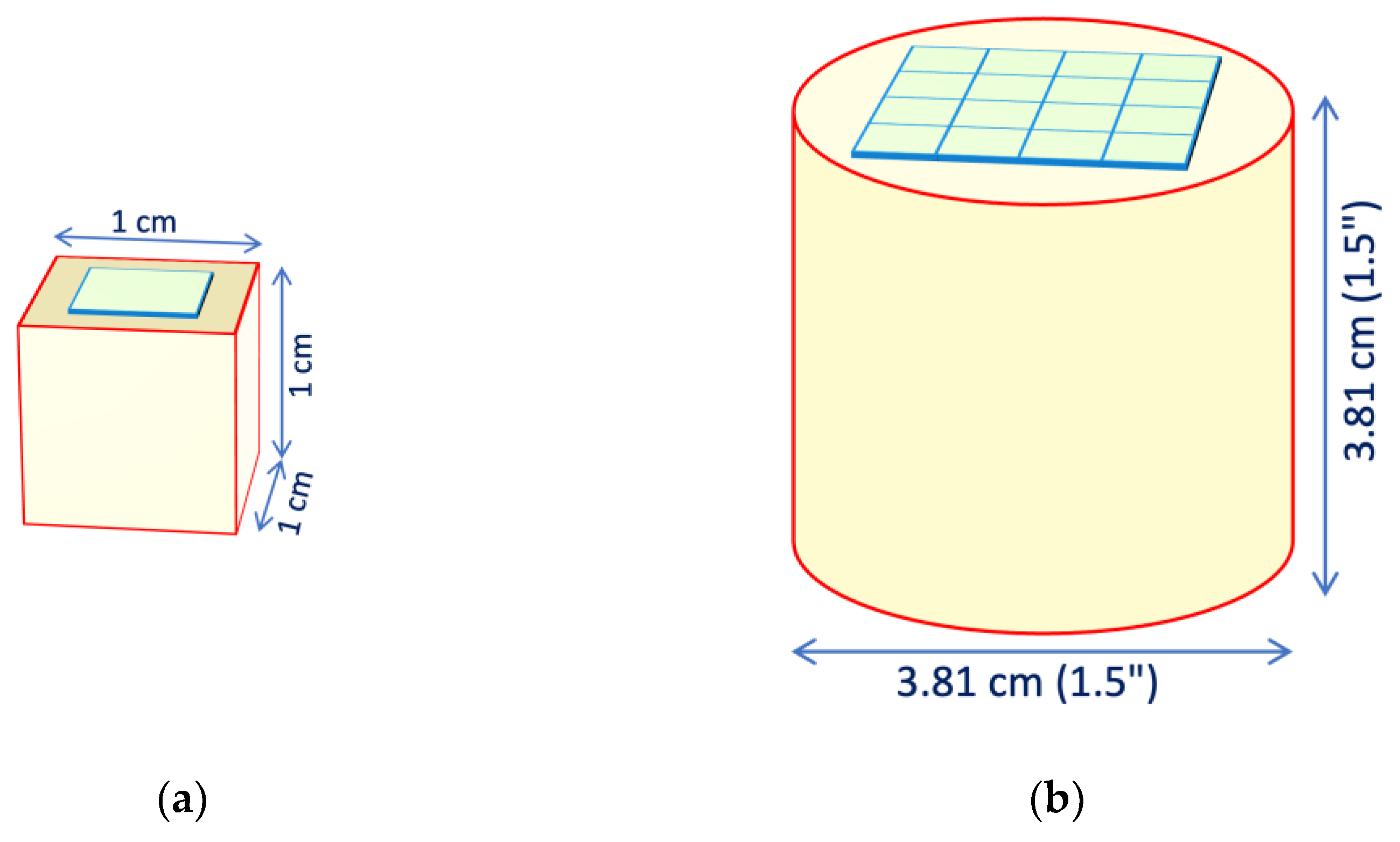
Figure 2.
Simulation of the light collection efficiency as a function of the reflectivity of the walls: (a) for the cubic configuration of Figure 1a; (b) for the cylindrical configuration of Figure 1b.
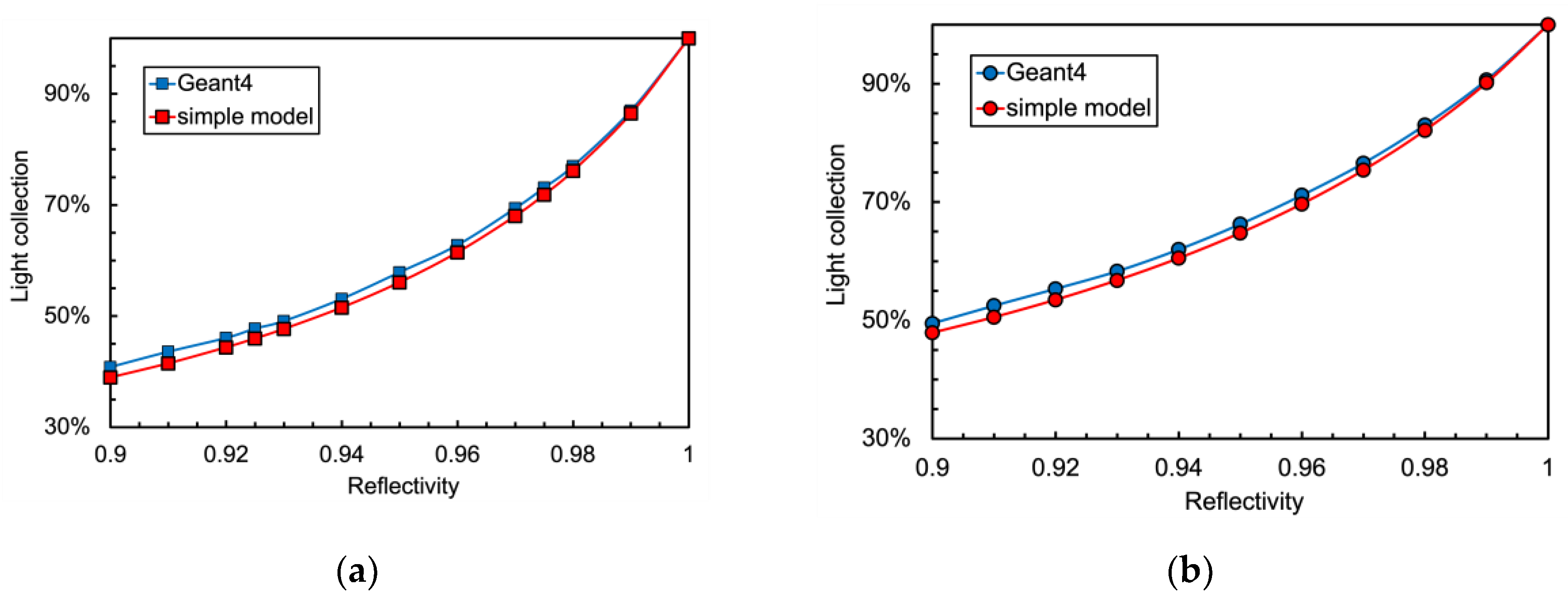
Figure 3.
Ratio simple-to-Geant4 between the curves of Figure 2: (a) Cubic configuration, also shown is the case of the empirically increased ε value. (b) Cylindrical configuration, also shown is the case of the empirically increased ε value.
Figure 3.
Ratio simple-to-Geant4 between the curves of Figure 2: (a) Cubic configuration, also shown is the case of the empirically increased ε value. (b) Cylindrical configuration, also shown is the case of the empirically increased ε value.
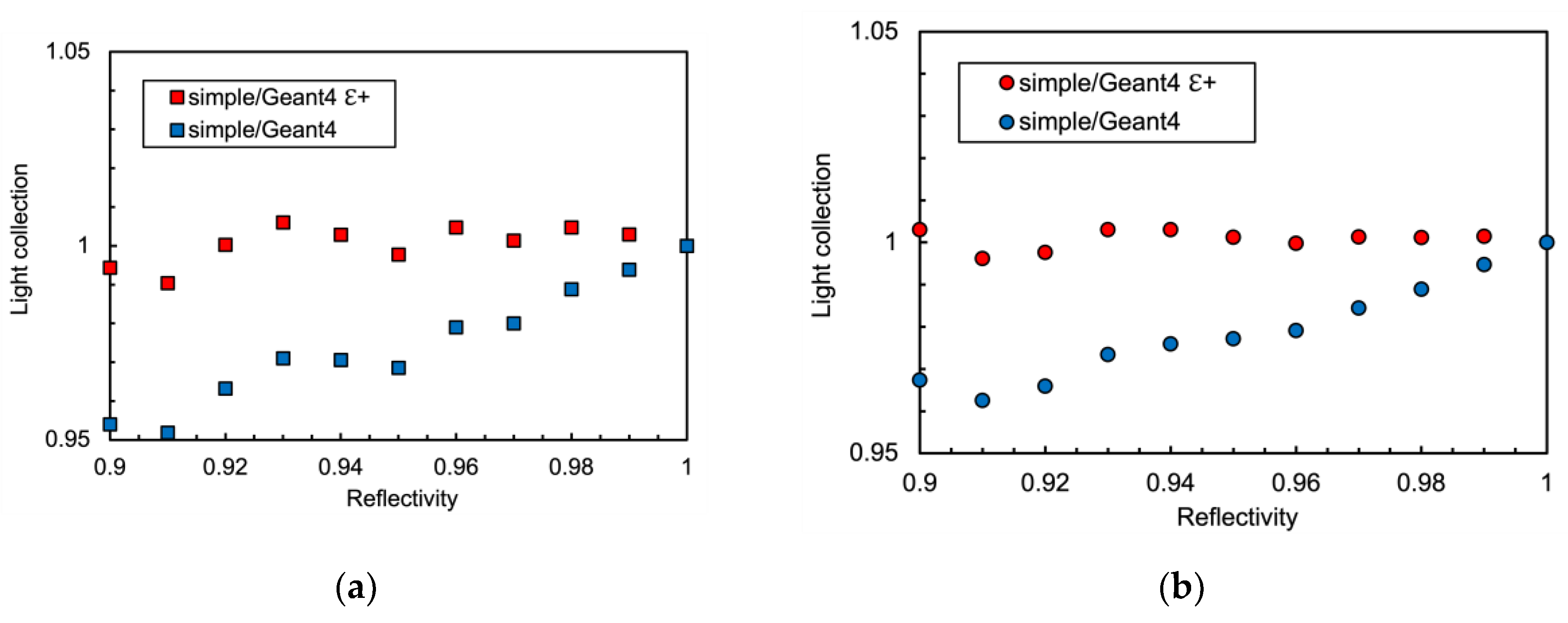
Figure 4.
Example of a signal waveform acquired from a CsI(Tl) scintillator coupled to a SensL SiPM in the configuration of Figure 1a with a digital scope. The exponential fit to the waveform has a decay constant of 0.96 µs as expected.
Figure 4.
Example of a signal waveform acquired from a CsI(Tl) scintillator coupled to a SensL SiPM in the configuration of Figure 1a with a digital scope. The exponential fit to the waveform has a decay constant of 0.96 µs as expected.
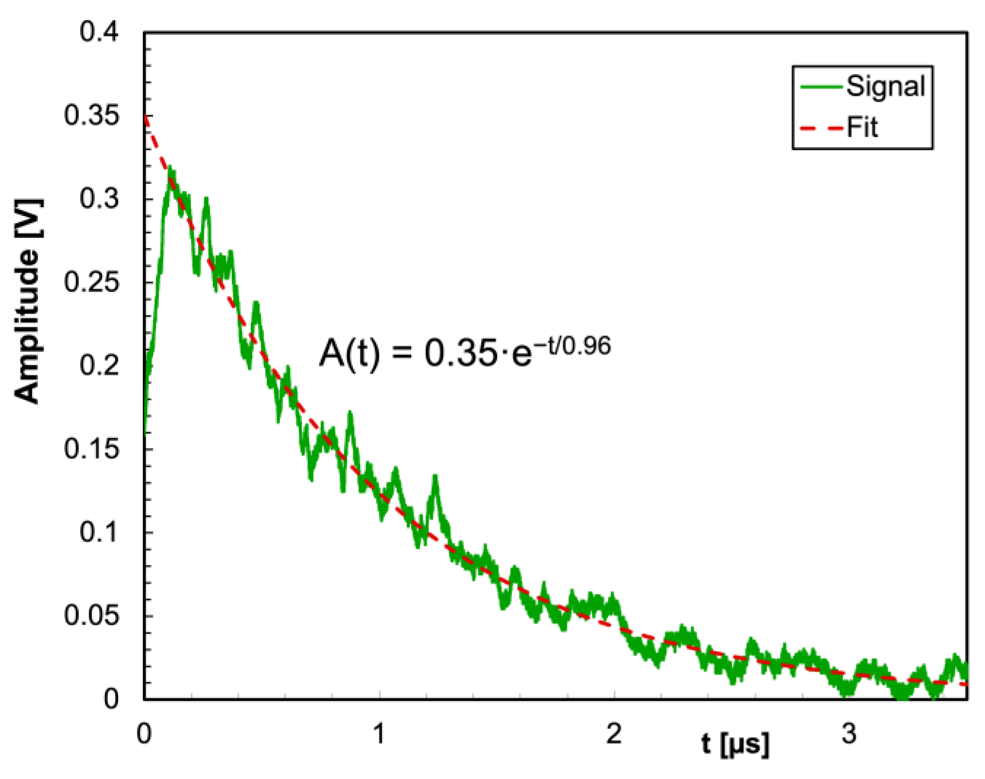
Figure 5.
The photon detection efficiency of the two SiPMs [17,18] (left scale), and the light emission spectra of the five scintillators normalized to unit area [19,20,21,22,23] (right scale).
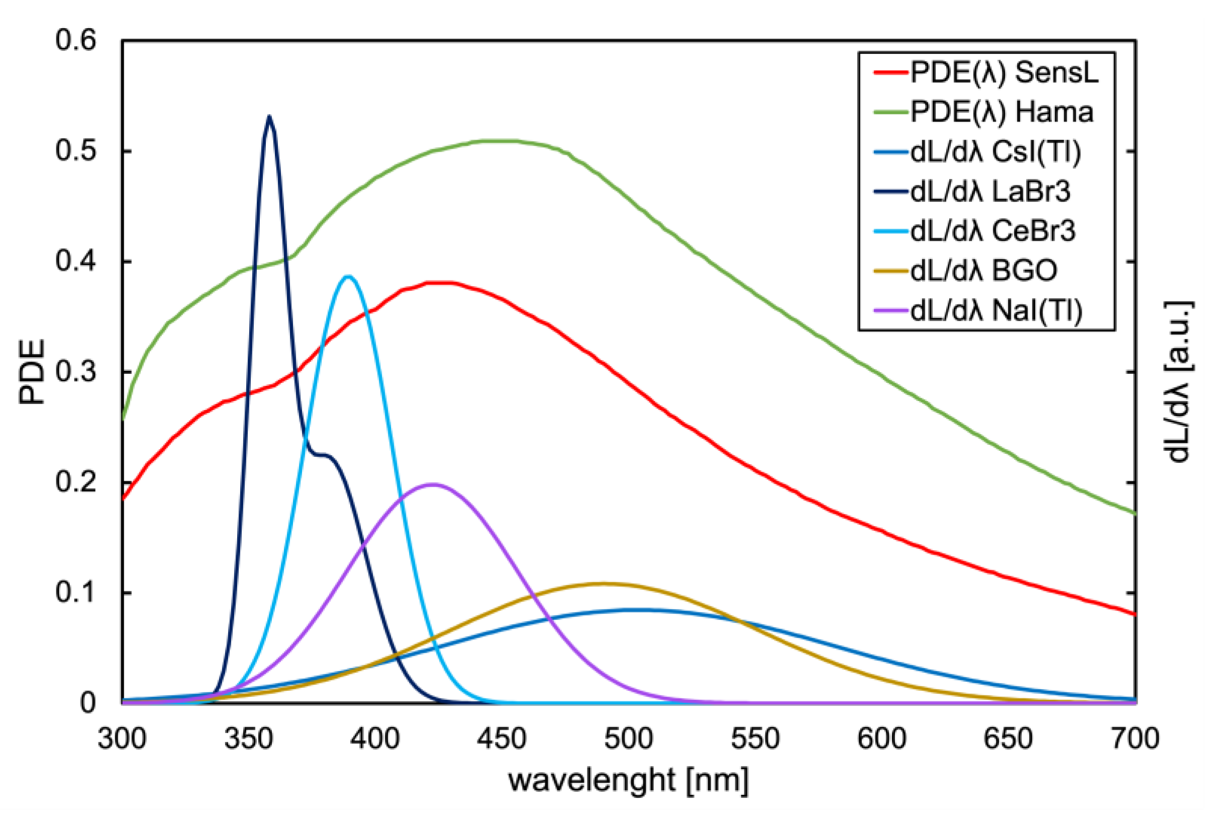
Figure 6.
Effective PDE of the two SiPMs when detecting the light emitted by each scintillator, calculate by integrating the product of the PDE(λ) function with the light emission spectrum.
Figure 6.
Effective PDE of the two SiPMs when detecting the light emitted by each scintillator, calculate by integrating the product of the PDE(λ) function with the light emission spectrum.
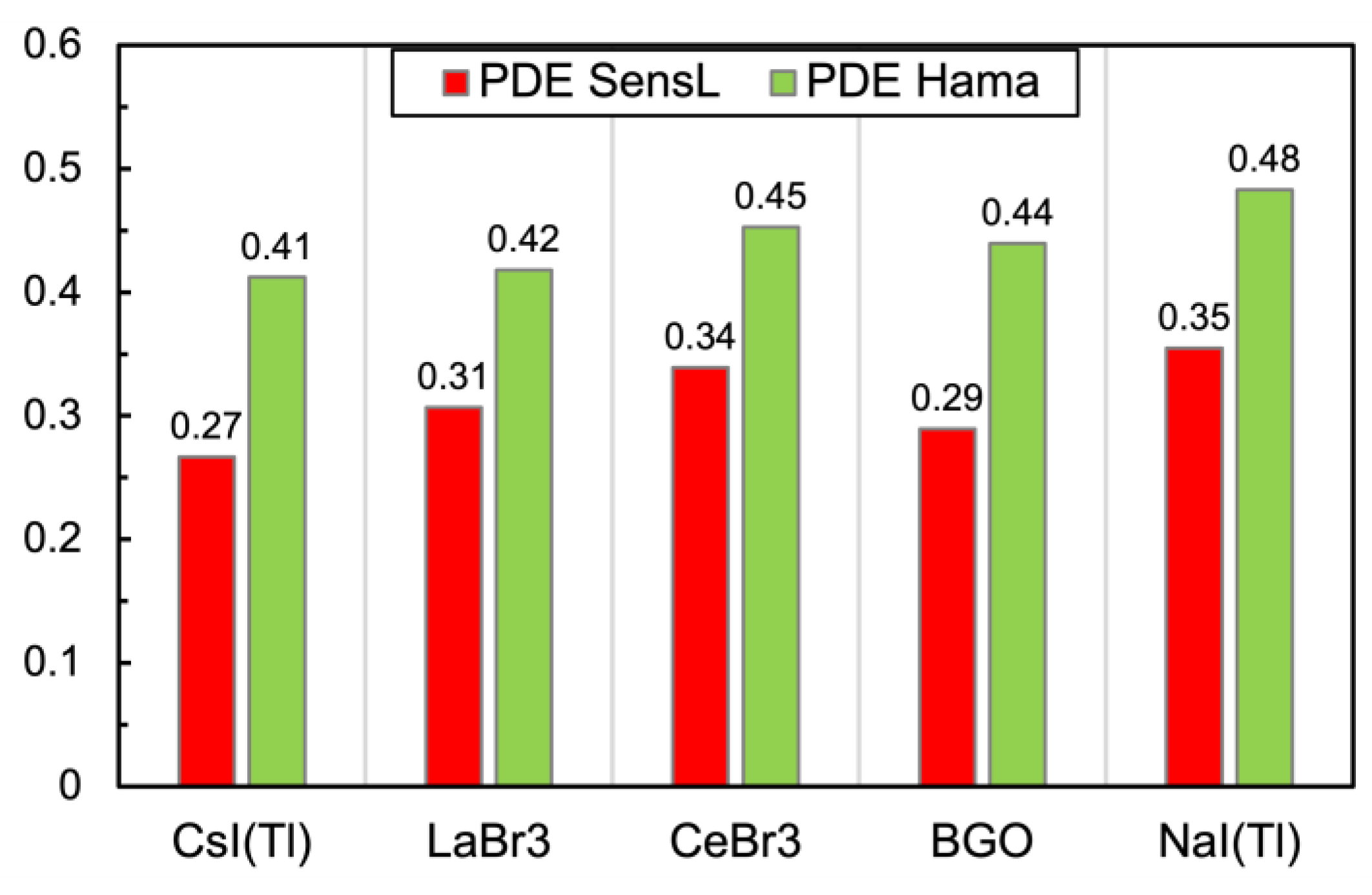
Figure 7.
(a) Time evolution of the number of triggered (dashed red line) and of available (green line, right-hand scale) microcells, for the case of 2 MeV deposited in a 1 cm × 1 cm × 1 cm CsI(Tl) crystal read by the SensL SiPM. The time step is 5 ns. Also shown is the ideal number of microcells (light blue line) that would be triggered if no recharge dead time were present. (b) Ratio between the number of fired microcells to the ideal one as a function of time.
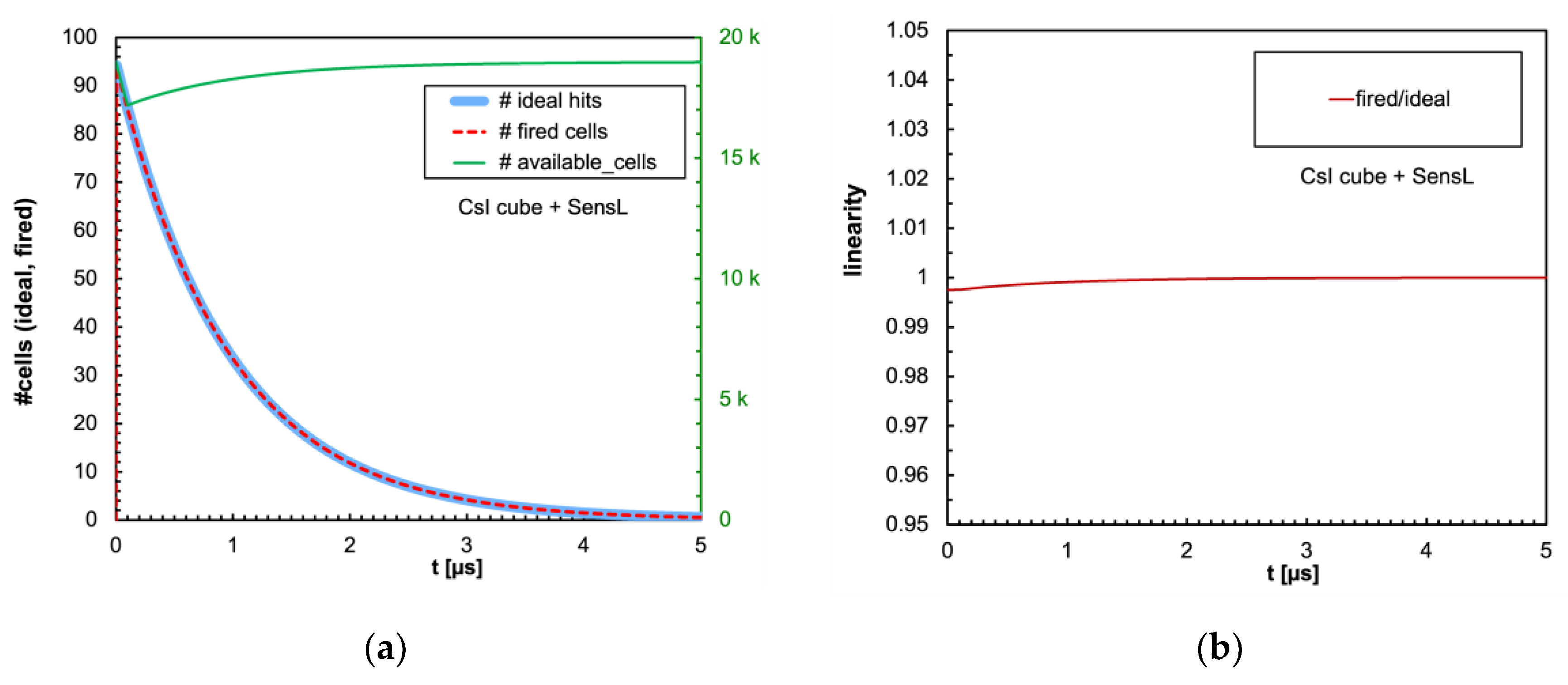
Figure 8.
(a) Same plot as in Figure 7a with the CsI(Tl) cubic crystal coupled to the Hamamatsu SiPM. (b) Same plot as in Figure 7b.
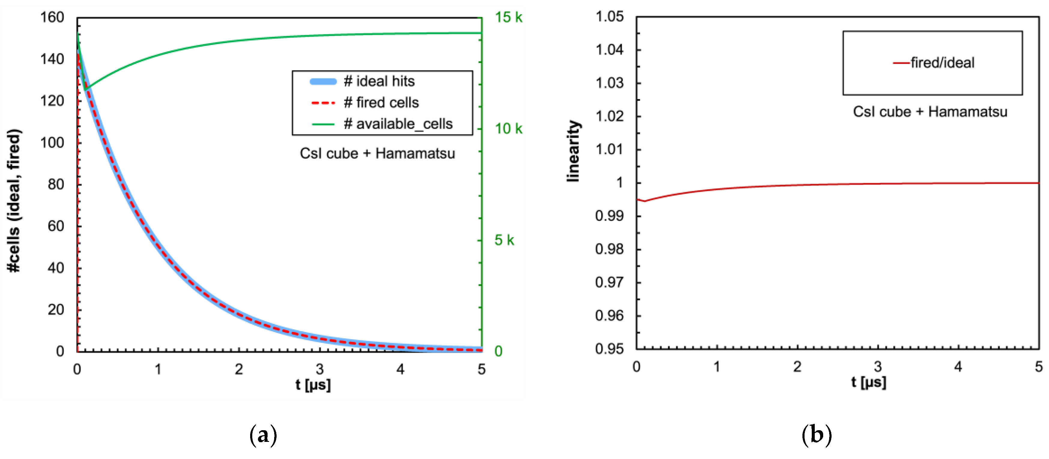
Figure 9.
(a) Same plot as in Figure 7a with the LaBr3(Ce) cubic crystal coupled to the SensL SiPM. (b) Same plot as in Figure 7b.
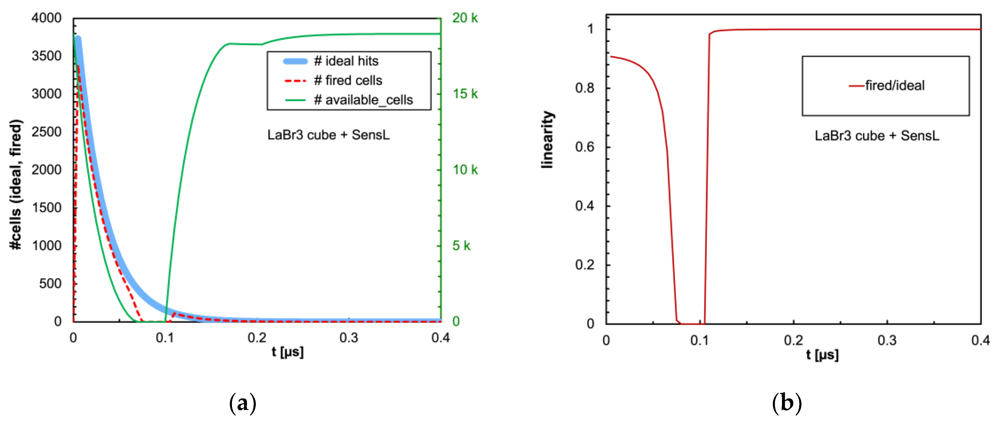
Figure 10.
(a) Same plot as in Figure 7a with the LaBr3(Ce) cubic crystal coupled to the Hamamatsu SiPM. (b) Same plot as in Figure 7b.
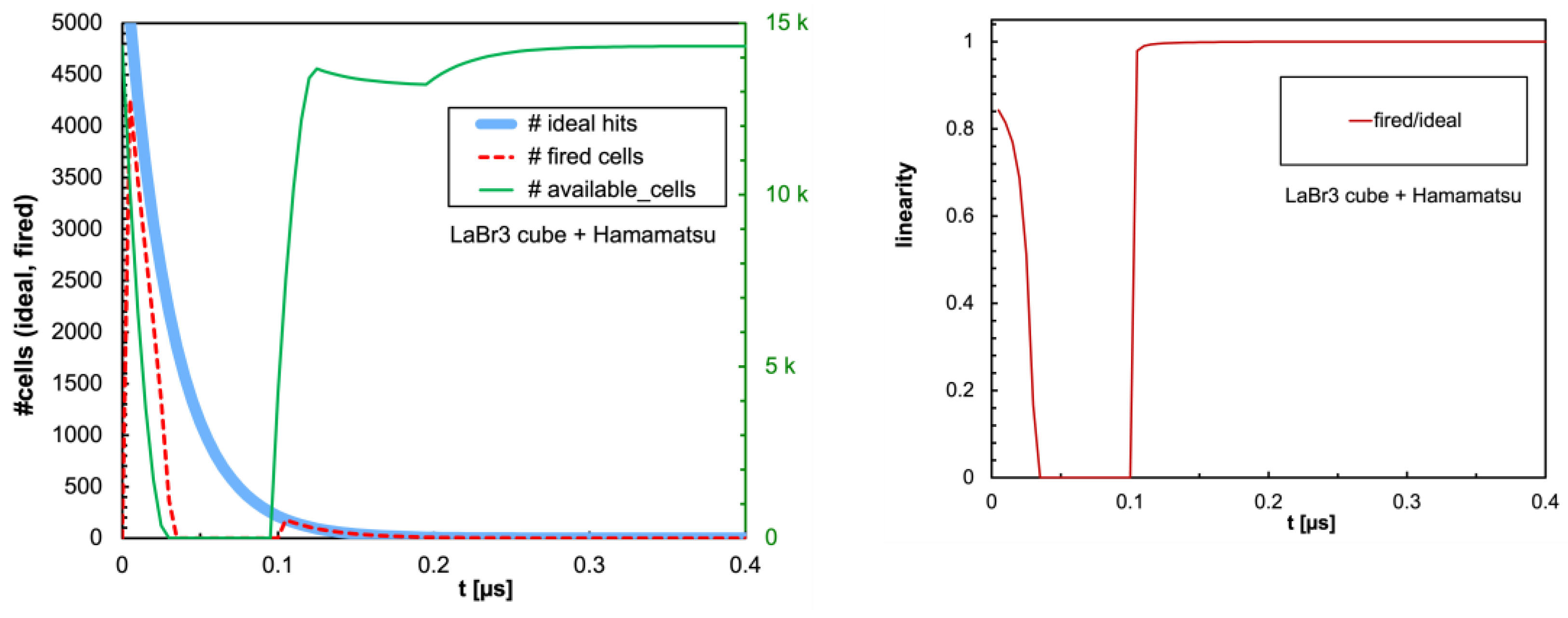
Figure 11.
(a) Same plot as in Figure 7a with the CeBr3 cubic crystal coupled to the SensL SiPM. (b) Same plot as in Figure 7b.
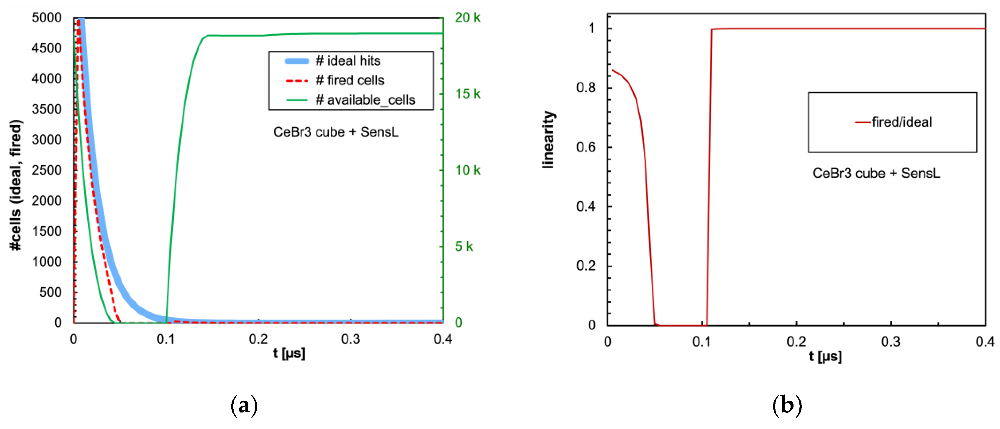
Figure 12.
(a) Same plot as in Figure 7a with the CeBr3 cubic crystal coupled to the Hamamatsu SiPM. (b) Same plot as in Figure 7b.
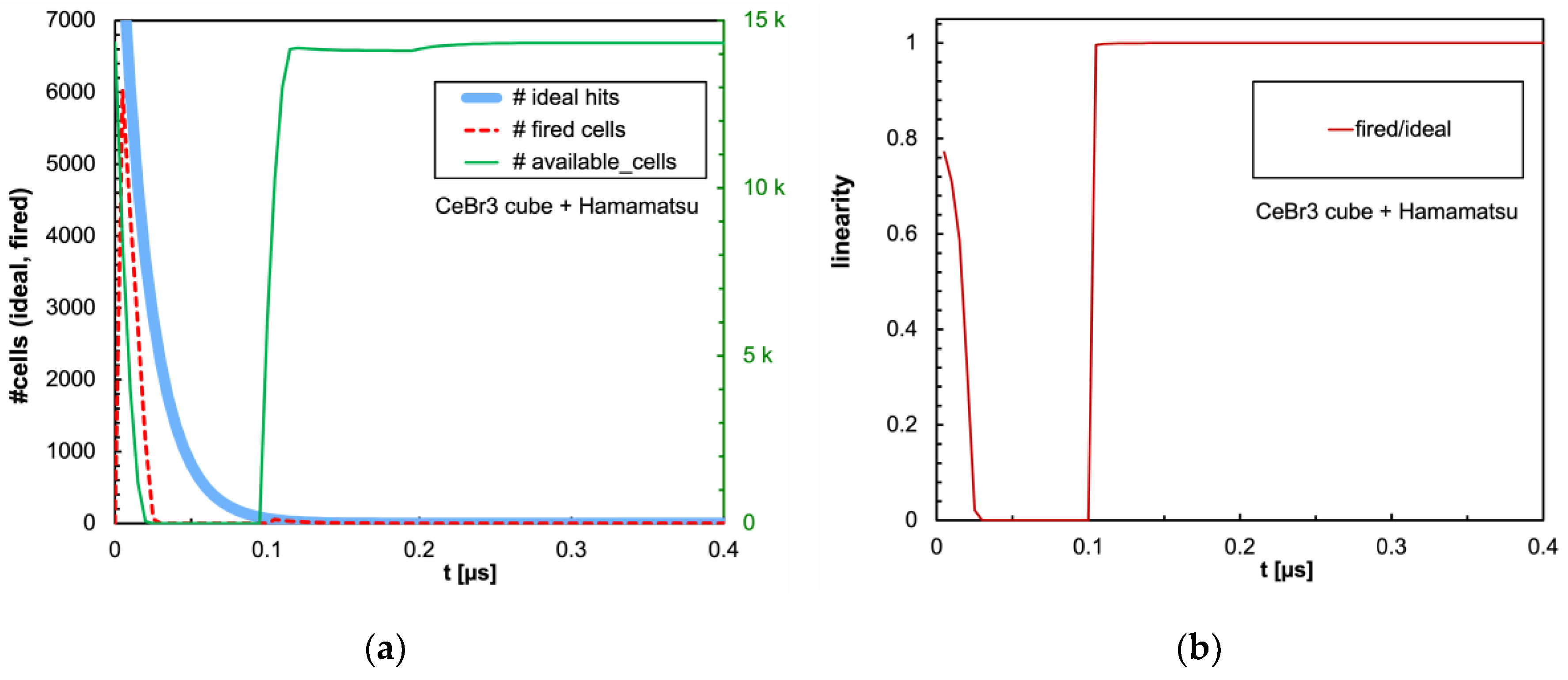
Figure 13.
(a) Same plot as in Figure 7a with the BGO cubic crystal coupled to the SensL SiPM. (b) Same plot as in Figure 7b.
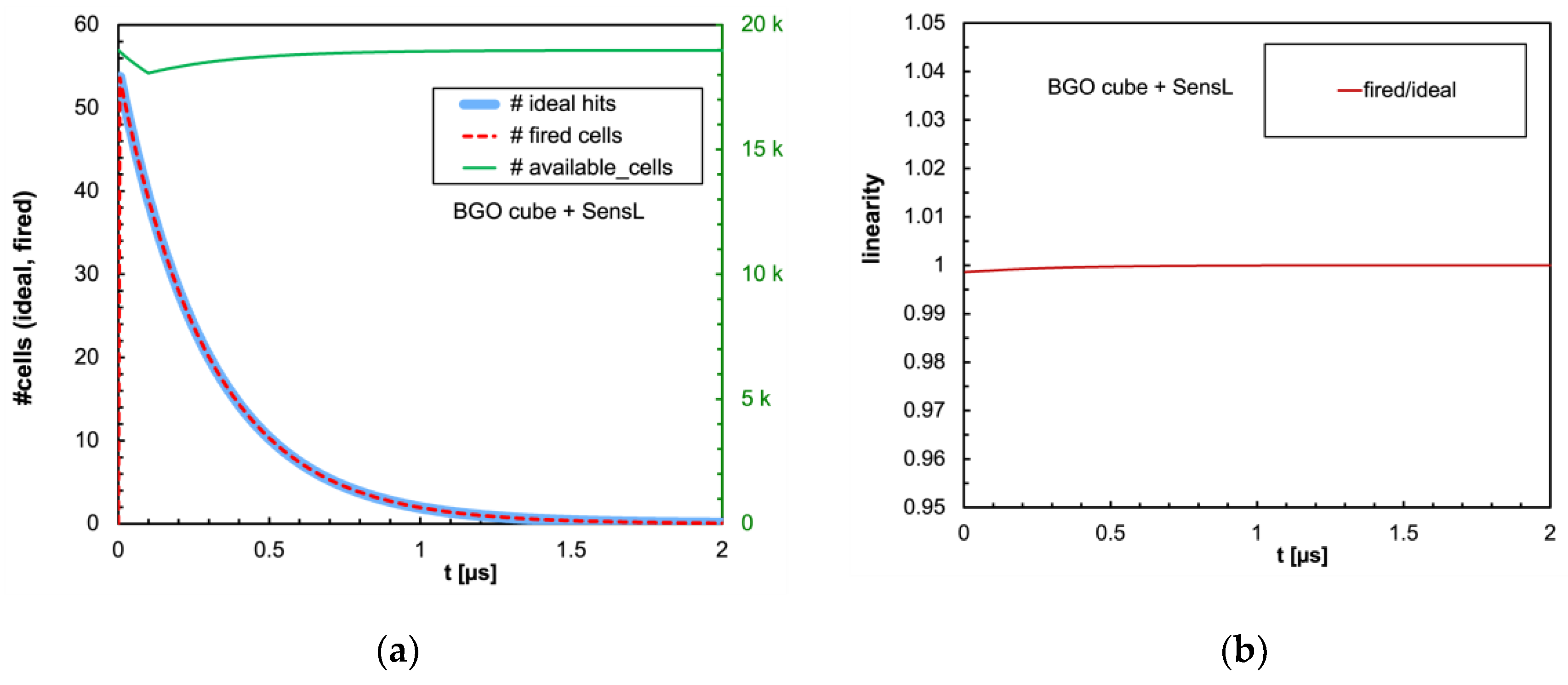
Figure 14.
(a) Same plot as in Figure 7a with the BGO cubic crystal coupled to the Hamamatsu SiPM. (b) Same plot as in Figure 7b.
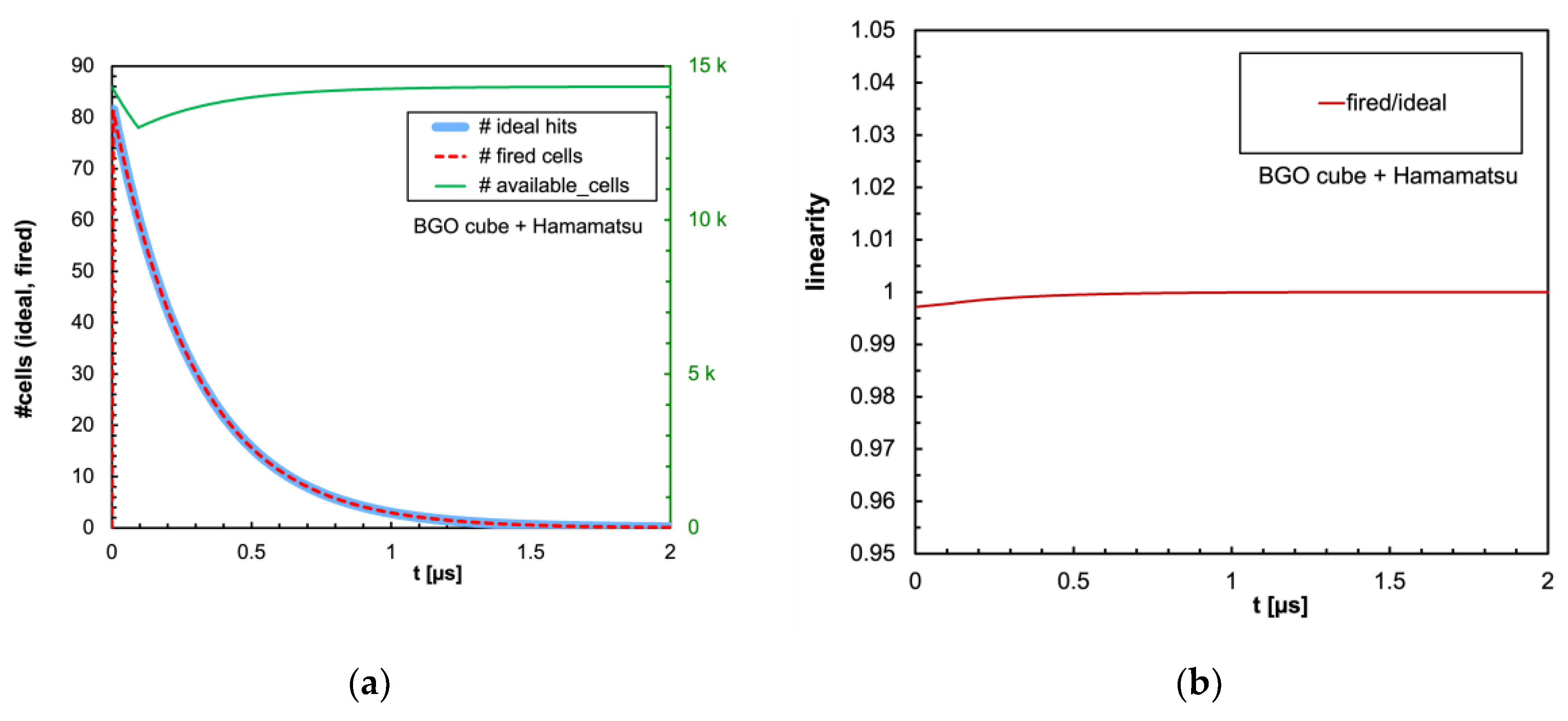
Figure 15.
(a) Same plot as in Figure 7a with the NaI cubic crystal coupled to the SensL SiPM. (b) Same plot as in Figure 7b.
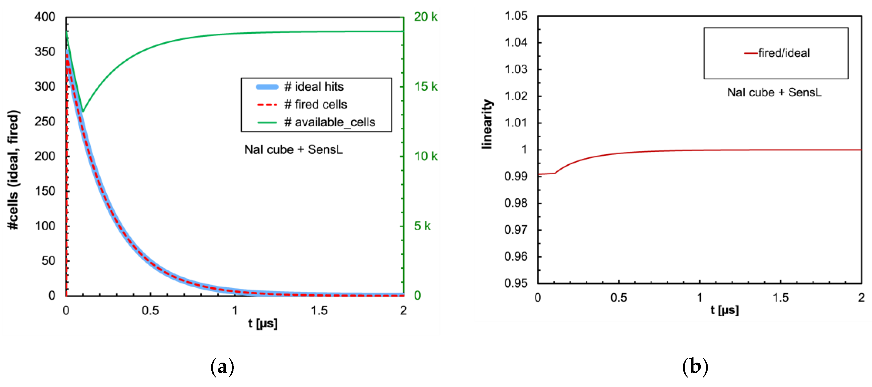
Figure 16.
(a) Same plot as in Figure 7a with the NaI cubic crystal coupled to the Hamamatsu SiPM. (b) Same plot as in Figure 7b.
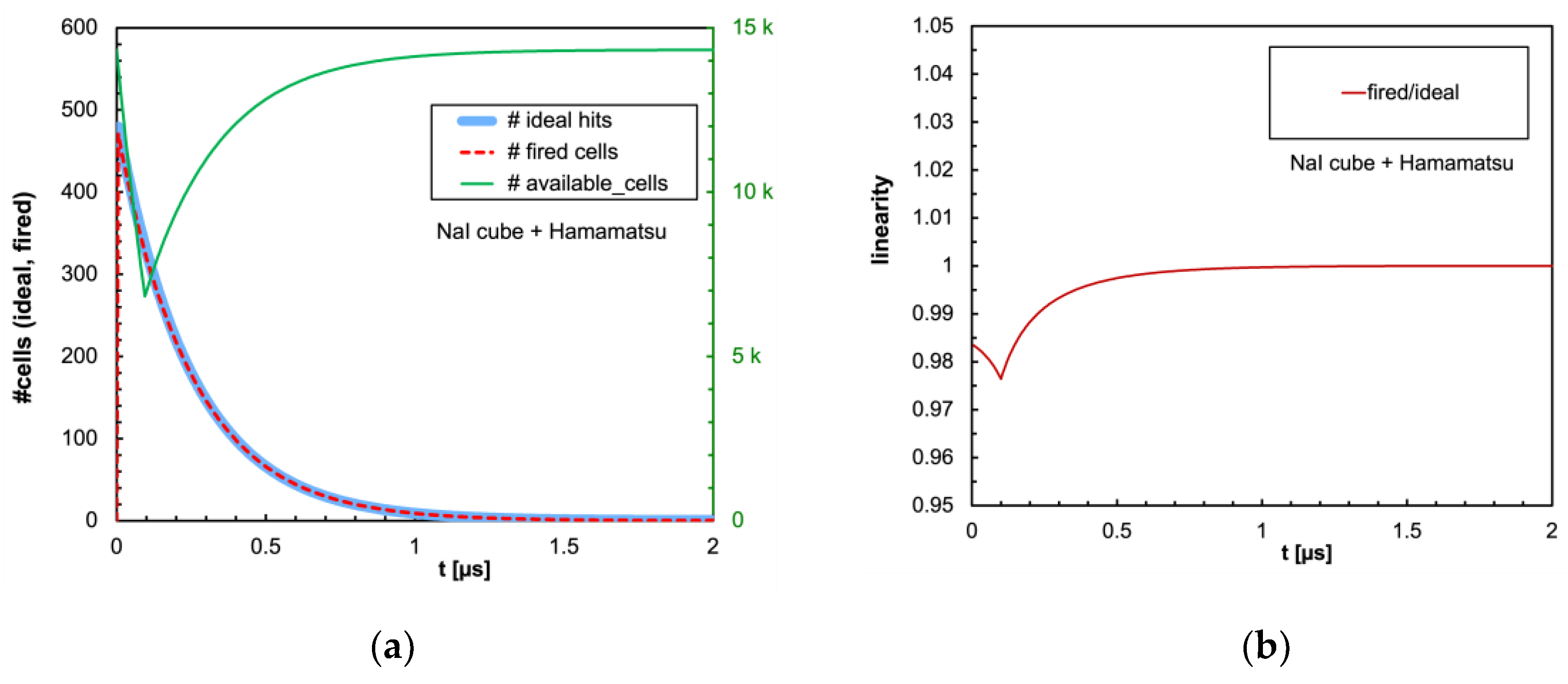
Figure 17.
Time-integrated results of the calculation with 2 MeV gamma energy deposited inside the five cubic scintillators. (a) Number of ideal hits and of actually triggered microcells for the examined configurations of scintillator and SiPM. (b) Expected non-linearity for each configuration.
Figure 17.
Time-integrated results of the calculation with 2 MeV gamma energy deposited inside the five cubic scintillators. (a) Number of ideal hits and of actually triggered microcells for the examined configurations of scintillator and SiPM. (b) Expected non-linearity for each configuration.
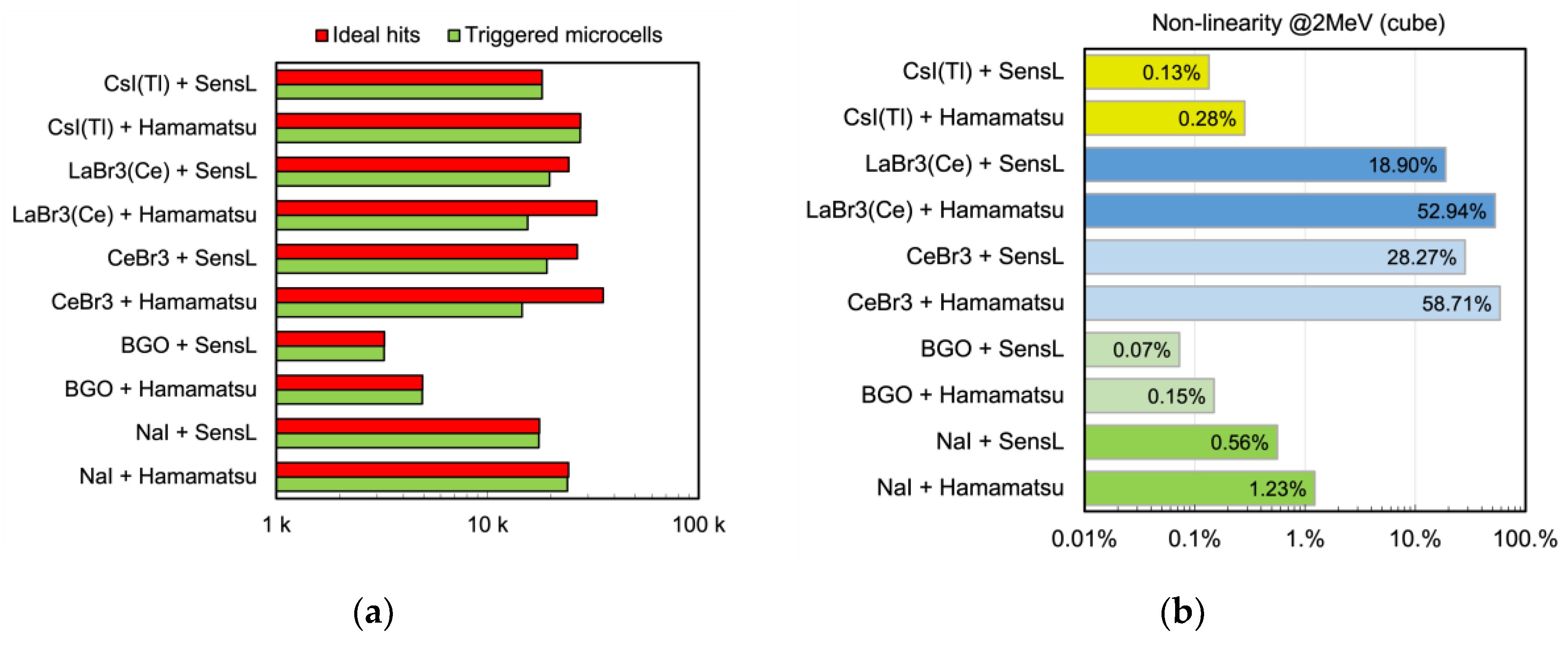
Figure 18.
(a) Time evolution of the number of triggered (dashed red line) and of available (green line, right-hand scale) microcells, for the case of 2 MeV deposited in a 3.81 cm × 3.81 cm cylindrical CeBr3 crystal read by the SensL SiPM. The time step is 5 ns. Also shown is the ideal number of microcells (light blue line) that would be triggered if no recharge dead time were present. (b) Ratio between the number of fired microcells to the ideal one as a function of time.
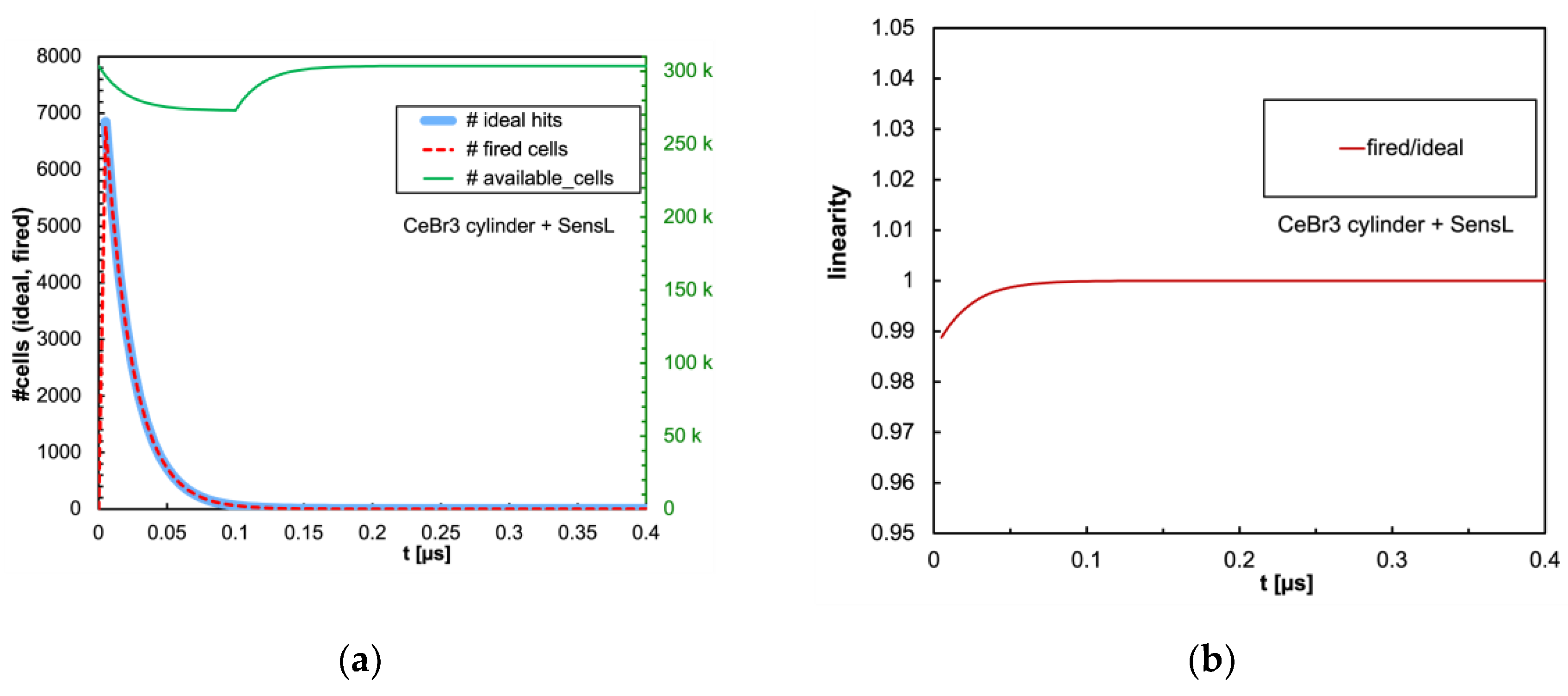
Figure 19.
(a) Same plot as in Figure 18a with the cylindrical CeBr3 crystal coupled to the Hamamatsu SiPM. (b) Same plot as in Figure 18b.
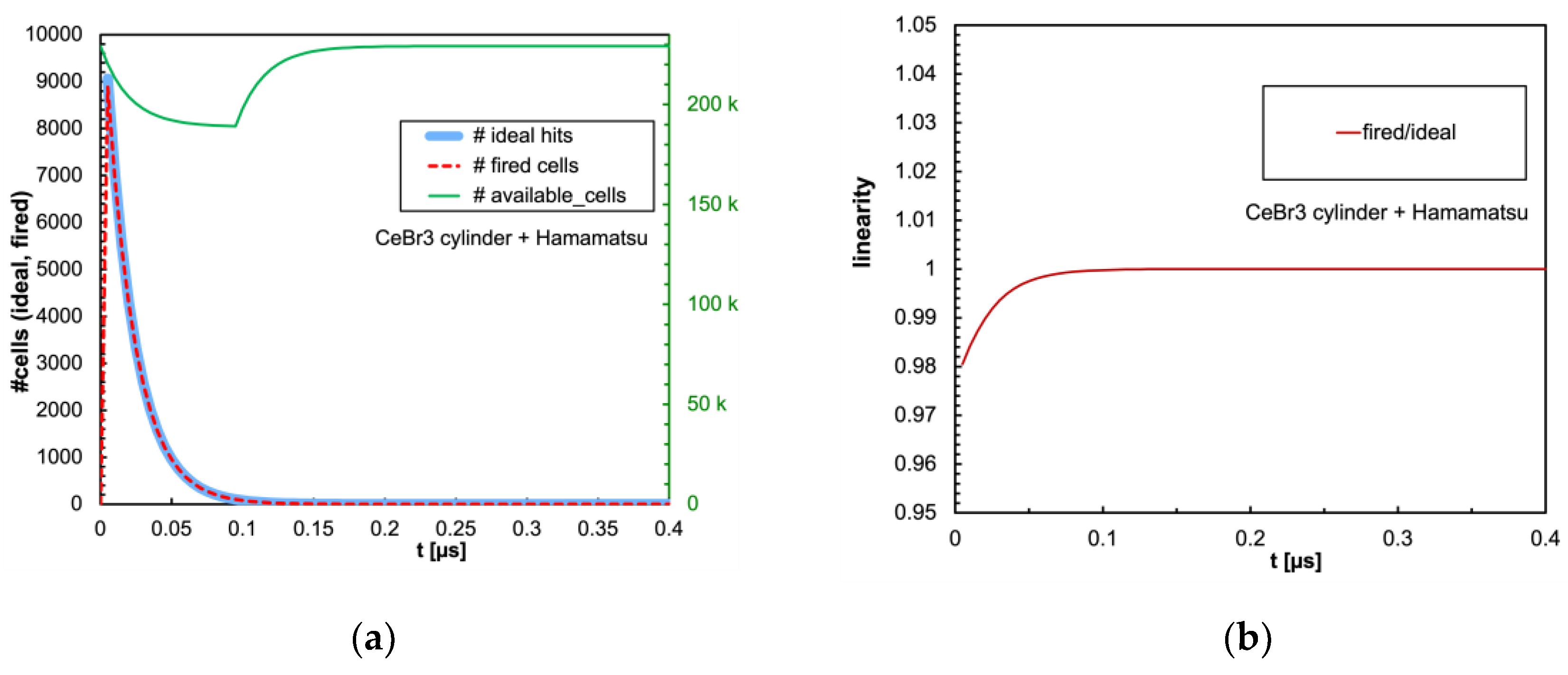
Figure 20.
Time-integrated results of the calculation with 2 MeV gamma energy deposited inside the five cylindrical scintillators. (a) Number of ideal hits and of actually triggered microcells for the examined configurations of scintillator and SiPM. (b) Expected non-linearity for each configuration.
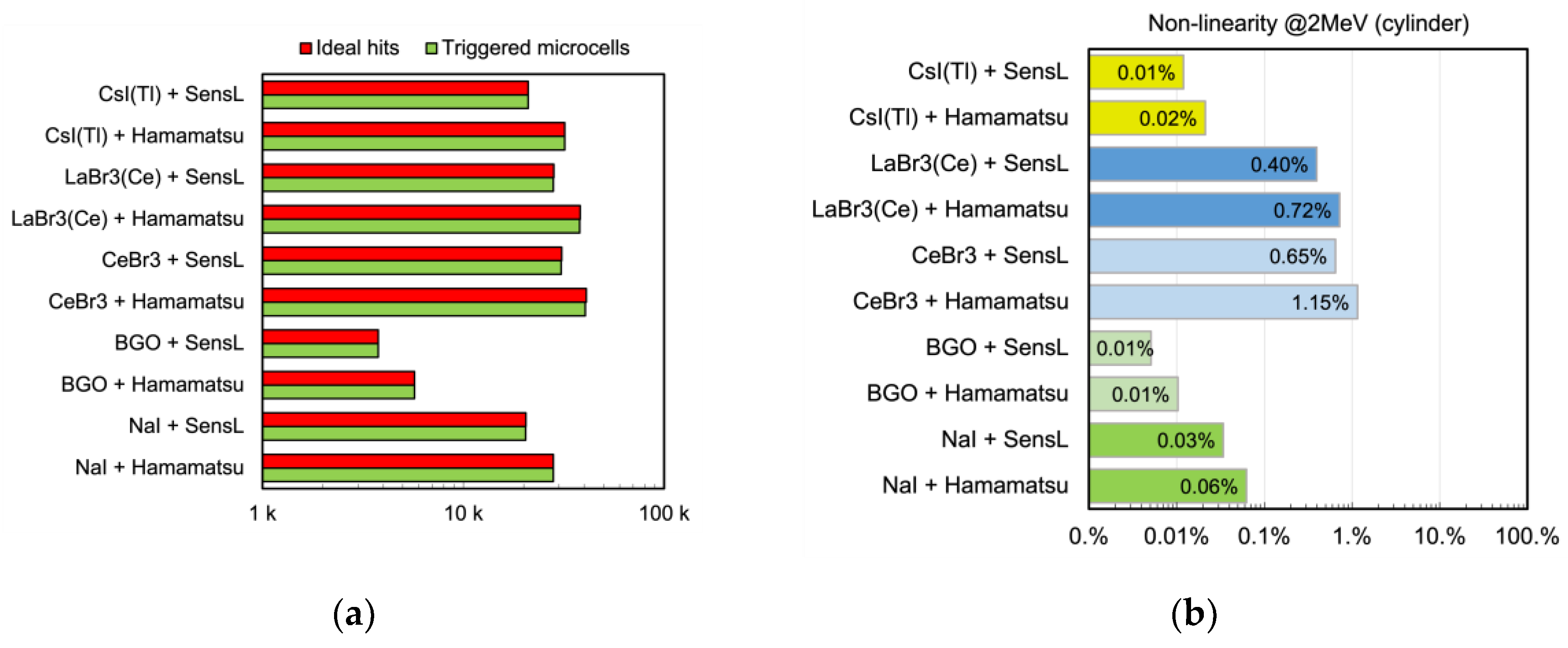
Figure 21.
Calculation of the total number of triggered microcells as a function of the gamma energy deposited inside a cubic scintillator of Figure 1a. (a) When coupled to a SensL SiPM. (b) When coupled to a Hamamatsu SiPM.
Figure 21.
Calculation of the total number of triggered microcells as a function of the gamma energy deposited inside a cubic scintillator of Figure 1a. (a) When coupled to a SensL SiPM. (b) When coupled to a Hamamatsu SiPM.
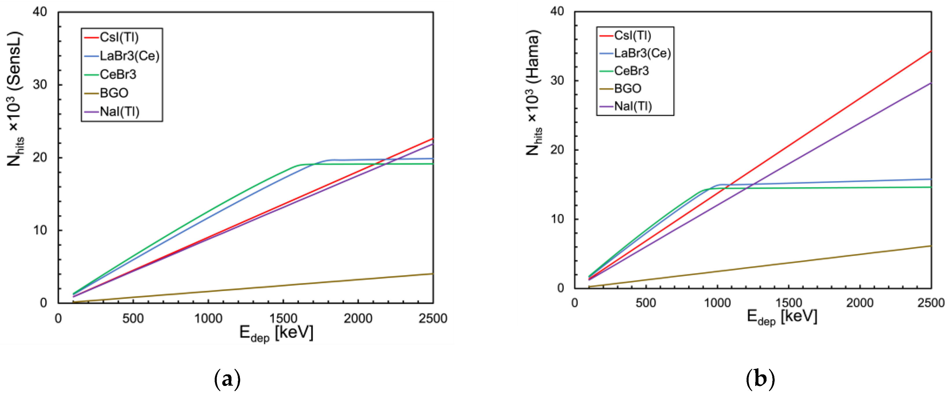
Figure 22.
Calculation of the total number of triggered microcells as a function of the gamma energy deposited inside a cylindrical scintillator of Figure 1b. (a) When coupled to an array of 16 SensL SiPMs. (b) When coupled to an array of 16 Hamamatsu SiPMs.
Figure 22.
Calculation of the total number of triggered microcells as a function of the gamma energy deposited inside a cylindrical scintillator of Figure 1b. (a) When coupled to an array of 16 SensL SiPMs. (b) When coupled to an array of 16 Hamamatsu SiPMs.
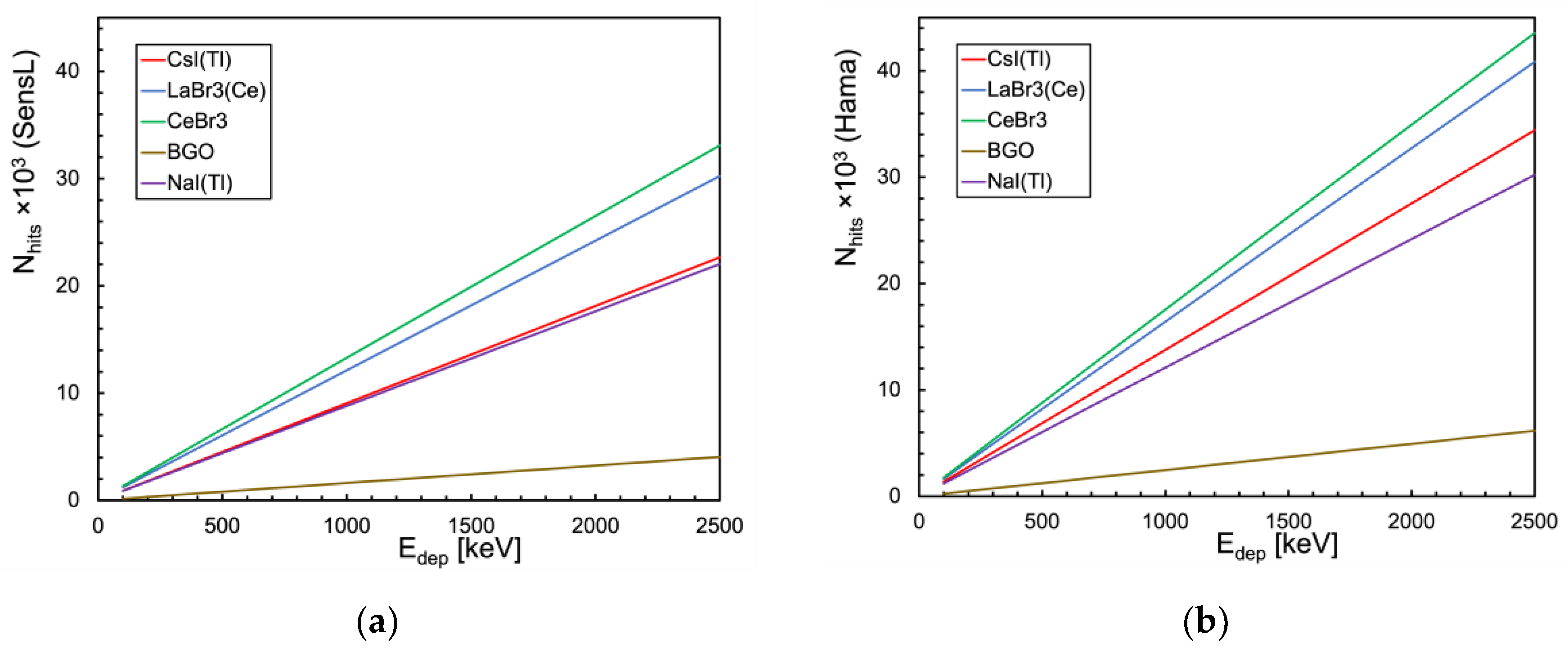
Figure 23.
(a) Spectra of four gamma sources acquired using a CsI(Tl) scintillator and a SensL SiPM. (b) The corresponding calibration plot. (c) Spectra of four gamma sources acquired using a CsI(Tl) scintillator and a Hamamatsu SiPM. (d) The corresponding calibration plot.
Figure 23.
(a) Spectra of four gamma sources acquired using a CsI(Tl) scintillator and a SensL SiPM. (b) The corresponding calibration plot. (c) Spectra of four gamma sources acquired using a CsI(Tl) scintillator and a Hamamatsu SiPM. (d) The corresponding calibration plot.
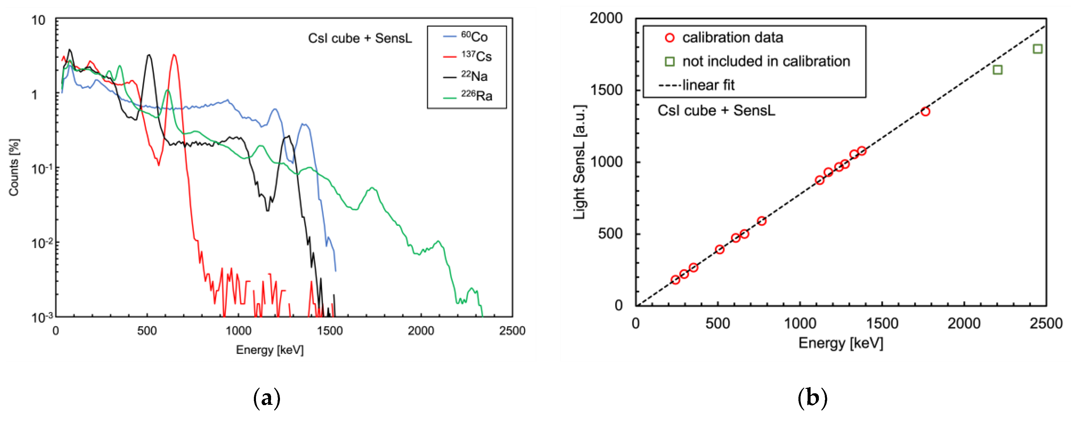
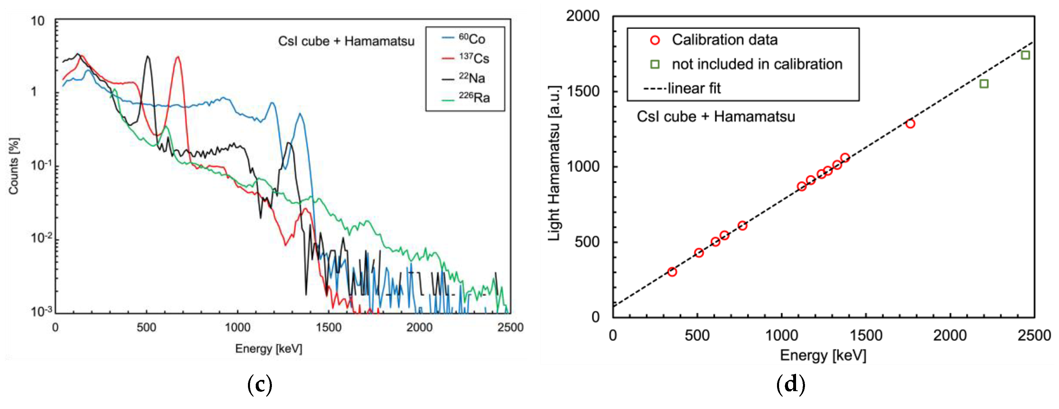
Figure 24.
Two additional detector geometries evaluated: (a) 1.5 cm × 1.5 cm × 1.5 cm scintillator coupled to a 2 × 2 array of 6 mm × 6 mm SiPMs; (b) 2.54 cm × 2.54 cm × 2.54 cm scintillator coupled to a 4 × 4 array of 6 mm × 6 mm SiPMs.
Figure 24.
Two additional detector geometries evaluated: (a) 1.5 cm × 1.5 cm × 1.5 cm scintillator coupled to a 2 × 2 array of 6 mm × 6 mm SiPMs; (b) 2.54 cm × 2.54 cm × 2.54 cm scintillator coupled to a 4 × 4 array of 6 mm × 6 mm SiPMs.
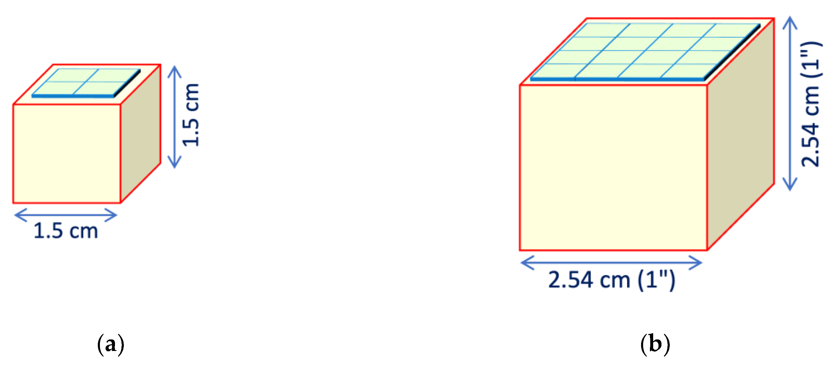
Figure 25.
Expected non-linearity at 2 MeV deposited energy for four geometrical configurations of LaBr3(Ce) and CeBr3 scintillators read by different arrangements of SensL and Hamamatsu 6 mm × 6 mm SiPM arrays.
Figure 25.
Expected non-linearity at 2 MeV deposited energy for four geometrical configurations of LaBr3(Ce) and CeBr3 scintillators read by different arrangements of SensL and Hamamatsu 6 mm × 6 mm SiPM arrays.

Table 1.
Main features, relevant to this study, of the selected five popular scintillators.
| CsI(Tl) | LaBr3(Ce) | CeBr3 | BGO | NaI(Tl) | |
| Light yield [photons/keV] | 60 | 70 | 70 | 10 | 45 |
| Decay time [ns] | 960 | 30 | 20 | 300 | 250 |
| Emission spectrum from ref. | [19] | [20] | [21] | [22] | [23] |
| Refractive index at λ max | 1.8 | 1.9 | 2.1 | 2.1 | 1.8 |
| Weighted PDE SensL [%] | 27% | 31% | 34% | 29% | 35% |
| Weighted PDE Hamamatsu [%] | 41% | 42% | 45% | 44% | 48% |
Table 2.
Main features, relevant to this study, of the two selected SiPMs.
|
MICROFC−60035−SMT SensL (now OnSemi) [17] |
S14160-6050HS Hamamatsu [18] |
|
| number of microcells | 18980 | 14331 |
| microcell recharge time [ns] | 100 | 92 |
Table 3.
Energy values of the peaks used in the calibration for each source. The first two were only used with the SensL equipped detector because of the large background. The two highest energy peaks from 226Ra, not used for the calibration, were used as a linearity cross check.
Table 3.
Energy values of the peaks used in the calibration for each source. The first two were only used with the SensL equipped detector because of the large background. The two highest energy peaks from 226Ra, not used for the calibration, were used as a linearity cross check.
| Gamma source | Peak energy [keV] | notes |
| 226Ra | 242 | only used with SensL |
| 295 | ||
| 352 | SensL and Hamamatsu | |
| 609 | ||
| 768 | ||
| 1120 | ||
| 1238 | ||
| 1377 | ||
| 1764 | ||
| 2202 | used for cross check and not for calibration |
|
| 2448 | ||
| 137Cs | 662 | SensL and Hamamatsu |
| 22Na | 511 | SensL and Hamamatsu |
| 1274 | ||
| 60Co | 1173 | SensL and Hamamatsu |
| 1330 |
Table 4.
FWHM energy resolution at 662 keV and non-linearity at 2 MeV for all the examined configurations. Notice that the resolution quoted here was naively calculated just for intercomparison as the inverse square root of the number of triggered microcells multiplied by 2.35.
Table 4.
FWHM energy resolution at 662 keV and non-linearity at 2 MeV for all the examined configurations. Notice that the resolution quoted here was naively calculated just for intercomparison as the inverse square root of the number of triggered microcells multiplied by 2.35.
| CsI(Tl) | LaBr3(Ce) | CeBr3 | BGO | NaI(Tl) | ||
| SensL + cube |
Resolution @662 keV | 3.03% | 2.65% | 2.54% | 7.17% | 3.08% |
| Non-linearity at 2 MeV | 0.13% | 18.90% | 28.27% | 0.07% | 0.56% | |
| Hamamatsu + cube |
Resolution @662 keV | 2.46% | 2.30% | 2.25% | 5.82% | 2.63% |
| Non-linearity at 2 MeV | 0.28% | 52.94% | 58.71% | 0.15% | 1.23% | |
| SensL + cylinder |
Resolution @662 keV | 3.03% | 2.62% | 2.50% | 7.17% | 3.08% |
| Non-linearity at 2 MeV | 0.01% | 0.40% | 0.65% | 0.01% | 0.03% | |
| Hamamatsu + cylinder |
Resolution @662 keV | 2.46% | 2.25% | 2.18% | 5.82% | 2.63% |
| Non-linearity at 2 MeV | 0.02% | 0.72% | 1.15% | 0.01% | 0.06% |
Table 5.
Summary of the main features of the evaluated detector configurations.
|
CeBr3 Hamamatsu |
LaBr3(Ce) Hamamatsu |
CeBr3 SensL |
LaBr3(Ce) SensL |
|
| cube size | 1 cm | |||
| n. SiPMs | 1 | |||
| n. microcells | 14331 | 18980 | ||
| sensor/total area ratio | 6% | |||
| collection efficiency | 56% | |||
| cube size | 1.5 cm | |||
| n. SiPMs | 4 | |||
| n. microcells | 57324 | 75920 | ||
| sensor/total area ratio | 10.7% | |||
| collection efficiency | 70% | |||
| cube size | 2.54 cm | |||
| n. SiPMs | 16 | |||
| n. microcells | 229296 | 303680 | ||
| sensor/total area ratio | 14.9% | |||
| collection efficiency | 78% | |||
| cylinder size | 3.81 cm | |||
| n. SiPMs | 16 | |||
| n. microcells | 229296 | 303680 | ||
| sensor/total area ratio | 8.4% | |||
| collection efficiency | 65% | |||
Disclaimer/Publisher’s Note: The statements, opinions and data contained in all publications are solely those of the individual author(s) and contributor(s) and not of MDPI and/or the editor(s). MDPI and/or the editor(s) disclaim responsibility for any injury to people or property resulting from any ideas, methods, instructions or products referred to in the content. |
© 2025 by the authors. Licensee MDPI, Basel, Switzerland. This article is an open access article distributed under the terms and conditions of the Creative Commons Attribution (CC BY) license (http://creativecommons.org/licenses/by/4.0/).
Copyright: This open access article is published under a Creative Commons CC BY 4.0 license, which permit the free download, distribution, and reuse, provided that the author and preprint are cited in any reuse.


