
Submitted:
07 September 2025
Posted:
08 September 2025
You are already at the latest version
Abstract
Modern utility systems were being heavily strained by rising energy consumption and dynamic load variations, which had an impact on the quality and reliability of the supply. Harmonic injection and reactive power imbalance were caused by the widespread divergence. Power quality (PQ) issues were mostly caused by renewable energy powered by power electronic converters that were integrated into the utility grid. Despite the fact that a range of industries required high-quality power to function properly at all times. Several solutions were frequently created, but continuing effort and newly improved solutions were needed to solve these problems by operating to various international standards. Distributed Static Compensator (DSTATCOM) was created in the proposed model to enhance PQ in a standard bus system. A standard bus system using the DSTATCOM model was initially developed. A real-time dataset was gathered while applying various PQ disturbance conditions. A deep learning controller was created using this generated dataset, which examined the bus voltages to generate the DSTATCOM pulse signal. Two case studies such as the IEEE 13 bus and the IEEE 33 bus system, were used to analyse the proposed work. Performance of the proposed deep learning controller was verified in various situations including interruption, swell, harmonics, and sag. The outcome of THD in IEEE 13 bus is 0.09% at the sag period, 0.08% at the swell period, 0.01% at the interruption period, and in IEEE 33 bus have 1.99% at the sag period, 0.44% at the swell period, 0.01% at interruption period. Also, the effectiveness of the proposed deep learning controller was examined and contrasted with current methods like K-Nearest Neighbour (KNN) and Feed Forward Neural Network (FFNN). The validated results show that the suggested method provides an efficient mitigation mechanism, making it suitable for all cases involving PQ issues.
Keywords:
power quality
; DSTATCOM
; IEEE 13 system
; deep learning controller
; IEEE 33 system
1. Introduction
Power Quality (PQ) has been a concern for both utility and end-user consumers over the past twenty years [1]. Interest in power electronics has grown quickly due to its widespread application in industrial processes, regulators, microprocessor-based devices, nonlinear loads, and the growth of computer networks. The quality of power delivered is also impacted by the grid integration of Distributed Generation (DG) technologies including wind, fuel cells, and solar photovoltaics [2]. PQ is the term for any variation in current, voltage, or frequency from their typical values that might lead to malfunctions or failures in user equipment [3]. PQ is related to many other types of disturbances, such as oscillatory and impulsive transients, voltage sag, voltage flicker, harmonics, multiple notches, and swell [4].
Several techniques have been suggested and put into use in order to lessen the system’s impact caused by voltage and power quality disturbances. The voltage differential between normal and disturbed operation circumstances is typically compensated for using custom equipment [5]. Recently, load balancing, reactive power compensation, and harmonic reduction have been implemented in the distribution system via the use of the Distribution Static Compensator (DSTATCOM) [6]. The performance of DSTATCOM is influenced by the control method utilized for the extraction of reference current components. Several scholars have proposed a variety of control techniques to accomplish this goal. These algorithms are based on a number of theories, including the ones on Instantaneous Reactive Power (IRP) [7], the Synchronous Reference Frame (SRF) [8], the Symmetrical Component (SC) [7], and the current compensation approach employing dc bus voltage regulation.
Afterward, some of the traditional controlling schemes were introduced to improve the power quality like Proportional Integral Differentiator (PID) [9], Proportional Integral (PI), fuzzy controller [10] and Fractional Order PID (FOPID) controller [11]. But, the ideal problem for these devices is challenging. In order to solve the problems with choosing the best parameters, an optimal controlling method is presented. Numerous optimal solving models were introduced for optimal parameter selection such as Particle Swarm Optimization (PSO) [12], and Atom Search Optimization (ASO). However, due to their long response times, high frequency noise, poor performance under parameter fluctuations, and difficult parameter tweaking, these approaches are not always effective. Artificial Intelligence (AI) is chosen to manage the compensator’s performance to get over these constraints.
AI methods are now widely used to solve a variety of power system issues, including forecasting, planning, scheduling, control, and more [13]. These solutions are able to perform difficult tasks in modern massive power networks with even more interconnections established to suit increased load demand. A regulating technique based on Deep Learning (DL) is created to enhance PQ in the distribution system in light of these advantages. A real-time dataset is generated under both normal and varied PQ problem conditions when the DSTATCOM model is integrated into a system. This dataset is used to construct the DL controller, which analyzes the system’s voltage ranges and generates the appropriate compensator pulsed to inject power for compensation. Enhancing a system’s power quality is necessary for safe and dependable operation. To enhance security, a well-designed controlling system is essential for managing the compensator’s operational condition. The following is a discussion of the planned work’s primary contribution,
- A standard bus system like IEEE 13 and IEEE 33 test bus system with DL based DSTATCOM model is designed to analyse various PQ issues scenarios.
- At the grid, a generator is chosen whose bus is regarded as PCC. In that system, a DSTATCOM compensator is connected.
- A real-time dataset is generated which contains three-phase bus voltages under normal and various PQ issues conditions.
- As per the obtained dataset, a Deep Neural network (DNN) controller is constructed and its trained model is integrated into the system.
- The controller analyses the voltage of each bus, every second and generates the appropriate pulse signal of the compensator. The proposed model mitigation process is validated in several circumstances like swell, sag, interruption and harmonics.
The following is the way the manuscript is set up: A few modern controlling techniques for enhancing PQ in a system with compensators are shown in Part 2. The operational process and numerical modeling of the compensator using the DL controller for improving PQ are explained in Part 3. The results and discussion are offered in Part 4, and the proposed model’s conclusions are found in Part 5.
2. Related Work
Mitigation of PQ issues in the distribution system is an essential for improving power quality in a system. According to the development of technology, several methods were developed to improve PQ in the distribution system. Some of the recently developed approaches were discussed as follows.
Prasad, et al. [14] had developed a Reduced Switch Count Multilevel Converter coupled with a PV system, a dc-link voltage of a DSTATCOM was optimized according to the requirement for load adjustment. The speedier and simpler hysteresis controller was employed to regulate the inverter switch gate pulses. However, it has a delayed transient reaction because of the hysteresis controller’s behaviour, which causes rippling dc-link voltage and renders it unstable for fast-changing loads. Badoni, et al. [15] had suggested a shunt compensator designed and implemented with an affine projection control technique to lessen PQ problems. The weighted values’ convergence served as the basis for the control approach, which was independent of the properties of the input signal. A working DSTATCOM prototype was created using a digital signal processor (DSP) and a three-phase voltage supply (VSC). Nevertheless, the models are not desirable choices because of their size, increased space requirements, gradual detuning, and potential for resonance load.
Kumar and Kumar [16] had developed a DSTATCOM to enhance the grid-connected PV system’s PQ. The online weight is determined by the ADALINE-based LMS controller based on the measured load current and the previous weights. However, there are downsides to these systems, including oscillation around the goal point, fixed perturbation steps, and limited efficiency in dynamic situations. Kanase and Jadhav [17] had suggested a Voltage Source Converter (VSC) reference signal by using an SRFT method to extract the necessary current components. DSTATCOM removed harmonics and reactive power from the three-phase distribution system using this technique. One of this model’s biggest flaws was its dependence on voltage feed-forward and cross-coupling blocks.
Pandu, et al. [18] had developed a DSTATCOM for neutral current compensation, load balancing, and the reduction of harmonics. To enhance power quality in the Local Distribution Grid, Recursive Least Square and the Interval Type-2 Fuzzy Logic Controller filter were used to generate switch signals for IGBT in DSTATCOM. The FLC cannot deduce knowledge or relationships from the system’s imprecise data, which is a disadvantage of utilising this paradigm. Babu and Malligunta [19] had suggested to enhance power quality in the power distribution system that provides high-quality power to consumers and load devices, a multilevel DSTATCOM configuration. The “PQ” based control approach creates a reference signal that was then further processed using a level-shifted multi-carrier PWM technique to produce gate pulses for a multi-level DSTATCOM structure. However, the usage of a high pass filter can result in undesirable phase shifts at some frequencies, as well as ripples in the passband or the stopband.
Hasanzadeh, et al. [20] had developed a STATCOM-based one-cycle controller to boost distribution network power quality. Switching pulses, a perfect control method, could be generated in STATCOM’s compensating switching design for a variety of goals. But this approach exhibits substantial inaccuracy in the response to the permanent state and poor response to the dynamic state, in addition to being extremely difficult to execute. Arya, et al. [21] had developed a D-STATCOM for the study of DS that was precisely positioned and scaled employing the gravitational search algorithm (GSA). IEEE 33 and IEEE 69 buses were utilized to test the algorithm’s efficacy. However, because reactive power modifies the voltage across the entire power system network, it jeopardizes the security of electrical networks.
Gopal and Sreenivas [22] had suggested a Voltage Source Converter (VSC)-based model for improving power factor, lowering harmonic, and eliminating voltage sags and swells utilising a Distribution Static Compensator This model simulates the IEEE 15 bus system, and it uses the sensitivity index to determine where the D-STATCOM should be placed within the test system. However, the model’s poor controlling performance rendered it unsuitable for actual application. Ahmed [23] had suggested an IEEE 14-bus system Flexible AC transmission system (FACTS) device for enhancing PQ. The system with STATCOM responds to voltage changes better than the system without STATCOM in terms of overshoot. The 3-phase voltage & currents d-q components are calculated using the PLL output. But because the model has poor regulating performance, it cannot withstand all conditions.
The above-mentioned literature presents several recently developed approaches aimed at improving power quality in electrical systems. While these models perform better in mitigating power quality (PQ) issues, they still exhibit several limitations. Some models are unreliable under fast-changing load conditions [14], while others demand more installation space, limiting their applicability in space-constrained environments [15]. Certain methods suffer from low efficiency under dynamic load conditions [16], and the use of cross-coupling blocks increases control complexity and can introduce stability issues, especially under dynamic conditions [17]. In addition, some approaches are very complex to implement [18], and the limited learning capability of Fuzzy Logic Controllers (FLC) restricts adaptability [19]. Other models show poor control performance [20], pose risks to power system security [21], and are unable to reliably maintain power quality under all grid scenarios [22]. Finally, some systems fail to ensure consistent performance in rapidly changing grid environments [23]. To overcome these issues, the proposed model used a compact Distributed Static Compensator (DSTATCOM) controlled by a deep learning-based system that automatically generated control pulses without complex structures or manual tuning. This approach improved stability, efficiency, and adaptability, effectively mitigating voltage sags, swells, interruptions, and harmonics.
3. Proposed Methodology
PQ improvement in the distribution side is considered as a significant task in the power system. Poor PQ causes several economic losses, interrupted power supply, and components misbehaviour. To maintain a constant power on the load side, several controlling system based FACTS devices were introduced, but the models had some limitations due to a poor parameter selection process. A controller based on DL has been developed recently to govern the efficiency of the compensator power injection. DL offers a wonderful alternative to classical machine learning, which depends on human experience. It can handle enormous amounts of data for small networks with a considerably reduced learning cost and can also adapt instantly to all data. So in the proposed model, advanced DL controller is designed to regulate the DSTATCOM for improving PQ in the distribution system.
Intelligent learning controller based DSTATCOM for the PQ improvement model is illustrated in Figure 1. At first, a standard bus system is designed based on the rule of IEEE standards. One of the generator is assumed as the grid supply in the designed bus system. The nearest bus of the grid is taken as a point of common coupling (PCC). A DSTATCOM is fixed at any location in a system, also an Energy Storage System (ESS) is linked to the DSTATCOM. A real-time implemented dataset is generated which contains voltage ranges of all busses at normal and PQ issues conditions. Based on this dataset, the DL controller model is designed and its trained model is fixed into the system. The DL model decides the power may inject or not from the energy storage system at the present period based on the trained model. The mathematical design of the proposed components are discussed as follows.
3.1. Modelling of STATCOM
Insulated Gate Bipolar Transistors (IGBT) are constant high speed switching elements used in DSTATCOM, a reactive power compensation device for diversion, with a control strategy based on “pulse-width modulation.” Through the use of energy loading devices at its input terminals, it may receive power from a DC energy source and generate and excite fully controlled reactive and real power at its output terminals. The equivalent diagram of DSTATCOM is shown in Figure 2.
The equation of the DSTATCOM terminal is stated as follows,
(1)
where, signifies shunt current and denotes shunt voltage. The real and reactive power exchanged with the system is stated as,
(2)
The reference compensator currents by , and are expressed as,
(3)
where, and , denotes the average load power, and are three-phase current. The power injected is given below equation,
(4)
The DSTATCOM injects the power based on the PWM signal of the switches. In order to inject enough power into the compensator to offset the load demand, an ESS is connected to it.
3.2. Voltage regulation of DSTATCOM
It is feasible to make by regulating the compensator’s current by including one in tandem with the load.
(5)
where, signifies compensator current, and denotes load current.
(6)
The fundamental workings of a DSATCOM are comparable to those of synchronous machines. When underexcited, the synchronous machine will produce lagging current; when anxious, it will produce a leading current. Similar to synchronous machines, DSTATCOM may produce and absorb reactive power. If an external device is connected to it, it may exchange real power. DC power supply.
Exchange of reactive power- When the voltage source converter’s voltage output exceeds the system voltage, the DSATCOM functions as a capacitor and produces reactive power.
Exchange of real power- The DC capacitor is necessary to give the switches the necessary actual power because the switching devices cannot be lossless. For direct voltage management, actual power exchange to an AC system is therefore required to maintain a constant capacitor voltage.
Reactive power correction keeps the source current at unity power factor (UPF) by supplying reactive power as required by the load using DSTATCOM. Load balancing is accomplished by balancing the source reference current because the source is the only source of power. The true basic frequency component of the load current is present in the reference source current, which is utilized to determine when to switch on the DSTATCOM. The most crucial aspect of DSTATCOM control is the generation of appropriate PWM firing, which has a significant influence on both steady state and transient performances as well as compensating objectives. The suggested approach uses a DL-based controller to create a PWM signal in a compensator so that the power supply remains constant while the load is being operated.
3.3. Modelling of DL controller
Deep learning based controlling system of the compensator is discussed in this section. Deep learning (DL) teaches computers to learn from examples in the same way that people do. A computer may build a hierarchy of complicated concepts from smaller ones by using layer-based learning. So in the proposed model deep learning based controlling system of DSTATCOM is developed to improve PQ in the distribution system. Here, a deep neural network (DNN) is preferred to analyse the voltage and produce a suitable PWM signal to a compensator. The numerical expression of the proposed controller is stated as follows.
3.4. Modelling of DNN controller
In the proposed model, a dataset is created as per the real-time simulation analysis. On the basis of the generated dataset, the intelligent controller is constructed. In this case, the DNN is made to produce the proper pulse signal for the compensator. The key advantage of employing this controller is its capacity to bridge extremely long time lags without the need for fine modifications due to its constant error back propagation between memory cells. The voltage of each bus is sent as the input to the DNN, and the output is the pulse signal of the compensator at that time.
3.5. Working process
A DNN is a system of neurons organized in layers, where each layer processes simple calculations and receives input from the layers above it. The layers are made up of nodes that are just locations where computation takes place. For each pair of units in every two-layer succession, there is a difference in the bias and weight of every node. The output layer, input layer, and hidden layer are the three stages that comprise a DNN. The DNN input layer receives the given input data. Thirteen distinct sources provide input to the proposed model’s input layer. The input data is processed mathematically by the DNN hidden layer. There are a lot of hidden layers in DNN. The final layer, also known as the output layer, has a direct connection to the desired outcome that the model is trying to predict. The architecture of DNN is shown in Figure 3.
Let’s consider, the number of inputs are ; is hidden layers k differs from 1, 2, , n ; the hidden neuron bias, and denote weight of the layer.
The general form of the input layer is,
(7)
Taking into account a DNN with three hidden layers, the term for network computing with three hidden layers is,
(8)
(9)
(10)
The general phrase for a hidden layer is,
(11)
The following equation is computed as the output,
(12)
Where is bias, is refers to input units, is the input, is units in the hidden layer, is the output unit, and is the activation function. Using this DL controller to generate the pulse signal of a compensator.
4. Result and Discussion
The purpose of the proposed DL controller-based DSTATCOM model is to validate its efficacy under the different conditions are covered in this part. Initially, a standard bus system with a DSTATCOM model is designed, at this period the bus voltages are collected and named as normal condition. Then applying various kinds of faults in the system to generate PQ issues, at each period the bus voltages are collected and named individually. The collected bus voltages are termed as real-time dataset, as per this dataset the proposed DL controller is designed. Each second the proposed controller analyses the bus voltages and produces a parallel PWM signal of DSTATCOM. The proposed model was designed and the performance was validated using MATLAB/Simulink 2021b software. The performance analysis of the proposed model is validated under two conditions namely,
Case 1: Performance analysis in IEEE 13 bus system
Case 2: Performance analysis in IEEE 33 bus system
Each case is examined separately, and the results are given in the sections that follow. In each scenario, the suggested controller efficiency is validated in several circumstances like sag, interruption, swell, and Total Harmonic Distortion (THD) content. Table 1 demonstrates the designing parameter of STATCOM.
Table 2 contains the parameter that was utilised to create the proposed and present controller designs.
Dataset generation
The generation of the dataset, which is a crucial step for PQ mitigation, comes first in the suggested paradigm. A standard IEEE bus model with DSTATCOM is developed and collects each bus voltage without altering any of the factors that are taken into account for normal system data. Apply a fault to the system next to make it sag in a similar manner swells and interruptions are made in the system to gather data. The categorized collected datasets are saved in an excel file.
Designing the DNN controller that generates the pulse signal for the IGBT of DSTATCOM by uses this real-time dataset. The suggested controller analyses the bus system voltage once in every second and produces a suitable pulse for the switches. In this manner, dataset for a bus system is produced, and its PQ mitigation effectiveness is examined. Table 3 demonstrates the overall samples of the dataset and its attributes.
The voltage data used for training and testing the deep learning-based DSTATCOM controller were collected at a sampling rate of 10 kHz, which provides adequate temporal resolution to capture transient events and high-frequency components commonly associated with power quality disturbances. For each type of disturbance voltage sag, swell, and interruption a fault duration of 0.2 seconds was used within a 1-second simulation window. This time frame ensures that the controller can detect and react to PQ events promptly. This fault injection helps the controller learn to operate effectively under variable and imperfect conditions that are typically found in practical utility environments.
4.1. Case 1: Performance analysis in IEEE 13 bus system
In this case, the effectiveness of PQ mitigation is analysed using the IEEE 13 bus system. The suggested controller-based DSTATCOM is intended to be kept in the bus system and its mitigation process has been examined in the issues of sag, swell, and interruption. Additionally, its THD was examined both before and after compensation.
4.1.1. IEEE 13 bus system
This executed simulations based on the IEEE-13 bus test feeder to analyse the impact of DSTATCOM on PQ concerns in distribution systems. This system is comprised of a single generation unit, a voltage regulator unit consisting of three single-phase units linked in a wye, a main transformer ∆-Y to 115/4.16 kV (substation), an in-line Y-Y transformer to 4.16/0.480 kV, scattered, two shunt capacitor banks, and unbalanced loads, and thirteen buses via ten lines [24]. This bus system is used to analyse the sag, swell, interruption, and THD, which are all discussed in the section below.
Sag issues
The voltage drops by 10% of the nominal voltage during the short instant when the waveforms collapse. Every bus voltage is transmitted to the proposed controller, which analyses the input voltages (39 attributes) and produces the appropriate DSTATCOM pulse signal. Bus number 4 develops a sag fault, which lowers the voltage for a short period of time.
The compensator injects voltage to make up for the voltage in the load during a sag event, which occurs when the voltage falls below the nominal value. The voltage waveforms for the proposed model are shown in Figure 4 during the sag period. That causes the sag problems to occur between 0.25 and 0.5 seconds. DSTATCOM injects voltage throughout that time, allowing the load voltage to be adjusted and a steady power flow to be maintained. Figure 5 analyses and plots the THD data for the load side. THD is a measure of signal distortion that assesses the energy contained in the harmonics of the original signal. According to the graphical model, the load side’s THD value after correction is 0.09%.
Swell issues
Sag compensation is followed by the analysis of the swell fault and performance is observed. The voltage is raised 10% over the nominal voltage during this time. The suggested controller receives the bus voltages every second, analyses them, and generates the pulse signal for the compensators.
Figure 6 analyses and shows the voltage waveform of the swell period on the source side, the injected side, and the load. The waveform shows that the swell problem appears between 0.5 and 0.75 seconds, during which time the waveform increases above the nominal voltage. The injected voltage shows that the voltage was injected between 0.5 and 0.75 seconds at the swell issue, compensating the load voltage in order to keep the constant power flow. The THD value is then analysed during this time, as seen in Figure 7. After resolving the PQ issues, the THD value in the load side before compensation is 0.08%, which is less than IEEE standard limits.
Interruption issues
Analysing the issue of interruptions and its compensation performance is observed. Deployment of a fault in bus number 4 causes interruption. During that moment, the voltage is 0.1 p.u for a short time that will not last longer than 1 minute. Figure 8 shows the proposed controller’s interruption mitigation process.
The voltage drops to 0.1 p.u. for a second during the interruption time, thus creating a major problem on the load side. To keep the load voltage constant flow, the suggested controller analyses the bus voltage and generates the pulse signal of the compensator. Figure 8 shows the suggested controller interruption compensation. It contains a source voltage interruption fault that lasts between 0.75 and 1 second. The proposed controller would inject voltage during such time, reducing the effect of the interruption on the load voltage.
Figure 9 displays the proposed model’s load-side THD value. For a short time, the interruption caused the nominal voltage to drop. The THD value similarly decreased to 0.01% after the interruption was compensated for using the suggested controller. The observed values show that the suggested methodology regularly yields superior outcomes.
4.1.2. Performance analysis of the proposed controller
The performance metrics are computed using the confusion matrix, each metrics geometrical modelling are discussed as follows.
Sensitivity: Its definition was given as the proportion of real positives to the sum of true positives and false negatives.
(13)
Specificity: The total number of true negatives produced to the sum of true negatives and false positives produced is defined by this measure.
(14)
Accuracy: It can be calculated with the specificity and sensitivity metrics. In mathematics, it looks like this,
(15)
FPR: It is the percentage of all drawbacks that still result in benefits.
(16)
Precision: The quantity of created labels is divided by the quantity of appropriately annotated labels.
(17)
F1 measure: It is the recall and precision scores’ geometric mean.
(18)
Error: It is computed using the accuracy metrics, the numerical modelling of error computation is stated as follows,
(19)
Kappa: A metric used to compare an actual accuracy with a predicted accuracy is the Kappa statistic.
(20)
MCC: The Mathew Correlation Coefficient (MCC) is essentially a correlation coefficient among observed and predicted classifications.
(21)
To verify the proposed controller’s effectiveness, its performance measures are contrasted with those of certain different methods. Feed Forward Neural Network (FFNN) and K-Nearest Neighbour (KNN) are contrasted with the suggested DNN controller. Metrics for suggested and current methods are compared in Figures 10, 11, and 12.
The comparison is initially performed to ensure accuracy which is shown in Figure 10 (a). The accuracy of the proposed DNN model is 99.9%, while that of the FFNN and KNN is 97% and 69.5%, respectively. Existing techniques accuracy values are substantially lower than the one proposed. The error value of the proposed and current models is then compared and illustrated in Figure 10 (b). The accuracy is subtracted from 100 to calculate the inaccuracy. The existing FFNN and KNN have 0.3% and 35.5% error, compared to the suggested model is 0.1% error. Consequently, confirms that the suggested strategy yields superior results than the current models.
The F1 Score results from the DNN and the presently used methods are then compared that is demonstrated in Figure 10 (c). The current models of FFNN and KNN have 98% and 69.9% F1 score, respectively, whereas the DNN model provides 99.9% F1 score.
After that, an analysis and comparison of the False Positive Rate (FPR) of DNN and current methods follows and is shown in Figure 11 (a). The proposed DNN model FPR is 0.1%, FFNN is 1.5%, and KNN is 11.3%. A comparative study shows that the suggested DNN model has a lower FPR value than the current methods. The DNN kappa value and current techniques are then analysed which is shown in Figure 11 (b).
Kappa is able to categorize the consistency of several variables across rates. The FFNN have a kappa value of 88%, the KNN have a kappa value of 61%, and the DNN controller have a kappa value of 99.9%. Current methods and FFNN approach Mathew Correlation Coefficient (MCC) are analysed as shown in Figure 11 (c), and its observed values are compared. The MCC is the correlation between the observed and expected binary categorization. The existing FFNN have 95% MCC, the KNN have 62% MCC and the proposed DNN have 99% MCC. Figure 12 (a) illustrates the analysis of the DNN precision values and existing techniques. The accuracy of the DNN is 99.9%, that of the FFNN is 96%, and that of the KNN is 75%. Figure 12 (b) compares sensitivity to other methods after it has been tested. It is recognized that there is a ratio between what is actually positive and what is positive in the related elements. The sensitivity of the proposed DNN is 99.9%, FFNN is 95%, and KNN is 69%. The specificity of the suggested strategies is then contrasted and investigated to confirm their efficacy. The specificity of the suggested DNN model is 98%, FFNN is 93%, and KNN is 90%. Table 4 demonstrates the outcome of the load flow analysis of the IEEE 13 bus system.
4.2. Case 2: Performance analysis in IEEE 33 bus system
In this instance, the IEEE 33 bus system’s performance of the suggested controller PQ mitigation is analysed. The generator bus system is intimately connected to the proposed controller-based DSTATCOM design. The performance of the suggested controller was then examined under a variety of conditions, including sag, swell, interruption, and THD.
4.2.1. IEEE 33 bus system
There are no reactive power compensation units in the IEEE 33 bus system, which consists of 33 buses, 32 fixed lines, and 5 switchable lines. There are no additional power producing units in the grid, and the feeder that supplies the grid is connected to the first bus. Bus voltage restrictions range from 0.9 to 1.1 p.u. The IEEE 33-bus radial distribution system’s total reactive and real power loads are 2,300 kVAr and 3,715 kW, individually, and the system’s rated line voltage is 12.66 kV [25]. The proposed model controller PQ mitigation performance is examined using this bus system.
Sag issue
Sag problems are a type of PQ disturbance that causes the source voltage to drop by 10%. Economic loss and component malfunctions are the results of sag problems. This section examined the proposed controller mitigation process for the sag issue.
The sag fault waveform, the injected waveform, and the adjusted load waveform are shown in Figure 13. The fault occurs between 0.25 and 0.5 seconds, during which the voltage is injected. The load voltage is maintained consistently owing to the DSTATCOM’s voltage injection.
The THD was also examined in the system after the sag problem was corrected as shown in Figure 14. The compensated load voltage’s THD value is 1.99%, which is a highly satisfactory figure by IEEE standards. Examined is the suggested model’s performance in the context of the swell issue.
Swell issue
Swell is a PQ issue that occurs temporarily while non-linear load or grid integration is occurring. This damages the equipment and has a severe impact on the load side. The suggested DNN controller analyses the bus voltage every second to control the DSTATCOM and minimize the swell problem. The following is a discussion of the proposed controller’s mitigation performance.
The suggested controller generates the pulse of DSTATCOM, which is off during ordinary times. Bus voltages are delivered into the suggested controller input once every second, producing the appropriate pulse signal for the compensator. Figure 15 shows the source voltage under swell conditions, as well as the load voltage that has been corrected.
After analysing the swell state, Figure 16 analyses and plots the THD of the corrected load voltage. The harmonic of 0.44% in the compensated waveform which is a satisfactory value in the power system. The proposed model’s functioning procedure is then verified under the interruption circumstance.
Interruption issues
The term interruption refers to a voltage reduction of less than 1 p.u. for a brief period of time. This causes end users to fluctuate, which causes sensitive loads to malfunction. The proposed controller has the capability to reduce interruptions.
Figure 17 depicts the proposed controller’s mitigation method during the interruption period. It demonstrates that interruptions occur every 0.75 to 1 sec. The DSTATCOM injects voltage to correct the load voltage at the same time.
The performance is then shown in Figure 18 along with an analysis of the THD value of the compensated load voltage. The observed harmonic value during the interruption duration is 0.01%. The aforementioned explanation and the measured results show how well the suggested model fits all PQ issue conditions.
4.3. Comparison of performance metrics
Performance measures for the suggested controller are compared to those of several other approaches in order to assess its effectiveness. The proposed DNN controller is contrasted with the FFNN and KNN controllers. Initially, the comparison is done to confirm accuracy. Accuracy is defined as the system’s ability to forecast a value with the least amount of error. Figure 19(a) illustrates the DNNs accuracy as well as the present FFNN and KNN techniques accuracy comparison. The accuracy of the suggested DNN model is 99.9%, compared to 98% and 48% for the FFNN and KNN, respectively. Accuracy estimates for existing methodologies are much inferior to the suggested model.
Then, the suggested and present models error values are compared. Figure 19 (b) displays the graphical modelling of the present and proposed methods. The suggested models have a 0.1% error while the current FFNN and KNN have 3% and 52% error, respectively. Consequently, verify that the suggested strategy yields superior outcomes than the current models. The results of the currently employed methodologies and the DNN F1 Score are then compared.
Figure 19 (c) compares the analysis of the DNN with the exiting FFNN and KNN. The F1 scores for the present FFNN and KNN models are 98% and 44%, respectively, while the F1 scores for the DNN model are 99.9%. Following that, a comparison and analysis of the FPR of DNN and existing techniques. Figure 20(a) shows a proposed DNN controller and a comparison of current techniques to FPR. FPR value of FFNN is 0.9%, KNN is 17.9%, and the suggested DNN is 0.01%. The comparison reveals that the suggested DNN model has a very low FPR value when compared to other recent approaches.Then, the kappa values of the suggested and existing approaches are analysed. A statistical measure of consistency across rates of various variables is kappa. Figure 20(b) depicts a Kappa contrast of the proposed DNN controller with present FFNN and KNN techniques. The Mathew Correlation Coefficient (MCC) of the DNN models is analysed, and its observed values are compared. The MCC serves as a connecting factor between observed and anticipated binary categorization. Figure 20(c) compares the MCC for the DNN, FFNN, and KNN models. The planned DNN has 99.9% MCC, the FFNN has 99% MCC, and the KNN has 31% MCC. Investigation of the precision metrics for the DNN and comparison to existing approaches. The amount of favourable events that can be predicted with confidence is frequently used to define accurate measurement. Figure 21(a) compares the precision of the present FFNN and KNN controllers with the DNN controller. The precision values for the DNN, FFNN, and KNN are 99.9%, 98%, and 51% respectively.
Afterwards, sensitivity is studied and compared to other strategies. It is acknowledged that there is a ratio between what is actually positive and what is positive in the exact sense. Figure 21(b) shows the sensitivity analysis graphical model. Sensitivity for DNN is 99.9%, FFNN is 98%, and KNN is 48%. Figure 21(c) provides an analysis and demonstration of the proposed and current methodologies specificity. It shows that the specificity of the DNN technique is 99.9%, the FFNN is 99%, and the KNN is 83%. The comparative analysis demonstrates the proposed DL controller provides a better outcome as compared to existing approaches. Table 5 demonstrates the outcome of load flow analysis of the IEEE 33 bus system.
4.4. Comparison of performance in IEEE 13 and IEEE 33 bus system
In this section, both bus systems operational performance is validated by comparison of their respective performance metrics. According to the comparison, both bus systems provide a similar performance under all conditions. Table 6 displays a comparison of both bus systems.
The comparison of THD in the two bus systems is then covered. The bus system is connected to the FFNN-based DSTATCOM model, and PQ problems and THD analysis were developed to study the mitigation process. Table 7 compares the THD mitigation abilities of the suggested controller for the IEEE 33 and IEEE 13 bus systems. The comparison study shows that the proposed model based IEEE 33 bus system produces better results.
4.5. Comparative analysis of the controller
This section compares the suggested model’s performance to a few alternative methods like the 15-level CHBMLI, and A-LMS model at the balanced load condition the comparative analysis is exposed in Table 8. Thus demonstrate the proposed approach offers 0.09% THD and 1.99% THD, yet the existing approach have 3.91 % of THD in CHBMLI, the VSC model have 3.65% THD and 1.21% THD in A-LMS. Consequently, shows that the suggested model yields a sufficient result when compared to the current model.
The above observed values shows the proposed model provides a better performance as compared to another model. Because it have an advanced neural network learning process to analyse the voltages and generate the pulse signal based on the trained value, thus the model was much fit for all PQ issue conditions.
The Table 9 presents a ablation study of different neural network model architectures used for reducing THD% under voltage sag conditions in IEEE 13-Bus and 33-Bus systems.
The Table 10 shows that the scenario-based analysis demonstrates the effectiveness of the proposed deep learning-based DSTATCOM controller under varying operating conditions, including changes in power load, harmonic distortion levels, and control unit location.
5. Conclusions
A standard IEEE bus systems performance under various PQ disturbances was validated using a DSTATCOM model based on a deep learning controller. Low power quality damages electrical and mechanical equipment, increases electricity costs and has an adverse effect on the economy. With its flexibility, simplicity, and allowance for dynamic load, DSTATCOM was able to address these problems. Designing a standard bus system using the DSTATCOM model was designed and collect each bus normal voltage flow. Similar to this, after applying various PQ issues in the same standard bus system and collected the voltages. A deep learning controller was created utilising this gathered dataset. Each and every second, the controller examined the voltage to produce a corresponding pulse signal for the compensator. The compensator injects voltage based on the pulse signal to reduce harmonic content and PQ difficulties in the system. Using the IEEE 13 bus and IEEE 33 bus, the performance of the proposed controller-based DSTATCOM model PQ problems mitigation was evaluated. The performance of the suggested controller was compared to few other modern methods to ensure that it would truly function. THD results for the IEEE 13 bus are 0.09% during sag, 0.08% during swell, and 0.01% during interruption; for the IEEE 33 bus, the results are 1.99% during sag, 0.44% during swell, and 0.01% during interruption. Likewise, the efficiency of the proposed model is the same in both bus systems like 99.9% accuracy, 99.9% F1_score, and 99.9% specificity which is further compared to traditional models for validations. The mitigation performance of the compensator in the standard bus system will be significantly improved in the future with the development of an advanced novel controller.
The proposed deep learning-based DSTATCOM controller shown significant accuracy in alleviating power quality concerns on IEEE 13-bus and 33-bus systems; nevertheless, the study is confined to simulations and primarily addresses sag, swell, and interruption phenomena. Real-time problems such controller delays, sensor faults, and switching non-idealities were not dealt with. Future work should concentrate on the advancement of sophisticated hybrid AI controllers, the expansion of validation to encompass bigger and renewable-integrated grids, and the execution of hardware-in-the-loop or real-time implementation. Also, looking into multi-objective optimization and cyber-physical resilience will make the suggested system more useful and dependable.
Availability of data and material
Not applicable
Funding
The authors extend their appreciation to the Deanship of Scientific Research at Northern Border University, Arar, KSA for funding this research work through the project number “NBU-FFR-2025-332-07”.
Acknowledgements
The authors gratefully thank the Prince Faisal bin Khalid bin Sultan Research Chair in Renewable Energy Studies and Applications (PFCRE) at Northern Border University for their support and assistance.
Conflict of Interest
The authors declared that they have no conflicts of interest to this work.
References
- Ghiasi M (2019) Technical and economic evaluation of power quality performance using FACTS devices considering renewable generations. Renewable Energy Focus 29:49-62.
- Bajaj M, Singh AK, Alowaidi M, Sharma NK, Sharma SK, Mishra S (2020) Power quality assessment of distorted distribution networks incorporating renewable distributed generation systems based on the analytic hierarchy process. IEEE Access 8:145713-37.
- Pene, Armel Duvalier, Bikai Jacques, J. B. Bidias, Theodore Louossi, Doka Baza Gilbert, Kidmo Koaga Dieudonne, J. L. Nsouandele, Noël Djongyang, and Cesar Kapseu. “A Robust Maximum Power Point Tracking Control under Shading Effects on Photovoltaic Systems.” International Transactions on Electrical Engineering and Computer Science 4, no. 3 (2025): 137-151.
- Mahela OP, Parihar M, Garg AR, Khan B, Kamel S (2022) A hybrid signal processing technique for recognition of complex power quality disturbances. Electric Power Systems Research 207:107865.
- Raju, S. Govinda. “Hybrid Energy Generation System with Brushless Generators.” International Transactions on Electrical Engineering and Computer Science 2, no. 1 (2023): 20-29.
- Ansari MN, Singh RK (2021) Application of D-STATCOM for harmonic reduction using power balance theory. Turkish Journal of Computer and Mathematics Education (TURCOMAT) 12(6):2496-503.
- Nanda H, Chalamalla SR (2020) Harmonic and reactive power compensation with IRP controlled DSTATCOM. InInnovations in Electrical and Electronics Engineering: Proceedings of the 4th ICIEEE 2019 (pp. 215-224). Springer Singapore.
- Balasubramanian M, Nagarajan C (2022) FFDSOGI-PLL-based DSTATCOM for Power Quality Enhancement. IEIE Transactions on Smart Processing & Computing 11(5):376-84.
- Naz MN, Imtiaz S, Bhatti MK, Awan WQ, Siddique M, Riaz A (2020) Dynamic stability improvement of decentralized wind farms by effective distribution static compensator. Journal of Modern Power Systems and Clean Energy.
- Karimi H, Simab M, Nafar M (2022) Enhancement of power quality utilizing photovoltaic fed D-STATCOM based on zig-zag transformer and fuzzy controller. Scientia Iranica 29(5):2465-79.
- Goud BS, Reddy CR, Bajaj M, Elattar EE, Kamel S (2021) Power Quality Improvement Using Distributed Power Flow Controller with BWO-Based FOPID Controller. Sustainability 13(20):11194.
- Krishna, D. Vasavi, M. Surya Kalavathi, and B. Ganeshbabu. “A Novel NR-DA-Based ANN for SHEPWM in Cascaded Multilevel Inverters for Renewable Energy Applications.” International Transactions on Electrical Engineering and Computer Science 3, no. 3 (2024): 135-143.
- Ahmad T, Zhang D, Huang C, Zhang H, Dai N, Song Y, Chen H (2021) Artificial intelligence in sustainable energy industry: Status Quo, challenges and opportunities. Journal of Cleaner Production 289:125834.
- Prasad KK, Myneni H, Kumar GS (2018) Power quality improvement and PV power injection by DSTATCOM with variable DC link voltage control from RSC-MLC. IEEE Transactions on Sustainable Energy 10(2):876-85.
- Badoni M, Singh A, Singh B (2018) Power quality improvement using DSTATCOM with affine projection algorithm. IET Generation, Transmission & Distribution 12(13):3261-9.
- Kumar A, Kumar P (2021) Power quality improvement for grid-connected PV system based on distribution static compensator with fuzzy logic controller and UVT/ADALINE-based least mean square controller. Journal of Modern Power Systems and Clean Energy 9(6):1289-99.
- Kanase DB, Jadhav HT (2022) Three-phase distribution static compensator for power quality improvement. Journal of The Institution of Engineers (India): Series B 103(5):1809-26.
- Pandu SB, Sundarabalan CK, Srinath NS, Krishnan TS, Priya GS, Balasundar C, Sharma J, Soundarya G, Siano P, Alhelou HH (2021) Power quality enhancement in sensitive local distribution grid using interval type-II fuzzy logic controlled DSTATCOM. IEEE Access 9:59888-99.
- Babu JV, Malligunta KK (2021) Multilevel diode clamped D-Statcom for power quality improvement in distribution systems. International Journal of Power Electronics and Drive Systems 12(1):217.
- Hasanzadeh S, Shojaeian H, Mohsenzadeh MM, Heydarian-Forushani E, Alhelou HH, Siano P (2022) Power quality enhancement of the distribution network by multilevel STATCOM-compensated based on improved one-cycle controller. IEEE Access 10:50578-88.
- Arya AK, Kumar A, Chanana S (2019) Analysis of distribution system with D-STATCOM by gravitational search algorithm (GSA). Journal of The Institution of Engineers (India): Series B 100:207-15.
- Gopal B, Sreenivas GN (2019) Improvement In Power Quality With D-Statcom Using Voltage Source Converters In Dg Systems. Ilkogretim Online 18(3):1495-513.
- Ahmed SA (2019) Performance Analysis of Power Quality Improvement for Standard IEEE 14-Bus Power System based on FACTS Controller. Journal of Electrical Engineering, Electronics, Control and Computer Science 5(4):11-8.
- Dataset 1: http://images.shoutwiki.com/mindworks/7/7e/IEEE_13_Bus_Power_System.
- Dataset 2: https://link.springer.com/content/pdf/bbm:978-3-030-39943-6/1.
- Juyal VD, Arora S (2016) Power quality improvement of a system using three phase cascaded H-bridge multilevel inverters (a comparison). In2016 International Conference on Recent Advances and Innovations in Engineering (ICRAIE) (pp. 1-7). IEEE.
- Das SR, Ray PK, Sahoo AK, Balasubramanian K, Reddy GS (2020) Improvement of power quality in a three-phase system using an adaline-based multilevel inverter. Frontiers in Energy Research 8:23.
- Mangaraj,M., Muyeen, S.M., Babu, B. C., Nizami, T. K., Singh,S., & Chakravarthy,A(2024).Deep Reinforced Learning-Based Inductively Coupled DSTATCOM under load uncertainties.
Figure 1.
Structural design of proposed DL-DSTATCOM model.
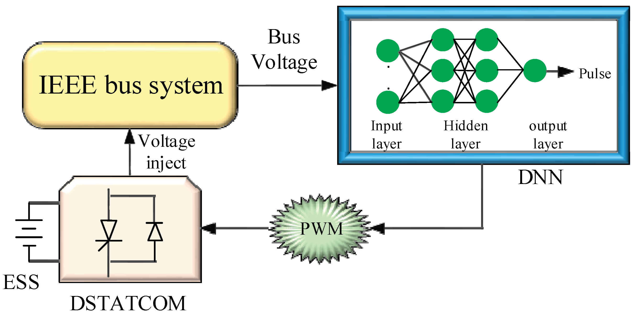
Figure 2.
Equivalent circuit of DSTATCOM.
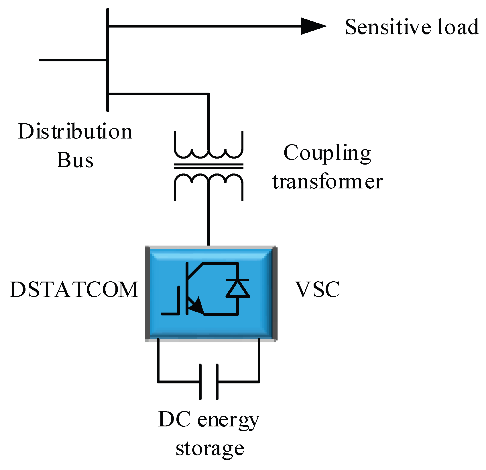
Figure 3.
Architecture model of DNN network.
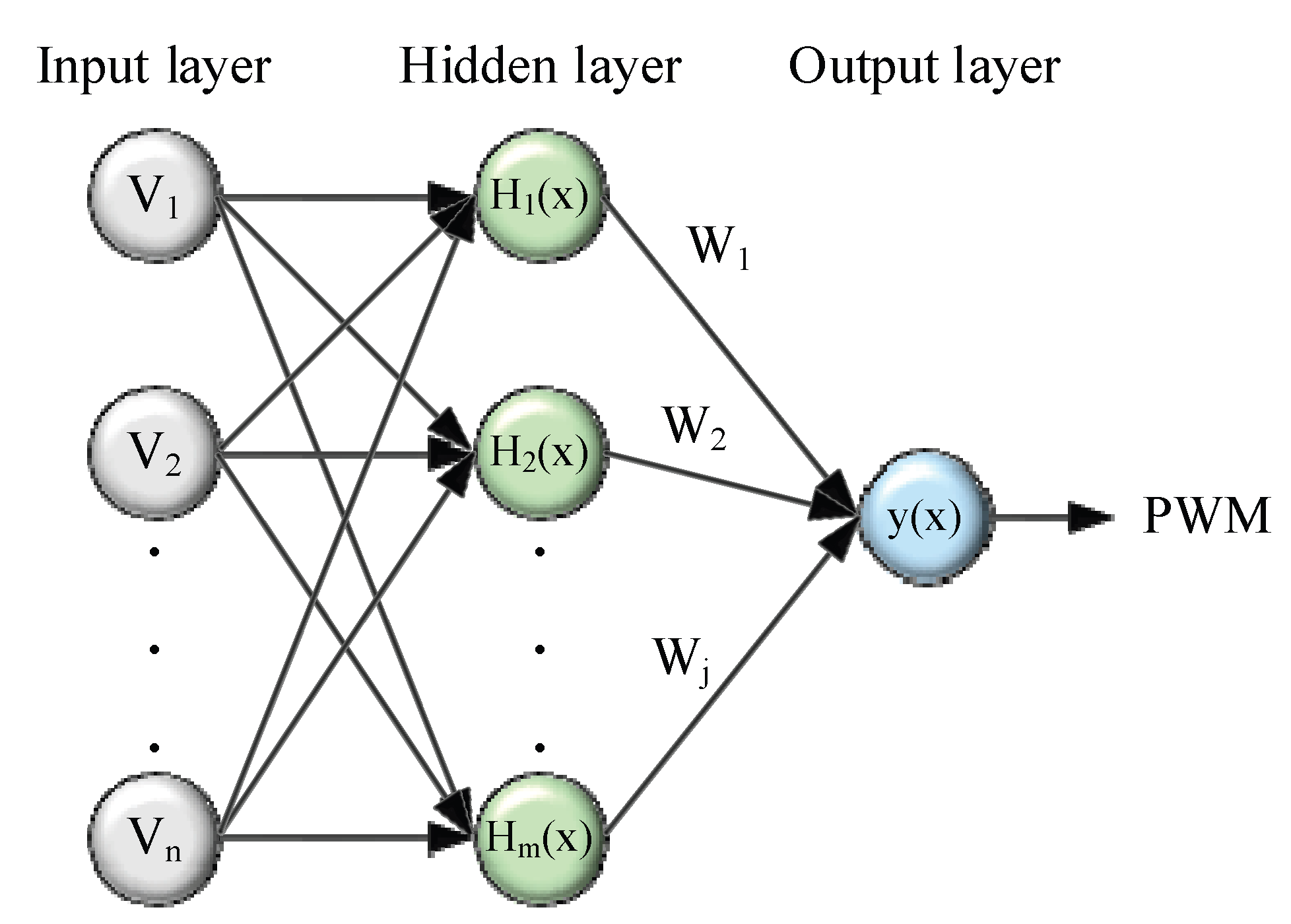
Figure 4.
Voltage waveforms of (a) Source (b) injected (c) load at sag period.
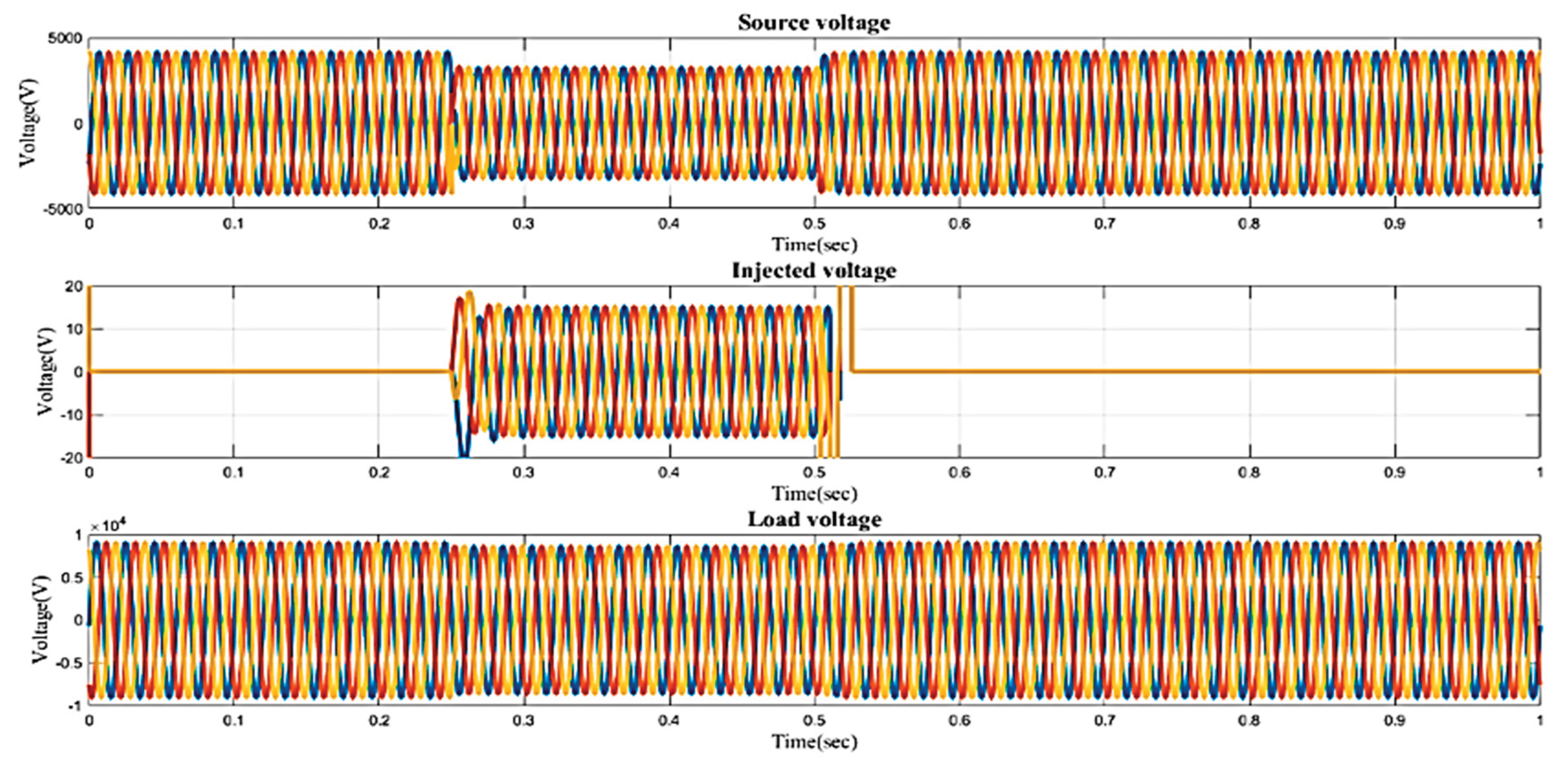
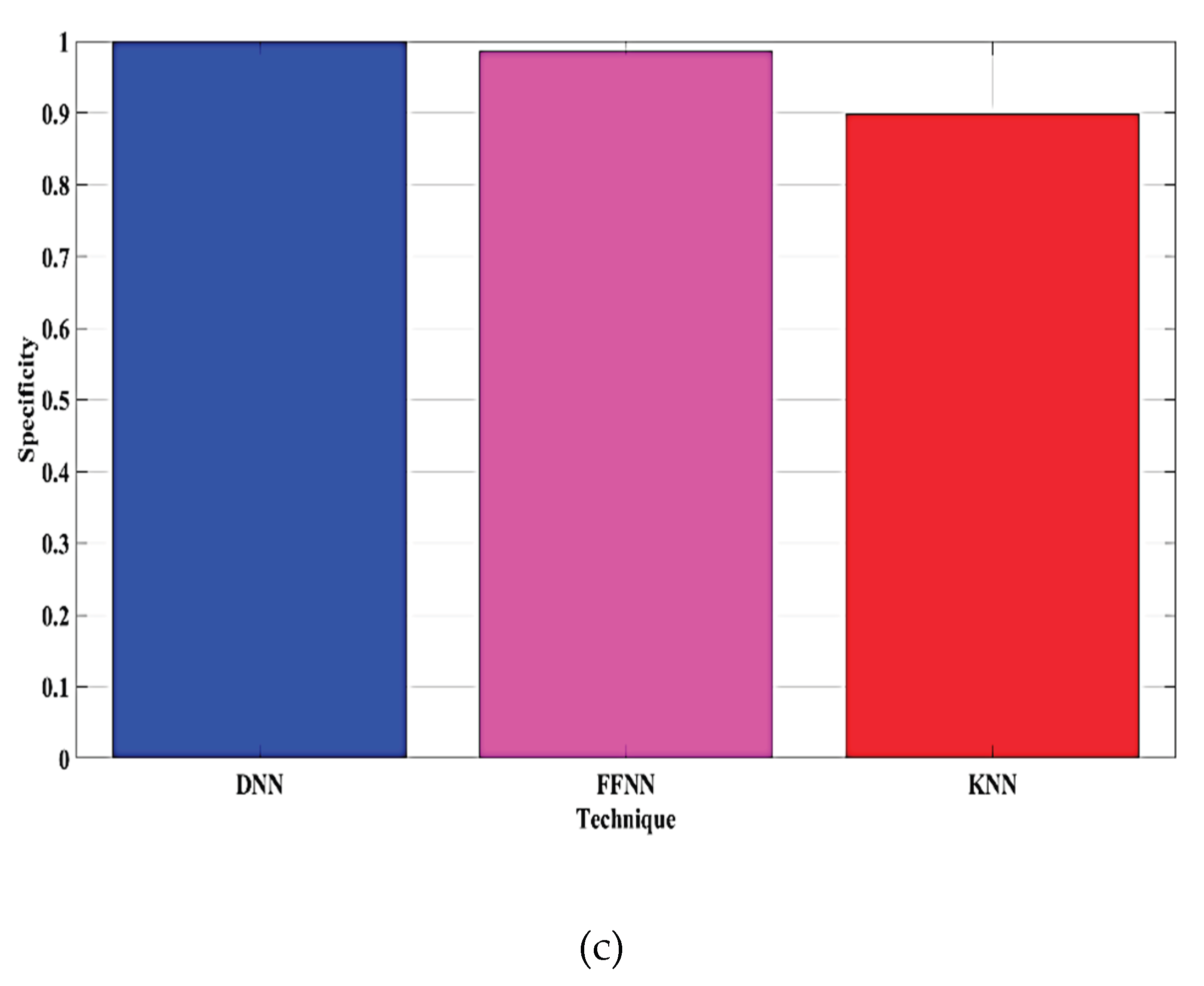
Figure 5.
Load voltage THD after sag compensation.
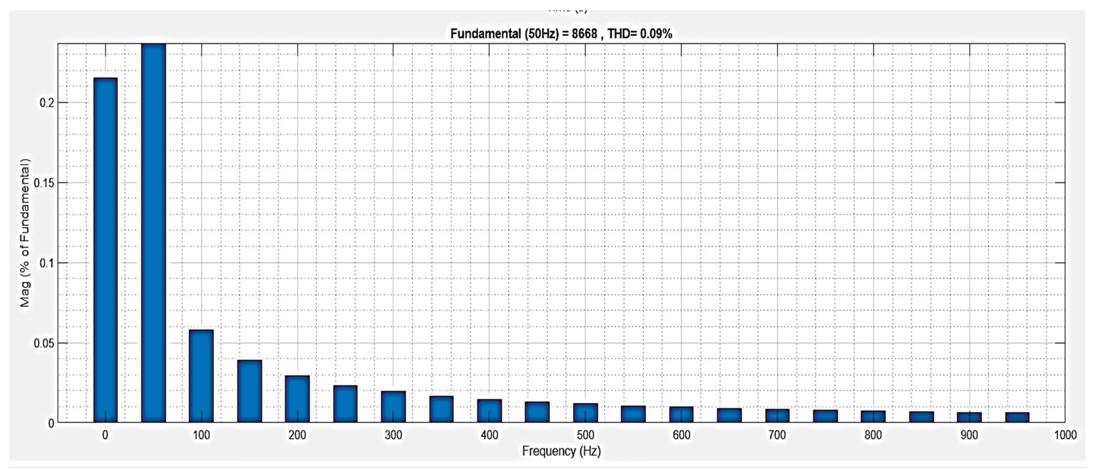
Figure 6.
Voltage waveforms of (a) source (b) inject (c) load at swell period.
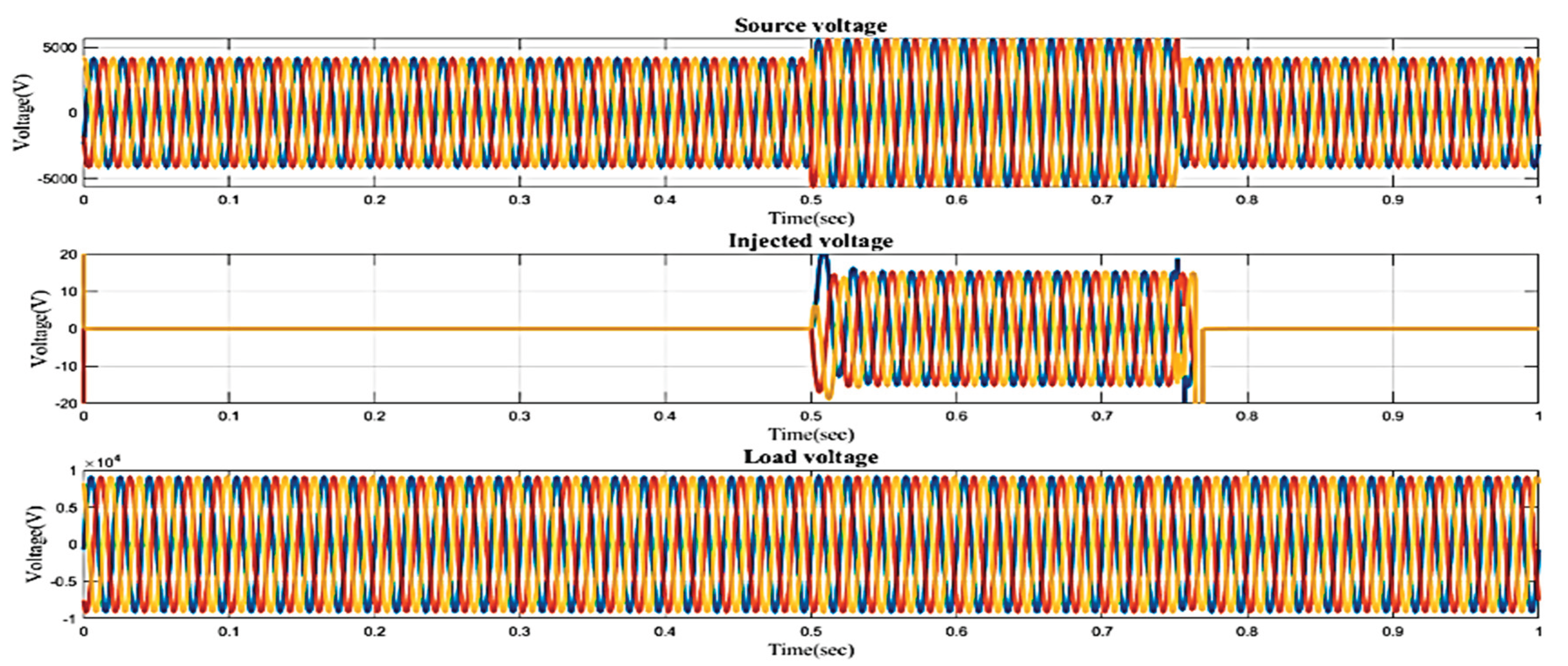
Figure 7.
Load voltage THD after swell compensation.
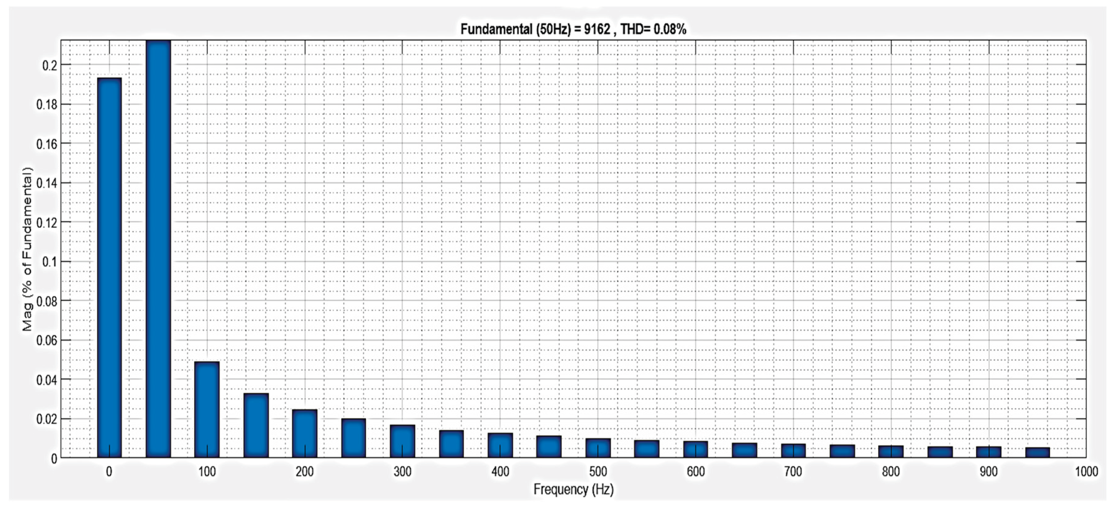
Figure 8.
Voltage waveforms of (a) source (b) inject (c) load at interruption period.
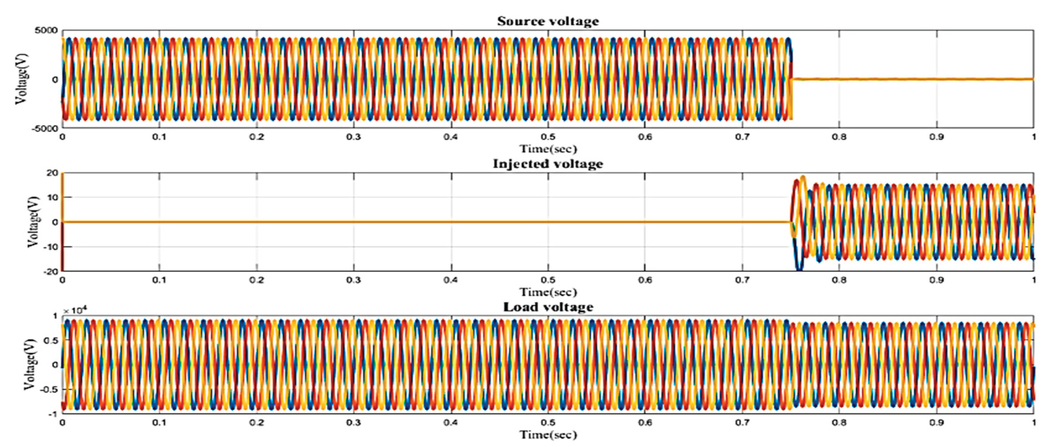
Figure 9.
Load voltage THD after interruption compensation.
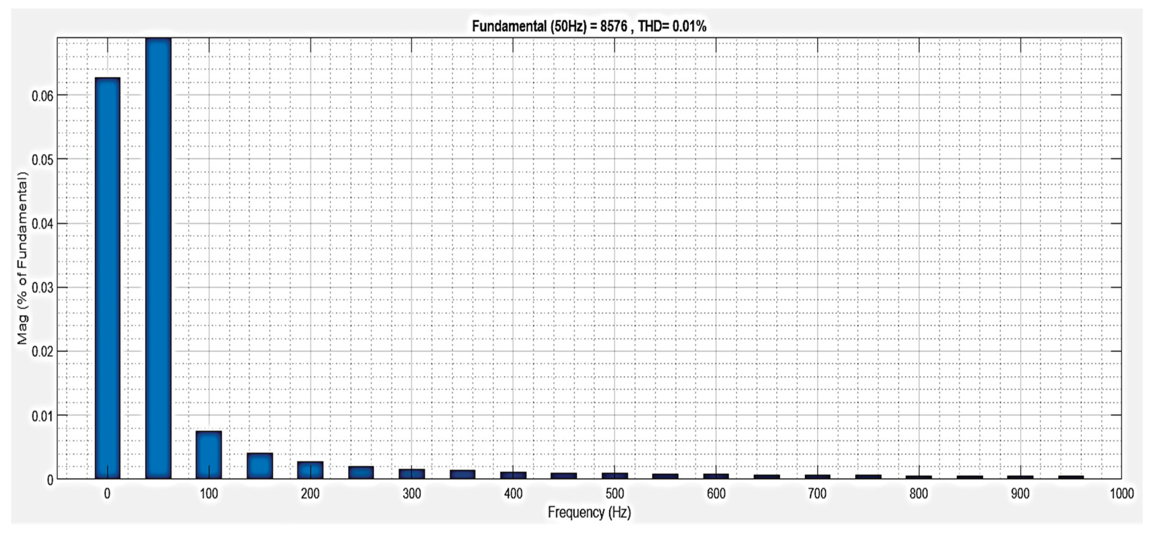
Figure 10.
Comparison of (a) Accuracy (b) Error (c) F1_score.
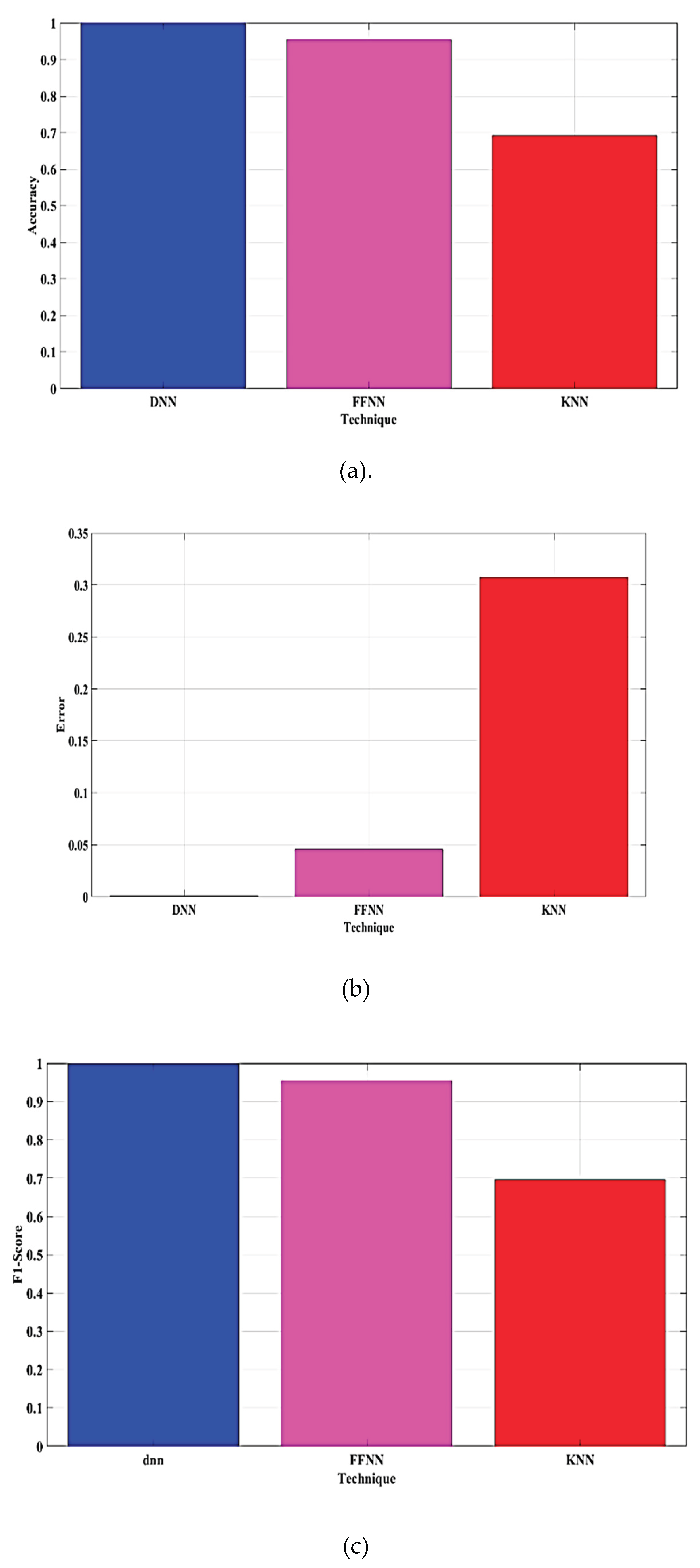
Figure 11.
Comparison of (a) FPR (b) Kappa (c) MCC.
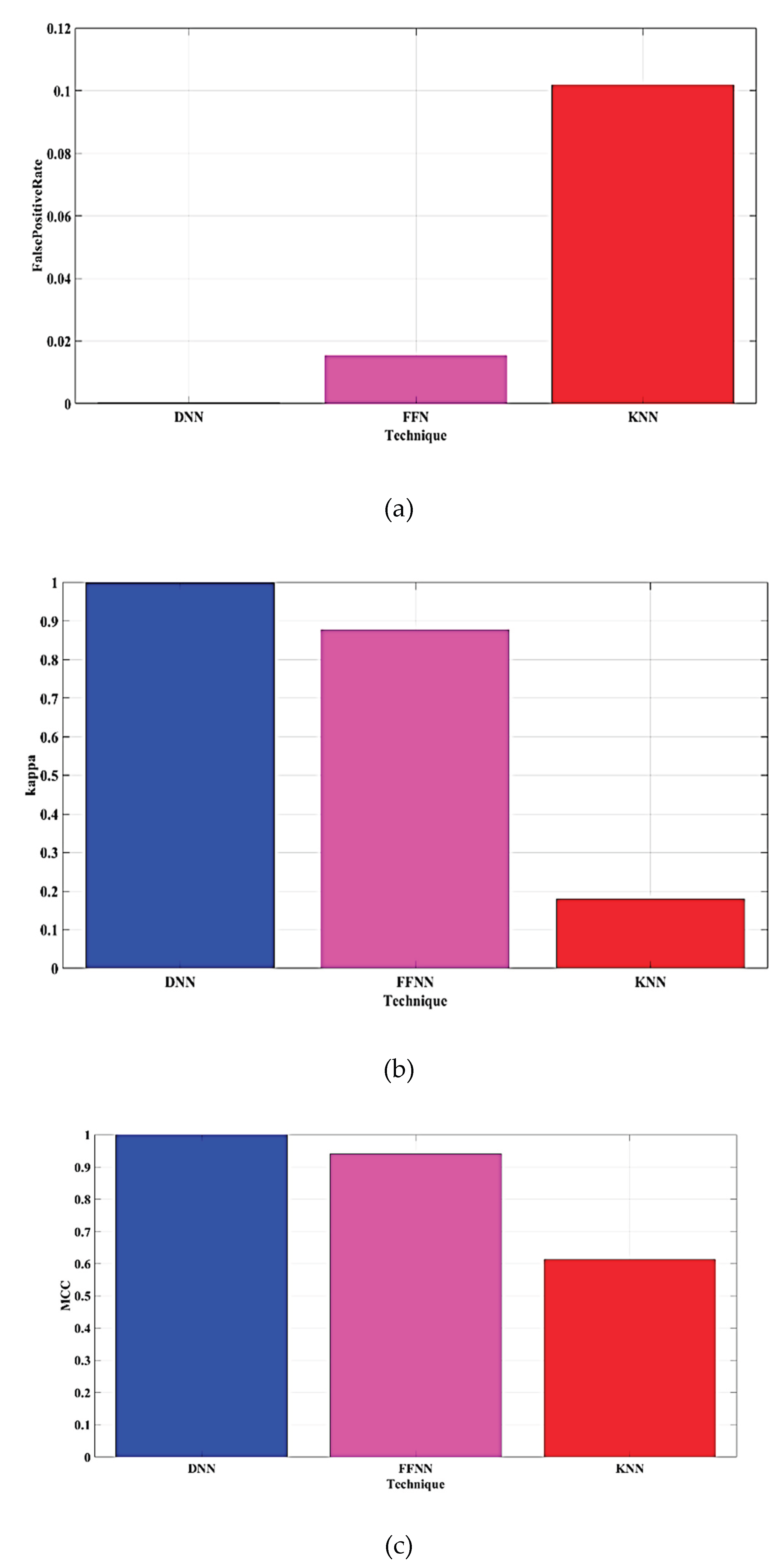
Figure 12.
Comparison of (a) Precision (b) Sensitivity (c) Specificity.
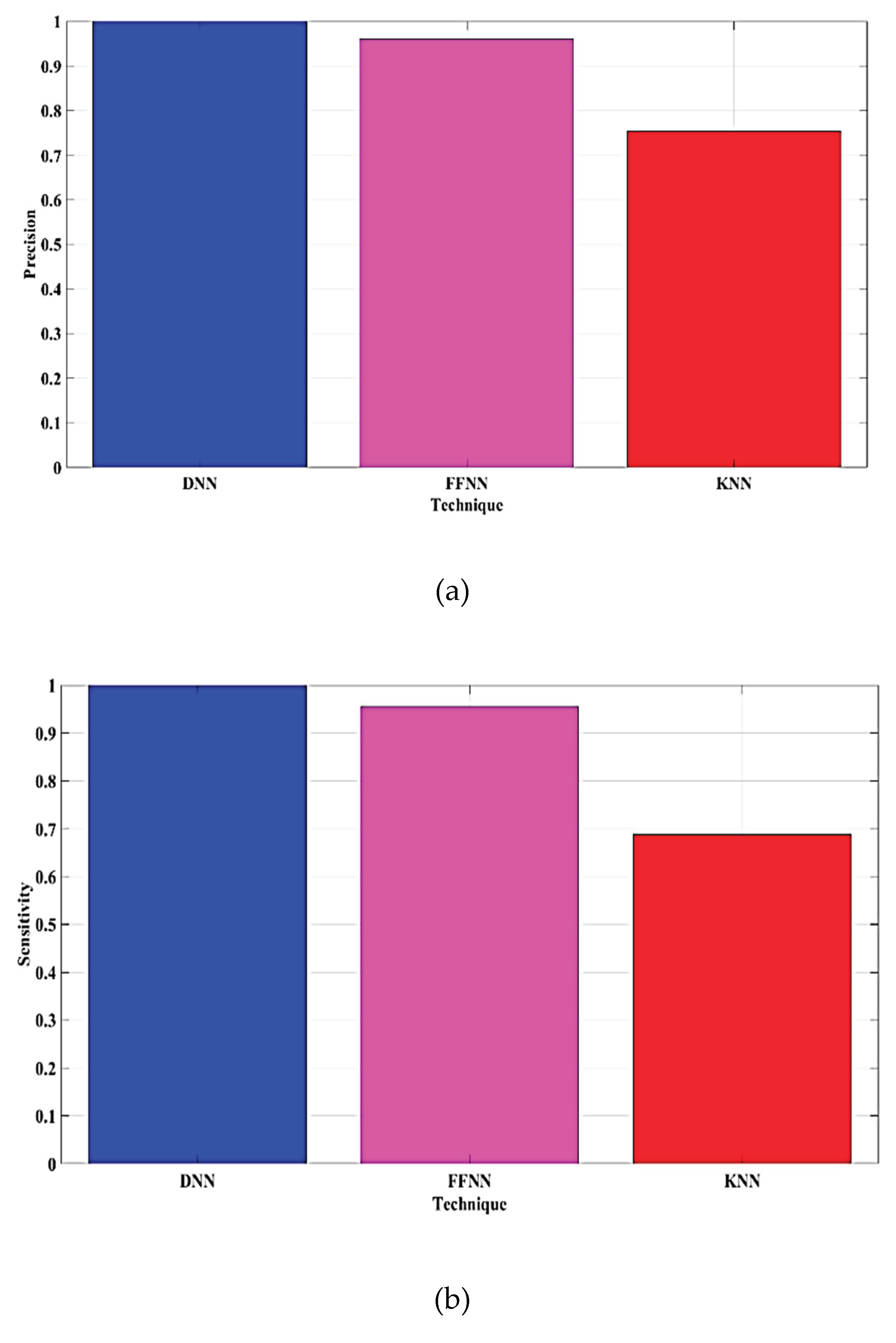
Figure 13.
Voltage waveforms of (a) Source (b) injected (c) load at sag period.
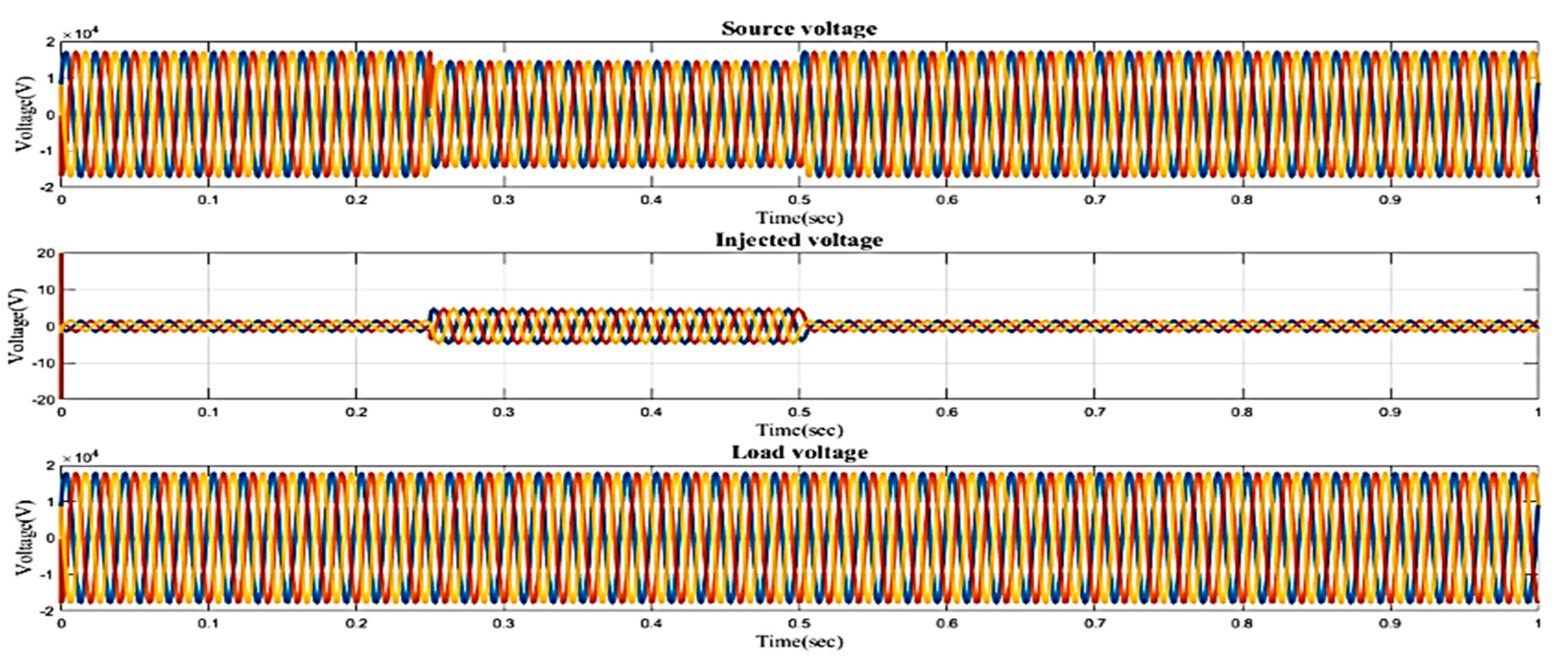
Figure 14.
Load voltage THD after sag compensation.
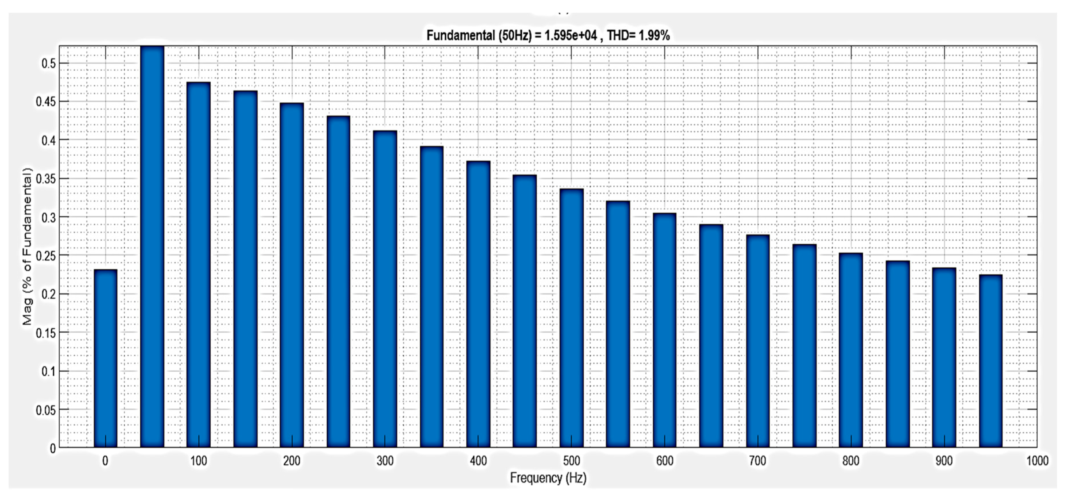
Figure 15.
Voltage waveforms of (a) source (b) inject (c) load at swell period.
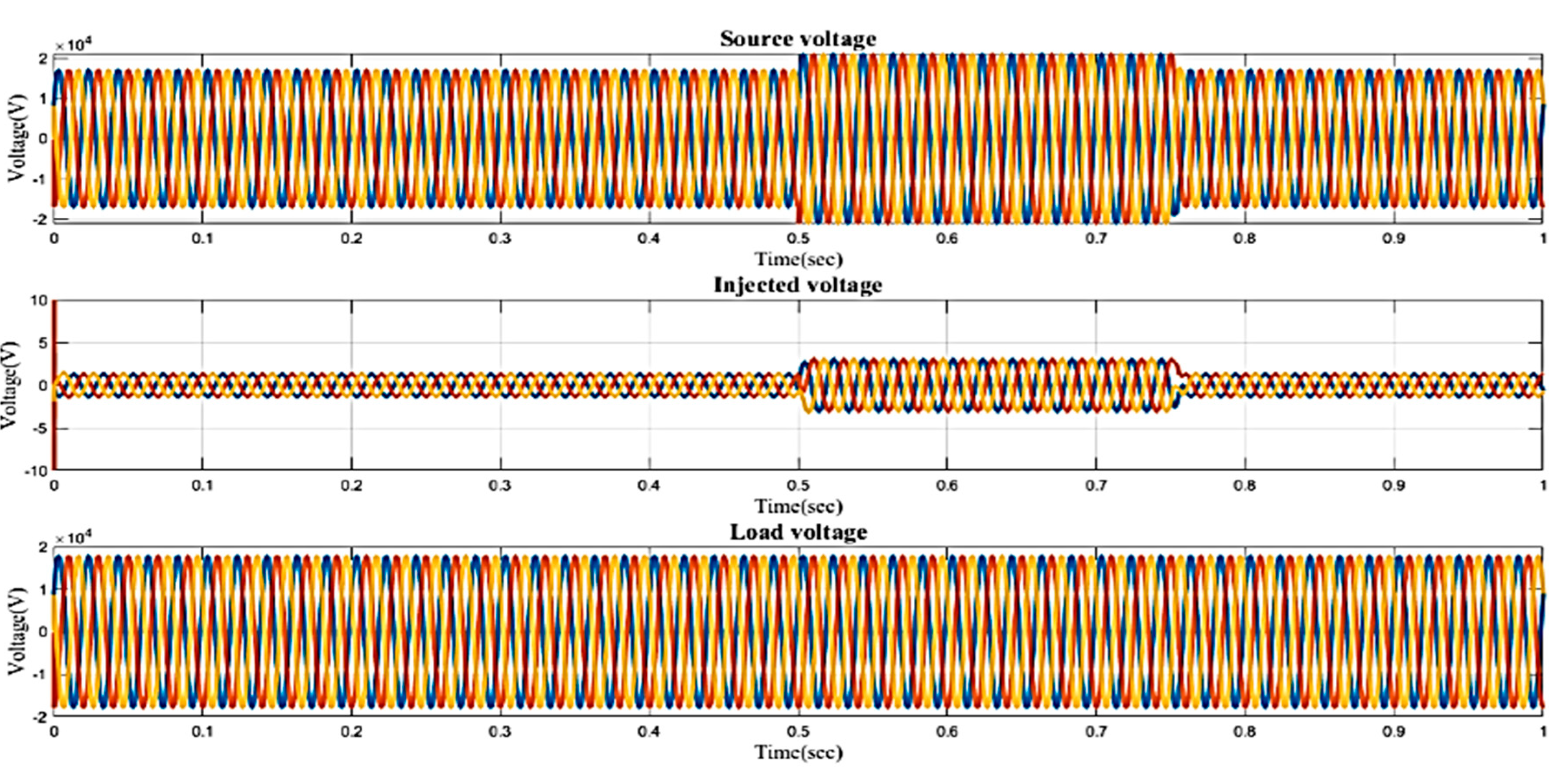
Figure 16.
Load voltage THD after swell compensation.
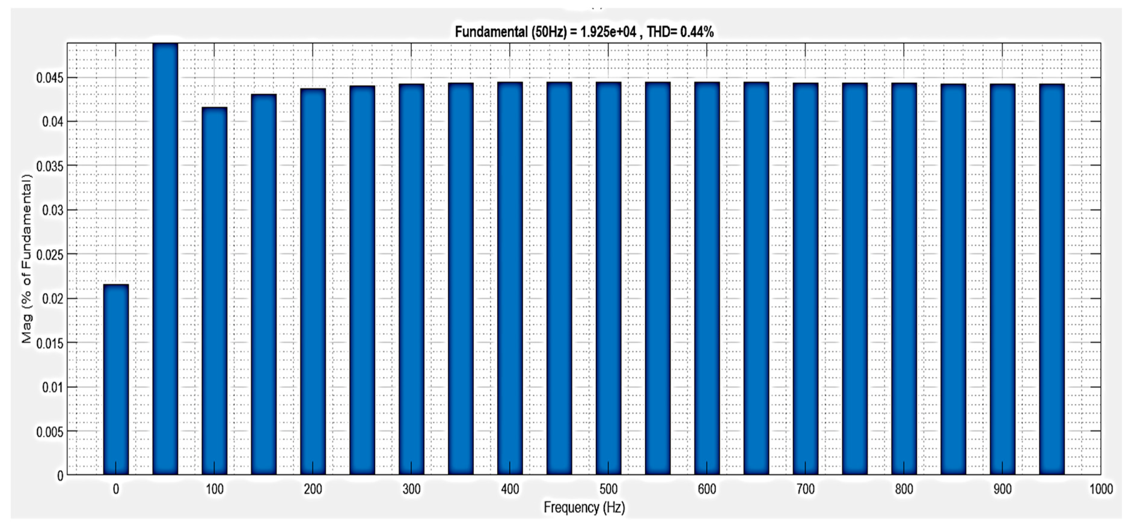
Figure 17.
Voltage waveforms of (a) source (b) inject (c) load at interruption period.
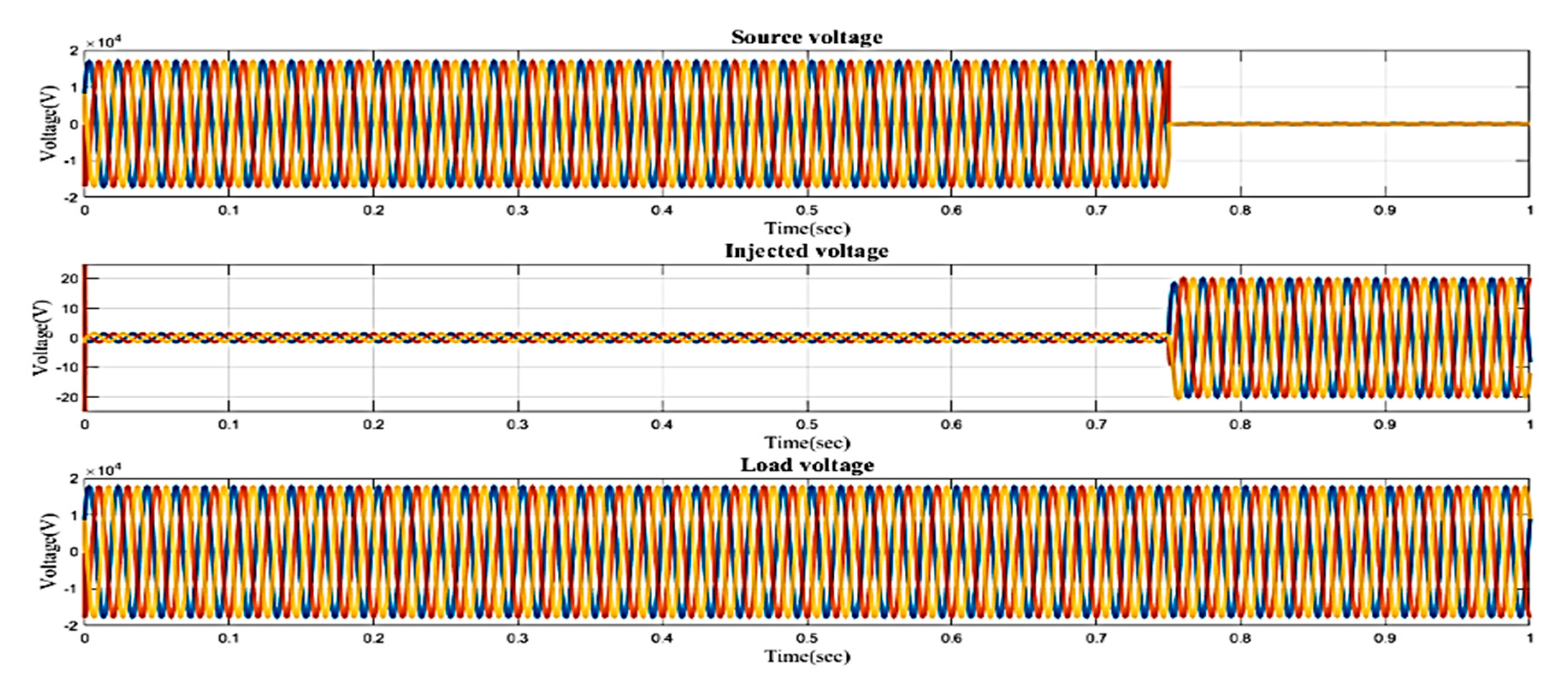
Figure 18.
Load voltage THD after interruption compensation.
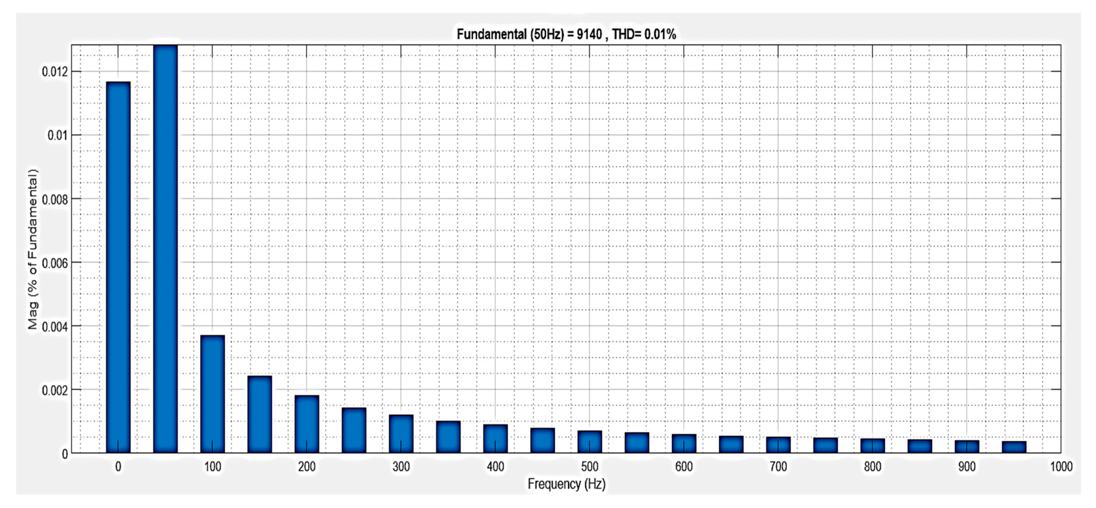
Figure 19.
Comparison of (a) Accuracy (b) Error (c) F1_score.
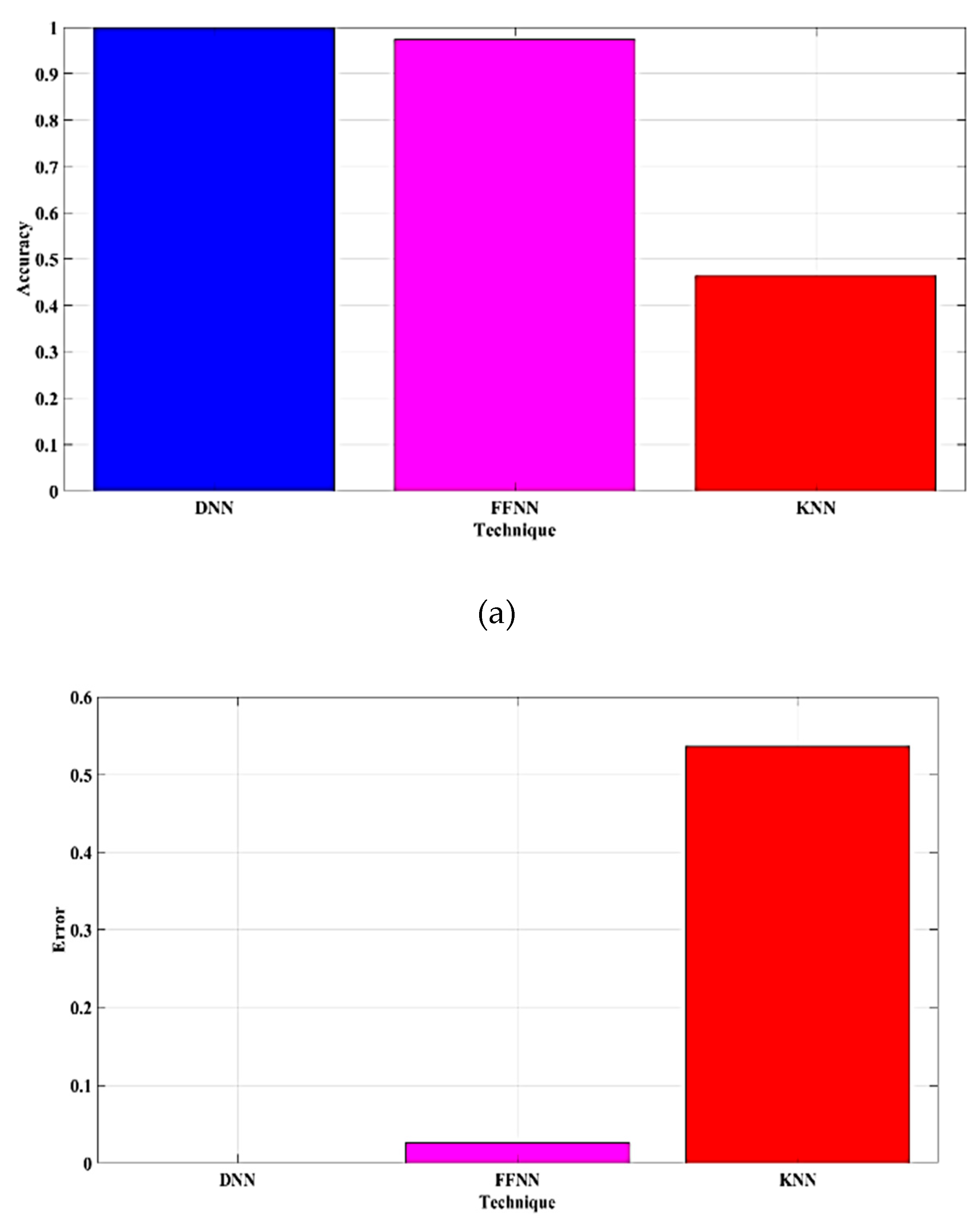
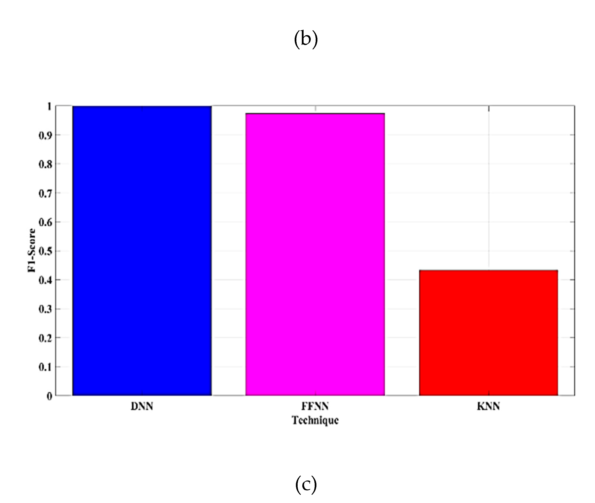
Figure 20.
Comparison of (a) FPR (b) kappa (c) MCC.
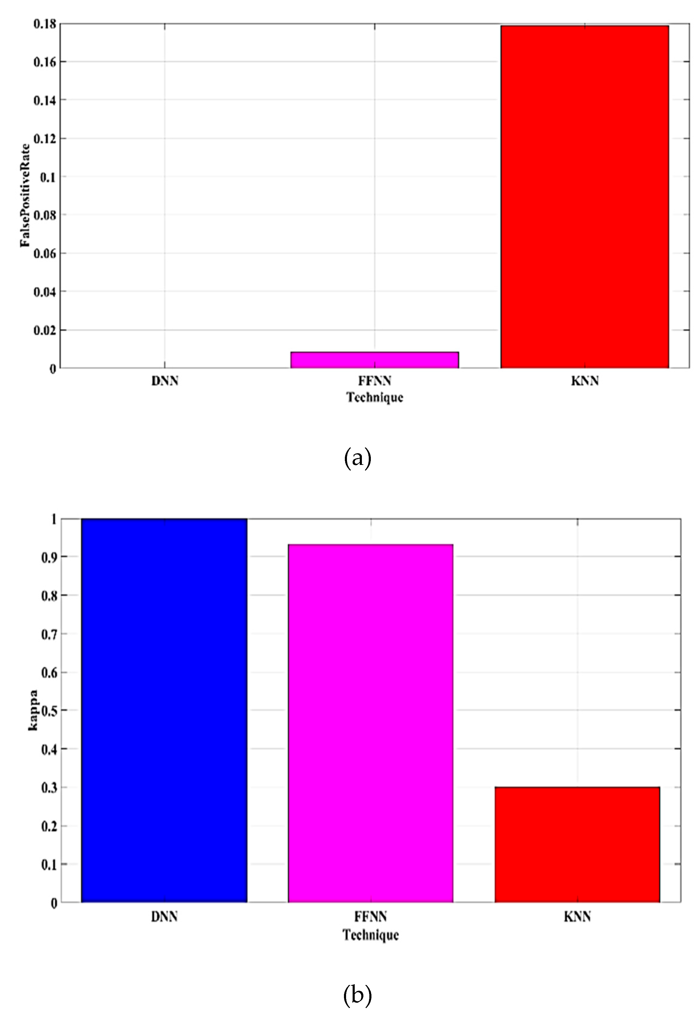
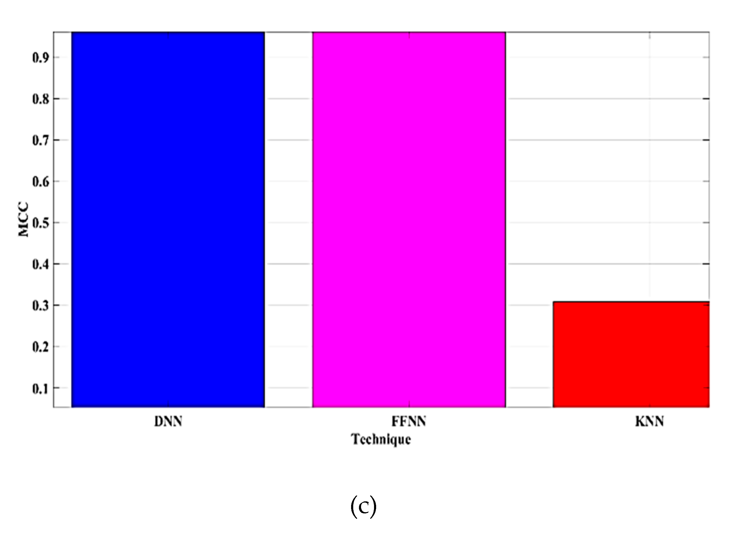
Figure 21.
Comparison of (a) Precision (b) Sensitivity (c) Specificity.
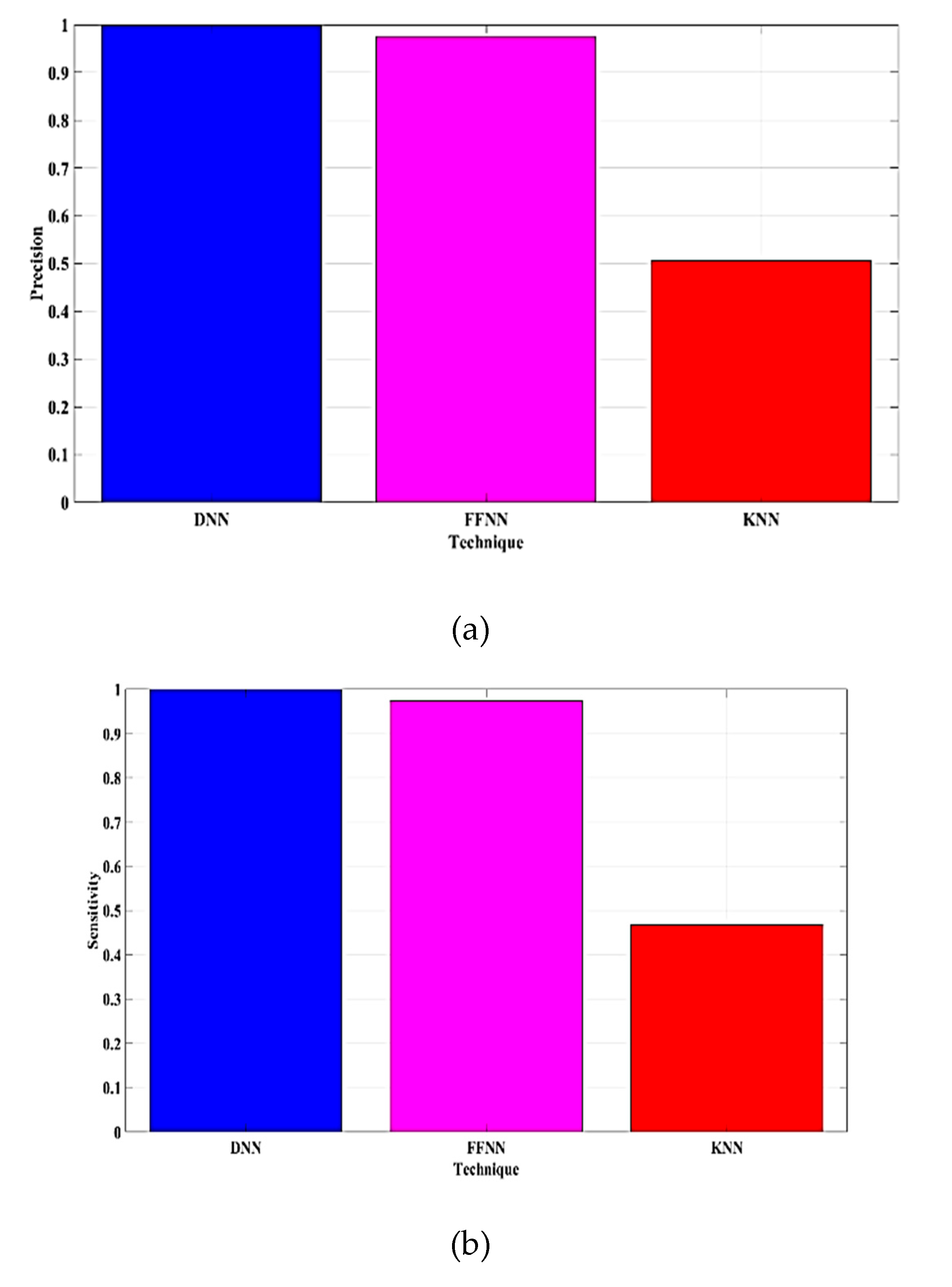
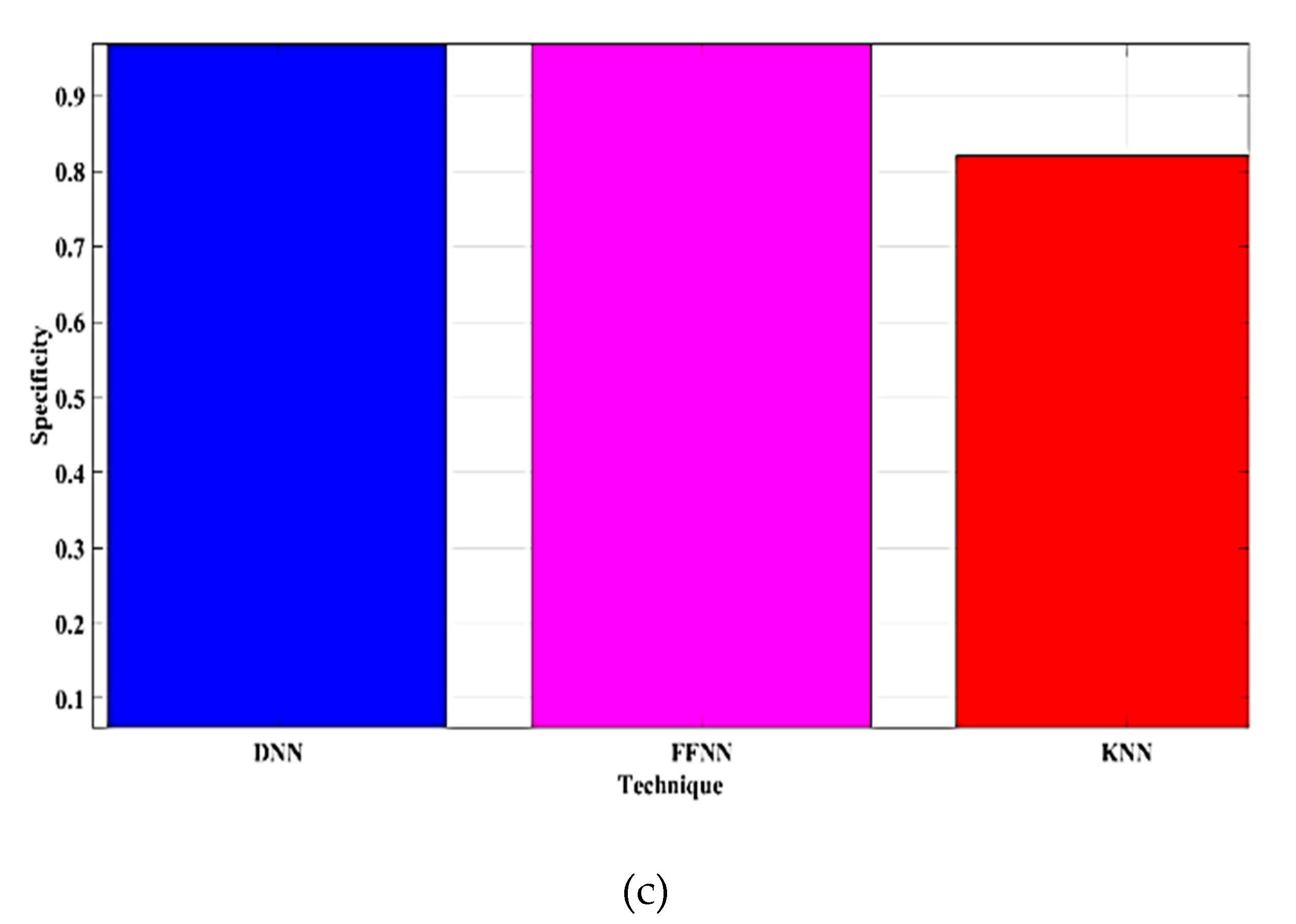

Table 1.
STATCOM parameter.
| Parameter | Ranges |
|---|---|
| Capacitance | 1000 e-6 F |
| Initial voltage | 800V |
Table 2.
Simulation parameters of proposed and existing approaches.
| Parameter | Method | Ranges |
|---|---|---|
| Hidden neuron | DNN | 10 |
| Epoch | 30 | |
| Epoch | FFNN |
100 |
| Gradient | 6.8e-05 | |
| µ | 1e-07 | |
| Training algorithm | Levenberg-Marquardt | |
| Num. Neighbors | KNN | 5 |
| Num. Observations | 150 | |
| Distance | Euclidean |
Table 3.
Dataset samples.
| Dataset | IEEE 13 bus | IEEE 33 bus |
|---|---|---|
| Overall data | 20000 | 20000 |
| Attributes | 39 | 99 |
Table 4.
Load flow analysis of IEEE 13 bus system.
| Bus no. | Voltage (V) | Sag (V) |
Swell (V) |
Interruption (V) |
|---|---|---|---|---|
| 1 | 3417 | 2890 | 3900 | 2300 |
| 2 | 4100 | 3560 | 4630 | 3325 |
| 3 | 4180 | 3455 | 4850 | 2200 |
| 4 | 4180 | 3278 | 5600 | 15 |
| 5 | 4180 | 2280 | 5600 | 15 |
| 6 | 10890 | 10550 | 10600 | 10500 |
| 7 | 9143 | 8677 | 9150 | 8580 |
| 8 | 6937 | 6340 | 7300 | 6000 |
| 9 | 7175 | 6800 | 7450 | 6665 |
| 10 | 6860 | 6445 | 7150 | 6265 |
| 11 | 6650 | 6200 | 6950 | 6000 |
| 12 | 6600 | 6125 | 6920 | 5858 |
| 13 | 6770 | 6230 | 7105 | 6910 |
Table 5.
Load flow analysis of IEEE 33 bus system.
| Bus no. | Voltage (V) | Sag (V) | Swell (V) | Interruption (V) |
|---|---|---|---|---|
| 1 | 1.79*104 | 1.7885*104 | 1.7913*104 | 1.7837*104 |
| 2 | 1.785*104 | 1.77*104 | 1.8*104 | 1.7*104 |
| 3 | 1.765*104 | 1.69*104 | 1.865*104 | 1.334*104 |
| 4 | 1.7578*104 | 1.67*104 | 1.874*104 | 1.25*104 |
| 5 | 1.75*104 | 1.65*104 | 1.88*104 | 1.175*104 |
| 6 | 1.736*104 | 1.6*104 | 1.915*104 | 9680 |
| 7 | 1.734*104 | 1.6*104 | 1.9*104 | 1*104 |
| 8 | 1.732*104 | 1.618*104 | 1.894*104 | 1*104 |
| 9 | 1.725*104 | 1.607*104 | 1.89*104 | 1*104 |
| 10 | 1.724*104 | 1.61*104 | 1.888*104 | 1*104 |
| 11 | 1.725*104 | 1.61*104 | 1.883*104 | 1*104 |
| 12 | 1.725*104 | 1.6*104 | 1.887*104 | 1*104 |
| 13 | 1.718*104 | 1.58*104 | 1.9*104 | 9400 |
| 14 | 1.7162*104 | 1.58*104 | 1.9*104 | 9050 |
| 15 | 1.715*104 | 1.58*104 | 1.91*104 | 8700 |
| 16 | 1.712*104 | 1.564*104 | 1.92*104 | 8000 |
| 17 | 1.705*104 | 1.5*104 | 1.95*104 | 6200 |
| 18 | 1.703*104 | 1.5*104 | 1.97*104 | 5450 |
| 19 | 1.781*104 | 1.76*104 | 1.80*104 | 1.667*104 |
| 20 | 1.754*104 | 1.688*104 | 1.84*104 | 1.37*104 |
| 21 | 1.7468*104 | 1.668*104 | 1.856*104 | 1.275*104 |
| 22 | 1.74*104 | 1.65*104 | 1.864*104 | 12000 |
| 23 | 1.752*104 | 1.642*104 | 1.9*104 | 1750 |
| 24 | 1.734*104 | 1.55*104 | 2*104 | 5400 |
| 25 | 1.72*104 | 1.456*104 | 2.1*104 | 78 |
| 26 | 1.734*104 | 1.6*104 | 1.82*104 | 9130 |
| 27 | 1.731*104 | 1.584*104 | 1.94*104 | 8357 |
| 28 | 1.722*104 | 1.5*104 | 2*104 | 5000 |
| 29 | 1.715*104 | 1.5*104 | 2.07*104 | 2300 |
| 30 | 1.700*104 | 1.5*104 | 2.02*104 | 2785 |
| 31 | 1.703*104 | 1.5*104 | 2*104 | 3750 |
| 32 | 1.7*104 | 1.5*104 | 2*104 | 4300 |
| 33 | 1.7*104 | 1.5*104 | 2*104 | 5000 |
Table 6.
Performance metrics comparison.
| Metrics | IEEE 13 bus system | IEEE 33 bus system |
|---|---|---|
| Accuracy | 99.9 | 99.9 |
| Error | 0.1 | 0.1 |
| F1_score | 99.9 | 99.9 |
| False positive rate | 0.01 | 0.01 |
| Kappa | 99.9 | 99.9 |
| MCC | 99.9 | 99.9 |
| Precision | 99.9 | 99.9 |
| Sensitivity | 99.9 | 99.9 |
| Specificity | 99.9 | 99.9 |
Table 7.
THD comparison.
| Condition | IEEE 13 bus system THD | IEEE 33 bus system THD |
|---|---|---|
| Sag | 0.09 | 1.99 |
| Swell | 0.08 | 0.44 |
| Interruption | 0.01 | 0.01 |
Table 8.
Comparison of THD at sag condition.
| Parameters | A-LMS [26] |
VSC [27] |
Deep Reinforcement Learning(IC-DSTATCOM)[28] |
Proposed FFNN | |
|---|---|---|---|---|---|
| IEEE 13 bus | IEEE 33 bus | ||||
| Load side THD | 1.21% | 3.65% | 27.90%% | 0.09% | 1.99% |
| Source side THD | - | 21.10% | 0.94% | 0% | 0% |
Table 9.
Ablation study for the model.
| Model Variation | No.of Hidden Layers | Neurons Per Layer | Total Weights | THD(%)IEEE 13-Bus(Sag) | THD(%)IEEE 33-Bus(Sag) |
|---|---|---|---|---|---|
| Baseline(proposed) | 1 | 10 | 1100 | 0.09 | 1.99 |
| Variation 1 | 2 | 20 | 4200 | 0.07 | 1.50 |
| Variation 2 | 3 | 30 | 9300 | 0.05 | 1.20 |
| Variation 3 | 4 | 50 | 20500 | 0.04 | 1.10 |
| Variation 4 | 2 | 10 | 2200 | 0.08 | 1.70 |
Table 10.
Scenario Based Performances of Proposed Model.
| Scenario No | Power Load(kw) | Harmonic Distortion(%) | Control Unit Location | THD After Compensation(%) |
|---|---|---|---|---|
| 1 | 500 | 5 | Bus 5 | 0.09 |
| 2 | 750 | 7 | Bus 5 | 0.12 |
| 3 | 500 | 10 | Bus 10 | 1.12 |
| 4 | 1000 | 5 | Bus 15 | 0.18 |
| 5 | 600 | 8 | Bus 5 | 0.11 |
| 6 | 750 | 12 | Bus 10 | 1.20 |
Disclaimer/Publisher’s Note: The statements, opinions and data contained in all publications are solely those of the individual author(s) and contributor(s) and not of MDPI and/or the editor(s). MDPI and/or the editor(s) disclaim responsibility for any injury to people or property resulting from any ideas, methods, instructions or products referred to in the content. |
© 2025 by the authors. Licensee MDPI, Basel, Switzerland. This article is an open access article distributed under the terms and conditions of the Creative Commons Attribution (CC BY) license (http://creativecommons.org/licenses/by/4.0/).
Copyright: This open access article is published under a Creative Commons CC BY 4.0 license, which permit the free download, distribution, and reuse, provided that the author and preprint are cited in any reuse.


