
Submitted:
16 September 2025
Posted:
26 September 2025
You are already at the latest version
Abstract
The operational modes and fault characteristics of distribution networks incorporating distributed generation are becoming increasingly complex. This complexity increases the difficulty of predicting switch control action times, leads to scattered samples and data scarcity, and imposes higher demands on rapid fault isolation and load transfer control following system failures. To address this issue, this paper proposes a switch action time prediction and synchronous load transfer control method based on Bayesian optimization of bidirectional long short-term memory networks (Bo-BiLSTM). A distribution network simulation model incorporating distributed generation was constructed using MATLAB/Simulink. Three-phase voltage and current at the point of common coupling (PCC) were extracted as feature parameters to establish a switch operation timing database. Bayesian optimization was employed to tune the BiLSTM hyperparameters, constructing the Bo-BiLSTM prediction model to achieve high-precision forecasting of switch operation times under fault conditions. Subsequently, a load-synchronized transfer control strategy was proposed based on the prediction results. A dynamic delay mechanism was designed to achieve “disconnect-first, reconnect-later” sequential coordinated control. Physical experiments verified that the time difference between disconnection and reconnection was controlled within 2–12 ms, meeting the engineering requirement of less than 20 ms. Results demonstrate that the proposed control method enhances switch operation time prediction accuracy while effectively supporting rapid fault isolation and seamless load transfer in distribution networks, thereby improving system reliability and control precision.
Keywords:
distributed power sources
; Bayesian optimization
; switching action time
; time prediction
; load synchronous transfer control
1. Introduction
With the large-scale integration of distributed generation (DG) into distribution networks, system operation modes and fault characteristics have become increasingly complex, placing higher demands on rapid fault isolation and load transfer control post-fault [1]. As the core component enabling distribution network automation and fault self-healing, the precise prediction of switching equipment response times is crucial for ensuring reliable operation of protection and control systems and minimizing outage duration [2]. However, DG integration significantly alters fault current magnitude and direction, resulting in highly dispersed and uncertain switch operation time samples. Concurrently, the scarcity of training data for predictive models is exacerbated by the challenges in collecting real-world fault data. These factors cause a significant decline in the accuracy of prediction methods based on traditional mechanism models or shallow learning algorithms, making it difficult to meet the stringent requirements for real-time control and reliability in smart distribution grids.
In recent years, deep learning techniques have achieved remarkable success in the field of time-series data forecasting. Long Short-Term Memory (LSTM) networks and their variants have been widely applied in areas such as equipment remaining life prediction [3,4] and power load forecasting due to their exceptional ability to capture long-term sequential dependencies. However, standard LSTM models suffer from blindness in hyperparameter selection and predominantly employ unidirectional encoding, making it difficult to fully exploit the bidirectional contextual information inherent in time-series data. Although Bidirectional LSTMs (BiLSTMs) enhance feature extraction through bidirectional encoding, their performance remains heavily dependent on optimized hyperparameter configurations [5]. Bayesian Optimization (BO), as an efficient global hyperparameter optimization framework, can adaptively search for optimal hyperparameter combinations of complex models with minimal evaluation iterations, significantly improving model convergence speed and prediction accuracy [6]. To date, no research has reported the deep integration of BO with BiLSTM (Bo-BiLSTM) for application in distribution network switch timing prediction and cooperative control [7,8].
Based on this, this paper addresses the challenge of high-precision prediction of switch operation times in distribution networks under DG integration, and further applies the prediction results to the precise control of load synchronous transfer. The main contributions of this study are as follows:
- A Bo-BiLSTM-based prediction model for switching operation timing in distribution networks is proposed. By adaptively obtaining optimal hyperparameters for the BiLSTM network through Bayesian optimization algorithms, the model’s predictive accuracy and generalization capability are effectively enhanced under conditions of small sample sizes and high data dispersion, laying the foundation for subsequent implementation of control strategies.
- A comprehensive database of switch operation time characteristics has been established. A detailed simulation model of the distribution network incorporating distributed generation (DG) was constructed using MATLAB/Simulink. This model simulated 310 operational scenarios encompassing various short-circuit fault types, different fault locations, and transition resistances, providing a robust data foundation for model training and control logic validation.
- Innovatively integrating switch timing prediction results with load transfer control strategies. Based on the predicted time parameters, a synchronous transfer control strategy was designed following the principle of “disconnect first, then connect,” with dynamic delay Δt as its core. Physical experiments validated that this strategy can strictly control the disconnect-connect time difference within the 20 ms safety margin, with experimental results ranging from 2 to 12 ms. This fundamentally eliminates the risk of circulating currents caused by asynchronous closing, achieving seamless load transfer control after a fault.
This study not only provides a novel data-driven solution for predicting the switching control action time in distribution networks but also establishes a comprehensive technical framework spanning from “precise prediction” to “precise control.” It holds significant theoretical value and engineering significance for enhancing the power supply reliability and self-healing control capabilities of distribution networks under high-penetration distributed generation (DG) access.
2. Simulation Modeling and Feature Database Construction
2.1. Simulation Modeling
This paper is based on the typical structure of distribution networks and distributed photovoltaic systems, as illustrated in Figure 1.
Typical distributed power sources in distribution networks are connected to the 10kV distribution grid via DYn11 transformers. The main system equipment and model parameters are listed in Table 1.
A distribution network simulation model was established using MATLAB/Simulink. Simulations were conducted to analyze the distribution network conditions when different types of faults occurred at various locations (f1, f2, f3) of the distributed power sources. Subsequently, the switching operation times of the distribution network switches were recorded and analyzed from both voltage and current perspectives after the distributed power sources were connected to the distribution network. This provides historical data support for subsequent predictive control.
2.2. Construction of a Database for Time Characteristics of Distribution Network Switch Operations
Point of Common Coupling (PCC) refers to a common point or location within a power system where multiple customers and their equipment connect to the public grid. Real-time monitoring and analysis of parameters such as current, voltage, frequency, harmonics, and interruptions at the PCC enables timely detection and resolution of various faults occurring in the distribution system, ensuring reliable power supply. The operational status of the grid and the type of fault will determine the switching action time [9]. Grid faults significantly impact both voltage and current at PCC points, potentially causing voltage sags, voltage dips, voltage asymmetry, and increased short-circuit currents. The magnitude of voltage sags and current surges directly determines the initiation criteria and action sequence of protective devices. Therefore, this paper selects the three-phase voltage and three-phase current at the PCC as predictive parameters for switch control action timing, establishing a database of distribution network switch action characteristics.

Table 2.
Time-Characteristic Parameters of Grid Switch Operation.
| Variables | parameter |
|---|---|
| VA | Phase A voltage peak |
| VB | Phase B voltage peak |
| VC | Phase C voltage peak |
| IA | Phase A current peak |
| IB | Phase B current peak |
| IC | Phase C current peak |
| T | Switching Time |
Distribution networks can be broadly categorized into 12 operational conditions: single-phase short circuits (AG, BG, CG), two-phase short circuits (AB, AC, BC), two-phase grounded short circuits (ABG, ACG, BCG), three-phase short circuit (ABC), three-phase short circuit to ground (ABCG), and non-fault state [10]. Simulations were conducted for different distribution network operating conditions, collecting three-phase voltages and currents at the PCC for each condition to construct a database of switch operating time characteristics for distribution networks. A total of 310 operating conditions were obtained, denoted as O1-O310. The six characteristic data sets and switch operation times for different operating conditions are shown in Table 3.
To eliminate the effects of different dimensions, it is necessary to normalize the eigenmatrix. Using the discrete normalization method, the eigenvalues of O1 to O310 can be transformed into the effective range [0,1]. Taking O1 as an example, the normalization process follows the method described in [11]:
In the formula, Vi and Vi’ denote the normalized and pre-normalized values of the i-th operational state symptom attribute, respectively; Vmax and Vmin represent the maximum and minimum values of Vi. Similarly, calculate S2 through S310. The normalized database is shown in Table 4.
The normalization of the feature matrix involves six operational status indicators for each operating condition in the database, collectively forming a feature vector. A training dataset comprising 310 × 70% = 217 feature vectors is randomly selected from the database, while the remaining 310 × 30% = 93 vectors serve as the test dataset.
3. Bayesian Optimization-Based BiLSTM Forecasting Model
3.1. BiLSTM Principles and Applicability
The LSTM algorithm is used to process and predict highly time-dependent, strongly coupled events, but LSTM network models exhibit lower adaptability [12]. Unlike LSTM networks, the BiLSTM consists of two independent forward and backward LSTMs, one for forward propagation and the other for backward propagation. At each time step, the forward LSTM processes the input sequence in ascending order, while the backward LSTM processes it in descending order. This allows each LSTM unit to simultaneously access both preceding and subsequent contextual information. This study employs BiLSTM to capture the temporal characteristics of electrical quantities before and after failures, performing bidirectional training on sample failure data. The schematic diagram of the BiLSTM structure is shown in Figure 2.
3.2. Bayesian Optimization Principle
Bayesian optimization employs Gaussian processes as probabilistic surrogate models, enhancing algorithmic robustness through continuous iteration on existing sample data [13]. When determining new prediction points, Bayesian algorithms require maximizing the utility function. Thus, while not applicable to every optimization problem, Bayesian algorithms constitute an effective global optimization approach. Bayesian optimization comprises Gaussian process regression and acquisition function computation. Gaussian process regression yields the mean and variance of the function value, while the acquisition function constructs a sampling strategy based on these parameters to determine the sampling points for the current iteration.
(1) Gaussian Process Regression
Gaussian Process Regression (GPR) is a nonparametric Bayesian method for solving regression problems [14]. GPR is based on a Gaussian process prior distribution, which is adjusted by observational data to yield a posterior distribution [15]. Its model assumptions comprise both noise and Gaussian process prior components, with solutions derived through Bayesian inference.
(2) Collection Function
The sampling function generates the next observation point to be predicted. Based on the mean and covariance dataset D calculated by Gaussian process regression, it determines the next sample point after iteration. Its primary role is to accelerate convergence by leveraging previous observations while simultaneously exploring regions of high uncertainty within the decision space, thereby avoiding getting stuck in local optima.
3.3. Bo-BiLSTM Network Parameter Optimization
The hyperparameters of BiLSTM are difficult to set manually, so a Bayesian optimization (BO) approach is employed to automatically identify the optimal hyperparameter combination, aiming to achieve higher prediction accuracy. Given the large number of parameters in the BiLSTM network, the BO algorithm is used to optimize several key parameters within the network. This ensures the optimized parameters achieve the best possible fit with the network, enabling high-precision data prediction.
The hyperparameter selection formula for Bayesian optimization is as follows:
In the formula, f(x) denotes the optimization function; x represents the set of optimization parameters; X is the set of optimization parameter sets; x* is a set of optimization functions.
Define the Error function as the prediction error rate function for the BiLSTM model, with the formula as follows:
In the formula, N represents the total number of sample groups; R denotes the number of sample groups in N where the predicted values match the actual loss values.
The BiLSTM weight update formula is:
In the formula, α denotes the learning rate; n represents the mini-batch size. It can be seen from the formula that α and n influence the weight updates of the network, with α affecting the step size per iteration and n determining the network’s loss function.
3.4. Switch Operation Time Prediction Method for Distribution Networks Based on Bo-BiLSTM Network
The modeling and testing process of the Bo-BiLSTM network is illustrated in Figure 3. First, switch test data from distribution network simulations is acquired, smoothed, and divided into training and test sets. Next, the Bo algorithm is applied to tune hyperparameters on the training set, with the optimal settings fed back to reconstruct the BiLSTM network. Finally, predictions are made on the test set data.
The optimization process of the model can be divided into the following steps.
(1)Model initialization, define the function f (x) and the definition domain of x to be optimized in the Bayesian optimization algorithm, set the objective function and the maximum number of iterations, etc.; divide the processed failure characteristics data set into test set kernel and training set, and train the BiLSTM model.
(2)Select the BiLSTM model failure prediction error rate to get the initial observation of the Bayesian algorithm.
(3)The Gaussian process is applied to estimate the initial observation value to determine the next observation point.
(4)Select the optimal parameters according to the acquisition function until the end of the iteration.
(5)The optimal parameters obtained by the Bayesian algorithm are brought into the BiLSTM network for parameter reconstruction.
(6)The optimal parameters are brought into the BiLSTM model to predict the test set data, and the predicted results are obtained and analyzed.
4. Analysis of BiLSTM Prediction Model Results
4.1. Model Prediction Standard
The goodness-of-fit coefficient (R2), root mean square error (RMSE), and mean absolute error (MAE) can be used to evaluate the performance of time series forecasting algorithms [16]. R2 indicates the degree of fit between the data and the regression model; RMSE represents the average value of errors, reflecting the model’s stability; MAE accurately reflects the magnitude of actual prediction errors. Their expressions are as follows:
In the formula, xtri is the true value, is the average of the true value, xpri is the predicted value, N is the number of predictions.
4.2. Bayesian Optimization Search Results
The results of Bayesian optimization are shown in Figure 4. The Bayesian optimization algorithm repeatedly refines the target values through the operation of the acquisition function, seeking the global optimum of the objective function through continuous function computation. This aims to optimize the BiLSTM network and ensure more accurate prediction results. The total iteration count for the sampling function was 50. Upon reaching 50 iterations, the gap between the observed minimum target value and the estimated minimum target value gradually converged toward 0.002. Based on the sampling function results, new hyperparameter combinations were selected for evaluation, enabling the Bi-LSTM network model to achieve optimization and deliver more accurate predictions.
4.3. Distribution Network Switching Time Prediction Results
The first 70% of the distribution network switch time series is used as the training set, while the remaining 30% serves as the test set. The delay step size is set to 15, the solver is configured as “adam”, and the initial learning rate is 0.005. Training is conducted for 250 epochs with a learning rate decay factor of 0.2 and a decay cycle of 125. To prevent gradient explosion, the gradient threshold is set to 1.
The prediction results for the three network models of distribution network switching times are shown in Figure 5, Figure 6, and Figure 7, respectively.
As shown in Table 5, for the prediction metrics of the distribution network switch operation time prediction model, the Bo-BiLSTM network achieved a model fit quality (R2) of 0.90401, representing improvements of 0.28486 and 0.3569 compared to the BiLSTM and LSTM networks, respectively. The root mean square error (RMSE) is 0.59982, representing reductions of 0.595 and 0.7031 compared to the BiLSTM and LSTM networks, respectively. The mean absolute error (MAE) is 0.49864, showing decreases of 0.5364 and 0.6159 relative to the BiLSTM and LSTM networks.
To more intuitively demonstrate the superiority of the Bo-BiLSTM model in time prediction, the prediction error was calculated between the predicted and actual switch operation times for the 100th sample point in the distribution network. The prediction errors for switch operation times under different network models are shown in Table 6.
The absolute error data in the table shows that the absolute errors for the three network models are 0.76186, 1.34878, and 2.1639, respectively. The Bo-BiLSTM network exhibits the smallest absolute error in model prediction, demonstrating superior performance compared to the BiLSTM and LSTM network models.
5. Time-Based Model and Experimental Validation for Full-Process Control of Load Transfer Using Bo-BiLSTM
Accurate switch timing prediction provides the prerequisite for achieving precise load transfer control.
This chapter will design a synchronous control strategy based on the switching times (Ton, Toff) predicted by the Bo-BiLSTM model to ensure the safety and rapidity of the transfer process. The core control objective of the model is to accurately estimate the total time control interval from the issuance of the master station command to the final switching action, while ensuring compliance with the “open before close” sequence and time difference constraints even under extreme scenarios. By integrating mathematical modeling with engineering experience, we can systematically evaluate the boundary conditions of time parameters and their impact mechanisms on the overall control process, providing theoretical support for strategy design. This strategy requires, based on precise time synchronization, that the time interval from complete tripping to complete closing be within 20ms, disregarding communication time from the master station to the terminal.
5.1. Time Constraints and Problem Modeling
Control Objective: Total time (interval from trip completion to close completion) must satisfy 0 < Ttotal < 20 ms.
Known Conditions:
Closing time Ton > Trip time Toff, based on switch timing (Ton, Toff) predicted by the Bo-BiLSTM model.
Master Station Command Sequence:
t0: Issue closing control command (target power switch S2)
t0 + △t: Issue trip control command (original power switch S1)
Mathematical Model
Closing completion time: tonend = t0 + Ton
Trip completion time: toffend = t0 + Toff + △t
Total time constraint: Ttotal = tonend - toffend and 0 < Ttotal < 20ms
Known Conditions:
Closing time Ton > Opening time Toff, but specific values are unknown.
Master Station Command Sequence:
t0: Issue closing command
t0 +Δt: Issue opening command
Mathematical Model
Opening completion time: toffend = t0 + Toff
Closing completion time: tonend = t0 + Ton+Δt
Total time constraint: Ttotal = tonend - toffend and 0 < Ttotal < 20ms
5.2. Control Strategy Design: Determination of Dynamic Delay Time Δt
Constraint Derivation:
Disconnection completion must precede reconnection completion (to prevent parallel circulating currents):
toffend < tonend △t < Ton -Toff
Total Time Constraint:
0 < Ttotal < 20ms →Toff -Ton <△t < Toff -Ton+20
Safety Margin Determination:
If nominal values of Ton and Toff are known:
△t = Ton - Toff - 10ms (take midpoint value, reserve 10ms margin)
If parameters are unknown, calibration via experimentation is required:
Step 1: Measure typical values of Ton and Toff in the laboratory.
Step 2: Set △t = Ton - Toff - 10ms and verify that Ttotal ∈ (0, 20) ms.
5.3. Physical Experiment Verification and Result Analysis
Test scenario
Figure 8.
Distribution network load synchronous transfer control time accuracy test.
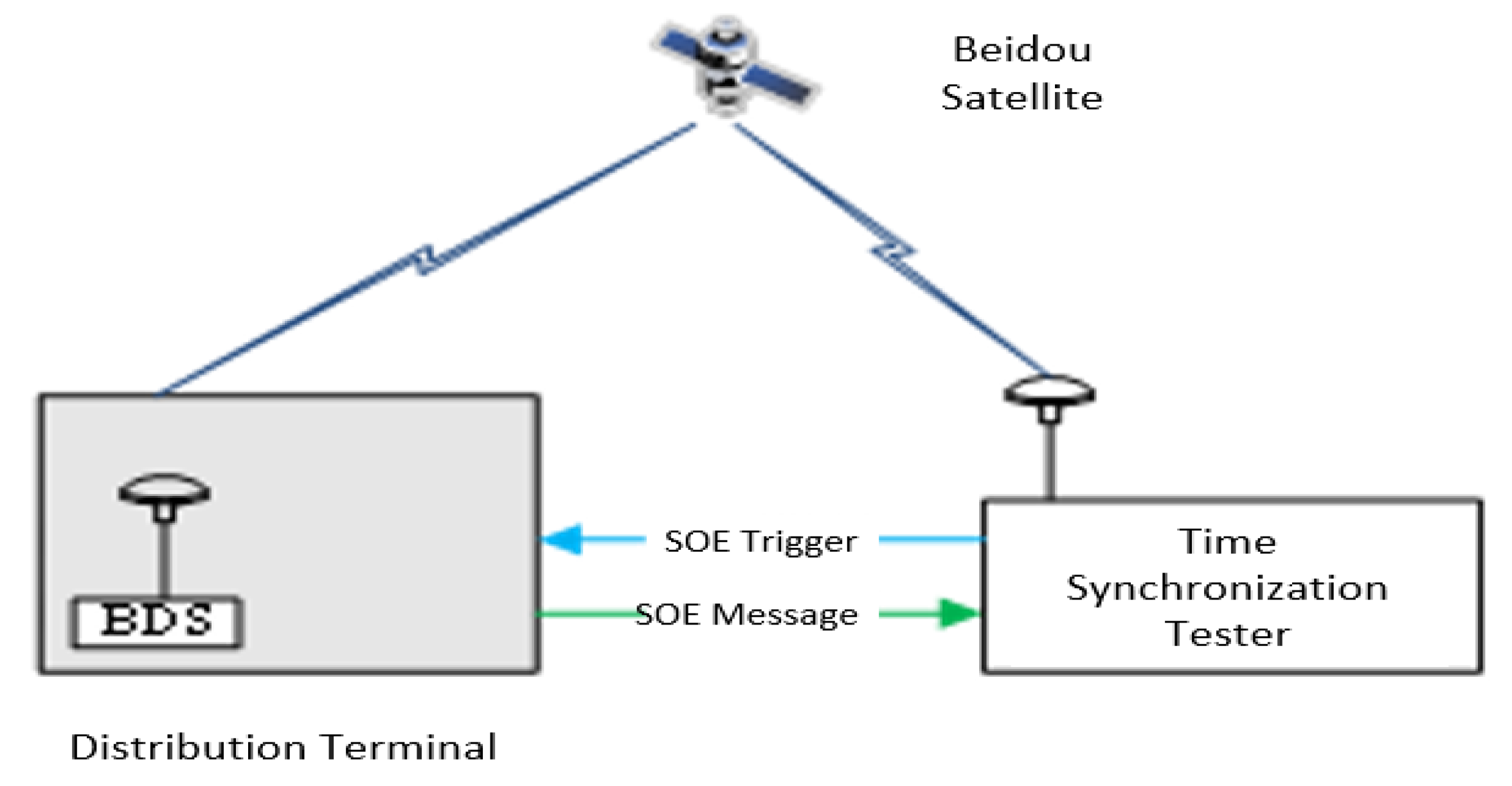
Test method
1.Distribution terminals A and B received BeiDou satellite signals and synchronized normally for 10 minutes;
2.Set the timed tripping moment for distribution terminal A and the timed closing moment for distribution terminal B via master station commands;
3.Tested the contact opening moment of circuit breaker A and the contact closing moment of circuit breaker B using a time synchronization tester;
4.Compared the time difference between the contact opening moment of circuit breaker A and the contact closing moment of circuit breaker B;
5.Repeat the test 10 times.
Experimental data
Table 7.
Accuracy test data for timed action of distribution terminals.
| NO. | The moment when Circuit Breaker A opens | Closing time of Circuit Breaker B | Time difference (ms) | Is the difference between the switch operation time and the model prediction time less than 0.1 milliseconds |
|---|---|---|---|---|
| 1 | 8:50:27.244 | 8:50:27.251 | 7 | Yes |
| 2 | 8:52:51.831 | 8:52:51.841 | 10 | Yes |
| 3 | 9:04:10.433 | 9:04:10.443 | 10 | Yes |
| 4 | 9:09:11.311 | 9:09:11.316 | 5 | Yes |
| 5 | 9:15:10.211 | 9:15:10.223 | 12 | Yes |
| 6 | 9:20:20.430 | 9:20:20.433 | 3 | Yes |
| 7 | 9:25:40.556 | 9:25:40.559 | 3 | Yes |
| 8 | 9:29:30.466 | 9:29:30.477 | 11 | Yes |
| 9 | 9:35:10.876 | 9:35:10.879 | 3 | Yes |
| 10 | 9:40:20.431 | 9:40:20.438 | 7 | Yes |
Experimental conclusions
This paper validates the Bo-BiLSTM-based synchronous load transfer control method for distribution networks through 10 repeated experiments. Experimental results demonstrate that switch operation times align with model predictions, with all trip and close operation timing deviations controlled within 2–12 ms—fully meeting the 20 ms engineering requirement. This effectively mitigates circulating current risks, proving the proposed control strategy’s effectiveness and reliability.
6. Conclusions
This study proposes a switch timing prediction and synchronous control method for distribution networks based on Bayesian optimization of bidirectional long short-term memory networks (Bo-BiLSTM). It effectively addresses the challenges of high dispersion in switch operation timing and low prediction accuracy under distributed power source integration. By constructing precise simulation models and feature databases, combined with Bayesian hyperparameter optimization, the method significantly enhances BiLSTM’s predictive performance and generalization capability under limited samples. Furthermore, the prediction results are applied to load transfer control. A dynamic delay control strategy is proposed and experimentally validated to maintain the switching time difference within 2–12 ms, fully meeting engineering safety requirements and achieving an effective closed-loop from prediction to control. This method provides a reliable fault response and rapid self-healing control solution for distribution networks with high distributed energy ratios, combining theoretical innovation with practical engineering value. Future research will focus on enhancing model generalization across diverse topologies while exploring multimodal data fusion and online learning mechanisms to further strengthen the system’s adaptability and control robustness in real-world complex environments.
Author Contributions
Conceptualization, H.Z. and C.L.; methodology, C.L.; validation, H.Z. C.L. and W.L.; formal analysis, X.S.; investigation, Y.G.; resources, Y.G.; data curation, C.L.; writing—original draft, W.L. and C.L.; writing—review and editing, X.S.; visualization, Y.G.; supervision, H.Z.; project administration, H.Z.; funding acquisition, H.Z. All authors have read and agreed to the published version of the manuscript.
Funding
This research was funded by the project of State Grid Sichuan Electric Power Company Limited,, grant number 52199723001R.
Data Availability Statement
Data are contained within the article.
Acknowledgments
We are grateful to the reviewers for their comprehensive review of this manuscript, as well as for their insightful comments and valuable suggestions that have significantly contributed to enhancing the quality of our work.
Conflicts of Interest
The authors declare no conflicts of interest.
References
- Liu, Y., Zhang, J., & Wang, L. (2021). Switching time prediction in distribution networks with distributed generation using deep learning. Electric Power Systems Research, 190, 106842.
- Zhao, H., Li, X., & Chen, Y. (2020). A BiLSTM-based method for fault diagnosis and switching time prediction in smart grids. IEEE Transactions on Smart Grid, 11(5), 4321–4330.
- Wang, P., Zang, J., & Yan, R. (2018). Long short-term memory for machine remaining life prediction. Journal of Manufacturing Systems, 48, 78–86.
- Gugulothu, N., Tv, V., & Malhotra, P. (2018). Predicting remaining useful life using time series embeddings based on recurrent neural networks. International Journal of Prognostics and Health Management, 9(1).
- Lu, Q., Polyzos, K. D., Li, B., & Wang, X. (2023). Surrogate modeling for Bayesian optimization beyond a single Gaussian process. IEEE Transactions on Pattern Analysis and Machine Intelligence, 45(3), 2891–2904.
- Burke, J., & King, S. (2021). Edge tracing using Gaussian process regression. IEEE Transactions on Image Processing, 31, 138–148.
- Ma, Y., He, Y., Wang, L., & Zhang, J. (2022). Probabilistic reconstruction for spatiotemporal sensor data integrated with Gaussian process regression. Probabilistic Engineering Mechanics, 69, 103264.
- Hodson, T. O. (2022). Root mean square error (RMSE) or mean absolute error (MAE): When to use them or not. Geoscientific Model Development Discussions, 2022, 1–10.
- Alturki, A. Y., Alhussainy, A. A., Alghamdi, M. S., & Alshammari, B. (2024). A novel point of common coupling direct power control method for grid integration of renewable energy sources. Energies, 17(20), 5111.
- Raj, R. D. A., & Bhattacharjee, S. (2020). Short-circuit fault analysis of three-phase grid integrated photovoltaic power system. In 2020 International Conference on Power Electronics & IoT Applications in Renewable Energy and its Control (PARC) (pp. 231–236).
- WenJie, J., ChulWoo, K., & Yoshinao, G. (2022). Data normalization and anomaly detection in a steel plate-girder bridge using LSTM. ASCE-ASME Journal of Risk and Uncertainty in Engineering Systems, Part A: Civil Engineering, 8(1).
- Ran, J., Cui, Y., et al. (2022). Improved runoff forecasting based on time-varying model averaging method and deep learning. PLOS ONE, 17(9), e0274004.
- Hochreiter, S., & Schmidhuber, J. (1997). Long short-term memory. Neural Computation, 9(8), 1735–1780.
- Babu, G. S., Zhao, P., & Li, X. L. (2016). Deep convolutional neural network based regression approach for estimation of remaining useful life. In International Conference on Database Systems for Advanced Applications (pp. 214–228).
- Guo, L., Xing, S. B., Li, N. P., & Wang, H. (2017). Deep convolution feature learning for health indicator construction of bearings. In Prognostics and System Health Management Conference (pp. 318–323).
- Zhang, J., Liu, Y., & Wang, L. (2022). A switching time prediction method for distribution networks based on Bayesian-optimized bidirectional LSTM. Electric Power Components and Systems, 50(3), 345–356.
Figure 1.
Distribution Network Simulation Model Diagram.
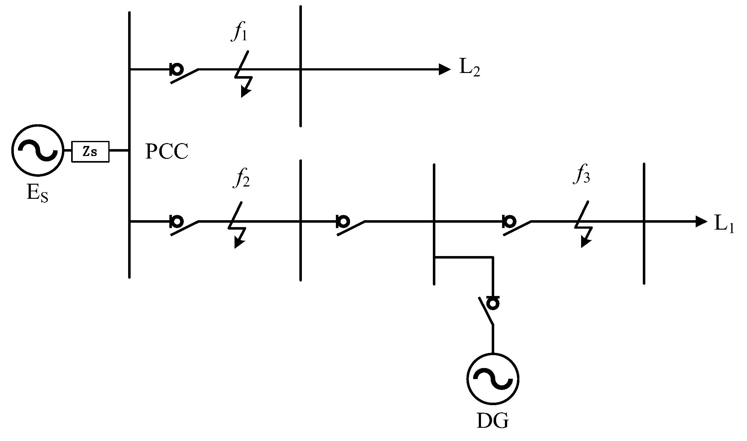
Figure 2.
BiLSTM Architecture Diagram.
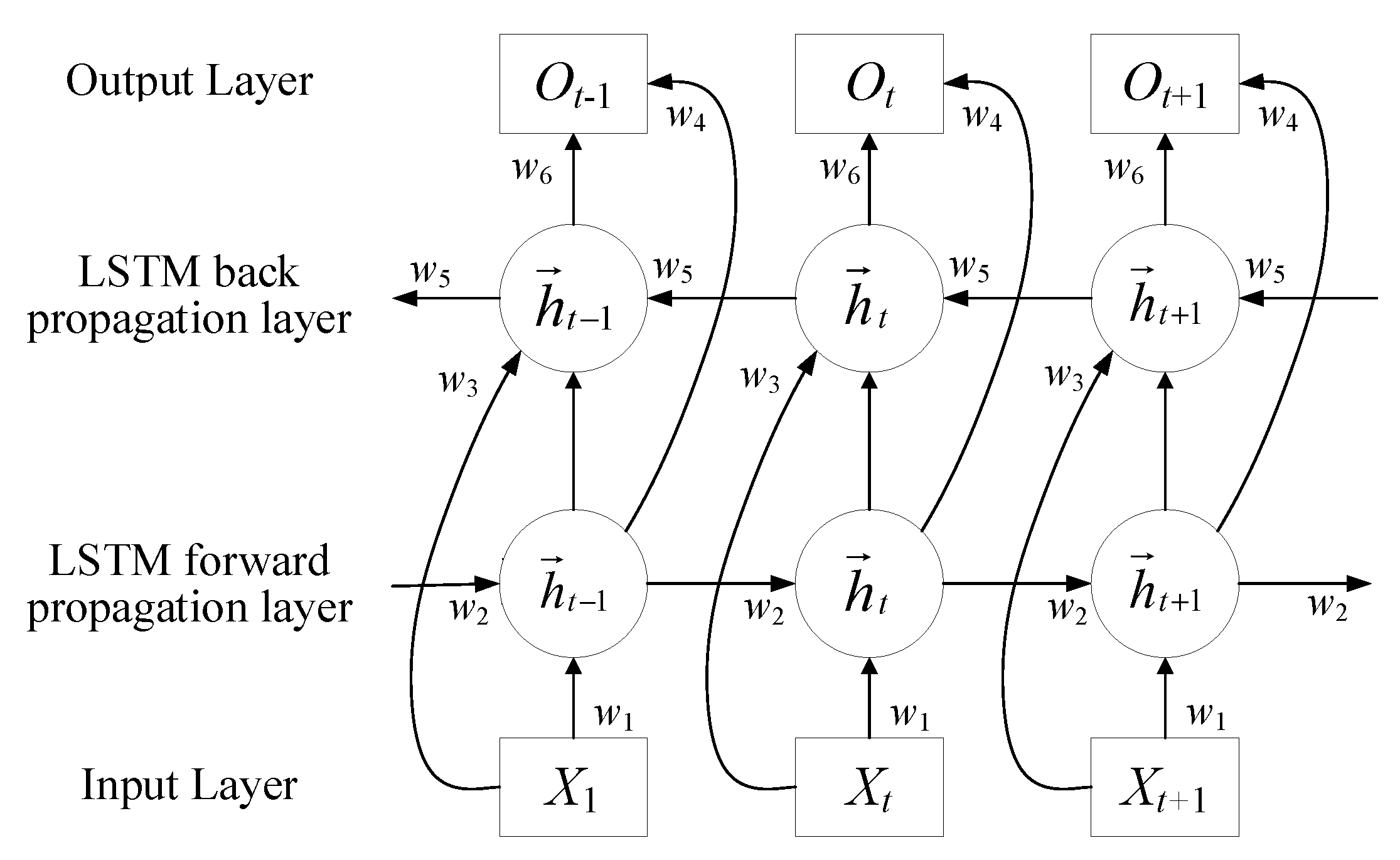
Figure 3.
Bo-BiLSTM Prediction Model Workflow.
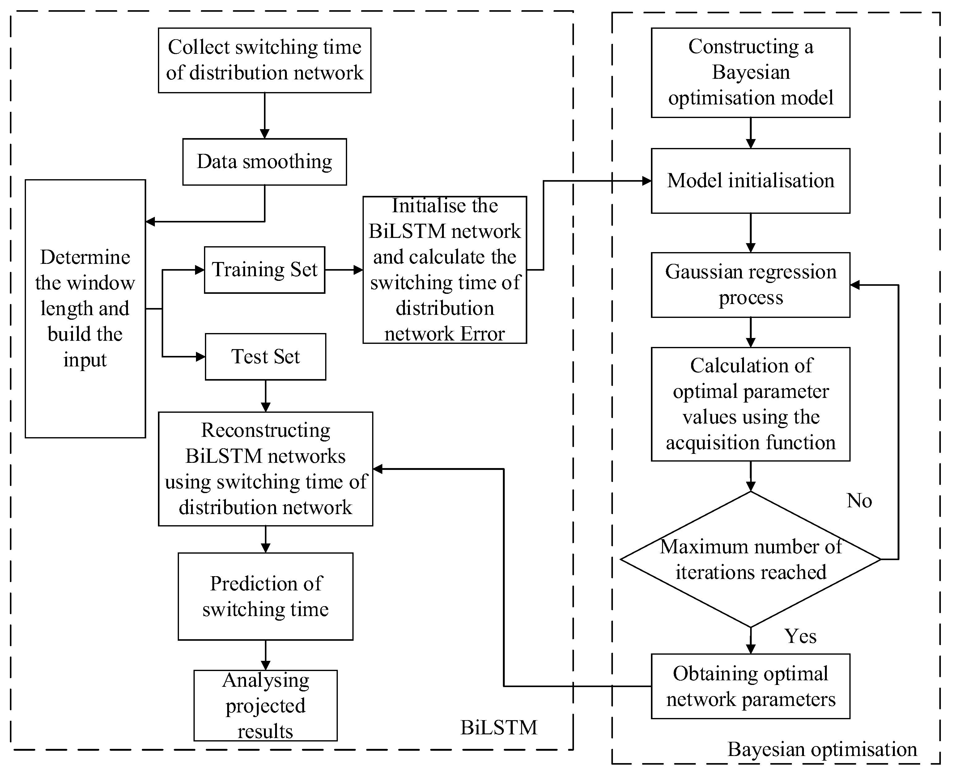
Figure 4.
Results of Bayesian optimization.
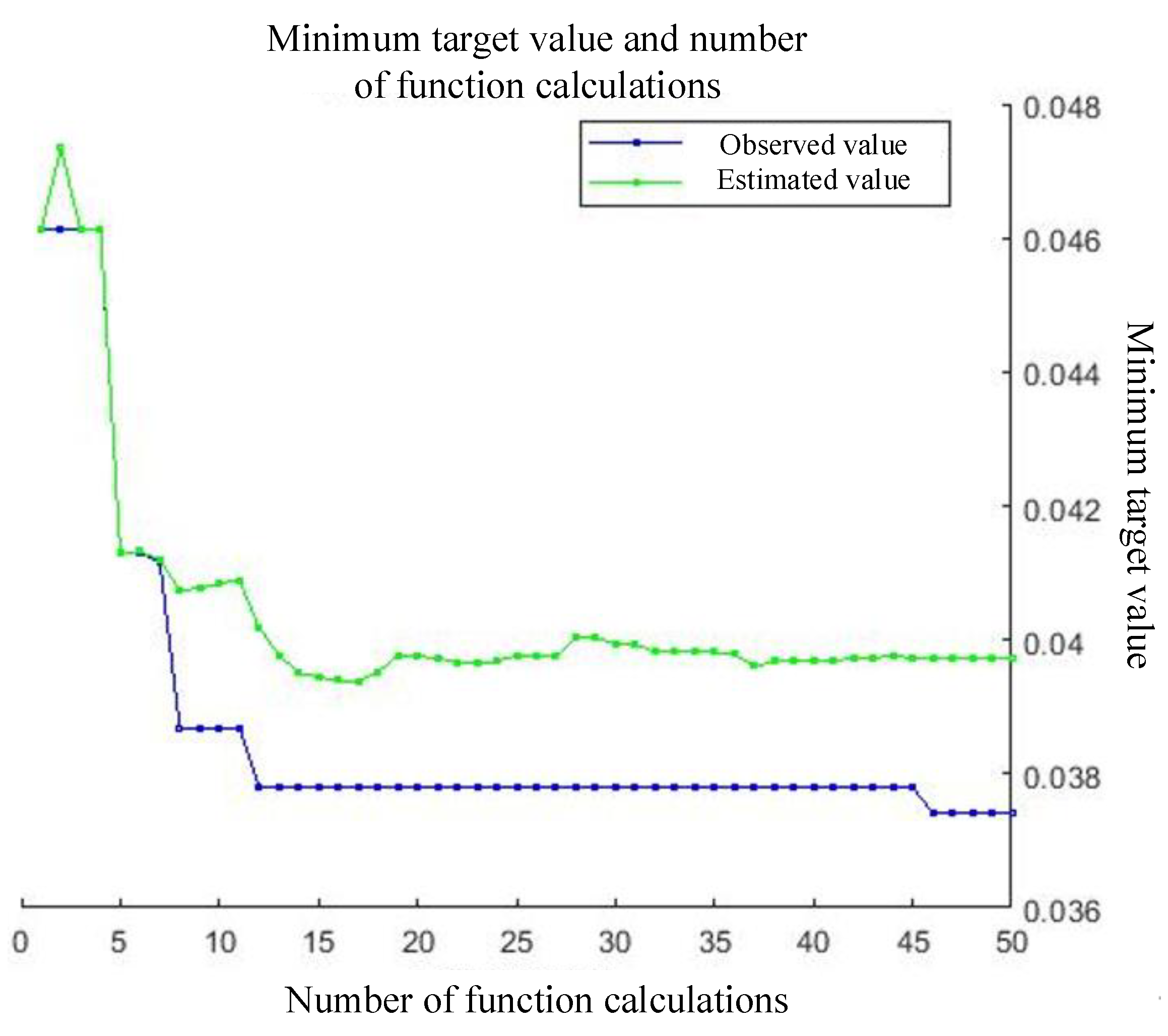
Figure 5.
Prediction Results of Switch Operation Times in Distribution Networks Using the Bo-BiLSTM Network Model.
Figure 5.
Prediction Results of Switch Operation Times in Distribution Networks Using the Bo-BiLSTM Network Model.
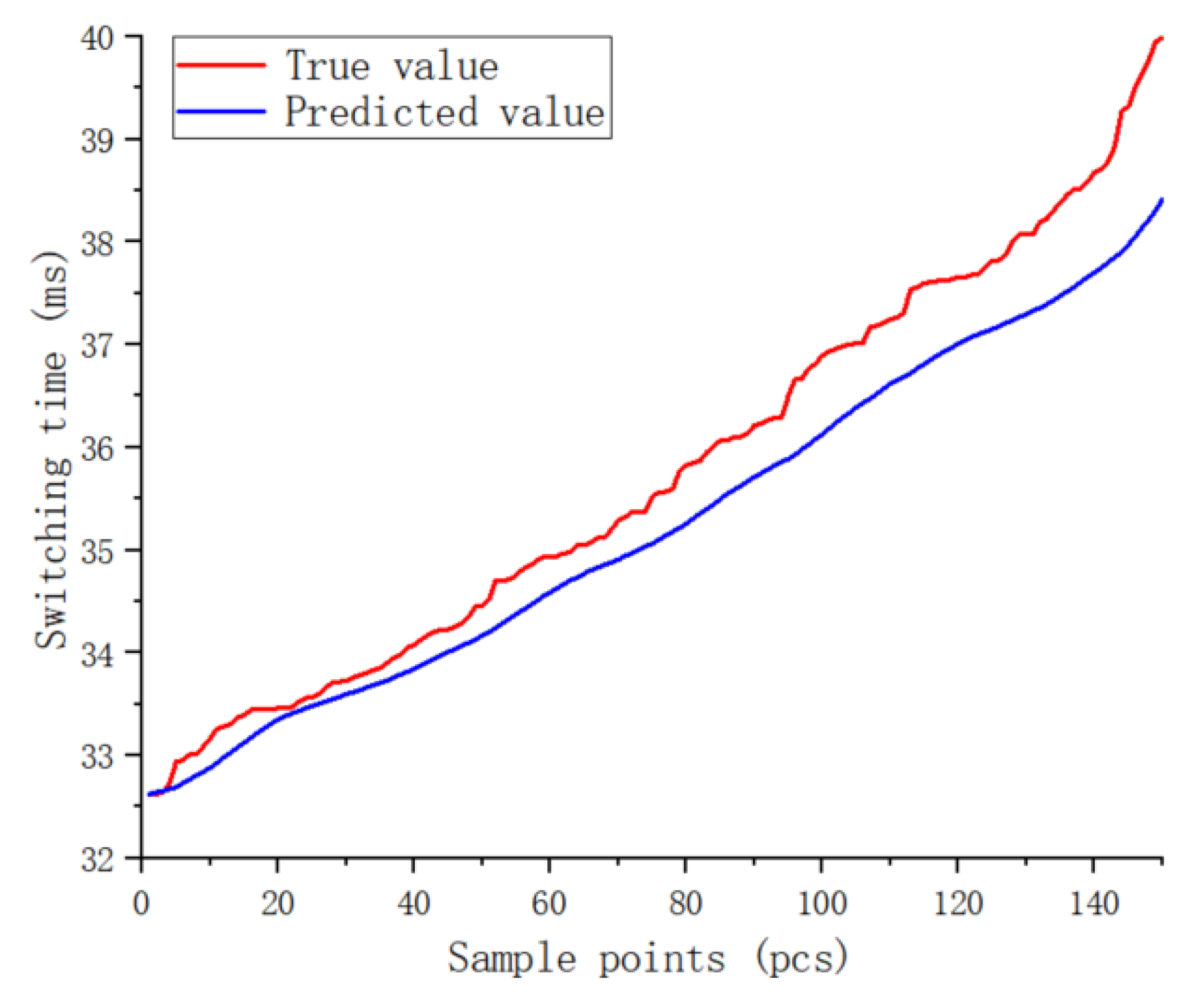
Figure 6.
Switching Time Prediction Results for Distribution Networks Using the BiLSTM Network Model.
Figure 6.
Switching Time Prediction Results for Distribution Networks Using the BiLSTM Network Model.
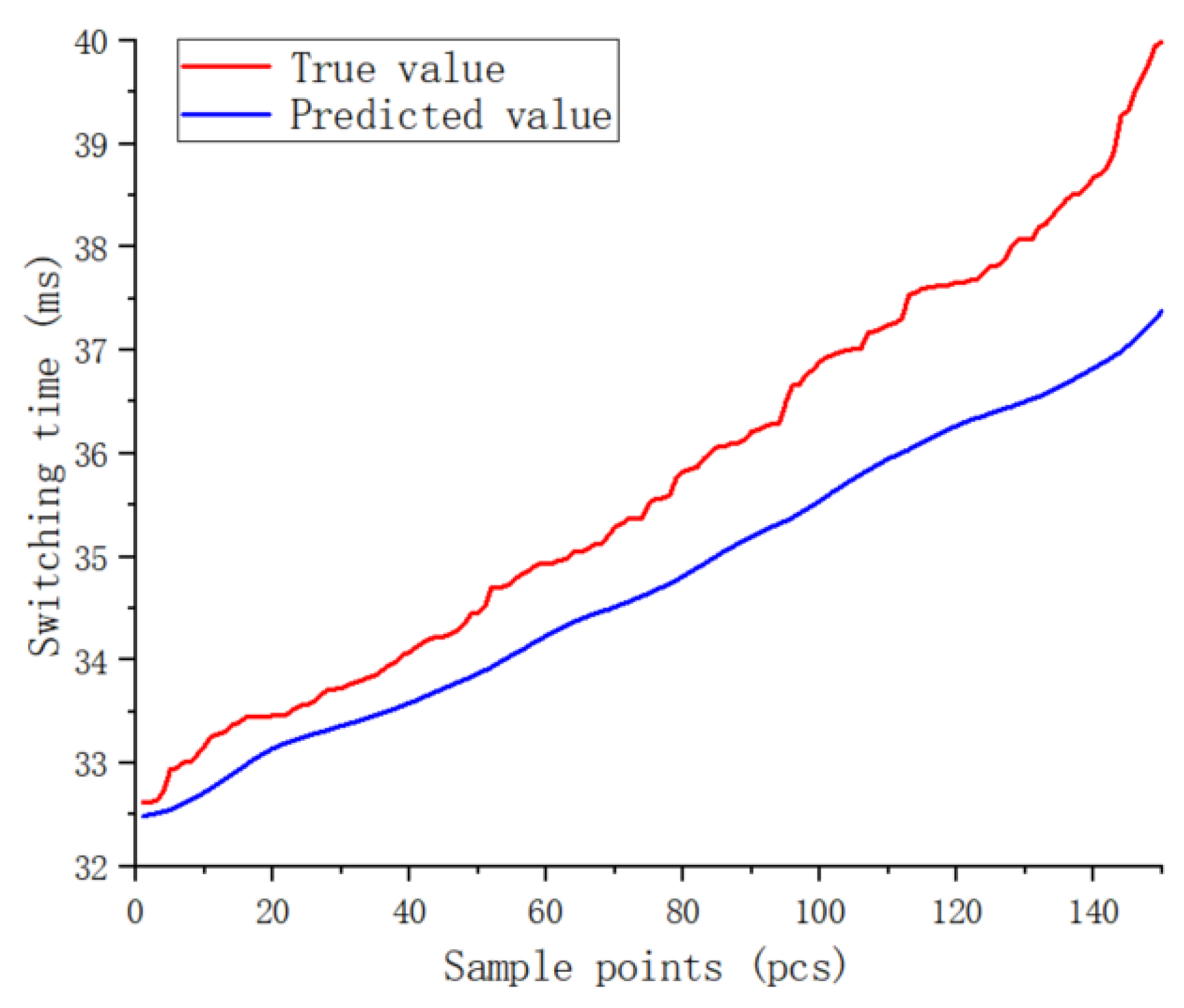
Figure 7.
Distribution Network Switching Time Prediction Results from the LSTM Network Model.
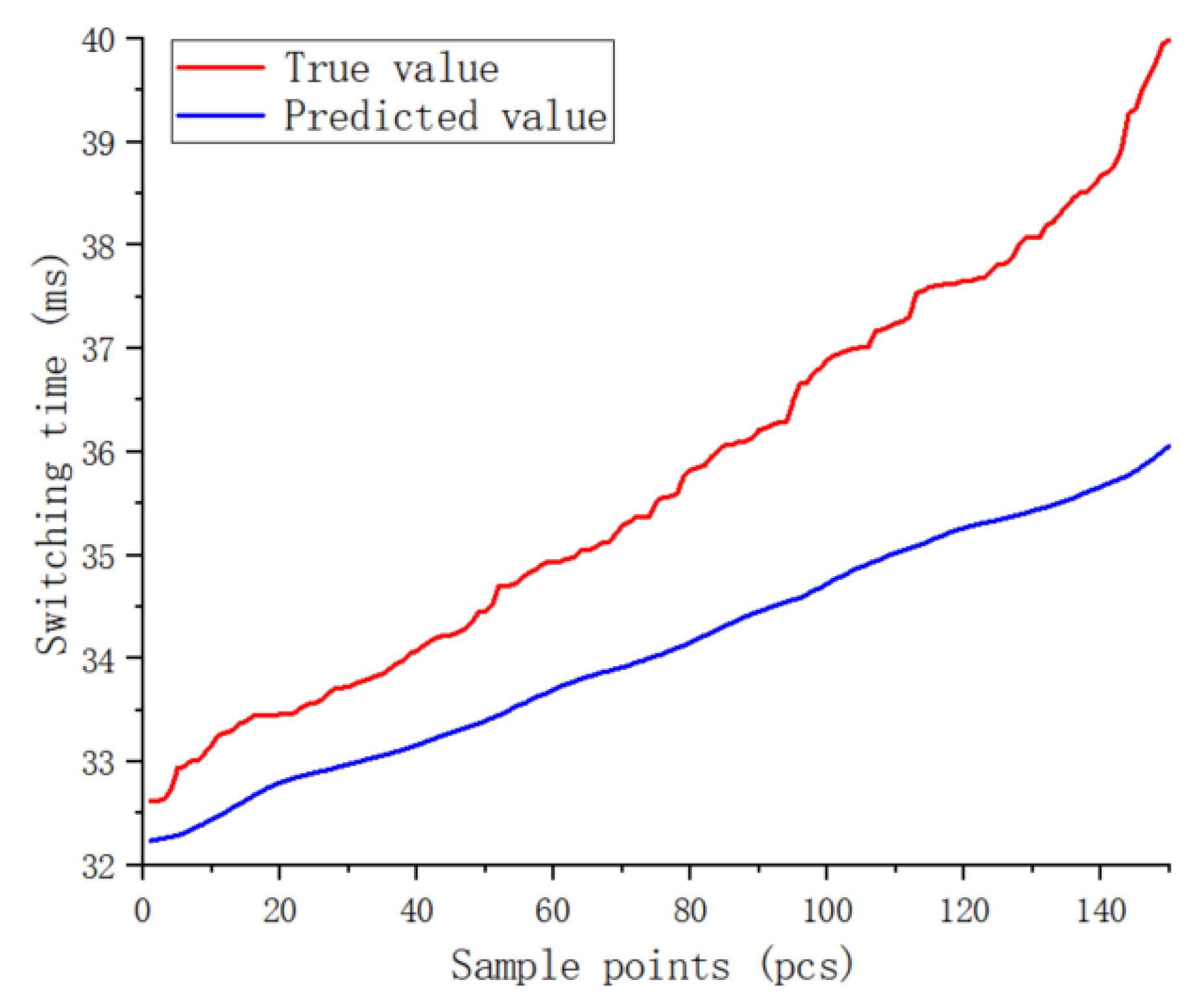
Table 1.
System Parameters Table.
| Parameter | value |
|---|---|
| Distributed power supply access location | Distribution network feeder non-terminal bus |
| Line positive sequence impedance/(Ω·km-1) | 0.27+j0.335 |
| Active power /kW | PL1=PL2=300 |
| Reactive power /kvar | QL1=QL2=130 |
| Fault type | Single-phase short circuit, two-phase short circuit, two-phase ground short circuit, three-phase short circuit and three-phase short circuit grounding |
| Fault location | f1、f2、f3 |
| Grounding transition resistance /Ω | 0.001、25、50、100 |
| Duration of the fault /s | 0.5 |
| Photovoltaic Capacity/kW | 213.15 |
| L1, L2 ,Length/km | 300、100 |
| Power Supply Rated Voltage/kV | 35 |
| Power Supply Rated Capacity/kVA | 630 |
| Zs/Ω | 0.8929+j5.209 |
Table 3.
Fault characteristic data under different operating conditions.
| Operating order number | VA /(V) | VB /(V) | VC /(V) | IA /(A) | IB /(A) | IC /(A) | T/(ms) |
|---|---|---|---|---|---|---|---|
| O1 | 28140 | 28760 | 28780 | 106.4 | 40.78 | 35.07 | 26.04 |
| O2 | 28750 | 27500 | 28790 | 33.38 | 276.7 | 42.67 | 37.60 |
| O3 | 28730 | 28740 | 28730 | 35.99 | 36.01 | 35.99 | 31.70 |
| O4 | 28730 | 28750 | 26540 | 36.92 | 36.35 | 388.9 | 16.85 |
| O5 | 28740 | 28790 | 27970 | 40.8 | 37.22 | 119.2 | 27.73 |
| ⁝ | ⁝ | ⁝ | ⁝ | ⁝ | ⁝ | ⁝ | |
| O310 | 28730 | 27250 | 25710 | 35.96 | 574.3 | 542.7 | 36.891 |
Table 4.
Normalized database of eigenmatrix.
| VA | VB | VC | IA | IB | IC | |
| O1 | 0.4144 | 0.9822 | 0.9911 | -0.8120 | -0.9799 | -0.9945 |
| O2 | 0.6390 | 0.4209 | 0.9956 | -0.9988 | -0.3763 | -0.9751 |
| O3 | 0.6317 | 0.9733 | 0.9689 | -0.9921 | -0.9921 | -0.9921 |
| O4 | 0.6317 | 0.9777 | -0.0044 | -0.9898 | -0.9912 | -0.0893 |
| O5 | 0.6354 | 0.9955 | 0.6311 | -0.9798 | -0.9890 | -0.7793 |
| ⁝ | ⁝ | ⁝ | ⁝ | ⁝ | ⁝ | ⁝ |
| O310 | 0.6317 | 0.3096 | -0.3733 | -0.9922 | 0.3850 | 0.3042 |
Table 5.
Comparison of Prediction Metrics for Distribution Network Switch Operation Time Prediction Models.
Table 5.
Comparison of Prediction Metrics for Distribution Network Switch Operation Time Prediction Models.
| Model | R2 | RMSE | MAE |
|---|---|---|---|
| Bo-BiLSTM | 0.90401 | 0.59982 | 0.49864 |
| BiLSTM | 0.61915 | 1.1948 | 1.035 |
| LSTM | 0.54711 | 1.3029 | 1.1145 |
Table 6.
Bo-BiLSTM Network Model Prediction Error Table.
| Model | True value | Predicted value | Absolute value error |
|---|---|---|---|
| Bo-BiLSTM | 36.88883 | 36.12697 | 0.76186 |
| BiLSTM | 36.88883 | 35.54005 | 1.34878 |
| LSTM | 36.88883 | 34.72493 | 2.1639 |
Disclaimer/Publisher’s Note: The statements, opinions and data contained in all publications are solely those of the individual author(s) and contributor(s) and not of MDPI and/or the editor(s). MDPI and/or the editor(s) disclaim responsibility for any injury to people or property resulting from any ideas, methods, instructions or products referred to in the content. |
© 2025 by the authors. Licensee MDPI, Basel, Switzerland. This article is an open access article distributed under the terms and conditions of the Creative Commons Attribution (CC BY) license (http://creativecommons.org/licenses/by/4.0/).
Copyright: This open access article is published under a Creative Commons CC BY 4.0 license, which permit the free download, distribution, and reuse, provided that the author and preprint are cited in any reuse.


