
Submitted:
14 January 2025
Posted:
14 January 2025
You are already at the latest version
Abstract
The findings of this study underscore the efficacy of integrating the time modelling capability of LSTM with the robustness of integrated methods to enhance the stability and operational reliability of the power grid. This study has contributed to the development of elastic DSE technology that can adapt to the complexity challenges of modern power grids.
Keywords:
Dynamic State Estimation
; Machine Learning
; Data Loss
; Power Systems
; Neural Networks
; Ensemble Methods
1. Introduction
Accurate dynamic state estimation (DSE) is essential for ensuring the stability and reliability of power systems. With the increasing complexity of modern microgrids, influenced by renewable energy sources and distributed generation, maintaining robust state estimation under real-world constraints such as data loss[1] has become a pressing challenge . Communication constraints [2], particularly in periods of congestion or instability, can lead to data dropouts, degrading the performance of conventional estimation methods and posing risks to power system operations .
Recent studies have explored methods to mitigate these issues, including the application of Markov models like the Gilbert-Elliott model to describe packet loss behavior[3]. Machine learning (ML) approaches, such as neural networks[4] and ensemble learning[5], have shown promise in enhancing the accuracy of state estimation despite data lose. However, the effectiveness of different ML models under such conditions is still a topic of ongoing research and debate.
This study aims to provide a comparative analysis of nine machine learning methods for DSE in data loss scenarios: random forest regression, AdaBoost regression, gradient boosting regression, ExtraTrees regression, CatBoost regression, K-nearest neighbor (KNN) regression, XGBoost regression, LightGBM regression, and linear regression (using gradient descent). In addition, we enhance the neural network architecture with residual connection and self-attention mechanism consisting of 3 LSTMs[6] and 3 FNNs to further improve the robustness of the estimation.
Our findings reveal the most effective algorithms for mitigating the impact of data loss on dynamic state estimation, offering insights into practical applications for power system stability. This work contributes to the ongoing effort to develop resilient estimation techniques that can adapt to the challenges of modern power grids.
2. Materials and Methods
2.1. System Model and Data Generation
The study uses the Kundur’s two-area, four-machine power system model to simulate dynamic states of a power system under varying operational conditions[7]. This system model is widely recognized for evaluating stability and dynamic response in power system research. The simulations were performed using standard power system simulation software to generate datasets that include the following generator states:Rotor Angle (δ);Rotor Speed (ω);Transient Voltage (E’).
The inputs include excitation voltage (Efd) and mechanical power (Pm). The corresponding measurements consist of active power (Pe), reactive power (Qe), terminal voltage (Vt), and terminal current (It).
2.2. Data Loss Simulation
To simulate real-world communication constraints, data dropouts were modeled using the Gilbert-Elliott model. This model represents the communication channel as a two-state Markov chain with: Good State (0): Successful data transmission.; Bad State (1): Data loss (packet loss).;The transition probabilities between states were predefined based on historical data. The state transition matrix is given by:
2.3. Machine Learning Methods
Nine machine learning algorithms were employed to estimate the dynamic states of the power system under data loss conditions. These methods are: Random Forest Regression (RF)[8,9];AdaBoost Regression; Gradient Boosting Regression (GBR); ExtraTrees Regression;CatBoost Regression; K-Nearest Neighbors (KNN) Regression; XGBoost Regression; LightGBM Regression; Linear Regression (Gradient Descent).
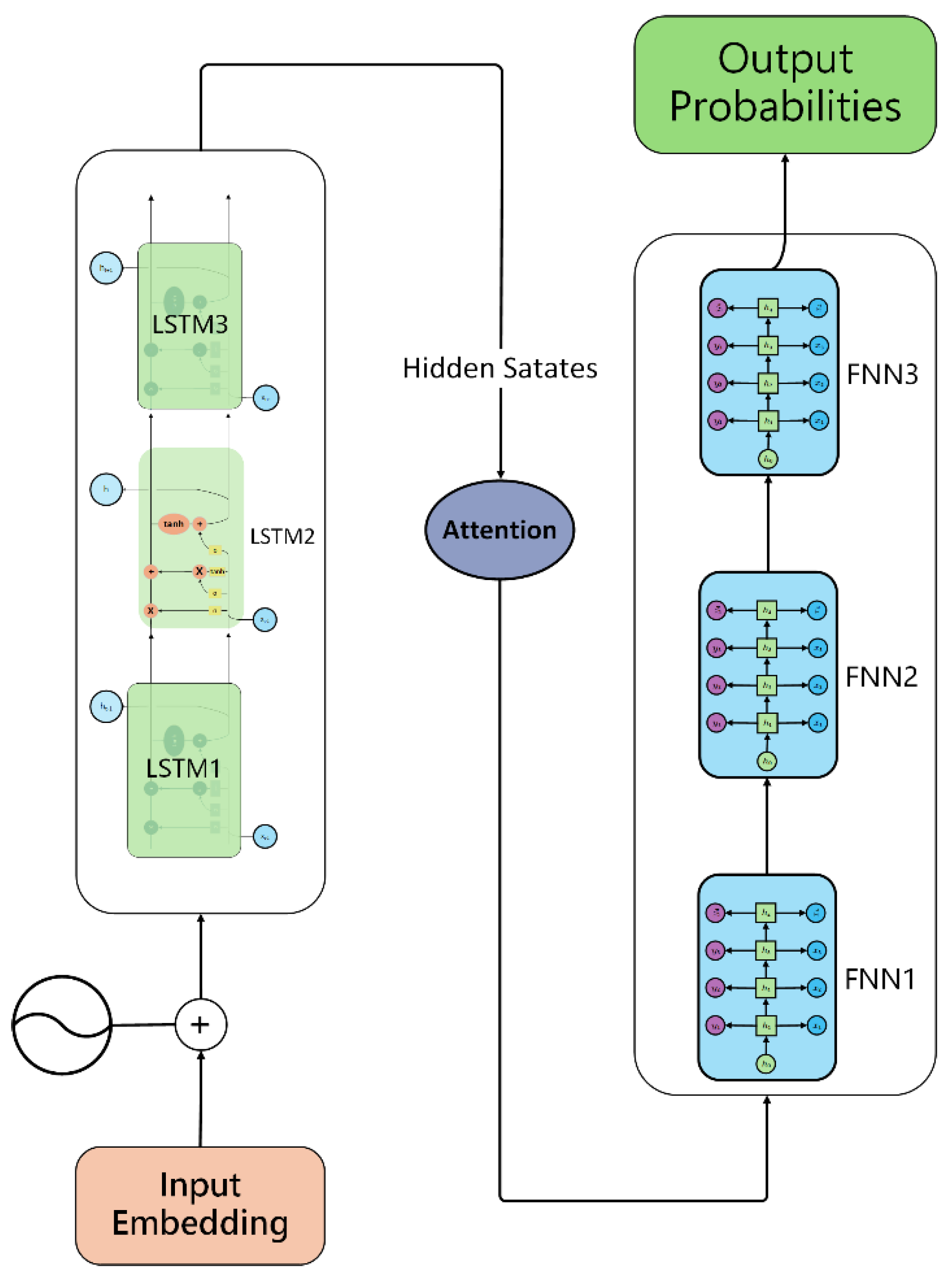
2.4. Neural Network Enhancements
For improved performance, the neural network architecture was enhanced with residual connections and a self-attention mechanism[10]. The architecture includes:
Two Long Short-Term Memory (LSTM) layers; Four Feedforward Neural Network (FNN)[11] layers; The neural network training process was divided into three stages:
First Stage: Train LSTM1, FNN1, and FNN2 without considering data loss.
Second Stage: Freeze the parameters of LSTM1, FNN1, and FNN2, then train LSTM2, FNN3, and FNN4 with the Gilbert-Elliott model integrated to simulate data loss.
Third Stage: Freeze all previous parameters and train a Random Forest Regressor on the final hidden states of FNN4.
Figure 1.
Improved neural network architecture.
3. Results
3.1. Comparative Analysis of Machine Learning Methods
The following machine learning models were tested for their ability to estimate the dynamic states of the system under data loss[12]: Random Forest Regression[8]; AdaBoost Regression[13]; Gradient Boosting Regression[14]; Extra Trees Regression[15]; CatBoost Regression[16]; K-Nearest Neighbors (KNN) Regression[17]; XGBoost Regression[18]; LightGBM Regression[19]; Linear Regression (Gradient Descent)[20].The performance metrics used for comparison were: Mean Relative Error (MRE)[21];Variance of the error distribution[22]. The results of the comparative analysis are summarized in Table 1.Performance of Machine Learning Models for Dynamic State Estimation under Data Loss
3.2. Figures, Tables and Schemes
The Table 1 lists three different machine learning models along with their parameters and corresponding values. Here's an analysis of each model and its parameters:
The input layer size is set to 1, indicating that only one feature is input at each time step. The hidden layer size is 512, meaning that each hidden layer contains 512 neurons. The number of layers is 4, suggesting that the LSTM network consists of 4 hidden layers. The sequence length is 50, which typically refers to the number of time steps in the input sequence. The learning rate, which is set to 2e-5, is utilised to regulate the rate at which the model updates its weights during the training process.
The output layer is characterised by a size of 1, signifying that the network produces a solitary output value. The network comprises a total of three layers, encompassing the input layer, a hidden layer, and the output layer. The learning rate is configured to 2e-5, aligning with the LSTM model, and it governs the rate at which weights are updated during the training process.
N_estimator: The number of estimators is 100, referring to the number of weak learners used in the AdaBoost algorithm. Learning rate: The value of the learning rate is 0.1, the function of which is to regulate the contribution of each weak learner. Random state: The random state is 42, which is employed to ensure the reproducibility of results, especially in the process of data splitting and model training.
These parameters are of pivotal significance for the performance and training process of the models. For instance, the size and number of hidden layers affect the complexity and learning capacity of the model, while the learning rate influences the stability and convergence speed during training. The parameters for the AdaBoost Regressor are outlined in Table 1.
The Table 2 illustrates three network models, accompanied by their associated parameters and corresponding values. The LSTM model is characterized by the following parameters: The input layer is sized 1, indicating that the dimension or the number of features of the input data is 1.The size of the hidden layers is 512, implying that each hidden layer contains 512 neurons. A larger hidden layer size may enable the model to learn more complex patterns, but it may also increase the computational cost and the risk of overfitting. The number of layers is 4. More layers allow the model to perform more in-depth feature extraction and learning, but it may also bring about problems such as overfitting, which requires appropriate regularization and other means to control. The length of the sequence is 50, which may be related to the sequential nature of the input data. In the context of time series data, for instance, 50 may denote the sequence length of 50 time steps input to the model on each occasion. The learning rate is set to 2e-5, a value which, while typically ensuring stability during training, can result in a reduced convergence speed. With regard to the FNN model:
The size of the hidden layer is 512, which has a similar impact on the model's learning ability as the hidden layer size of the LSTM. The output layer is 1, indicating that the output of this model is a single value, which may be suitable for regression and other tasks. The number of layers is 3, a relatively shallow network structure, which may have different trade-offs in learning ability and computational complexity.
The learning rate is set to 2e-5, and it is anticipated that this will have a comparable effect on the characteristics of the training process to that observed in the LSTM model. The N_estimator is set to 100, which may be indicative of the number of estimators in the model. For instance, in the context of ensemble learning, 100 base learners may be employed.
In the context of the Gradient Boosting Regressor model, the learning rate is set at 0.1, which is notably higher than the rates employed in LSTM and FNN models. This may result in more rapid weight updates during the training phase.
The Table 3 shows that the Input Layer Size is defined as follows: The input layer size is set to 1, indicating that the network processes a single feature at each time step, a common configuration for univariate time series data.
Hidden Layer Size: The hidden layer size is set to 512, suggesting a substantial capacity for the network to capture complex patterns within the data through a significant number of neurons. Number of Layers: With four layers specified, the LSTM network is configured to have multiple hidden layers, which can enhance its ability to learn and represent temporal dependencies in the data. Learning Rate: The learning rate is set to 2e-5, a conservative value that ensures the model's weights are updated gradually during training, potentially leading to more stable convergence and preventing overshooting. Finally, the sequence length is set to 50, which is a standard value that allows the network to effectively utilise a moderate range of past data points when making predictions. The sequence length is set to 50, which defines the number of time steps that the LSTM considers when making predictions, allowing it to leverage information from a moderate window of past data points.
This format provides a clear and concise description of each hyperparameter, explaining its role and the implications of its value in the context of the LSTM network's performance.
The Table 4 presents three network models (LSTM, FNN, KNN) along with their relevant parameters and corresponding values.
The table summarizes key hyperparameters for LSTM, FNN, and KNN models, highlighting LSTM's deep architecture with 4 layers and a hidden size of 512 for complex temporal data processing, FNN's single output for regression tasks with a similar hidden size, and KNN's flexible boosting stages and learning rates suited for diverse regression challenges, with a focus on balancing model complexity and performance.
The Table 5 details the configurations of three machine learning models. The LSTM, designed for temporal data, has an input layer for a single feature, 512-neuron hidden layers across 4 layers, and a sequence length of 50, with a 2e-5 learning rate for stable training. The FNN, with a comparable 512-neuron hidden layer, features a [4,4,3] layered structure for complex data representation and shares the LSTM's learning rate. The K-Neighbors Regressor is configured with 5 neighbors to balance local data consideration with generalization. These settings are tailored for optimal learning and prediction accuracy across the models.
As illustrated in Table 6, three network models (LSTM, FNN, Cat Boost Regressor) are presented, accompanied by their respective parameters and values.
For the LSTM model, the input layer size is set to 1, denoting the dimension or feature count of the input data.The size of the hidden layer is 512, which, although larger sizes may facilitate the learning of complex patterns, can increase costs and the risk of overfitting.The layers are as follows: 4, for in-depth feature extraction and learning, may cause overfitting.he sequence length of 50 is related to the input data's sequential nature.The learning rate of 2e-5 is a crucial parameter, as it ensures stability during training while moderating convergence.
For the Feedforward Neural Network (FNN):Hidden layer size: 512, similar impact on learning ability.The output layer: 1, which is suitable for regression.The layers are as follows: [3, 3, 4], with trade-offs in learning and complexity.The learning rate of 2e-5 has a discernible impact on the training process.The iterations are as follows: 1000, with the possibility of overfitting or prolonged training with higher values.
For the Cat Boost Regressor:Learning rate: 0.1, a larger value may facilitate more rapid weight updates but can also result in oscillations.The depth parameter, set at 6, has been observed to facilitate the learning of complex relationships; however, it has also been noted to increase the risk of overfitting.Finally, the verbosity parameter, set at 100, is related to the degree of information provided by the model.
It is imperative to note that these settings have a profound impact on the performance of the model, its operational speed, and its capacity for generalisation. It is recommended that these settings be adjusted and optimized based on the specific characteristics of the data and the intended tasks, with the objective of achieving the best possible outcome. In this regard, it is essential to take into account factors such as the complexity of the data, the available computing resources, and the associated time costs.
The Table 7 provides a concise overview of the hyperparameter settings for three machine learning models: LSTM, FNN, and Gradient Boosting Decision Tree. The LSTM model is configured with an input layer size of 1, 512 neurons in the hidden layers, 4 layers deep, a sequence length of 50, and a learning rate of 2e-5, making it suitable for capturing temporal dependencies in data. The FNN, with a single output and 512 neurons in its hidden layer, is set with 3 layers and the same learning rate of 2e-5 as the LSTM, indicating a design for complex pattern recognition with a focus on regression tasks. The Gradient Boosting Decision Tree is parameterized with 100 estimators, a learning rate of 0.1, a maximum depth of 3, and a random state of 42, which suggests a robust setup for handling various types of data and avoiding overfitting through controlled randomness. These configurations highlight a balance between model complexity and generalization capabilities.
The provided Table 8 outlines the optimized hyperparameters for three machine learning models: LSTM, FNN, and Optimal Random Forest Regressor. The LSTM configuration is designed to handle time-series data effectively, with an input layer dimension of 2, a substantial hidden layer size of 256, a model depth of 4 layers, a sequence length of 5, and an aggressive learning rate of 1e-4 to facilitate faster convergence. The FNN, with its 256-neuron hidden layer, single output neuron, and a total of 3 layers, is configured with a conservative learning rate of 2e-5, likely to ensure stable learning for its regression tasks. The Optimal Random Forest Regressor stands out with a high number of 1316 estimators, a considerable depth of 312, and specific criteria for minimum leaf size (5) and minimum split (2), suggesting a model that has been meticulously tuned for accuracy and generalization. This ensemble model's parameters indicate a preference for a complex model structure to capture intricate data relationships.
The Table 9 presents three network models (LSTM, FNN, XG-Boost Regressor) along with their relevant parameters and corresponding values.
For the LSTM model: The size of the input layer is 1, indicating that the dimension or the number of features of the input data is 1.The size of the hidden layers is 512, meaning each hidden layer has 512 neurons. A larger hidden layer size may enable the model to learn more complex patterns, but it may also increase the computational cost and the risk of overfitting. The number of layers is 4. More layers allow the model to perform more in-depth feature extraction and learning, but it may also bring about issues such as overfitting, which requires appropriate regularization and other means to control. The length of the sequence is 49, which may be related to the sequential nature of the input data. For example, when dealing with time series data, 49 may represent the sequence length of 49 time steps input to the model each time. The learning rate is 2e-5. A smaller learning rate usually makes the training process more stable, but it may lead to a slower convergence speed.
For the FNN model: The size of the hidden layer is 512, which has a similar impact on the model's learning ability as the hidden layer size of the LSTM. The output layer is 1, indicating that the output of this model is a single value, which may be suitable for regression and other tasks. The number of layers is 5, a relatively deeper network structure, which has different trade-offs in learning ability and computational complexity. The learning rate is 2e-5, and the characteristics of the training process will be similarly affected N estimators is [100, 200], which may be related to the range of the number of estimators in the model.
3.2. Comparison of the effectiveness of different machine learning algorithms
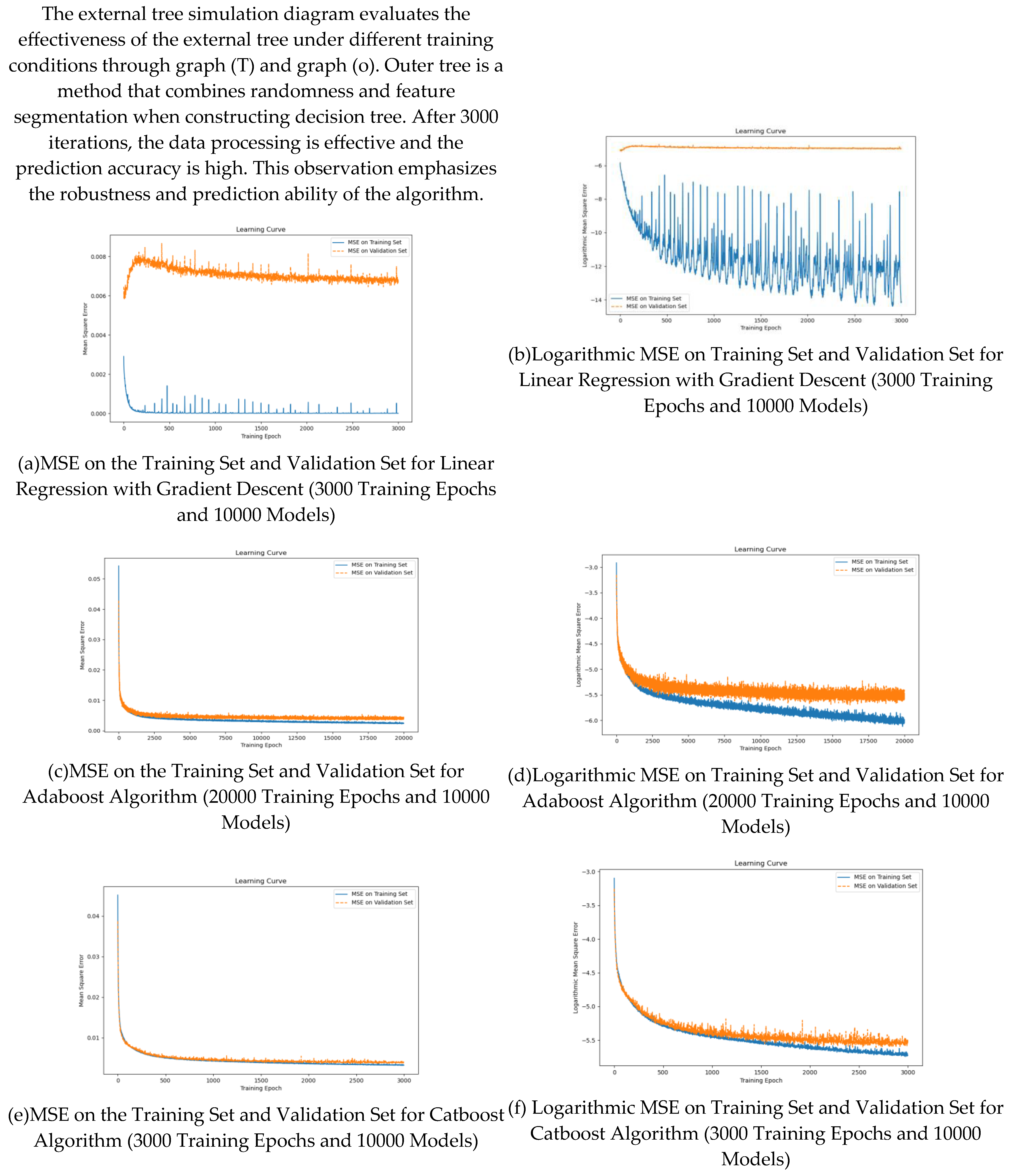
The Figures (a) and (b) illustrate the training process of linear regression model using gradient descent. As the number of iterations increases, the loss function decreases significantly, indicating that the model gradually learns and adapts to the data set. When the number of iterations reaches 3000, the model converges to the minimum loss value, which indicates that it successfully captures the linear relationship in the data and is ready for the accurate prediction task.
The performance trajectory of AdaBoost algorithm is shown in figures (c) and (d). The ensemble method aggregates weak learners into robust classifiers. With the increase of the number of weak learners, the classification accuracy is significantly improved. At 3000 iterations, the accuracy of the model is stable at a significant high level, which emphasizes the effectiveness of AdaBoost in enhancing the collective prediction ability of multiple weak classifiers to improve the overall performance.
Figures (E) and (f) show the performance of catboost in different training operations. The model can deal with classification features well, and the prediction error decreases with the increase of iteration times. After 3000 iterations, the model achieved satisfactory results, effectively managed the classification input, and provided accurate prediction.
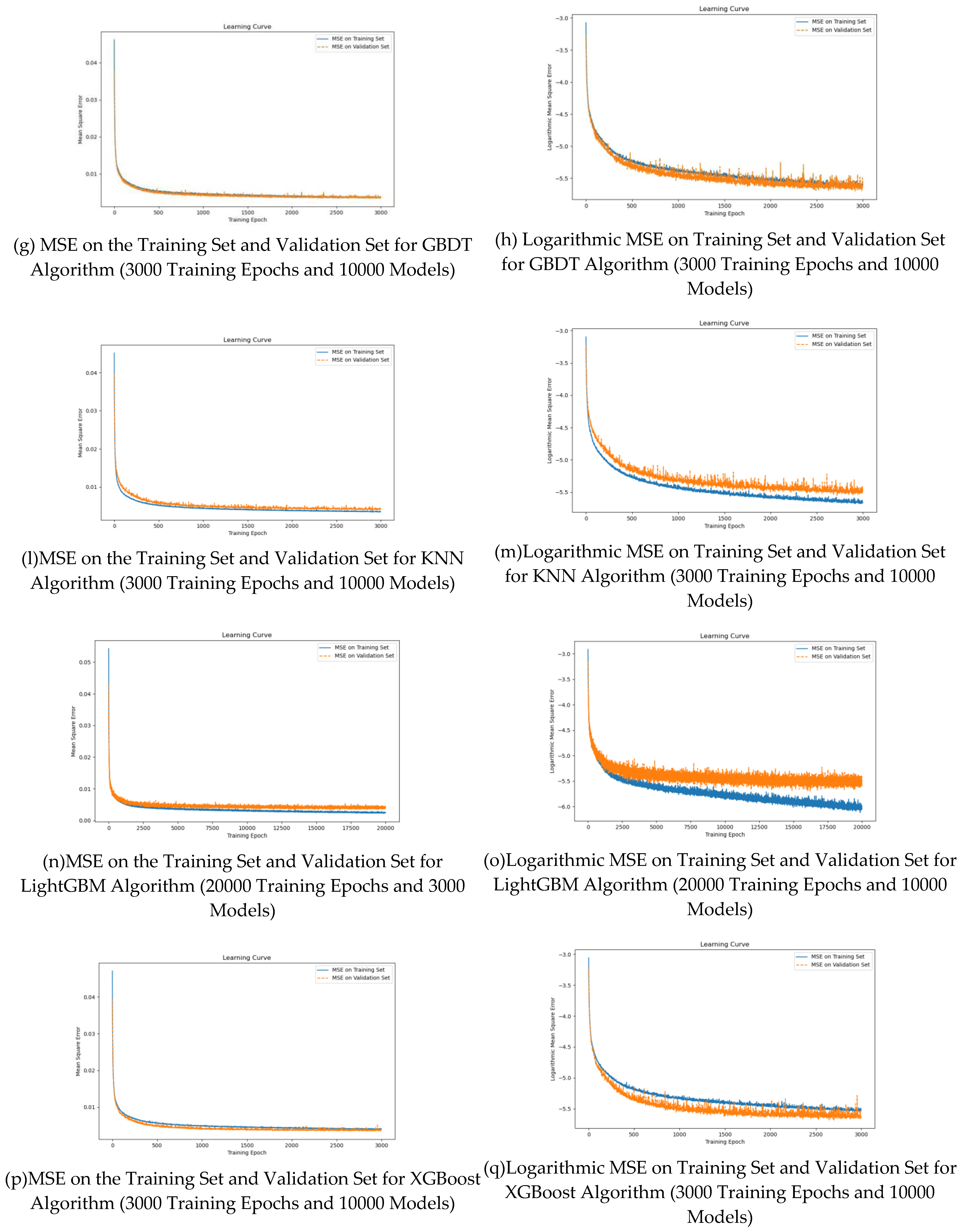
Gbdt simulation diagrams (g) and (H) illustrate the training dynamics of the gradient lifting decision tree algorithm. Gbdt is an integrated technology that gradually establishes a decision tree to improve prediction. The results show that the consistency of prediction error decreases with the increase of the tree. After 3000 experiments, gbdt successfully identifies the complex patterns in the data, which provides a solid foundation for reliable prediction results.
Figures (L) and (m) test the performance of KNN algorithm under different parameter configurations. KNN algorithm depends on the closeness between samples for classification or regression, and shows different prediction accuracy under different K values. Through 3000 iterations, the model can select the best K value according to the data distribution, so as to optimize the prediction performance.
Figures (n) and (o) show the effectiveness of lightgbm in different training iterations. A notable feature of lightgbm is its speed and memory efficiency. As the number of iterations increases to 20000, the prediction error of lightgbm decreases significantly, and the accuracy and stability of the model are improved.
The prediction performance of xgboost regression model in different training stages is described in detail with (P) and (q) labeled graphs. Xgboost is a machine learning algorithm known for its effectiveness in processing large-scale data. After 3000 iterations, the prediction error is significantly reduced. This decline means the effective fitting of data, and emphasizes the robust prediction ability of the algorithm.
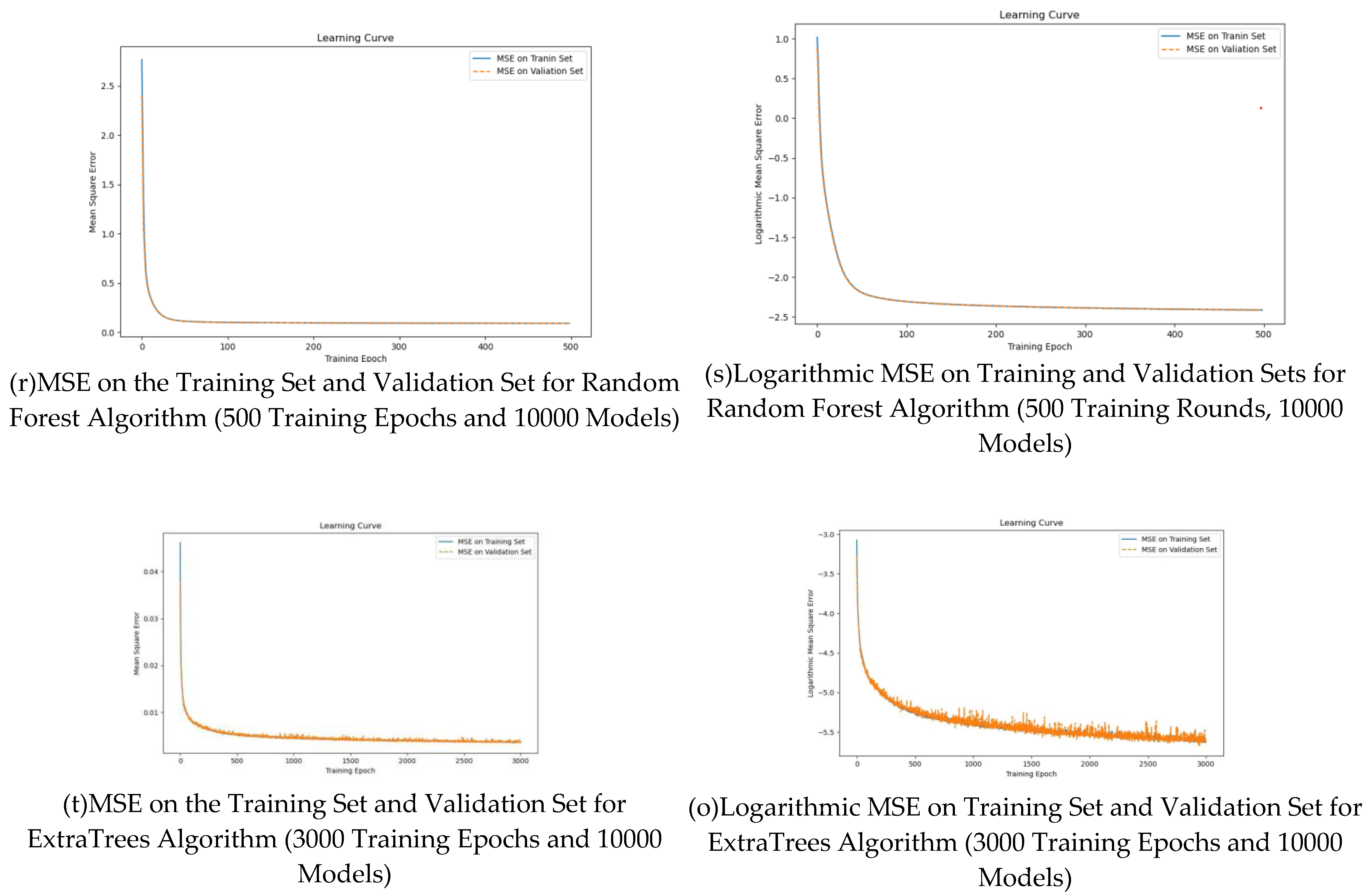
Stochastic Forest simulation is to train stochastic EST algorithm on a large number of data sets. The training results are shown in figures (R) and (s). Random forest algorithm is a comprehensive method that uses multiple decision trees to aggregate their predictions by voting or averaging. Experiments show that the algorithm achieves high prediction accuracy through 20000 data sets and 50000 iterations. The results show that the model can make full use of data information, reduce the over fitting ability, and produce reliable prediction results.
4. Discussion
Previous studies have primarily relied on traditional estimation techniques such as the Extended Kalman Filter (EKF) for DSE[23,24]. While EKF-based methods perform well under ideal communication conditions, they often fail to maintain accuracy during significant data loss [25]. For example, Zhao et al[23]. highlighted the limitations of EKF in scenarios with incomplete measurements and high communication latency. In this study, the ML-based approach incorporating the Gilbert-Elliott model for data loss simulation demonstrated greater robustness, offering a viable alternative to EKF-based methods.
The use of residual connections and self-attention mechanisms in the neural network architecture further enhanced the model's accuracy. These mechanisms, which have been successfully applied in other domains such as natural language processing and computer vision [26], improved the network’s ability to maintain stable learning and handle long-range dependencies in the data.
5. Conclusions
This article draws parallels between the performance of nine integrated machine learning methods for dynamic state estimation in power systems under data loss conditions. The methods under scrutiny include Random Forest Regression, AdaBoost Regression, Gradient Boosting Regression, Extra Trees Regression, CatBoost Regression, K-Nearest Neighbors Regression, XGBoost Regression, LightGBM Regression, and Linear Regression (using gradient descent). The study's background is rooted in the understanding that contemporary power grids have become intricate, particularly with the integration of renewable energy sources and distributed generation. This complexity renders accurate state estimation challenging in scenarios where communication constraints and data loss occur.The study utilised Kundur's two zone four machine power system model to simulate the dynamic state of power systems under diverse operating conditions, thereby generating pertinent datasets.The data loss simulation was executed using the Gilbert Elliott model, and the efficacy of the algorithms in mitigating the repercussions of data loss was assessed. Additionally, the study enhances the robustness of neural network architecture by incorporating residual connections and self-attention mechanisms.The simulation results demonstrate that the LSTM+FNN+RF method exhibits optimal performance, with an average relative error of 0.0854 and a variance of 0.6306. This outcome indicates that integrating the time modelling capability of LSTM with the robustness of integrated methods can enhance the stability and operational reliability of the power grid, providing solutions to the increasingly complex challenges in modern power systems.
6. Patents
We haven't started accepting it yet.
Author Contributions
Conceptualization, Yuefan Wang and Zhiyuan Luo; Methodology, Yuefan Wang; Software, Ruikai Feng; Verification, Yuefan Wang, Zhiyuan Luo, and Ruikai Feng; Formal analysis, Yuefan Wang; Investigation, Zhiyuan Luo; resources, Ruikai Feng; Data organization, Yuefan Wang; Writing - initial draft writing, Yuefan Wang; Writing - Review and Editing, Qi Zeng; Visualization, Yuefan Wang; Supervision, Qi Zeng; Project management, Qi Zeng; Obtaining funds, Qi Zeng. All authors have read and agreed to publish the manuscript version.
Funding
This research received no external funding.
Data Availability Statement
The generation of new data was not a feature of the process.
Conflicts of Interest
The authors declare no conflicts of interest.
References
- Yuchen Z, Yan X, Rui Z, Zhao Y D, et al. A Missing-Data Tolerant Method for Data-Driven Short-Term Voltage Stability Assessment of Power Systems[J]. IEEE Transactions on Smart Grid, 2018, 10, 5663–5674.
- Larissa S M Sugai. Pandemics and the Need for Automated Systems for Biodiversity Monitoring[J]. Journal of Wildlife Management, 2020, 84, 1424–1426.
- Yuxuan S, Zidong W, Bo S, Fuad E A, et al. Nonfragile H∞ Filtering for Discrete Multirate Time-delayed Systems over Sensor Networks Characterized by Gilbert-Elliott Models[J]. International Journal of Robust and Nonlinear Control, 2020, 30, 3194–3214. [CrossRef]
- Reihane R, Zhiwei G, Aihua Z, Richard B, et al. Robust Neural Network Fault Estimation Approach for Nonlinear Dynamic Systems with Applications to Wind Turbine Systems[J]. IEEE Transactions on Industrial Informatics, 2019, 15, 6302–6312. [CrossRef]
- Xianping Zhong, Heng Ban. Crack Fault Diagnosis of Rotating Machine in Nuclear Power Plant Based on Ensemble Learning[J]. Annals of nuclear energy, 2021, 168, 108909–108909.
- Wei F, Jinguang J, Shuangqiu L, Yilin G, Yifeng T, Yanan T, Peihui Y, Haiyong L, Jingnan L, et al. A LSTM Algorithm Estimating Pseudo Measurements for Aiding INS During GNSS Signal Outages[J]. Remote sensing, 2020, 12, 256–256. [CrossRef]
- Joakim B, Danilo O, Lennart H, Karl H J, et al. Influence of Sensor Feedback Limitations on Power Oscillation Damping and Transient Stability[J]. IEEE Transactions on Power Systems, 2022, 37, 901–912. [CrossRef]
- Radhia F, Khaled D, Majdi M, Mohamed T, Mansour H, Kais B, Hazem N, Mohamed N, et al. Effective Random Forest-Based Fault Detection and Diagnosis for Wind Energy Conversion Systems[J]. IEEE sensors journal, 2021, 21, 6914–6921. [CrossRef]
- Songkai L, Lihuang L, Youping F, Lei Z, Yuehua H, Tao Z, Jiangzhou C, Lingyun W, Menglin Z, Ruoyuan S, Dan M, et al. An Integrated Scheme for Online Dynamic Security Assessment Based on Partial Mutual Information and Iterated Random Forest.[J]. IEEE Transactions on Smart Grid, 2020, 11, 3606–3619. [CrossRef]
- Le Y, Xiaoyun Y, Shaoping Z, Huibin L, Huanhuan Z, Shuang X, Yuanjun L, et al. GoogLeNet Based on Residual Network and Attention Mechanism Identification of Rice Leaf Diseases[J], Computers and Electronics in Agriculture, 2023, 204.
- Songfu Cai, Vincent K. N. Lau. Remote State Estimation of Nonlinear Systems over Fading Channels Via Recurrent Neural Networks[J]. IEEE Transactions on Neural Networks and Learning Systems, 2021, 33, 3908–3922.
- Adrian S, Fateme D, Xingyu Z, Valentin R, David F, Mike B, John K, Goran N, et al. Machine learning methods for wind turbine condition monitoring: A review[J]. Renewable energy, 2019, 133, 620–635. [CrossRef]
- Victor Chang, Taiyu Li, Zhiyang Zeng. Towards an Improved Adaboost Algorithmic Method for Computational Financial Analysis[J]. Journal of parallel and distributed computing, 2019, 134, 219–232. [CrossRef]
- Kun W, Jie L, Anjin L, Guangquan Z, Li X, et al. Evolving Gradient Boost: A Pruning Scheme Based on Loss Improvement Ratio for Learning under Concept Drift.[J]. IEEE Transactions on Cybernetics, 2023, 53, 2110–2123. [CrossRef]
- M. A. Djeziri, S. Benmoussa, M. E. H. Benbouzid. Data-driven Approach Augmented in Simulation for Robust Fault Prognosis.[J]. Engineering Applications of Artificial Intelligence, 2019, 86, 154–164. [CrossRef]
- Sami B J, Cheima G, Salma M, Wissal B A, et al. CatBoost Model and Artificial Intelligence Techniques for Corporate Failure Prediction[J]. Technological Forecasting and Social Change, 2021, 166, 120658–120658. [CrossRef]
- Songfu Cai, Vincent K. N. Lau. Remote State Estimation of Nonlinear Systems over Fading Channels Via Recurrent Neural Networks[J]. IEEE Transactions on Neural Networks and Learning Systems, 2021, 33, 3908–3922.
- Pavlos Trizoglou, Xiaolei Liu, Zi Lin. Fault detection by an ensemble framework of Extreme Gradient Boosting (XGBoost) in the operation of offshore wind turbines[J]. Renewable energy, 2021, 179, 945–962. [CrossRef]
- Yuanyuan W, Jun C, Xiaoqiao C, Xiangjun Z, Yang K, Shanfeng S, Yongsheng G, Ying L, et al. Short-Term Load Forecasting for Industrial Customers Based on TCN-LightGBM[J]. IEEE Transactions on Power Systems, 2021, 36, 1984–1997. [CrossRef]
- M. A. Djeziri, S. Benmoussa, M. E. H. Benbouzid. Data-driven Approach Augmented in Simulation for Robust Fault Prognosis.[J]. Engineering Applications of Artificial Intelligence, 2019, 86, 154–164. [CrossRef]
- C. H H, H. C W, S. C C, Y. H, et al. A Robust Statistical Approach to Distributed Power System State Estimation with Bad Data.[J], IEEE Transactions on Smart Grid, 2020, 11, 517-527.
- Tianrui Chen, David John Hill, Cong Wang. Distributed Fast Fault Diagnosis for Multimachine Power Systems Via Deterministic Learning[J]. IEEE Transactions on Industrial Electronics, 2019, 67, 4152–4162.
- J. Zhao et al., “Power System Dynamic State Estimation: Motivations, Definitions, Methodologies, and Future Work,” IEEE Trans. Power Syst., vol. 34, no. 4, pp. 3188–3198, 2019.
- J. Zhao et al., “Power system dynamic state and parameter estimation-transition to power electronics-dominated clean energy systems: IEEE task force on power system dynamic state and parameter estimation,” IEEE Power Energy Soc. Resour. Cent., 2021.
- A. Primadianto and C. N. Lu, “A Review on Distribution System State Estimation,” IEEE Trans. Power Syst., vol. 32, no. 5, pp. 3875–3883, 2017.
- Y. Li, J. Lam, and H. Lin, “On Stability and Performance of Optimal Linear Filter over Gilbert-Elliott Channels with Unobservable Packet Losses,” IEEE Trans. Control Netw. Syst., vol. 5870, 2022.

Table 1.
Network Architectures and Hyperparameters for LSTM, FNN, and AdaBoost Regressor.
| Network | Parameters | Values |
| LSTM | Size of input layer | 1 |
| Size of hidden layers | 512 | |
| Number of layers | 4 | |
| Length of sequence | 50 | |
| Learning rate | 2e-5 | |
| FNN | Size of hidden layer | 512 |
| Output layer | 1 | |
| Number of layers | 3 | |
| Learning rate | 2e-5 | |
| AdaBoost Regressor | N_estimator | 100 |
| Learning rate | 0.1 | |
| Random state | 42 |
Table 2.
Hyperparameter Settings for LSTM, FNN, and Gradient Boosting Regressor Models.
| Network | Parameters | Values |
| LSTM | Size of input layer | 1 |
| Size of hidden layers | 512 | |
| Number of layers | 4 | |
| Length of sequence | 50 | |
| Learning rate | 2e-5 | |
| FNN | Size of hidden layer | 512 |
| Output layer | 1 | |
| Number of layers | 3 | |
| Learning rate | 2e-5 | |
| Gradient Boosting Regressor | N_estimator | 100 |
| Learning rate | 0.1 | |
| Random state | 42 | |
| Max depth | 3 |
Table 3.
Hyperparameter Configurations for LSTM, FNN, and LGBM Regressor Models.
| Network | Parameters | Values |
| LSTM | Size of input layer | 1 |
| Size of hidden layers | 512 | |
| Number of layers | 4 | |
| Length of sequence | 2*int(1/dt) | |
| Learning rate | 2e-5 | |
| FNN | Size of hidden layer | 512 |
| Output layer | 1 | |
| Number of layers | 4 | |
| Learning rate | 2e-5 | |
| LGBM regressor | Test size | 0.2 |
| Random state | 42 | |
| Max depth | -1 |
Table 4.
Hyperparameter Configurations for LSTM, FNN, and KNN.
| Network | Parameters | Values |
| LSTM | Size of input layer | 1 |
| Size of hidden layers | 512 | |
| Number of layers | 4 | |
| Length of sequence | 49 | |
| Learning rate | 2e-5 | |
| FNN | Size of hidden layer | 512 |
| Output layer | 1 | |
| Number of layers | 5 | |
| Learning rate | 2e-5 | |
| KNN | N estimators | [100, 200] |
| Learning rate | [0.01, 0.1] | |
| Max depth | [3, 4, 5] |
Table 5.
Hyperparameter Configurations for LSTM, FNN, and K Neighbors Regressor Models.
| Network | Parameters | Values |
| LSTM | Size of input layer | 1 |
| Size of hidden layers | 512 | |
| Number of layers | 4 | |
| Length of sequence | 50 | |
| Learning rate | 2e-5 | |
| FNN | Size of hidden layer | 512 |
| Output layer | 1 | |
| Number of layers | [4, 4, 3] | |
| Learning rate | 2e-5 | |
| K Neighbors Regressor | N neighbors | 5 |
Table 6.
Hyperparameter Configurations for LSTM, FNN, and Cat Boost Regressor Models.
| Network | Parameters | Values |
| LSTM | Size of input layer | 1 |
| Size of hidden layers | 512 | |
| Number of layers | 4 | |
| Length of sequence | 50 | |
| Learning rate | 2e-5 | |
| FNN | Size of hidden layer | 512 |
| Output layer | 1 | |
| Number of layers | [3, 3,4] | |
| Learning rate | 2e-5 | |
| Cat Boost Regressor | Iterations | 1000 |
| Learning rate | 0.1 | |
| Depth | 6 | |
| Verbose | 100 |
Table 7.
Hyperparameter Configurations for LSTM, FNN, and Gradient Boosting Decision Tree.
| Network | Parameters | Values |
| LSTM | Size of input layer | 1 |
| Size of hidden layers | 512 | |
| Number of layers | 4 | |
| Length of sequence | 50 | |
| Learning rate | 2e-5 | |
| FNN | Size of hidden layer | 512 |
| Output layer | 1 | |
| Number of layers | 3 | |
| Learning rate | 2e-5 | |
| Gradient Boosting Decision Tree | N estimators | 100 |
| Learning rate | 0.1 | |
| Max depth | 3 | |
| Random state | 42 |
Table 8.
Hyperparameter Configurations for LSTM, FNN, and Optimal Random Forest Regressor.
| Network | Parameters | Values |
| LSTM | Size of input layer | 2 |
| Size of hidden layers | 256 | |
| Number of layers | 4 | |
| Length of sequence | 5 | |
| Learning rate | 1e-4 | |
| FNN | Size of hidden layer | 256 |
| Output layer | 1 | |
| Number of layers | 3 | |
| Learning rate | 2e-5 | |
| Optimal RF regressor | N estimator | 1316 |
| Depth | 312 | |
| Min leaf | 5 | |
| Min split | 2 |
Table 9.
Hyperparameter Configurations for LSTM, FNN, and XG-Boost Regressor Models.
| Network | Parameters | Values |
| LSTM | Size of input layer | 1 |
| Size of hidden layers | 512 | |
| Number of layers | 4 | |
| Length of sequence | 49 | |
| Learning rate | 2e-5 | |
| FNN | Size of hidden layer | 512 |
| Output layer | 1 | |
| Number of layers | 5 | |
| Learning rate | 2e-5 | |
| XG Boost Regressor | N estimators | [100, 200] |
| Learning rate | [0.01, 0.1] | |
| Max depth | [3, 4, 5] |
Disclaimer/Publisher’s Note: The statements, opinions and data contained in all publications are solely those of the individual author(s) and contributor(s) and not of MDPI and/or the editor(s). MDPI and/or the editor(s) disclaim responsibility for any injury to people or property resulting from any ideas, methods, instructions or products referred to in the content. |
© 2025 by the authors. Licensee MDPI, Basel, Switzerland. This article is an open access article distributed under the terms and conditions of the Creative Commons Attribution (CC BY) license (http://creativecommons.org/licenses/by/4.0/).
Copyright: This open access article is published under a Creative Commons CC BY 4.0 license, which permit the free download, distribution, and reuse, provided that the author and preprint are cited in any reuse.


