
Submitted:
04 September 2025
Posted:
05 September 2025
You are already at the latest version
Abstract
The mechanisms of freak wave generation in 3D island-reef topography are investigated. Four types of freak waves are investigated based on the wavelet transform for examining the characteristics of freak waves and its mechanism. The freak waves come from a three-dimensional experimental terrain model in random wave. The wavelet energy spectrum, scale-averaged and time-averaged wavelet spectrum are considered. A new parameter (scale-centroid wavelet spectrum) is defined based on wavelet transform algorithm to quantitatively analyze and further estimate the energy transfer process. The results suggest that the occurrence of freak waves is associated with the gradual alignment of the phases of wave components. The nonlinear interaction in terms of wavelet cross-bispectrum implies that wave-wave interaction, especially high-frequency components, is obviously enhanced during freak wave occurrence. The energy will transform to high frequency during freak wave occurrence. The current result forms a definite indication that occurrence of freak waves is caused by the combined effects of linear superposition and nonlinear interactions. Linear superposition begins to take effect long before the freak wave occurs, whereas nonlinear interactions primarily occur during the shorter period just before the freak wave forms. It provides an important reference for the prediction of abnormal waves.
Keywords:
freak waves
; wavelet transform
; linear superposition
; nonlinear interactions
; random wave
1. Introduction
Freak waves, also known as rogue waves or abnormal waves, have been a hot research topic in recent decades. These waves are typically accompanied by large and steep formations and fall outside the estimations of existing wave theories such as the Rayleigh distribution. Dean (1990) suggested defining freak waves as those with heights exceeding twice the significant wave height [1]. Alternative definitions can be found in other literature [2,3,4]. Due to their extreme height and strong nonlinearity, freak waves pose a significant danger to ships and offshore floating structures [5,6,7,8]. Statistics indicate that approximately 22 large vessel accidents between 1969 and 1994 were caused by freak waves [9]. On January 1, 1995, a wave with a crest height close to 26 meters, often referred to as the New Year Wave or Draupner Wave, was recorded and is considered one of the most perfect freak waves to date [10]. From 2005 to 2021, there were 429 documented freak-wave events that caused damage to ships and coastal or offshore structures, and/or resulted in human casualties [11,12,13]. These measured data in open sea conditions are crucial for studying and analyzing the characteristics of freak waves.
The mechanisms behind freak wave occurrences have garnered tremendous attention in the past two decades [14,15]. Onorato et al. discussed the statistical properties of surface elevation for long-crested waves characterized by the JONSWAP spectrum with random phase [16]. Freak waves in random waves have been observed in laboratory experiments [16,17,18,19]. The superposition of wave energy is an important factor in the generation of freak waves. Chabchoub et al. superimposed breather solutions onto random wave trains in a laboratory wave flume, demonstrating a practical framework for forecasting rogue waves [20]. Li et al. analyzed the evolution of wave groups based on wavelet analysis of 2D freak wave generation in random wave trains. The result implied that the pursuit of the wave group is the cause of the freak wave [21]. Lee et al. analyzed wave records from the Hualien data buoy station for the period 1997–2007 using wavelet transforms and found that the occurrence of freak waves is often accompanied by maxima in wave energy, with phases exhibiting concentration at the wave crest [22]. Christou and Ewans et al. reached similar conclusions [23]. Veltcheva and Guedes Soares analyzing data from Hurricane Camille as it crossed the Gulf of Mexico on 17 August 1967, also found that linear focusing plays an important role in the occurrence of very large crests. In simulations of several typical rogue-wave events in the North Sea [24], Slunyaev et al. showed via wavelet-transform analysis that linear dispersive focusing can lead to increased wave heights [25].
Nonlinearity is a common property of ocean waves. Analyzing nonlinear wave-wave interactions is crucial for understanding the mechanisms behind freak waves, which are often characterized by strong nonlinearities. The wavelet-based bispectrum is successfully applied to study nonlinear interactions of water waves [26,27]. It has been successfully used to explain the role of nonlinear interactions in the formation of freak waves [28,29]. Christou et al. comparing measurements with theory, found that phases across most frequencies become aligned at the crest, leading to energy focusing and the formation of freak waves, while nonlinear effects are active, with second-order contributions being particularly strong [30]. Felfele et al. analyzed several measured datasets from different regions in Europe and concluded that the primary generation mechanism of freak waves is enhancement by second-order nonlinearity [31]. Ji et al. investigated the observed wave data of multiple sea areas. It shows that freak waves at real sea states are attributed to the modulation instability and wave energy superposition [32]. Numerical investigations of NLS solutions by Janssen et al. show that the combined action of focusing and nonlinearity increases kurtosis as waves traverse into shallower water [33]. Fully nonlinear simulations by Zhang and Benoit indicate that second- and third-order effects induced by shoaling significantly enhance local kurtosis and the probability of freak-wave occurrence [34].
Changes in bathymetry affect the probability of freak-wave occurrence. When long-crested unidirectional waves propagate from deep to shallower water over a slope, maximum kurtosis and skewness occur near the shallow region, and the likelihood of freak waves increases at this location [35]. Studies of the depth dependence of several statistical parameters of long-crested unidirectional waves over uniform depth (e.g., spectrum, variance, skewness, kurtosis, BFI) indicate interactions among parameters in nonlinear wave processes [36]. He et al. found that the wave group plays an important role in the generation of extreme waves when extreme wave groups over a shoal [37].Several theories have been proposed to address this phenomenon, such as wave–current interaction [38]; wave-wind interaction [39]; sideband instability or B-F instability [40,41]; Comprehensive overviews of studies on freak waves can be found in several papers [3,4,15,42,43,44]. However, a unified conclusion has yet to be reached.
This study investigates the mechanisms and propagation characteristics of freak waves in random wave trains around an island reef. Instead of using an ideal model, terrain data were measured by sonar in the western Pacific. Using wavelet transform, we explore the mechanism of freak wave occurrences. The experimental conditions are detailed in Section 2, and the wavelet transform is briefly introduced in Section 3. Section 4 presents the freak wave events measured in the experiment, along with analysis results based on wavelet transform. Additionally, a new parameter, the scale-centroid wavelet spectrum, is defined to quantitatively analyze and estimate the energy transfer process. Conclusions are provided in Section 5. Various freak wave events were observed, demonstrating the effectiveness of the experimental method using random waves over terrain measured in the open ocean. High-frequency components were found to play a crucial role in the generation of freak waves, exciting wave group instability and leading to energy concentration. Consistent phases between higher-frequency and dominant components are a key factor in freak wave occurrences. The wavelet-based bispectrum indicates the significant role of nonlinear interactions. These results provide important insights into the mechanisms underlying the occurrence of freak waves.
2. Experimental Setup
The experiment was conducted in the basin of the State Key Laboratory of Coastal and Offshore Engineering at Dalian University of Technology. The basin measures 54.0 m in length, 34.0 m in width, and 1.3 m in depth. A hydraulic servo wave-making machine generates waves, and a wave damping facility at the tank’s end reduces wave reflection. Wave-dissipation plates on both sides of the tank minimize wall reflection effects. The experimental terrain is a 1:100 scale model of real conditions, including the island body, surrounding steep slopes, and partial lagoon terrain (Figure 1). The representative isolated reef terrain in the western Pacific chosen for this study measures 700 m in length, 300 m in width, and 6.4 m in height (using perennial average sea level as a benchmark), as shown in Figure 2.
The level contour of the inshore island reef terrain and the arrangement of 50 wave probes are shown in Figure 3. The test water depth is based on the perennial average sea level of the target area around the corresponding island in the real sea. Thirty wave conditions, varying in wave height and period, are considered (Table 1). Each condition is repeated three times to reduce random error.
A wave probe is set up at the center of the wave tank before installing the terrain model. To obtain the desired wave spectrum, the control parameters of the wave maker are determined iteratively. The JONSWAP spectrum is chosen for the irregular wave simulation. The improved JONSWAP spectrum [45] can be described as follows:
Where () is the spectrum peak frequency, () is the spectrum peak period, () is the significant period, and () is the spectrum peak elevation parameter. Here, we set ().
2. Wavelet Transform
Wavelet transform has been widely used to analyze the mechanisms of freak waves. The wavelet function has the property of being compactly supported, meaning it is zero outside a certain range. Therefore, wavelet coefficients at each frequency level contain only local information near the moment. This is an improvement over Fourier transform, which is limited to linear systems. Furthermore, wavelet transform can analyze local energy in both frequency and time domains. Mori et al. (2002) analyzed freak wave data from the Sea of Japan using wavelet transform and found that wavelet energy concentrates and shifts to higher frequencies when freak waves occur. This method has also been applied in other fluid dynamics and freak wave studies [24,28,29,46].
The continuous wavelet transform (CWT) of signal is defined as follows.
where represents the wavelet transform coefficient; is the scale factor, reflecting the wavelet cycle length; is the translation factor, representing the translation reaction time; and is the conjugate of the mother wavelet .
The choice of the mother wavelet is crucial for time series wavelet transformation. The Morlet wavelet is considered one of the most suitable mother wavelets for wave55 data analysis applications [21], defined as follows:
where is the frequency of mother wavelet, taken here to be 6.0.
The wavelet energy spectrum can be defined as [47]:
If a vertical slice of the wavelet energy spectrum is considered a measure of the local spectrum, then the time-averaged wavelet spectrum over a certain period is:
where is arbitrarily assigned to the midpoint of and , and is the number of sampling times. When it is over all the local wavelet spectrum, the global time-averaged wavelet spectrum is defined as:
where is the sampling number of the entire time series.
The scale-averaged wavelet power is defined from Eq. (7) with respect to scale as [47]:
where is scale factor, and is independent of scale and takes a constant value for each mother wavelet. For the Morlet wavelet [47]:
where
It is necessary to choose a discretized scales for use in the wavelet transform [47]. It is convenient to write the scales as fractional powers of 2 as follows [21]:
in which
where N is the sampling number of the time series; is the time sampling interval; is the smallest resolvable scale; and J determines the largest scale. The should be chosen so that the equivalent Fourier period is approximately . The number of scale depends on the value of the scale factor. For the Morlet wavelet, is the largest value that still provides adequate sampling in scale. The ratio between the Fourier frequency and the scale parameter is 0.97 when [21,47].
The results of the wavelet transform calculated by Eqs. (7)-(10) are shown in Figure 4. is the time-averaged wavelet spectrum over as shown in Figure4(b). The time span is defined as the time difference between the intersection of and its mean value .
The phase of wavelet transform is:
where and are real and imaginary parts of .
The wavelet-based cross-bispectrum is defined analogously to the Fourier-based bispectrum. It is a triple product of wavelet transforms indicated as follows [26]:
Where
The wavelet cross-bispectrum measures the amount of phase coupling in the interval that occurs between wavelet components of scale lengths and of and wavelet component of such that the sum rule is satisfied. If the scale lengths can be interpreted as inverse frequencies, (this depends on the wavelet type - it is valid for wavelets whose Fourier spectrum has a single well-defined peak), one may interpret the wavelet cross-bispectrum as the coupling between wavelets of frequencies such that . Likewise, we define the wavelet auto-bispectrum:
The squared wavelet cross-bicoherence is the normalized squared cross-bispectrum:
which can attain values between 0 and 1. Similarly, the squared wavelet auto-bicoherence (henceforth simply referred to as bicoherence) is defined as:
The value of provides an indication of the relative degree of phase coupling between waves, with for random phase relationships, and for a maximum coupling.
To facilitate the understanding of the total bicoherence, it is convenient to introduce the summed bicoherence, defined as:
where the sum is taken over all and such that Eq. (17) is satisfied. is the number of summands in the summation and can be used to measure the distribution of phase coupling as a function of scale (frequency). Similarly, the total bicoherence is defined as:
The total bicoherence measures the degree of quadratic phase coupling of signals and can reduce three-dimensional bicoherence maps to two-dimensional plots. Both the summed bicoherence and the total bicoherence simplify the more complex maps of bicoherence [26].
From the perspective of energy dynamics, the nonlinear interaction of water waves involves the transfer of wave energy among different frequency wave components. The spectral centroid frequency is a measure used in digital signal processing to characterize a spectrum. It is the center of mass of the spectrum, measured in Hz. It is calculated as the weighted mean of the frequencies present in the signal, determined using a Fourier transform, with their magnitudes as the weights.
Where represents the weighted frequency value, or magnitude, of bin number , and represents the center frequency of that bin.
For random waves, a similar definition of the wave spectrum is provided by Yu and Liu (2011):
in which
In this paper, we propose a new parameter, (scale-centroid wavelet spectrum), based on the aforementioned ideas to quantitatively analyze and further estimate the energy transfer process between high-frequency and low-frequency components during freak wave events. This parameter is defined using the wavelet transform algorithm.
The advantage of this approach is that the weighted mean of the wavelet energy spectrum can be obtained at each sample time, allowing for detailed analysis of the energy transfer during freak wave generation.
3. Results and Discussion
4.1. Freak Wave Events in the Experiment
Freak waves exhibit different waveforms in the open sea. In this experiment, four distinct types of freak wave events are identified, as shown in Figure 5, including a huge single crest, a freak wave group, a vertically symmetrical freak wave, and a “hole in the sea.” Kharif et al. described three types of freak waveforms: a huge single crest (including the “New Year Wave”), a “hole in the sea,” and a freak wave group, all measured from platforms in the North Sea [3]. Similarly, Glejin et al. observed various types of freak waves from 89 events collected off Ratnagiri, along the west coast of India [48].
The freak wave with a huge single crest (Type 1) is shown in Figure 5(a) and (b), representing approximately 71.43% of the freak wave events. The ratios of the crest height of the freak wave to the significant wave height are 0.61 and 0.68, respectively. The maximum values of and are 2.39 and 3.14, respectively, where the crest of freak wave is marked as , the crests of waves which are on the front and back of freak wave are marked as and .
Figure 5(c) shows a freak wave group (Type 2) occurring at approximately 53s, known as the “three sisters.” A similar type of freak wave group has been recorded in the North Sea (Kharif et al., 2009). An analogous phenomenon is observed in shallow water with two large continuous waves occurring around 12s, as shown in Figure 5(d), where the model water depth is only 2.09 cm.
A freak wave event featuring both a large crest and trough (, where is the height of the freak wave) is also measured and shown in Figure 5(e). This type of freak wave is termed a vertically symmetrical freak wave (Type 3) in this study.
Another freak wave event, characterized by a deep wave trough, is commonly referred to as a “hole in the sea” (Type 4), as illustrated in Figure 5(f). This provides experimental evidence that a “hole in the sea” can indeed exist in random waves. This type of freak wave has been observed in the ocean [3,48].
These four types of freak waves encompass the various types reported in recent literature. This implies that the current experiment, based on a three-dimensional model of island terrain, is a valuable attempt to investigate freak waves. The characteristics of their generation and propagation will be examined in the subsequent sections using wavelet transform.
As shown in Table 2, twenty-one freak wave events were observed in the present experiment, meeting the definition of freak waves (). The majority (15/21) of freak wave events (Cases 1-15) observed are Type 1 (huge single crest). The maximum value of is 2.40, is 1.53, and is 0.72. The minimum value of is 1.17 and is 0.57. Additionally, in 73.33% of cases, the period of the freak wave () is shorter than the significant wave period ((T_s)). The parameters of freak wave group events (2/21) are shown in Cases 16 and 17. The least frequent type (1/21) is the vertically symmetrical freak wave, shown in Case 18. Three freak wave events (3/21), termed “hole in the sea,” are depicted in Cases 19 to 21.
4.2. Wavelet Analysis of Different Types of Freak Waves
In this section, wavelet transform is used to analyze the characteristics of four types of freak wave events shown in Figure 5. The results of the wavelet analysis are illustrated in Figure 6. The wavelet energy spectrum, calculated based on Eq. (7), is displayed in the upper panel. In the lower panel, the scale-averaged wavelet power, defined by Eq. (10), is illustrated.
Figure 6(a) shows the wavelet energy spectrum of a horizontally symmetrical freak wave with a large crest. Its isolines form a symmetrical triangle, consistent with the findings of Li et al. [21]. Correspondingly, the scale-averaged wavelet power is large and steep when the freak wave occurs, similar to the other five freak wave events in Figures 6(b)-(f). Figure 6(b) presents the wavelet transform result of another freak wave with a huge single crest, corresponding to the freak wave in Figure 5(b). It has the largest wave height among the whole wave train. However, the wavelet energy spectrum shows that the largest value does not occur when the freak wave appears. This is associated with very high spectral levels of the wavelet spectrum over a wide range of frequencies. Similar conclusions were obtained in studies of the extreme crest of the New Year’s wave [48].
For the “three sisters” freak wave, shown in Figure 6(c), the larger wave corresponds to a broader spectrum as well as the emergence of higher-frequency components, indicating stronger nonlinear interactions. In Figure 6(d), the wavelet energy spectrum of the freak wave group exhibits two peaks in shallow water. The frequency of the sub-peak is nearly twice that of the main peak, indicating that nonlinear interactions of waves can efficiently generate high-amplitude waves. Kharif et al. also demonstrated that nonlinear effects play a key role in the formation of large wave amplitudes, as evidenced by numerical modeling of irregular wave fields in shallow water (KdV framework) [3].
Figure 6(e) presents the wavelet analysis results of the vertically symmetrical freak wave shown in Figure 5(e). Its crest is nearly equal to its trough(). The wavelet energy spectrum shows that the freak crest has a comparatively wide range of frequencies, whereas the freak trough focuses on lower frequencies.
Figure 6(f) illustrates the wavelet analysis results of the “hole in the sea” freak wave. The wave energy focuses on lower-frequency components compared to the entire time series wave surface. Meanwhile, higher-frequency energy also emerges, demonstrating that the trough of the “hole in the sea” exhibits stronger nonlinearity, similar to other types of freak waves. It can be observed that energy transfers to higher frequencies, indicating stronger nonlinear interaction when freak waves occur. This phenomenon is also evident in the wavelet analysis [21,28,32].
The global wavelet spectrum determined by Eq. (9), is given in the right panel with a solid line in Figure 6, while the time-averaged wavelet spectrum over a time span is shown with a dashed line. The spectral peak of the global wavelet spectrum is larger and steeper than that of the time-averaged wavelet spectrum, implying that wave energy concentrates during freak wave occurrences. Conversely, the wave energy of higher-frequency components increases for all types of freak waves. This proves that higher-frequency components play a significant role in freak wave events, even when two peaks are present, as shown in the right panel of Figure 6(b), (d), and (f). This indicates that the superposition of wave energy and nonlinear interactions are both important factors in freak wave generation.
The linear superposition of harmonic components with coherent phases is one of the mechanisms behind the generation of freak waves. In this study, the phases of three consecutive points of wave surface elevation are shown in Figure 8 during the trough of a “hole in the sea” or the crest of other types of freak waves. The phase spectrum is calculated by Eq. (15). Figure 7(a)-(b) display the phase trends of freak waves with a single crest. The variation in these phases is minimal. Our data indicate that linear superposition with coherent phases plays a significant role in the generation of freak waves. This finding is consistent with Veltcheva and Soares [24], who also demonstrated that linear focusing likely plays a significant role in the occurrence of extreme crests during Hurricane Camille. According to the results from experiments and numerical simulations using linear, second-order, and fully nonlinear models [30], most frequency components come into phase at the freak crest, supporting one of the mechanisms for freak wave occurrence. Figure 7(c)-(d) show the phases of freak wave groups, including the “three sisters” and freak waves measured in shallow water as depicted in Figure 5(c)-(d). The curves exhibit some fluctuation, indicating that the linear superposition with coherent phases in freak wave groups is weaker than that in freak waves with a single crest. Similarly, as shown in Figure 7(e)-(f), larger phase changes occur in vertically symmetric freak waves and the “hole in the sea.” These two types of freak waves may represent stages at the front or back of freak waves with large crests. For a “hole in the sea,” if its lifetime exceeds the wave period, Kharif et al. proposed that a huge single crest should arise somewhere at its front or back. Experimental evidence supporting this proposition will be provided below [3].
Figure 7.
Phase of wavelet components as function of frequency corresponding to freak waves shown in Figure 5.
Figure 7.
Phase of wavelet components as function of frequency corresponding to freak waves shown in Figure 5.
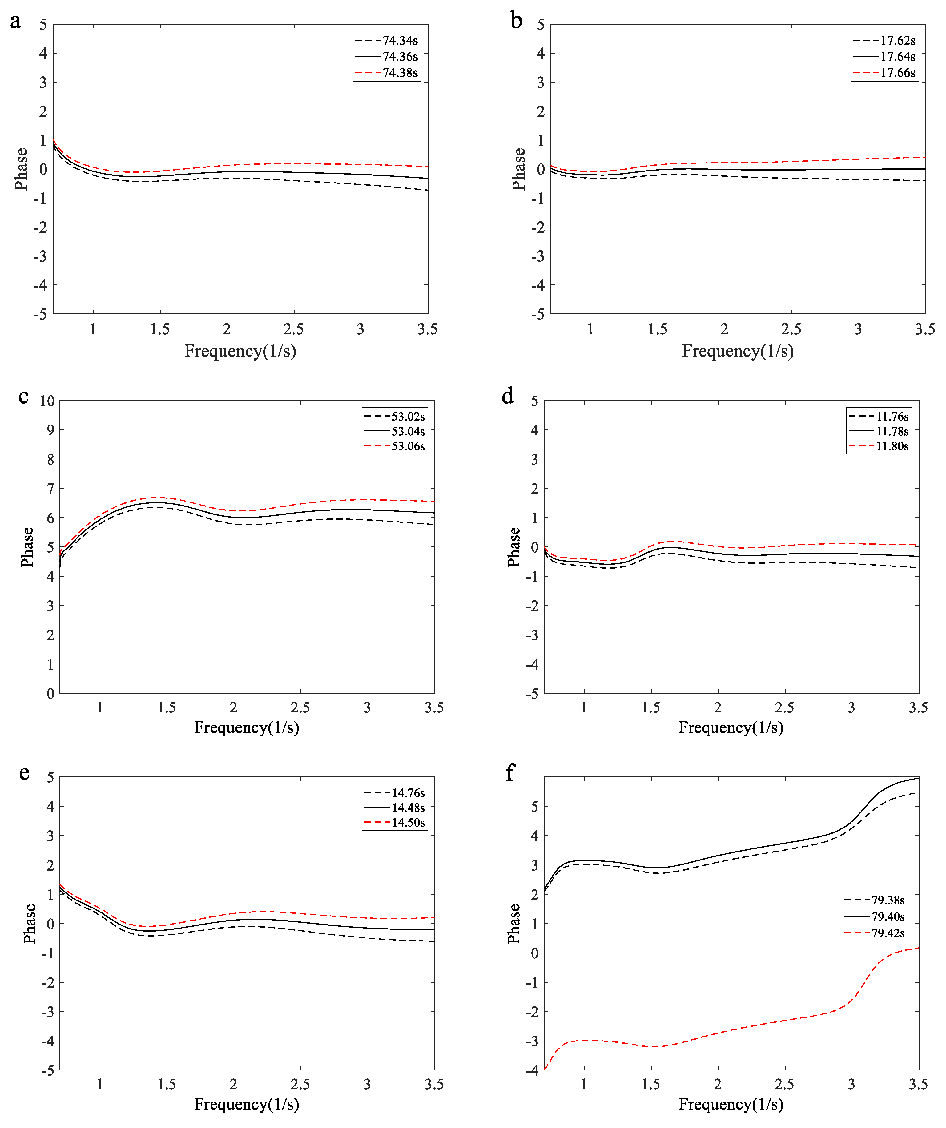
Figure 8.
The variation in wavelet energy spectra during freak-wave evolution under design conditions and .
Figure 8.
The variation in wavelet energy spectra during freak-wave evolution under design conditions and .
4.3. The Wavelet Energy Variation of Freak Waves Evolution Process
In this section, the analysis of wave evolution based on wavelet transform is carried out to further understand the mechanism of freak wave occurrence. Three representative generation processes of freak waves will be analyzed and discussed in detail: freak waves with a single large crest (Type 1) as shown in Figure 5(a)-(b), and “three sisters” freak waves (Type 2) as shown in Figure 5(c).
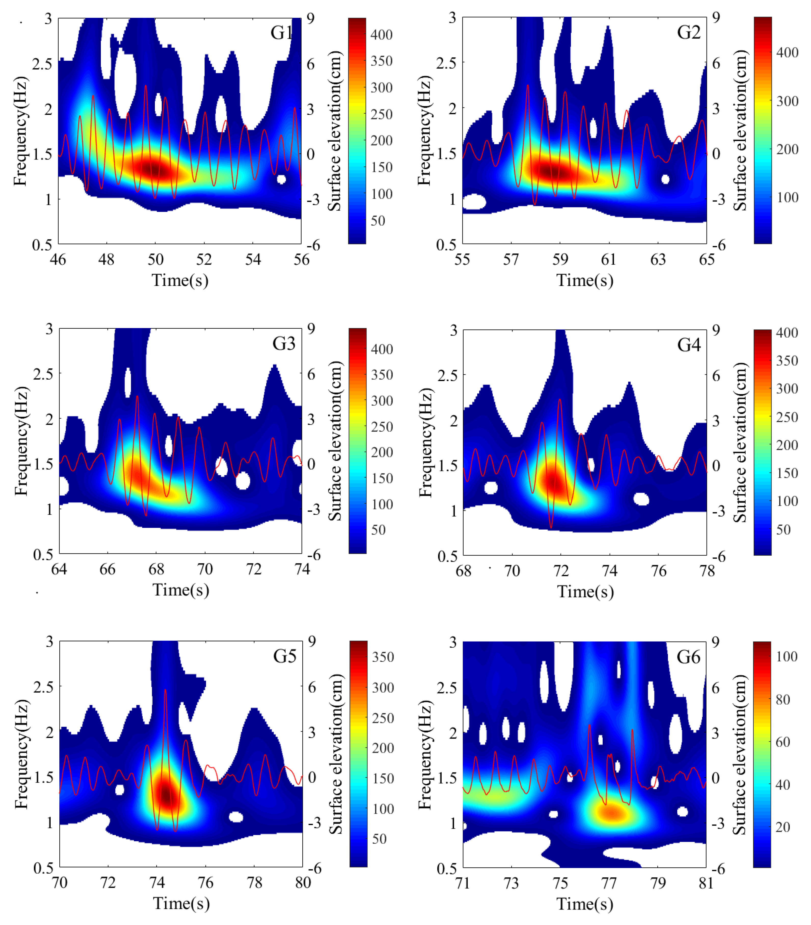
Figure 8 illustrates the generation process of a single crest freak wave shown in Figure 5(a), resulting from a long wave group. This phenomenon is due to wave focusing and merging. A long wave group, emerging between 46s and 55s with smaller wave heights, is depicted in Figure 8(a). The wavelet energy spectrum shows a gradual decrease in wave frequency from 46s to 55s. As the wave group propagates to probe G2, higher-frequency waves at the front merge with lower-frequency waves at the rear. Li et al. also demonstrated that low-frequency components, trailing behind higher-frequency components, merge to form a single crest freak wave [21]. As the wave group propagates, wavelet energy focuses, and wave height increases gradually. The freak wave () appears at probe G5 at 74 seconds, demonstrating a nearly symmetric triangular form in the wavelet energy spectrum. The presence of higher-frequency components indicates stronger nonlinear interactions.
Figure 9 shows another freak wave generation process, originating from several smaller waves within two wave groups, occurring between 3s and 16s. The energy of the first wave group is concentrated in higher frequencies around 1.4Hz-1.7Hz shown in Figure 9(a). The energy distribution of the later wave group forms a “V” pattern, ranging from 0.8Hz to 1.4Hz. The low-frequency wave group catches up with the high-frequency wave group at probe F2. As the waves propagate to probe F3, higher-frequency waves in the latter half of the group lag behind, causing the remaining waves to focus and form a large wave with and at 18s.
Special attention is given to Figure 9(c), where the wavelet energy spectrum differs from that of the freak wave in Figure 8. Here, the energy is not concentrated at a single frequency, and the higher-frequency components exhibit increased energy. Two peak values are observed during the freak crest, consistent with previous observations. As group demodulation occurs, the freak wave completely dissipates at probe F4, with high-frequency energy nearly dissipated, leading to the rapid disappearance of the freak wave.
The formation of larger wave groups may contribute to freak wave events. Figure 10 presents the local wavelet energy spectrum and the evolving wave surface around probes H. The freak wave event depicted in Figure 5(c) is observed at probe H8. In Figure 10(a), a wave group with several large waves occurs between 31s and 37s. The wavelet energy spectrum indicates concentrated wave energy, with the highest value at 1.3 Hz. Higher-frequency components are observed around 33s during the larger waves, but this does not meet the definition of a freak wave.
As the wave group propagates, higher frequency energies are absorbed into lower-frequency components, as illustrated in Figure 10(b). Figure 10(c) shows three consecutive large waves with significant wave height measured between 38s and 40s. Additionally, several smaller waves with higher-frequency energy are located in front of these larger waves. These smaller waves are overtaken by lower-frequency components at probe H4. It is noteworthy that lower-frequency components not only merge with higher-frequency components but also trigger wave interactions, leading to wave group instability. This interaction causes energy transformation from lower to higher frequencies. At probe H5, the wavelet energy spectrum shows concentrated energy, and the number of larger waves decreases from four to three, as shown in Figure 10(e).
A freak wave is observed at probe H6 at 47.5s, with . The wavelet energy trends towards higher frequencies during the occurrence of the freak wave. Upon propagating to probe H7, a wave with a deep trough is measured, with , which meets the definition of freak waves. Additionally, another freak wave, known as the “three sister” freak waves, is observed at probe H8, with . The present results demonstrate that higher-frequency components activate wave group instability, suggesting that the incentive effect of high-frequency components is a significant mechanism in the occurrence of freak waves.
Since the present experiment is based on random waves, it provides strong evidence that the “hole in the sea” phenomenon is an intermediate process in the formation of freak waves. These two freak wave events correspond to cases 15-16 in Table 2, with and This demonstrates that the nonlinearity of repeated freak waves may be stronger, resulting in a larger destructive effect. Continuous freak wave events pose a greater danger to inshore ships, ocean structures, and marine aquaculture, as the probability of encounters will significantly increase.
4.4. Phase Variation Characteristics with Freak Wave Evolution
In section 4.2, the phases based on wavelet transform are investigated during freak crests and troughs according to different waveforms. These findings align with the knowledge provided by Veltcheva and Soares [24]. However, further study on the phases of the freak wave evolution process is needed, primarily because it is challenging to obtain continuous time series of wave surfaces in the open sea. Understanding the phase mechanisms during freak events is crucial. In the current research, the phases of the freak wave evolution process are analyzed in detail, as shown in Figure 11, Figure 12 and Figure 13.
According to the wavelet energy spectrum in Figure 8(a)-(d), the main energy is concentrated in the frequency range of 1~1.7 Hz. The phases in this range remain largely unchanged in Figure 11(a)-(d). Except for Figure 11(c), the phases of higher-frequency components exhibit sharp variations. In Figure 11(e), the appearance of a freak wave is accompanied by consistent phases of higher frequency and main frequency components. Figure 12 shows a similar phenomenon, indicating that the alignment of high-frequency component phases with dominant frequency phases is one reason for freak wave generation. However, there are limitations to this suggestion. For instance, in Figure 11(c), the phase variation is smaller between high and dominant frequencies but larger during lower-frequency components. Additionally, for the freak event in Figure 12, produced from two wave groups, choosing the appropriate crest or trough of the freak-wave source is challenging. These uncertainties can affect the conclusion’s accuracy.
Fortunately, another freak wave evolution process is measured, as shown in Figure 13, compensating for the aforementioned defects. The phases of the dominant frequency range from 1 to 1.8 Hz exhibit narrow fluctuations. In contrast, the phases of higher-frequency components differ significantly from those of the dominant frequency components. When the large crest of a freak wave is generated, the phases tend to become uniform, as shown in Figure 13(f) and (h). Even during the freak trough, the same result is observed across a wide range of frequencies up to 3 Hz. These data lead us to the definitive conclusion that the alignment of higher-frequency component phases with those of the dominant frequency components is a critical mechanism in the generation of freak waves.
4.5. Nonlinear Interactions with Freak Wave Evolution
Freak wave events are usually accompanied by strong nonlinearity. The wavelet-based cross-bispectrum is an effective tool for analyzing nonlinear phase coupling related to nonlinear wave-wave interactions [26,28]. In the current study, summed bicoherence and total bicoherence are calculated using Eqs. (21)-(22). The total bicoherence of wave groups, which are the sources of freak wave events, is shown in Figure 14. Freak waves are detected at probes G5, F3, and H6-H8, corresponding to the freak wave evolution shown in Figure 8, Figure 9 and Figure 10. It is observed that the maximum total bicoherence accompanies the occurrence of large freak crests, indicating a stronger degree of quadratic nonlinear interactions in freak waves. The corresponding summed bicoherence is shown in Figure 15. It demonstrates that the nonlinear interaction of higher-frequency components significantly increases during freak wave occurrences, suggesting that higher-frequency components also play a crucial role in nonlinear interactions.
Figure 16 presents the results for freak wave groups and the continuous time series of their evolution surface over time, based on Equation (26). In Figure 16(a), it is illustrated that the parameter tends to decrease gradually from the front to the back of the wave group at probe G1 (black curve). As the wave group propagates, it is evident that wave components with higher values will follow those with lower values. The parameter is significantly large at the freak crest when it occurs at probe G5. When the wave group propagates from probe G4 to G5, the parameter increases by 0.33 Hz, as determined by subtracting the largest value at probe G4 (pink curve) from that at probe G5 (green curve). This method quantitatively analyzes the degree of energy transfer during freak wave generation.
The advantage of is that it allows the weighted mean of the wavelet energy spectrum to be obtained at each sample time, enabling detailed analysis of the energy transfer during freak wave generation. Figure 16 shows the results of ABC for freak wave groups and the continuous time series of their evolving surface over time span , based on Eq. (26). In Figure 16(a), it is shown that tends to decrease gradually from the front to the back of the wave group at probe G1 (black curve). As the wave group propagates, the wave components with larger values follow those with lower values. The value is notably high at the freak crest observed at probe G5. When the wave group moves from probe G4 to G5, increases by 0.33Hz, calculated by subtracting the highest value at probe G4 (pink curve) from that at probe G5 (green curve). This method allows for a quantitative analysis of the energy transfer degree during freak wave generation. In Figure 16(b), it is demonstrated that shifts towards higher frequencies at probe F3, where a freak wave is observed. Furthermore, increases by 0.06Hz and 0.17Hz at probes H6 and H8, respectively, as shown in Figure 16(d). These results confirm that is a reliable indicator of energy transfer.
Previously, we analyzed that high-frequency small waves induce wave group instability based on the wavelet energy spectrum, leading to wave energy concentration. This phenomenon is clearly identified through in Figure 16(c), which shows an increase in in the first half of the wave group at probe H4. Its trend along the wave group is similar to the results at probe G1 in Figure 16(a), gradually evolving into a freak wave event as the wave group propagates.
4. Conclusions
In this paper, freak waves are observed and studied in random waves within a wave tank as they pass over a 3-D reef terrain model, measured in the western Pacific. Twenty-one freak wave events were recorded in a recent experiment and can be classified into four types: a huge single crest, a freak group, a vertically symmetrical freak wave, and a “hole in the sea.” These types are also the main categories of freak wave events in the actual ocean, demonstrating the effectiveness of the current experiment for freak wave research using measured topographic data from the open sea in random waves.
The wavelet transform method is used to analyze the characteristics and mechanisms of freak wave occurrences, including the wavelet energy spectrum, scale-averaged wavelet power , time-averaged wavelet spectrum , local values, phases of wavelet transform, and wave-wave nonlinear interactions based on wavelet cross-bispectrum. The results indicate that both linear superposition with coherent phase and wave-wave nonlinear interaction contribute to freak wave events. The wavelet energy spectrum shows that low-frequency energy transforms into high-frequency energy during the generation of freak waves. A new parameter, the scale-centroid wavelet spectrum, is defined based on the wavelet transform algorithm to quantitatively analyze the extent of energy transfer. It shows that the parameter is an effective indicator of interscale energy transfer during freak-wave events. The phases of higher-frequency components progressively align with those of the dominant band, leading to the freak-wave event. Linear superposition influences the evolution well before the rogue wave forms, whereas nonlinear interactions intensify only in the short interval immediately preceding its onset. Meanwhile, wavelet cross-bispectrum estimates further indicate that wave-wave coupling is strongest in the high-frequency band.
This study investigates the evolution of freak waves, identifies the causes of their generation over three-dimensional bathymetry, elucidates the roles of linear superposition and nonlinear interactions in their occurrence, provides important evidence for the underlying mechanisms, and offers guidance for forecasting.
Author Contributions
Wang Aimin; writing—original draft preparation, Zhou Tao; data curation, Ding Dietao; investigation, Ma Xinyu; writing—review and editing, Zou Li; supervision. All authors have read and agreed to the published version of the manuscript.
Funding
The present work is supported by, Natural Science Foundation of Jiangsu Province of China (No.BK20230668), the PI Project of Southern Marine Science and Engineering Guangdong Laboratory (Guangzhou) (GML20240001, GML2024009).
References
- Dean, R. G. Freak waves: a possible explanation. In Water wave kinematics. Springer Netherlands, 1990; pp. 609-612.
- Soares, C. G., Cherneva, Z., & Antão, E. M. Characteristics of abnormal waves in North Sea storm sea states. Applied Ocean Research, 2003; 25(6), 337-344. [CrossRef]
- Kharif, C., Pelinovsky, E., & Slunyaev, A. Rogue Waves in the Ocean, 2009; Springer Berlin Heidelberg.
- Xue, S. Xu, G., Xie, W., et al. Characteristics of freak wave and its interaction with marine structures: a review. Ocean engineering, 2023 ;(Nov.1 Pt.1), 287.
- Acanfora, M., Coppola, T., Fasano, E.. Estimation of rogue wave loads on ship structures by exploiting linear wave theory[M]. Developments in the Analysis and Design of Marine Structures. CRC Press, 2021; pp.3-9.
- Luo, M., Koh, C. G., Lee, W. X., et al. Experimental study of freak wave impacts on a tension-leg platform[J]. Marine Structures, 2020; 74: 102821. [CrossRef]
- Liu, B., Yu, J. Dynamic response and mooring fracture performance analysis of a semi-submersible floating offshore wind turbine under freak waves. Journal of Marine Science and Engineering, 2024; 12. [CrossRef]
- Pan, W., He, M., & Cui, C. Experimental Study on Hydrodynamic Characteristics of a Submerged Floating Tunnel under Freak Waves (I: Time-Domain Study). Journal of Marine Science and Engineering, 2023; 11(5), 977. [CrossRef]
- Lawton, G. Monsters of the deep. New Scientist, 2001; 170(2297), 28-32.
- Haver, S. A possible freak wave event measured at the Draupner jacket January 1 1995. Rogue waves 2004, 2004; 1-8.
- Veltcheva, A. D., & Soares, C. G. Analysis of abnormal wave groups in Hurricane Camille by the Hilbert Huang Transform method. Ocean Engineering,2012; 42, 102-111. [CrossRef]
- Cherneva, Z., & Soares, C. G. Time–frequency analysis of the sea state with the Andrea freak wave. Natural Hazards and Earth System Sciences, 2014; 14(12), 3143-3150. [CrossRef]
- Didenkulova, E., Didenkulova, I., & Medvedev, I. Freak wave events in 2005-2021: statistics and analysis of favourable wave and wind conditions. Natural Hazards & Earth System Sciences Discussions, 2023; 23, 1653–1663. [CrossRef]
- Bitner-Gregersen, E. M., Gramstad, O., et al. Rogue waves: results of the exwamar project. Ocean engineering, 2024; Jan.15, 292. [CrossRef]
- Mori, N., Waseda, T. and Chabchoub, A., eds.. Science and Engineering of Freak Waves. Elsevier, 2023,pp.1:55.
- Onorato, M., Osborne, A. R., Serio, M. et al. Extreme waves, modulational instability and second order theory: wave flume experiments on irregular waves. European Journal of Mechanics-B/Fluids, 2006; 25(5), 586-601. [CrossRef]
- Li, J., Li, P., & Liu, S. Observations of freak waves in random wave field in 2D experimental wave flume. China Ocean Engineering, 2013; 27, 659-670. [CrossRef]
- Toffoli, A., Waseda, T., Houtani, H., et al. Rogue waves in opposing currents: an experimental study on deterministic and stochastic wave trains. Journal of Fluid Mechanics, 2015; 769, 277-297. [CrossRef]
- Zhang, H. D., Wang, X. J., Shi, H. D., et al. Investigation on abnormal wave dynamics in regular and irregular sea states. Ocean Engineering, 2021; 222, p.108602. [CrossRef]
- Chabchoub, A. Tracking breather dynamics in irregular sea state conditions[J]. Physical Review Letters, 2016; 117(14): 144103. [CrossRef]
- Li, J., Yang, J., Liu, S., Ji, X. Wave groupiness analysis of the process of 2D freak wave generation in random wave trains[J]. Ocean Engineering, 2015; 104, 480-488. [CrossRef]
- Lee, B. C., Kao, C. C., Doong, D. J. An analysis of the characteristics of freak waves using the wavelet transform[J]. Terr. Atmos. Ocean. Sci., 2011; 22, 359-370. [CrossRef]
- Christou, M., and Ewans, K. Field measurements of rogue water waves[J]. Journal of Physical Oceanography, 2014; 44(9), pp.2317-2335. [CrossRef]
- Veltcheva, A., Soares, C. G. Wavelet analysis of non-stationary sea waves during Hurricane Camille[J]. Ocean Engineering, 2015; 95: 166-174. [CrossRef]
- Slunyaev, A., Pelinovsky, E., Soares, C. G. Modeling freak waves from the North Sea[J]. Applied Ocean Research, 2005; 27(1): 12-22. [CrossRef]
- Dong, G., Ma, Y., Perlin, M., et al. Experimental study of wave–wave nonlinear interactions using the wavelet-based bicoherence. Coastal Engineering, 2008; 55(9), 741-752. [CrossRef]
- Zhang, S., Lian, J., Li, J., et al. Wavelet bispectral analysis and nonlinear characteristics in waves generated by submerged jets. Ocean Engineering, 2022; 264, 112473. [CrossRef]
- Ma, Y., Tai, B., Dong, G., Fu, R., et al. An experiment on reconstruction and analyses of in-situ measured freak waves. Ocean Engineering, 2022; 244, 110312. [CrossRef]
- Deng, Y., Yang, J., Tian, X., et al. An experimental study on deterministic freak waves: Generation, propagation and local energy. Ocean Engineering, 2016; 118, 83-92. [CrossRef]
- Christou, M., Ewans, K., Buchner, B., et al. Spectral characteristics of an extreme crest measured in a laboratory basin[C]. Proc. Rogue Waves, 2008; 165-178.
- Fedele, F., Brennan, J., SPD, L., et al. Real world ocean rogue waves explained without the modulational instability. Scientific Reports, 2016; 6(1): 1-1. [CrossRef]
- Ji, X., Li, A., Li, J., et al. Research on the statistical characteristic of freak waves based on observed wave data. Ocean Engineering, 2022; 243, p.110323. [CrossRef]
- Janssen, T. T., Herbers, T. H. C. Nonlinear wave statistics in a focal zone[J]. Journal of Physical Oceanography, 2009; 39(8): 1948-1964. [CrossRef]
- Zhang, J., Benoit, M. Wave–bottom interaction and extreme wave statistics due to shoaling and de-shoaling of irregular long-crested wave trains over steep seabed changes[J]. Journal of Fluid Mechanics, 2021, 912. [CrossRef]
- Trulsen, K., Zeng, H., Gramstad, O. Laboratory evidence of freak waves provoked by non-uniform bathymetry[J]. Physics of Fluids, 2012; 24(9): 740-310. [CrossRef]
- Trulsen, K., Raustøl, A., Jorde, S., et al. Extreme wave statistics of long-crested irregular waves over a shoal[J]. Journal of Fluid Mechanics, 2020; 882. [CrossRef]
- He, Y., Chen, H., Yang, H., et al. Experimental investigation on the hydrodynamic characteristics of extreme wave groups over unidirectional sloping bathymetry. Ocean Engineering, 2023; 282, p.114982. [CrossRef]
- Toffoli, A., Cavaleri, L., Babanin, A. V., et al. Occurrence of extreme waves in three-dimensional mechanically generated wave fields propagating over an oblique current. Natural Hazards and Earth System Sciences, 2011; 11(3), 895-903. [CrossRef]
- Toffoli, A., Proment, D., Salman, H., et al. Wind generated rogue waves in an annular wave flume. Physical review letters, 2017; 118(14), 144503. [CrossRef]
- Benjamin, T. B., & Feir, J. E. The disintegration of wave trains on deep water Part 1. Theory. Journal of Fluid Mechanics, 1967; 27(03), 417-430. [CrossRef]
- Xie, S., Tao, A., Fan, J., et al. Long time evolution of modulated wave trains. Ocean Engineering, 2024; 311(Part1), 17. [CrossRef]
- Dysthe, K., Krogstad, H. E., & Müller, P. Oceanic rogue waves. Annu. Rev. Fluid Mech., 2008; 40, 287-310. [CrossRef]
- Slunyaev, A., Didenkulova, I., & Pelinovsky, E. Rogue waters. Contemporary physics, 2011; 52(6), 571-590. [CrossRef]
- Chabchoub, A., Onorato, M., Akhmediev, N. Hydrodynamic envelope solitons and breathers. Rogue and Shock Waves in Nonlinear Dispersive Media. Springer, Cham., 2016; 55-87.
- Goda, Y. A comparative review on the functional forms of directional wave spectrum. Coastal Engineering Journal, 1999; 41(1), 1-20. [CrossRef]
- Zhuang, Y., Wang, Y., Shen, Z., et al. Analysis of statistical characteristics of freak waves based on high order spectral coupled with cfd method. Ocean Engineering, 2025; 323(000). [CrossRef]
- Torrence, C., & Compo, G. P. A practical guide to wavelet analysis. Bulletin of the American Meteorological society, 1998; 79(1), 61-78.
- Glejin J, Kumar V S, Nair T M B, et al. Freak waves off Ratnagiri, west coast of India. Indian Journal of Geo-Marine Sciences, 2014; 43(7):1-7.
Figure 1.
Setup of model in current experiment.
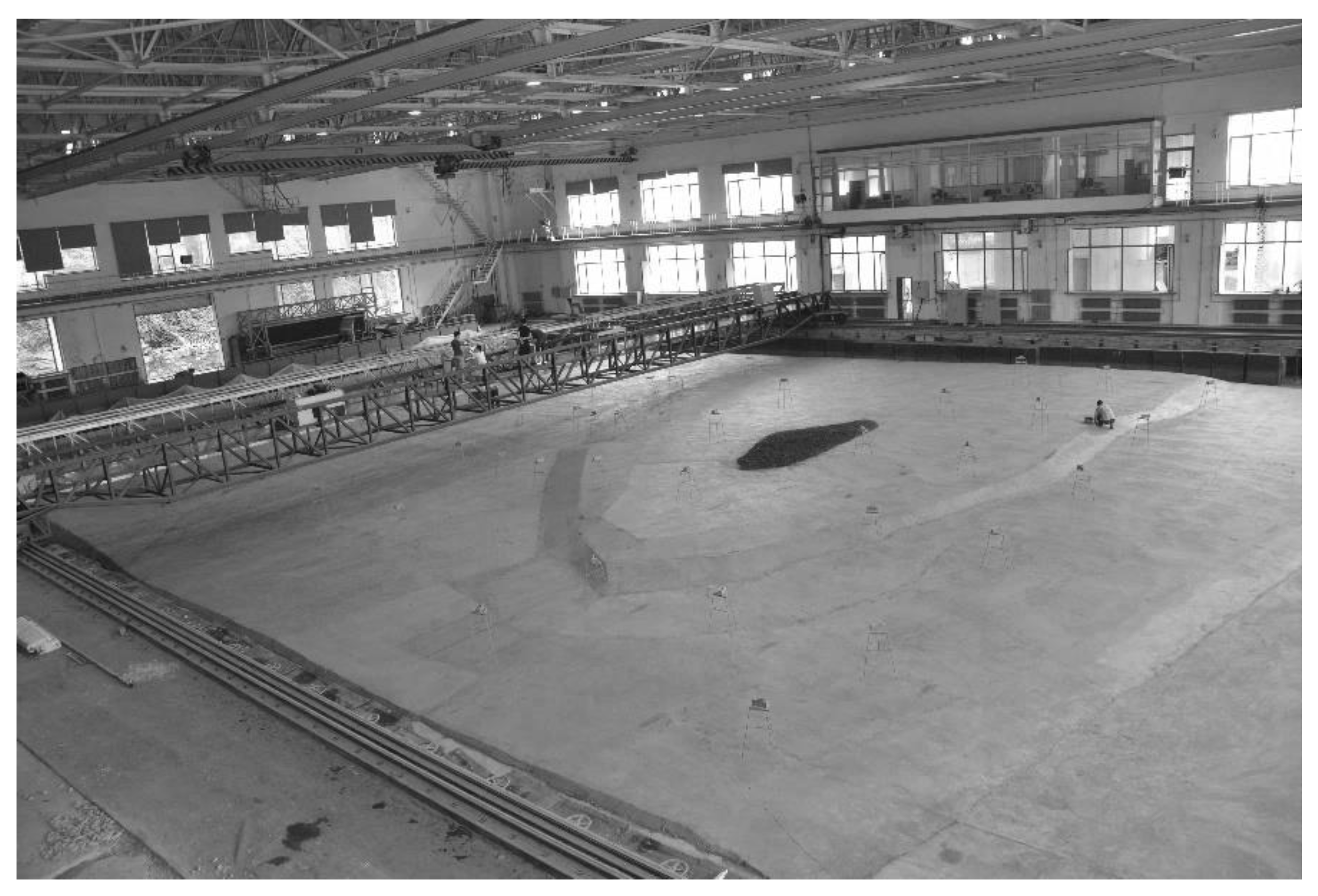
Figure 2.
The natural island located in the western pacific.
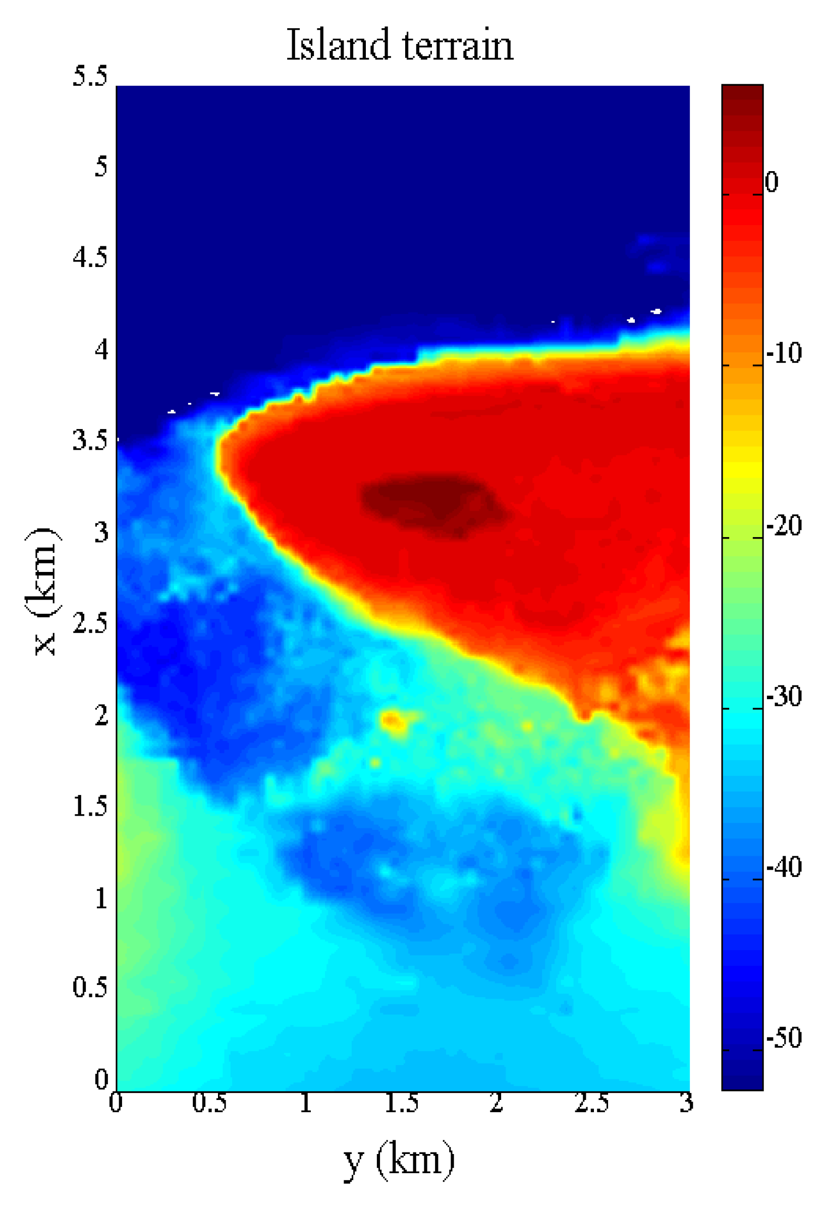
Figure 3.
The arrangement of wave probes.
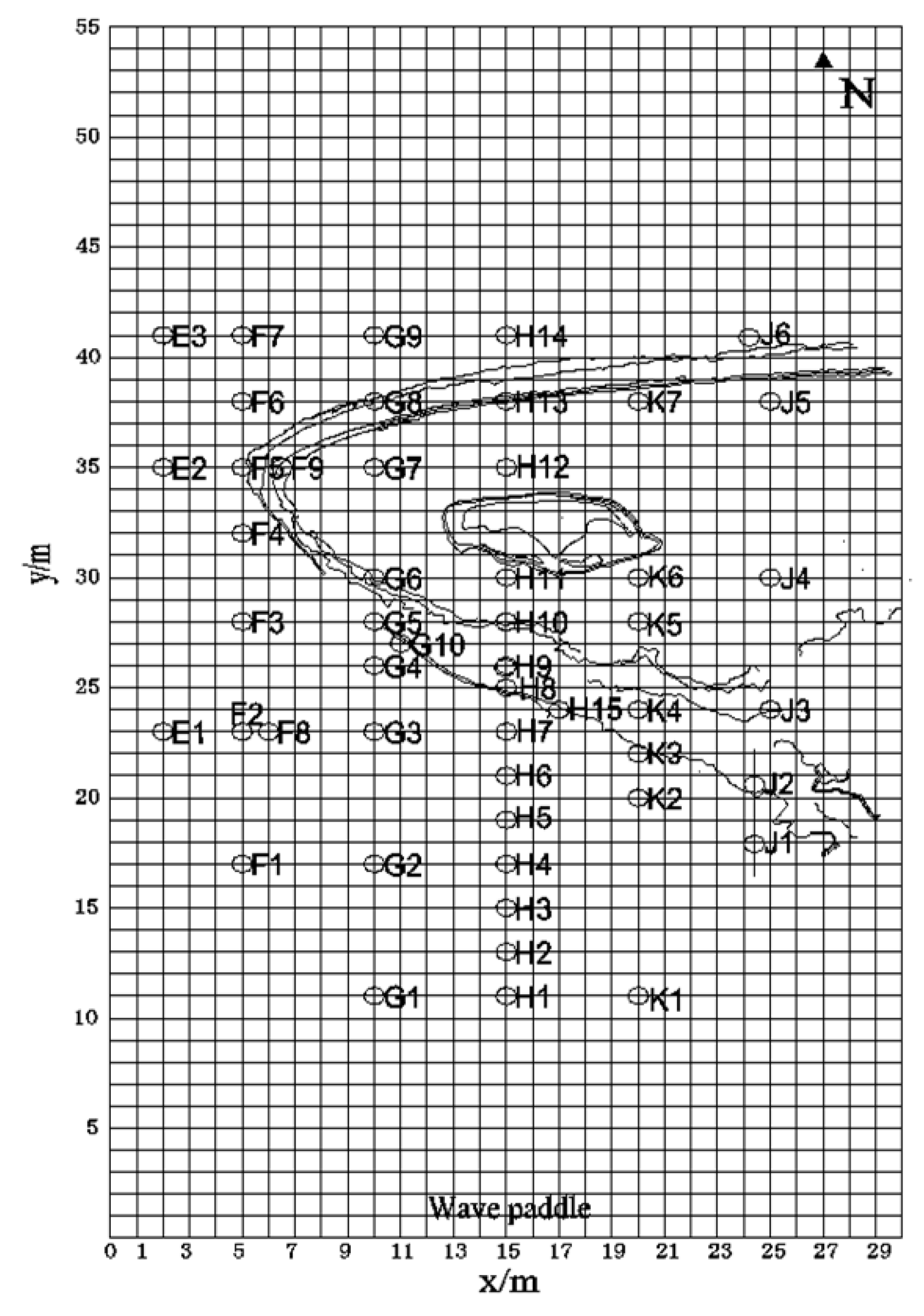
Figure 4.
The wavelet transform for case 2 in Table 2, where , . (a) The wave time series in the experiment (red solid line) and its wavelet energy spectrum; (b) the global wavelet spectrum (solid line) and the time-averaged wavelet spectrum over a certain period (dash line); (c) the scale-averaged wavelet power and its mean value (read line).
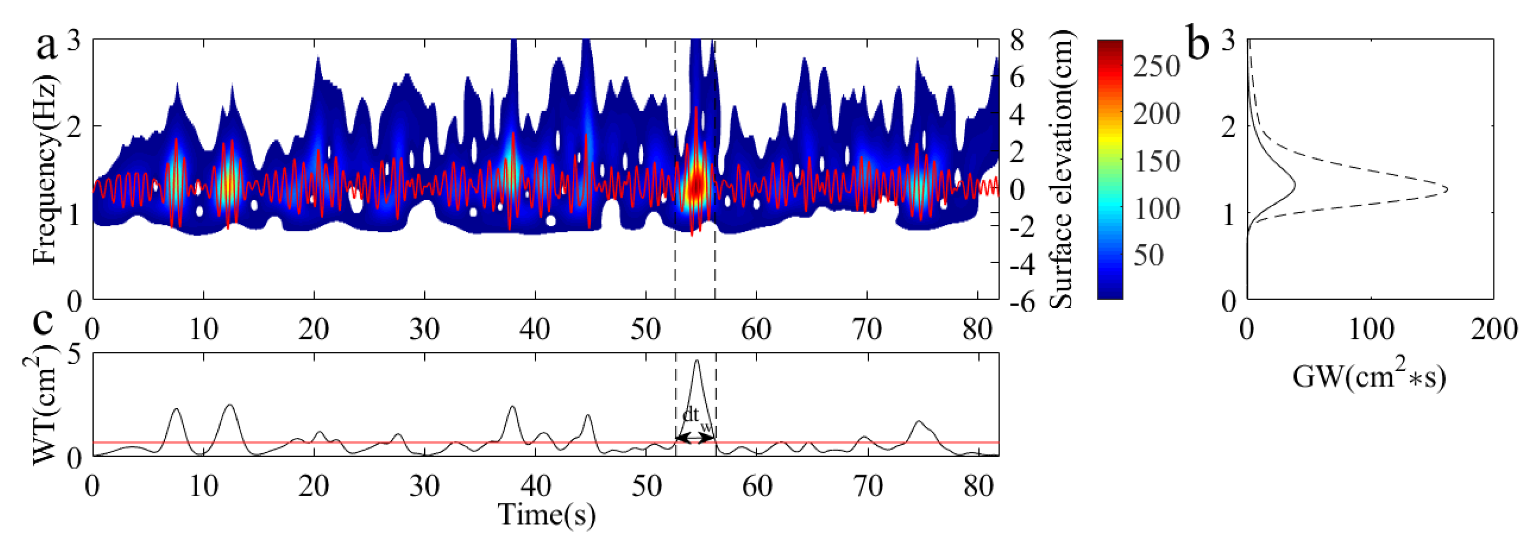
Figure 5.
Different types of freak-wave time series in the experiment. (a) and (b) Huge single crest; (c) Freak wave group; (d) Freak wave group in shallow water; (e) Vertically symmetrical freak wave; (f) “Hole in the sea”.
Figure 5.
Different types of freak-wave time series in the experiment. (a) and (b) Huge single crest; (c) Freak wave group; (d) Freak wave group in shallow water; (e) Vertically symmetrical freak wave; (f) “Hole in the sea”.
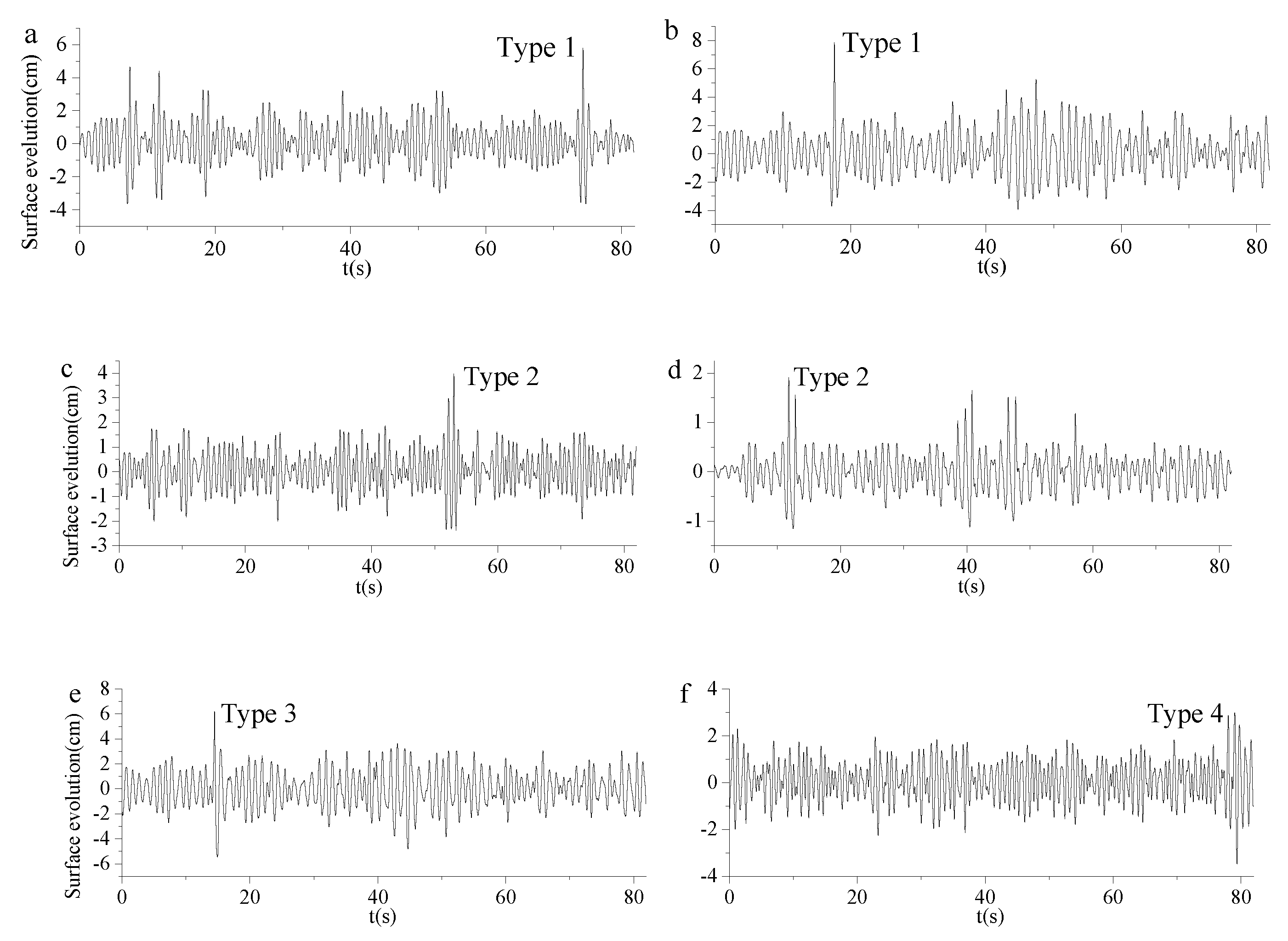
Figure 6.
Time series of wave surface and its wavelet transform results corresponding to freak waves shown in Figure 5.
Figure 6.
Time series of wave surface and its wavelet transform results corresponding to freak waves shown in Figure 5.
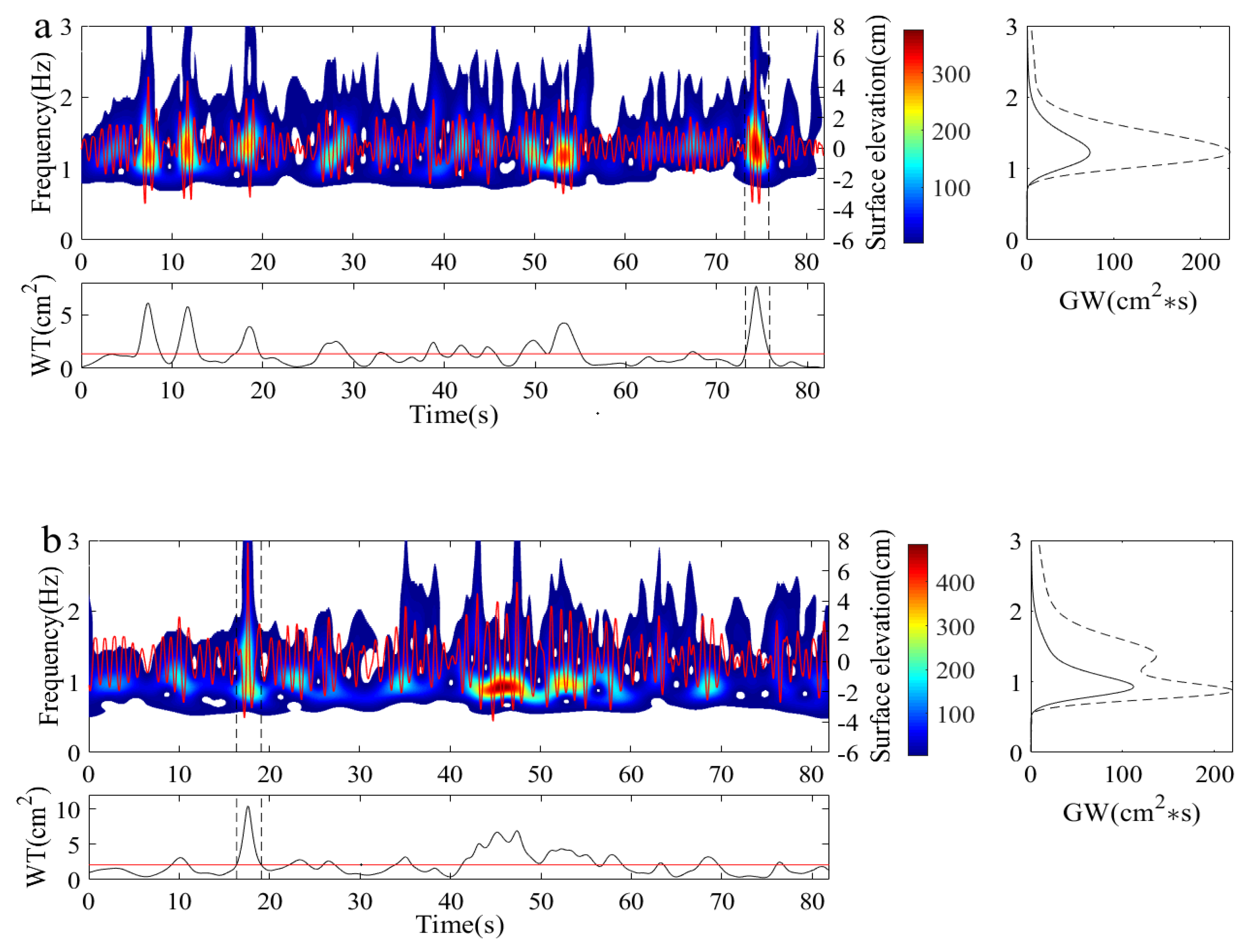
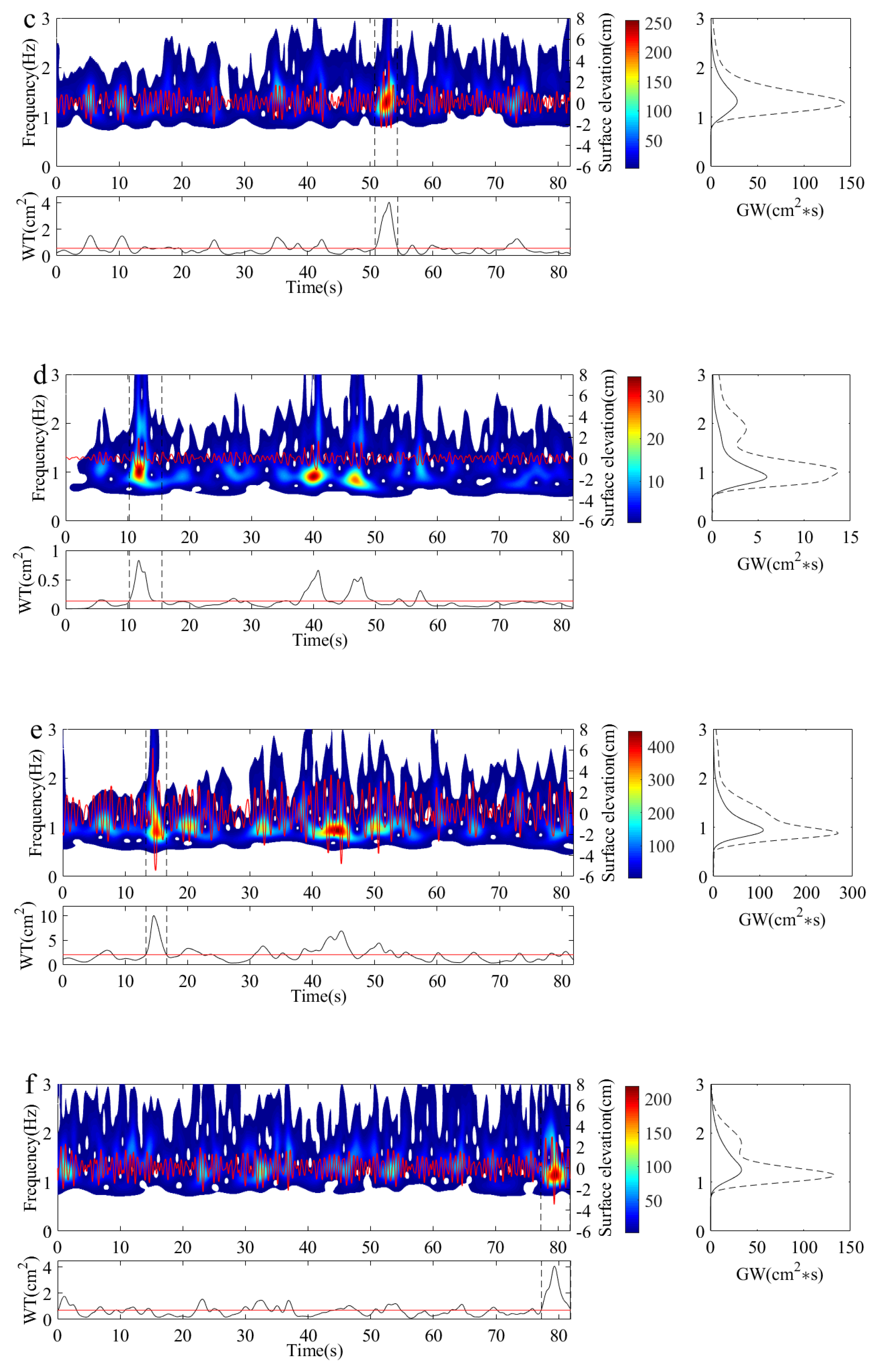
Figure 9.
The variation in wavelet energy spectra during freak-wave evolution under design conditions and .
Figure 9.
The variation in wavelet energy spectra during freak-wave evolution under design conditions and .
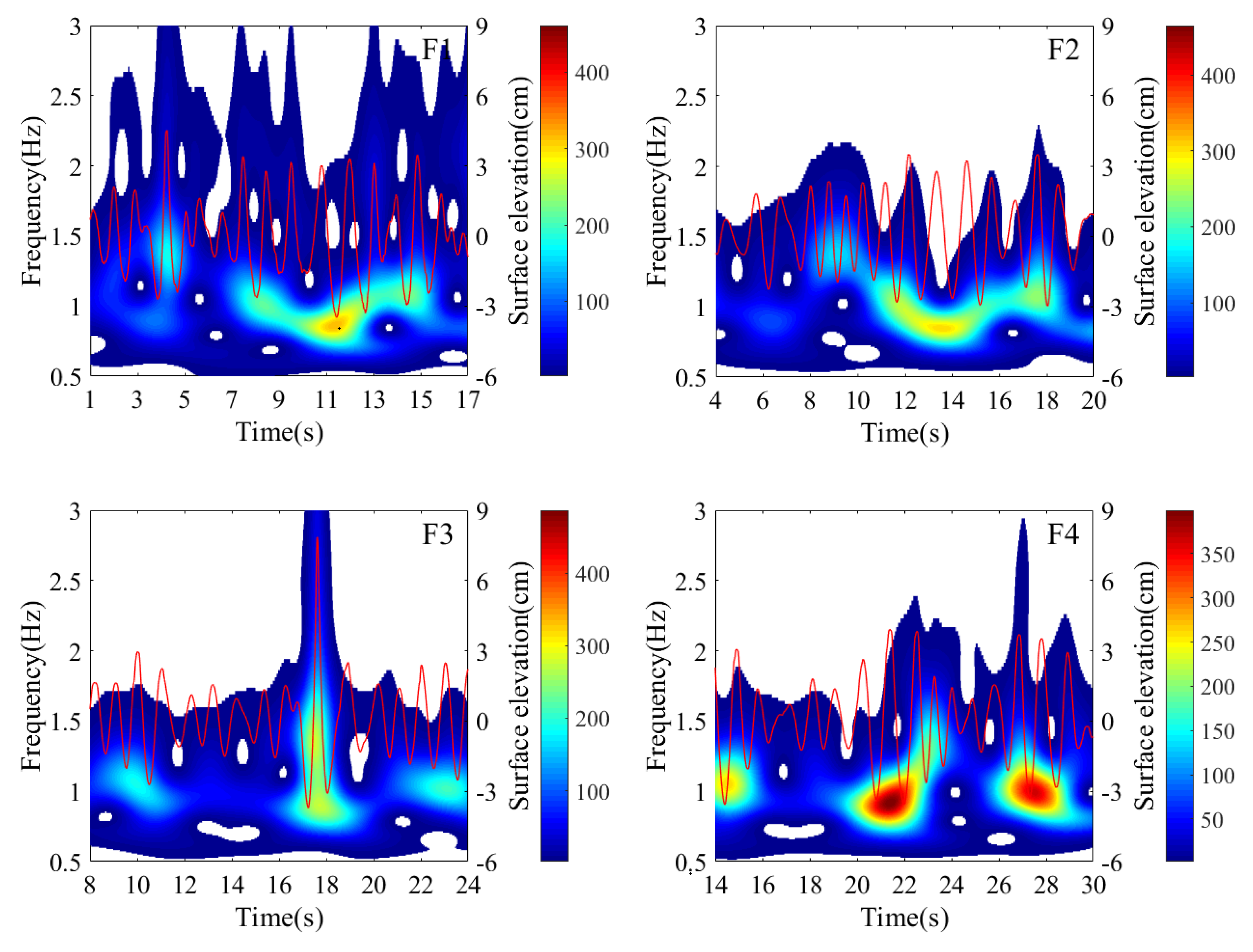
Figure 10.
The variation in wavelet energy spectra during freak-wave evolution under design conditions and .
Figure 10.
The variation in wavelet energy spectra during freak-wave evolution under design conditions and .
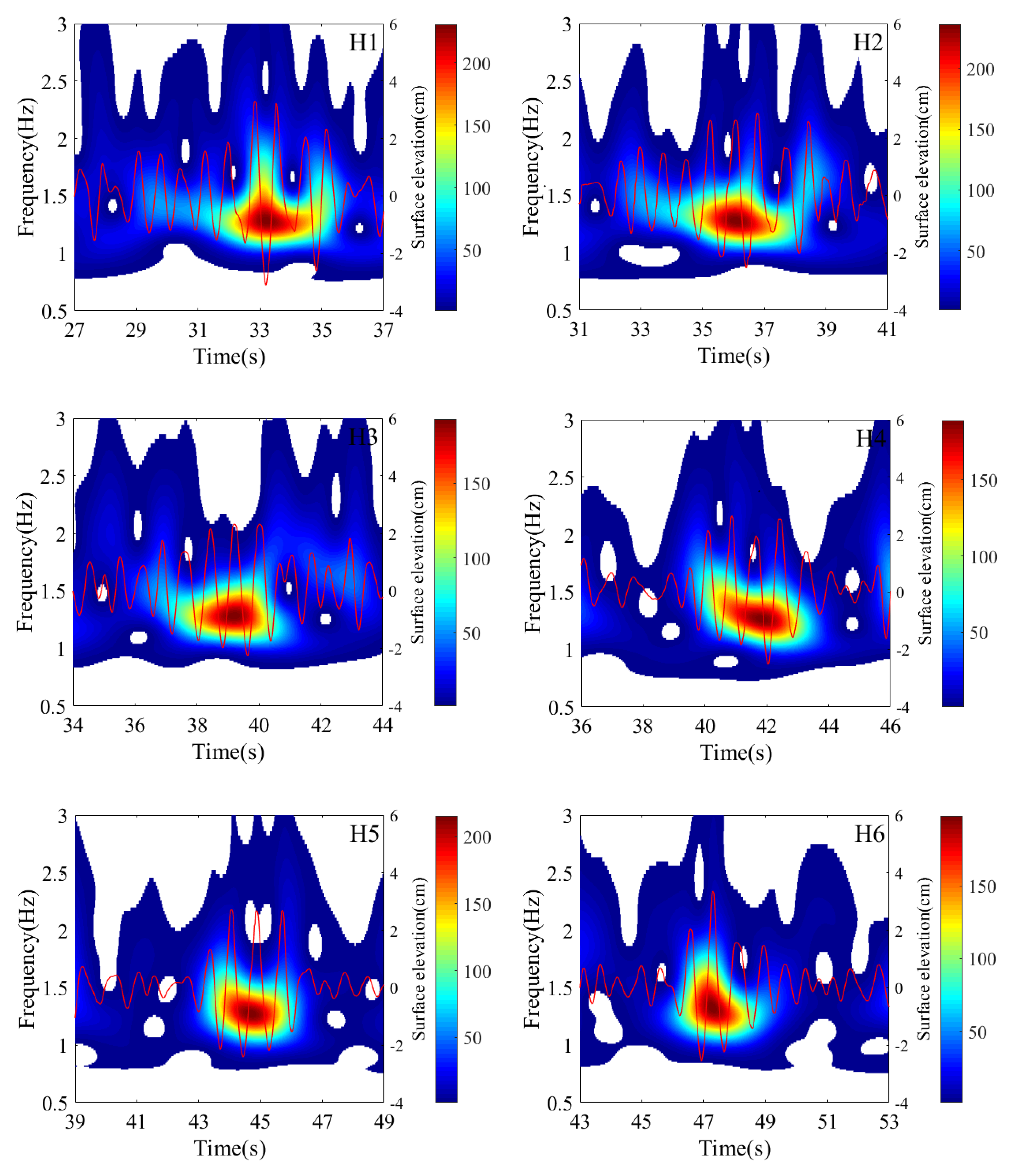
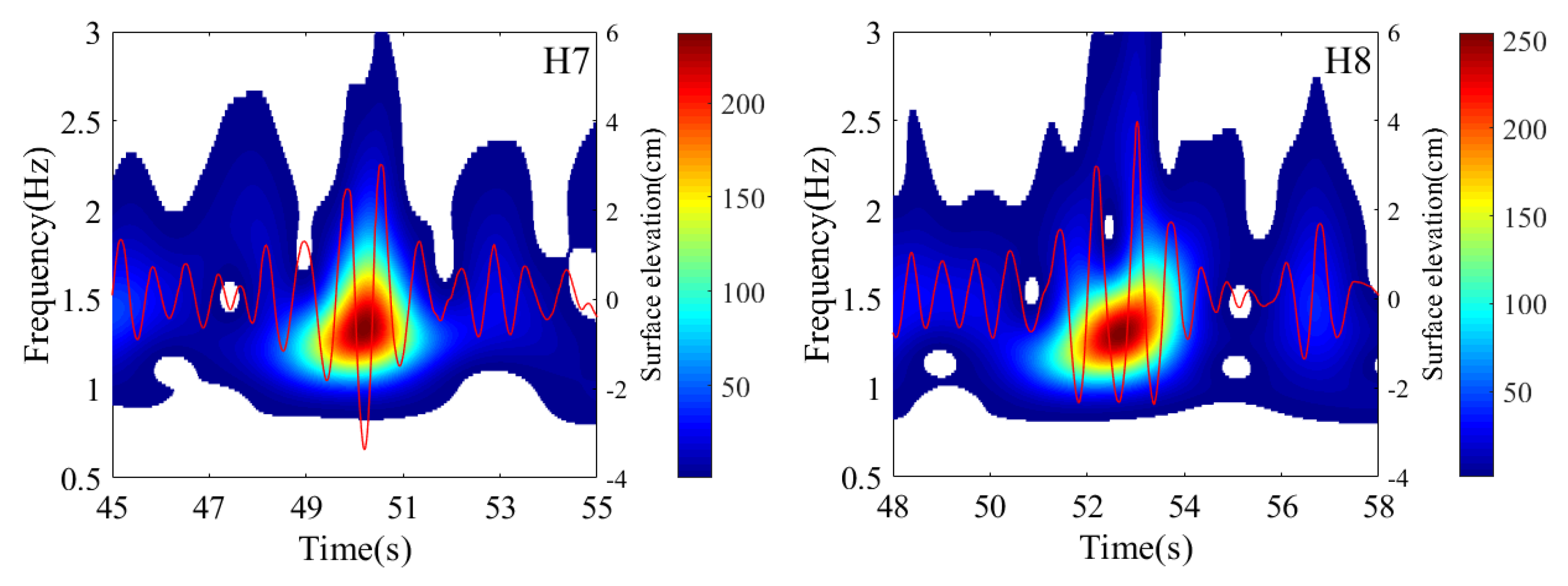
Figure 11.
The phases of wavelet components as function of frequency during freak wave evolution in Figure 8.
Figure 11.
The phases of wavelet components as function of frequency during freak wave evolution in Figure 8.
Figure 12.
The phases of wavelet components as function of frequency during freak wave evolution in Figure 9.
Figure 12.
The phases of wavelet components as function of frequency during freak wave evolution in Figure 9.
Figure 13.
The phases of wavelet components as function of frequency during freak wave evolution in Figure 10.
Figure 13.
The phases of wavelet components as function of frequency during freak wave evolution in Figure 10.
Figure 14.
The total bicoherence corresponding to freak wave evolution shown in Figure 8, Figure 9 and Figure 10. Freak wave occurs at (a) probe G5, (b) probe F3, (c) probes H6-H8.
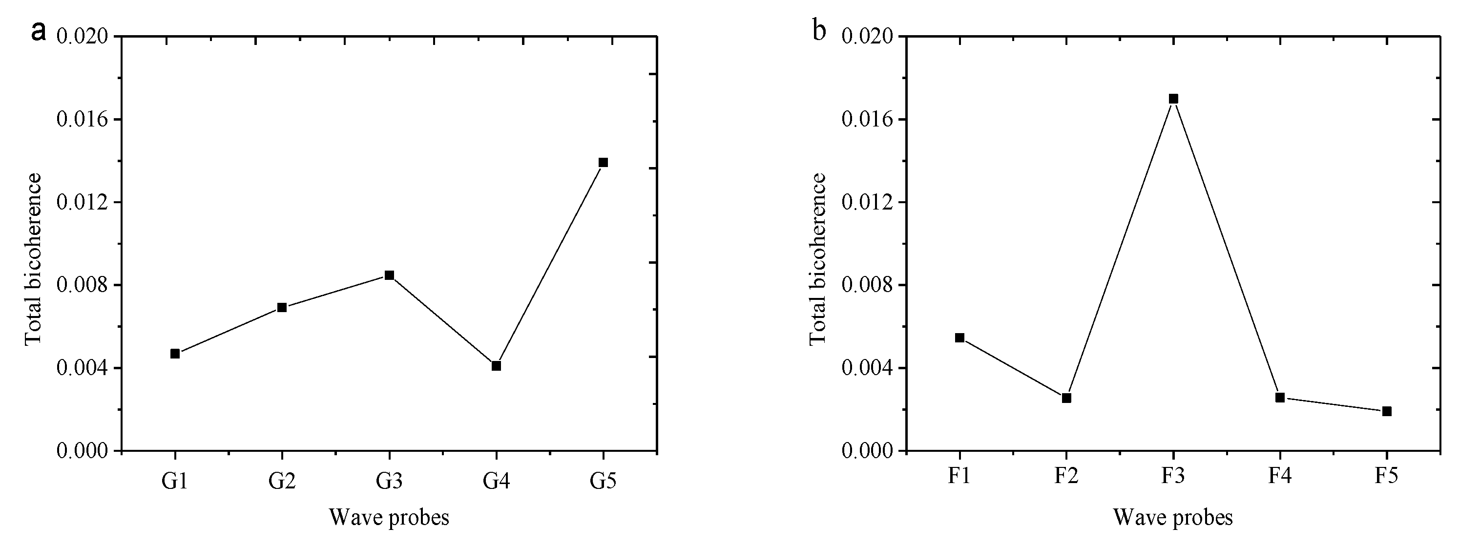
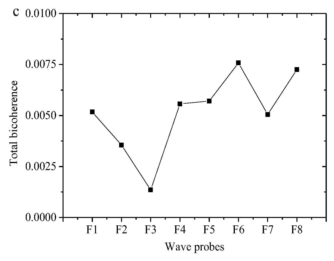
Figure 15.
The summed bicoherence corresponding to freak wave evolution shown in Figure 8, Figure 9 and Figure 10. Freak wave occurs at (a) probe G5, (b) probe F3, (c) probes H6-H8.
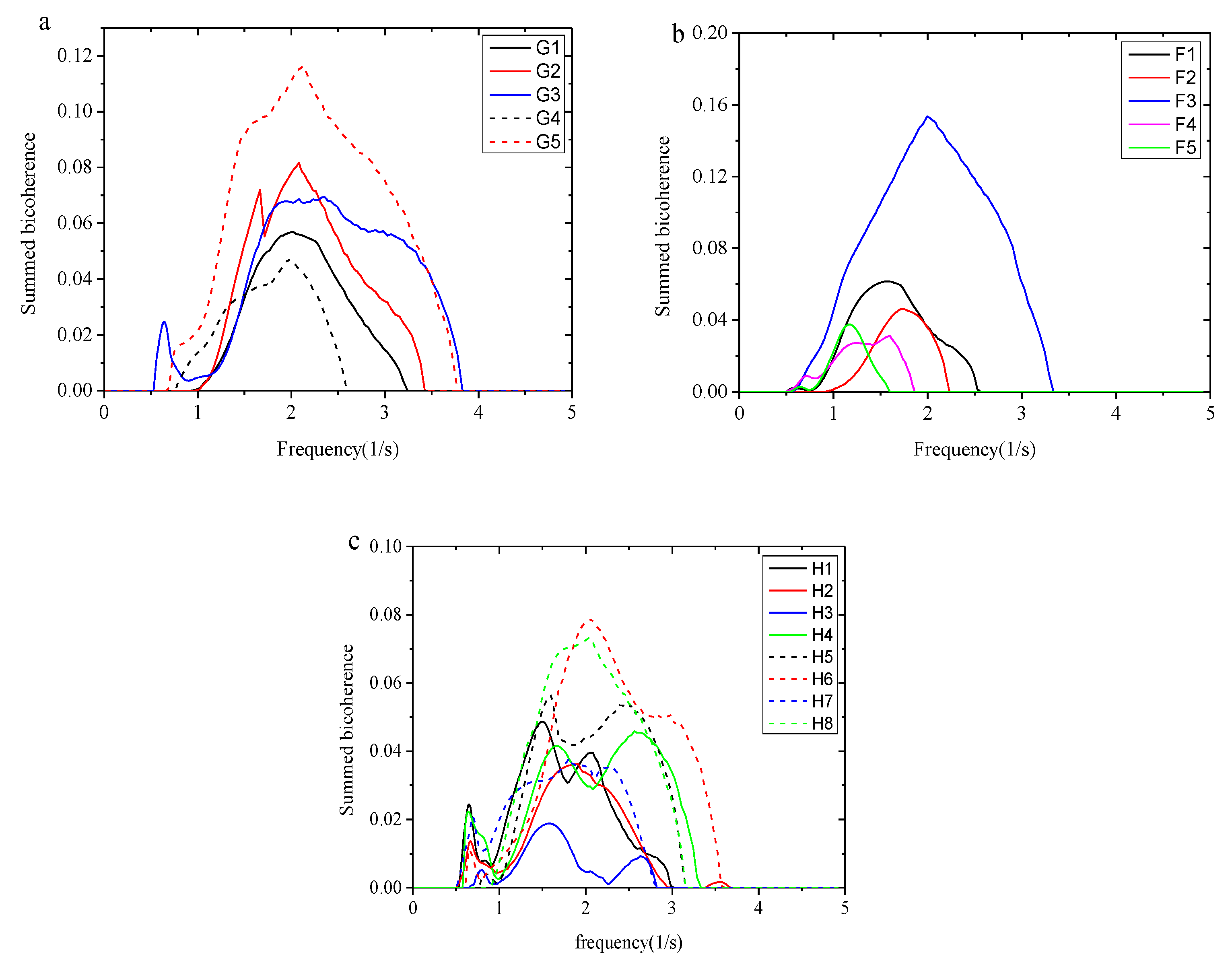
Figure 16.
The scale-centroid wavelet spectrum variation of wave group in time span . (a) The corresponds to Figure 8; (b) The corresponds to Figure 9; (c) The corresponds to Figure 10 at probes H1-H4; (d) The corresponds to Figure 10 at probes H5-H8.
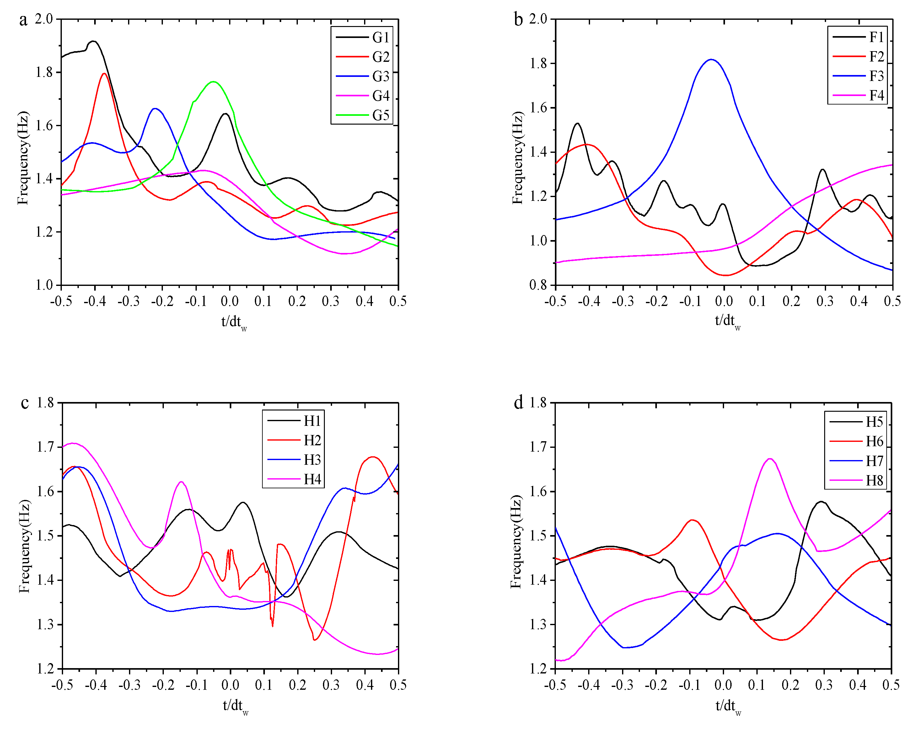

Table 1.
wave parameters of 30 cases in terms of significant wave height and significant period .
| Case | /cm | /s |
|---|---|---|
| A1 | 1.61 | 0.67、0.73、0.8、0.87、0.93、1、1.07、1.21 |
| A2 | 3.59 | 0.67、0.73、0.8、0.87、0.93、1、1.07、1.14 |
| A3 | 6.35 | 0.8、0.87、0.93、1、1.07、1.14、1.21 |
| A4 | 8.05 | 0.8、0.87、0.93、1、1.07、1.14、1.21 |
Table 2.
The parameters of twenty-one freak wave events in experiment.
| Case | Hfr/Hs | Hcr/Hs | Hcr/Hfr | Tfr | Ts | Type | Names |
|---|---|---|---|---|---|---|---|
| 1 | 2.40 | 1.53 | 0.64 | 0.56 | 0.62 | Type 1 | Huge single crest |
| 2 | 2.28 | 1.45 | 0.63 | 0.70 | 0.77 | ||
| 3 | 2.01 | 1.17 | 0.58 | 0.82 | 0.74 | ||
| 4 | 2.08 | 1.31 | 0.63 | 0.74 | 0.79 | ||
| 5 | 2.01 | 1.20 | 0.60 | 0.58 | 0.67 | ||
| 6 | 2.16 | 1.28 | 0.59 | 0.64 | 0.68 | ||
| 7 | 2.07 | 1.27 | 0.61 | 0.74 | 0.78 | ||
| 8 | 2.10 | 1.23 | 0.59 | 0.92 | 0.79 | ||
| 9 | 2.03 | 1.25 | 0.61 | 0.74 | 0.85 | ||
| 10 | 2.04 | 1.32 | 0.65 | 0.74 | 0.82 | ||
| 11 | 2.09 | 1.29 | 0.62 | 0.76 | 0.75 | ||
| 12 | 2.08 | 1.32 | 0.63 | 0.86 | 0.82 | ||
| 13 | 2.01 | 1.46 | 0.72 | 0.74 | 0.84 | ||
| 14 | 2.00 | 1.35 | 0.68 | 0.8 | 1.08 | ||
| 15 | 2.20 | 1.25 | 0.57 | 0.72 | 0.75 | ||
| 16 | 2.20 | 1.38 | 0.63 | 0.72 | 0.76 | Type 2 | Freak wave group |
| 17 | 2.01 | 1.26 | 0.62 | 1.06 | 1.14 | ||
| 18 | 2.06 | 1.10 | 0.53 | 0.94 | 1.02 | Type 3 | Vertical symmetrical freak wave |
| 19 | 2.00 | -1.07 | -0.54 | 0.74 | 0.78 | Type 4 | “Hole in the sea” |
| 20 | 2.03 | -1.04 | -0.51 | 0.82 | 0.81 | ||
| 21 | 2.15 | -1.13 | -0.53 | 0.70 | 0.76 |
Disclaimer/Publisher’s Note: The statements, opinions and data contained in all publications are solely those of the individual author(s) and contributor(s) and not of MDPI and/or the editor(s). MDPI and/or the editor(s) disclaim responsibility for any injury to people or property resulting from any ideas, methods, instructions or products referred to in the content. |
© 2025 by the authors. Licensee MDPI, Basel, Switzerland. This article is an open access article distributed under the terms and conditions of the Creative Commons Attribution (CC BY) license (http://creativecommons.org/licenses/by/4.0/).
Copyright: This open access article is published under a Creative Commons CC BY 4.0 license, which permit the free download, distribution, and reuse, provided that the author and preprint are cited in any reuse.


