Submitted:
04 September 2025
Posted:
05 September 2025
You are already at the latest version
Abstract
Anthroponotic cutaneous leishmaniasis (ACL) is a neglected tropical disease transmitted by sandflies, with human hosts serving as the primary reservoir. The persistence of asymptomatic infections, emerging insecticide resistance, and limited public awareness complicate control efforts. In this study, we propose a novel fractional-order optimal control model that captures the biological and behavioral complexities of ACL transmission. The model incorporates asymptomatic carriers, insecticide-resistant vectors, and a dynamic awareness function governed by public health campaigns and behavioral memory. Four independent control strategies—treatment, insecticide spraying, bed net use, and awareness efforts—are optimized under a shared budget constraint. The use of Caputo fractional derivatives enables the modeling of memory-dependent processes such as delayed intervention effects and behavioral inertia. Necessary conditions for optimality are derived via a generalized Pontryagin's maximum principle, and numerical simulations are conducted to explore cost-effective intervention combinations. Results demonstrate that memory effects significantly enhance the long-term efficacy of awareness and treatment efforts and that optimal resource allocation strategies differ markedly from those predicted by classical integer-order models. This work provides a comprehensive and flexible framework for guiding sustainable ACL control policies in endemic settings.
Keywords:
anthroponotic cutaneous leishmaniasis (ACL)
; fractional optimal control
; asymptomatic infection
; insecticide resistance
; awareness dynamics
; Caputo derivative
1. Introduction
Cutaneous leishmaniasis (CL) is a sandfly-transmitted protozoal infection caused by Leishmania protozoa and transmitted principally by the bite of infected females of Phlebotomus sandflies. CL is a neglected disease, which disproportionately affects low-resource settings in the Middle East, South America, and South Asia, where CL causes skin ulcers commonly leading to permanent scarring and social discrimination [1]. Of all the forms of leishmaniasis, the anthroponotic form (ACL) is particularly epidemiologically challenging in that it is transmitted from person to person by vectors with humans as the primary reservoir [2]. Control is harder thus because interruption of transmission involves controlling human infectivity directly [3].
The CL transmission cycle is greatly influenced by ecological and behavioral factors such as sandfly population density, frequency of biting, and infection rates. Traditional vector control interventions such as insecticide-treated bed nets, indoor residual spraying, and environmental sanitation have, in certain environments, been effective. The increased resistance to insecticides among sandflies [4], combined with inadequate public awareness and behavioral resistance, significantly reduces the long-term efficacy of such interventions.
Mathematical modeling has become an essential tool for understanding disease dynamics and optimizing control strategy. Classical compartmental models (e.g., SIR and SEIR) have been widely utilized to represent vector-borne diseases and estimate transmission thresholds, evaluate control impacts, and forecast outbreak scenarios [5,6,7,8,9]. Such models are typically too limiting in application because they use integer-order differential equations with instantaneous transitions and no provision to incorporate biological memory or behavioral feedback—the key ingredients in real epidemiological systems.
Recent advances have witnessed the application of fractional-order differential equations to disease modeling. Fractional derivatives, especially in their Caputo form, are capable of more accurately modeling systems where memory and non-locality are important features, such as diseases with delayed onset, time-varying response to treatment, or long-term behavioral modification [10,11,12]. Fractional differential equations have, in particular, shown greater correspondence with empirical disease data in cases such as COVID-19 and dengue fever [13].
At the same time, inclusion of behavioral dynamics—awareness, risk perception, and intervention fatigue—in disease models has been under closer examination. Dynamizing awareness as a model parameter enables simulations derived from feedback in actual behaviors, especially in response to health campaigns, outbreak severity, and social adjustment [14,15,16].
Although optimal control theory has been paired with traditional models of disease in some research to assess resource-effective intervention strategies [17,18,19], few have done so in a fractional framework. Further, most models include none or at best one of these real-world complexities at a time—like asymptomatic transmission, resistance to insecticides, behavioral dynamics, and economic limitations—in a cohesive and biologically well-supported framework.
This study builds upon and extends the classical model presented in [20], which describes the transmission dynamics of ACL using integer-order differential equations and a limited set of compartments. Our development enhances this foundational framework by introducing three additional state variables—representing asymptomatic human infections , insecticide-resistant vectors , and a dynamic awareness function -to better capture key epidemiological and behavioral complexities. Furthermore, we add a fourth control variable focused on public awareness campaigns, complementing existing interventions such as treatment, bed net usage, and vector spraying. The adoption of Caputo fractional derivatives incorporates memory effects into the model, enabling a more realistic portrayal of delayed biological responses and behavioral inertia. Through this multi-faceted extension, the model provides a more comprehensive and flexible tool for optimizing ACL control strategies under resource constraints.
The remainder of the paper is organized as follows. Section 2 presents the mathematical preliminaries about fractional calculus. Section 3 introduces the proposed fractional-order model for ACL, together with its properties and stability analysis. Section 4 defines the optimal control problem, incorporating the effects of multiple control strategies, and establishes the necessary optimality conditions. Section 5 develops a numerical method to solve the fractional model at hand along with its convergence analysis. Section 6 reports and discusses the numerical simulations, including scenario analysis and policy implications. Finally, Section 7 concludes the paper with a summary of key findings and recommendations for future research.
2. Mathematical Preliminaries
In this section, we recall essential definitions and properties from fractional calculus that will be used throughout the formulation and numerical analysis of our model. Standard references include [10,21,22,23].
Definition 1.
The left-sided Riemann–Liouville fractional integral of order of a function is defined by:
where denotes the Gamma function.
Definition 2.
The left-sided Riemann-Liouville fractional derivative of order α of a function is defined as:
where n is the smallest integer greater than or equal to α (i.e., ).
Definition 3.
The left-sided Caputo derivative of order , where , is given by:
When , we have:
Definition 4.
Let and . The right-sided Riemann–Liouville fractional integral of order α is:
Definition 5.
Let and . The right-sided Riemann–Liouville fractional derivative of order α is:
Definition 6.
Let and . The right-sided Caputo fractional derivative of order α is:
Lemma 1.
Let and , then the following identity holds:
Key Properties:
Let and . Then:
- Linearity: ,
- Composition of integrals: ,
- Commutativity: .
These fundamental tools enable us to define and analyze the fractional-order epidemic model, derive the associated adjoint system, and construct the numerical scheme for solving the optimal control problem.
3. Mathematical Structure of the Model
In this section, we introduce a new model formulation for the ACL and investigate its properties and stability analysis.
3.1. Formulation of the Anthroponotic Cutaneous Leishmaniasis (ACL) Model
Fractional calculus, a specialized branch of mathematical analysis, focuses on the study and application of fractional derivatives and integrals. This field has been instrumental in modeling complex systems across various disciplines including engineering, physics, and biology. Fractional models are particularly valuable due to their ability to incorporate memory effects, enabling more accurate estimation and prediction of dynamic phenomena. Given these advantageous properties of fractional mathematical modeling, and considering that the previously presented model in [20] does not account for memory effects, we extend the framework by employing fractional derivatives in a general sense to develop an enhanced transmission model. Accordingly, the novel model is formulated as follows:
In this new framework, the model has been augmented by introducing additional state variables: asymptomatic human infections , an insecticide-resistant vector population , and a dynamic awareness function within the human population . Additionally, the auxiliary parameter is introduced to guarantee that both sides of the fractional equations in equation (9) have consistent dimensions. In model (9), the forces of infection are given by:
where a is the biting rate, and are transmission probabilities, and are relative infectivities. Table 1 presents the state variables. Model parameter values are given in Table 2.
3.2. Positivity of Solutions
To ensure biological consistency of the proposed fractional-order model (9), we establish that its solutions remain non-negative for all time , provided the initial conditions are non-negative. Let:
be the vector of state variables, and assume . Define:
Suppose, by contradiction, that there exists a first time such that while for all . Without loss of generality, let . From (9), the susceptible human population satisfies:
where is the force of infection. Multiplying both sides by gives:
Thus:
Since , dividing by it preserves the inequality sign, so we can write the equivalent scalar inequality:
The solution of the corresponding linear Caputo fractional differential equation:
remains positive for all (see [21]), hence on , contradicting . The same reasoning applies to all other compartments because:
- The factor is positive and thus does not alter the sign structure of the system.
- All right-hand sides contain non-negative inflows (, , or transfers from other non-negative compartments).
- All loss terms are proportional to the variable itself (linear decay or bilinear incidence), so they cannot produce negativity.
For :
which implies by the fractional comparison principle. Therefore:
and the system remains biologically well-posed.
3.3. Boundedness of Solutions
To establish the uniform boundedness of solutions of system (9), we consider the total human and vector populations defined by:
Summing the fractional equations for the human compartments in (9) gives:
Multiplying both sides by , we get:
Applying the fractional comparison principle (see [10]), the scalar fractional differential equation:
has the unique positive bounded solution:
which implies:
Similarly, summing the vector equations in (9) without controls gives:
Multiplying both sides by yields:
and by the fractional comparison principle:
Finally, the awareness function satisfies:
Multiplying both sides by , we obtain:
whose unique solution is positive and bounded for all , monotonically decreases to 0 as (see [21,26]), and tends to zero as :
Therefore, the solutions evolve in the positively invariant compact region:
which guarantees the global boundedness of all state variables on .
3.4. Existence of Disease-Free Equilibrium (DFE)
We analyze the existence of a disease-free equilibrium (DFE) in the fractional-order ACL model introduced in Section 3.1. The DFE represents a biologically meaningful state in which no individuals are infected, and all disease-related compartments vanish. In our case, the DFE is defined by:
Substituting these values into the fractional system, the equilibrium conditions reduce to the following algebraic equations:
Solving these, we obtain the DFE values:
All other compartments related to exposed and infected individuals are zero in the DFE by definition. Hence, the disease-free steady state is given by:
3.5. Basic Reproduction Number
To quantify the initial transmission potential of ACL in the absence of acquired immunity, we derive the basic reproduction number using the next-generation matrix approach [6]. In this method, we first identify the set of infected compartments as:
At the DFE, and are constants and and equal their equilibrium values, hence and become linear in the infected variables with constant coefficients. The vector of new infection terms and the vector of transition terms are:
At the DFE we have:
and all infected compartments are zero. Substituting these values into and yields:
which are linear functions of the infected variables with constant coefficients at the DFE. Let and denote the Jacobian matrices of and with respect to , evaluated at the DFE. The next-generation matrix is given by:
and the basic reproduction number is defined as the spectral radius of :
Carrying out the algebra and substituting and leads to the explicit expression:
This value represents the expected number of secondary human infections generated by a single infected human in a fully susceptible population, taking into account transmission through symptomatic, asymptomatic, and resistant vector pathways. When the disease tends to die out, while indicates the possibility of sustained transmission in the absence of interventions.
3.6. Existence of Endemic Equilibrium (EE)
An endemic equilibrium (EE) corresponds to a steady-state solution of the model (9), where the disease persists in the population. This implies that at least one of the infectious compartments satisfies:
Let:
be the EE point. Since the system is governed by Caputo fractional derivatives, at equilibrium all time derivatives vanish, and the system reduces to the following algebraic equations:
The forces of infection at equilibrium are defined by:
where:
From the last equation, it follows that:
Substituting the third and fourth equations into the system gives:
From the fifth equation, we get:
From the eighth and ninth equations, we also obtain:
Finally, from the first and sixth equations, the susceptible compartments are:
By substituting the above expressions into the remaining equations, the system reduces to a set of nonlinear algebraic equations in the two variables and , which can be solved numerically given fixed parameter values. The model admits a biologically meaningful EE provided that the basic reproduction number satisfies . The explicit dependence of the forces of infection on equilibrium state variables plays a key role in determining the feasibility and stability of .
3.7. Stability Analysis of Equilibria
In this section, we investigate the local stability conditions for both the DFE and the EE of the uncontrolled system.
3.7.1. Stability of the DFE
We consider the DFE given by:
At this point, all infected compartments are zero. We linearize the model (9) around and compute the Jacobian matrix. Following the standard theory of fractional-order differential equations [6,10,26], the DFE is locally asymptotically stable if the following fractional stability condition holds:
where are the eigenvalues of the Jacobian matrix evaluated at , and is the order of the Caputo derivative. We also compute the basic reproduction number via the next-generation matrix method. The result is:
Therefore, under the given parameters and no control applied, is unstable. If , then the DFE is locally asymptotically stable for any fractional order . If , then is unstable.
3.7.2. Stability of the EE
Let the EE be:
where at least one of the infected compartments is positive. To assess the local stability of , we numerically compute the Jacobian matrix using equilibrium values obtained from solving the steady-state system. The fractional-order stability criterion requires:
Assuming the model parameters in Table 2, and setting , we compute the eigenvalues at numerically:
All eigenvalues are real and negative, so , and hence the stability condition:
The EE point is locally asymptotically stable for the given parameter values and , since all eigenvalues satisfy the fractional stability condition.
3.8. Sensitivity Analysis
To identify the most influential parameters affecting the basic reproduction number , a global sensitivity analysis was conducted using the Partial Rank Correlation Coefficient (PRCC) method [27,28]. This technique assesses the degree of monotonic relationship between each model parameter and the output variable , while controlling for the effects of other parameters [29,30,31]. Figure 1 illustrates the PRCC values obtained from 1,000 Latin Hypercube Sampling (LHS) runs, and Table 3 provides the corresponding numerical values. Parameters with larger absolute PRCC values (positive or negative) have a stronger impact on . The most sensitive parameters were found to be the average biting rate a (PRCC = 0.5916), vector-to-human transmission probability (0.2454), human recruitment rate (0.2369), and human-to-vector transmission probability (0.2126). These positive PRCC values indicate that increasing any of these parameters leads to an increase in , thus enhancing disease transmission potential. On the other hand, the most significant negative influences are the vector natural death rate (PRCC = ) and human death rate (). An increase in these parameters leads to a reduction in , indicating a suppressive effect on disease spread. Parameters such as p, q, and have very low PRCC values close to zero, suggesting minimal influence on under the explored parameter ranges. This insight can guide prioritization in control strategies by targeting parameters that contribute most to disease persistence.
Overall, the PRCC analysis demonstrates that transmission-related parameters and demographic rates play a dominant role in shaping disease dynamics and should be key targets in designing intervention policies.
4. Objective Functional and Constraints
The controlled fractional-order model is given by:
The control variables are defined in Table 4. The forces of infection are taken from the transmission terms in Section 3.5, modified to incorporate control :
where and . The objective is to determine optimal controls over a finite time horizon that minimize both the number of infected and exposed individuals and the implementation costs. The performance index is:
where () are weights for disease burden and are cost coefficients. Controls satisfy the bounds:
4.1. Pontryagin’s Maximum Principle
To derive necessary conditions for optimality in the fractional-order control problem, we apply Pontryagin’s maximum principle adapted for systems governed by Caputo derivatives. This principle introduces adjoint variables and defines a Hamiltonian function to characterize the optimal controls. The Hamiltonian function corresponding to the system (80) and the objective functional is given by:
Let , for , denote the adjoint variables associated with the state variables , respectively. These satisfy the system of right-sided Riemann–Liouville fractional differential equations:
where:
The explicit adjoint equations are:
with terminal conditions:
The optimal control functions , for , minimize the Hamiltonian pointwise and satisfy the control constraints . They are characterized by:
where the partial derivatives of the Hamiltonian with respect to the controls are given by:
The method for obtaining the partial derivatives of the Hamiltonian function with respect to each costate variable is as follows:
These expressions incorporate both the necessary optimality conditions and the box constraints on the controls.
5. Numerical Technique
To numerically approximate the fractional-order state system and associated adjoint equations arising from the application of Pontryagin’s maximum principle, we adopt an iterative forward-backward sweep method. The system of Caputo fractional differential equations governing the dynamics of the control model is expressed in compact vector form as follows:
where and are defined, respectively, as the state vector and the right-hand side of the system:
and encapsulates the right-hand sides of the fractional model defined in Equation (9). Using the Caputo definition of fractional derivative, Equation (93) can be rewritten in integral form:
We discretize the interval using a uniform step size and define time nodes , for . Applying the trapezoidal quadrature rule to approximate the integral in (96), we obtain the numerical scheme:
where if or , and otherwise, and is the local truncation error satisfying:
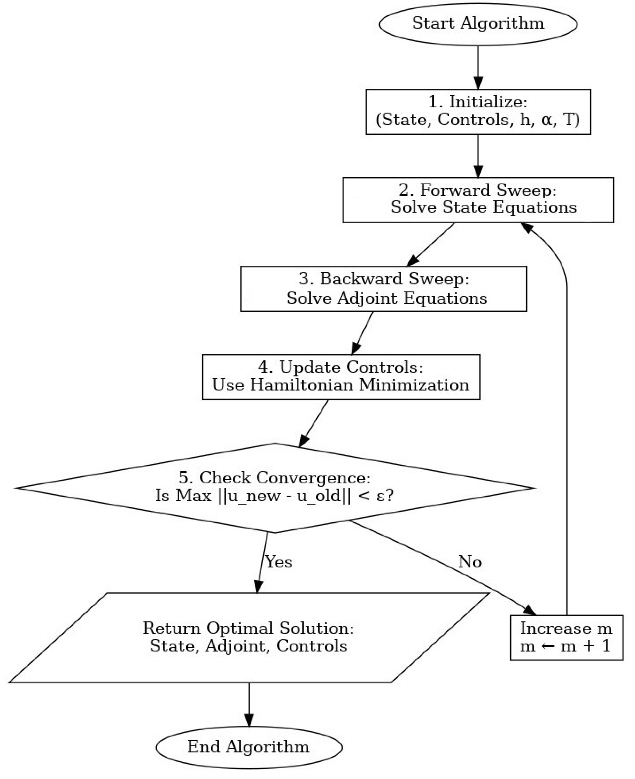
The system (97) is solved recursively using Newton’s method due to its nonlinear dependence on . To solve the optimal control problem, we apply the forward-backward sweep algorithm. First, the state equations in (80) are integrated forward in time using the above numerical method and initial conditions. Then, the adjoint equations in (88)—derived from the Hamiltonian—are solved backward in time using the transversality conditions. At each iteration, the control variables to are updated by minimizing the Hamiltonian function, according to the characterizations provided by the necessary optimality conditions in (91). The overall procedure is summarized below:
| Algorithm 1 (Forward–backward sweep method for solving the fractional optimal control problem) |
|
Figure 2.
Flowchart of the forward–backward sweep algorithm.
5.1. Convergence Analysis
The primary goal of the convergence analysis in our study is to demonstrate that the numerical method used to approximate the solution of the fractional-order optimal control system converges to the true solution as the step size . Recall the integral approximation error in the fractional trapezoidal method, given by:
where is the numerical approximation of the state vector at node . Subtracting the exact integral representation from its numerical approximation yields the error:
where , are trapezoidal weights, and is the local truncation error of the quadrature rule. Assuming that satisfies a Lipschitz condition with constant L, and letting , , we have:
For sufficiently small h, the following recursive bound applies:
which leads to:
Therefore, as , we conclude that , proving the convergence of the numerical scheme for the fractional-order epidemic model with optimal control.
6. Numerical Results
In the numerical simulations, we applied the method described in Section 5, implemented using the Python software. Furthermore, we consider various simulation scenarios, which we will discuss hereinafter.
6.1. Simulation Scenarios
To assess the effectiveness of various intervention strategies in mitigating the spread of ACL, we define a set of control-based simulation scenarios. Each scenario corresponds to a distinct combination of the four available control functions in our model: use of bed nets and repellents (), treatment of symptomatic individuals (), insecticide spraying (), and awareness campaigns (). These controls are applied subject to resource constraints, and their configurations are chosen to reflect both practical public health policies and theoretical significance. The following scenarios are considered:
-
Scenario S1 (Vector Avoidance Only): Figure 3 illustrates the temporal evolution of all ten state variables under Scenario , where only the personal protection control (e.g., use of bed nets and repellents) is active, and compares it to the uncontrolled baseline. The fractional order is fixed at to account for memory effects inherent in both the biological and behavioral dynamics of the system. The implementation of significantly reduces the force of infection between humans and vectors by lowering effective contact rates. As a result, a modest yet consistent decline is observed in the number of exposed () and symptomatic infected humans () throughout the simulation period, relative to the no-control scenario. The impact on asymptomatic infections () is less pronounced, given their indirect dependence on exposure rather than contact intensity. For the vector population, a slight reduction in exposed () and infected vectors (, ) is observed due to the reduced likelihood of acquiring infection from protected human hosts. However, since vector dynamics are not directly targeted in this scenario, the changes are relatively subdued. Importantly, the awareness function shows no deviation between the two cases, as no awareness-related control is employed.Overall, Scenario demonstrates that personal protection can contribute meaningfully to reducing human infections, especially during the early and middle phases of the outbreak. However, its isolated application yields limited control over the broader transmission cycle, suggesting that more comprehensive strategies are required to achieve substantial disease suppression.
-
Scenario S2 (Treatment Only): Figure 4 presents the model dynamics under Scenario , where treatment of symptomatic individuals via control is the sole intervention. Compared to the baseline, a marked reduction in the symptomatic infected population () is achieved, particularly evident during the early and mid stages of the epidemic. This decline results from a shortened infectious period, which also indirectly reduces secondary infections.Consequently, a delayed but observable decline in the number of exposed humans () emerges due to the weakened forward transmission. The asymptomatic class (), unaffected directly by treatment, exhibits minor differences from the baseline. For the vector populations, a mild reduction in exposed and infected compartments (, , ) occurs, driven by the lowered human-to-vector transmission intensity. No change is observed in the awareness level (), as no awareness-related intervention is employed. Overall, Scenario proves effective in rapidly reducing symptomatic infections and partially suppressing the transmission cycle, but it does not fully disrupt vector-driven dynamics without complementary controls
-
Scenario S3 (Vector Spraying Only): Figure 5 depicts the evolution of state variables under Scenario , where insecticide spraying () is the only active control. The most pronounced impact is observed in the vector-related compartments, with substantial reductions in susceptible (), exposed (), and both infected classes (, ), indicating the direct mortality effect of the intervention on the vector population. This reduction in vector density effectively lowers the force of infection toward humans, leading to a delayed but meaningful decline in exposed () and symptomatic infected humans (). The asymptomatic class (), being indirectly affected, also exhibits a slight downward shift compared to the no-control case.Since treatment and awareness controls are inactive, the recovery and awareness levels (, ) follow trajectories similar to the baseline. Overall, vector spraying in isolation demonstrates notable efficiency in disrupting vector dynamics and indirectly suppressing human transmission, though it falls short of completely halting disease propagation in the absence of host-directed interventions.
-
Scenario S4 (Awareness Campaign Only): Figure 6 shows the system trajectories under Scenario , where only public awareness efforts () are implemented. As expected, the awareness level exhibits a sustained and significant increase over time, reflecting the direct effect of the control. This rise in awareness reduces the effective contact rate between humans and vectors, which in turn mildly suppresses transmission. The impact on epidemiological compartments is modest but consistent: small reductions are observed in the exposed (), symptomatic (), and asymptomatic () human classes, along with slight decreases in infected vectors (, ). However, due to the indirect nature of this intervention and the absence of direct treatment or vector-killing measures, the declines are not pronounced.Overall, Scenario highlights the role of behavioral modification as a supportive control. While awareness alone does not significantly alter the disease trajectory, it contributes to reducing transmission intensity, especially when integrated with other strategies.
-
Scenario S5 (Combined Treatment and Personal Protection): Figure 7 illustrates the dynamics under Scenario , which combines personal protection () and treatment of symptomatic individuals (). This dual intervention targets both the infection source and the transmission pathway, leading to a more pronounced suppression of the epidemic compared to single-control strategies. A significant reduction in symptomatic infections () is observed, resulting from both shortened infectious periods and decreased exposure risk. The exposed class () also declines notably, benefiting from the synergistic effect of reduced contact and diminished secondary transmission. Asymptomatic infections (), while not directly treated, follow a downward trend as a result of reduced upstream exposure. In the vector population, moderate declines are observed in exposed and infected compartments due to the reduced infectivity of human hosts. Since no vector-targeted control or awareness campaign is applied, the susceptible vector pool () and awareness level () remain largely unchanged.Overall, Scenario demonstrates the enhanced effectiveness of integrated host-based strategies. The simultaneous use of repellents and treatment significantly weakens transmission feedback loops and offers a balanced approach to disease mitigation
-
Scenario S6 (Combined Repellent and Spraying): Figure 8 presents the evolution of the system under Scenario , which integrates personal protection () with insecticide spraying (). This combined strategy simultaneously reduces human-vector contact and vector abundance, resulting in a strong and rapid suppression of disease transmission. The vector-related compartments (, , , ) show substantial declines due to direct vector mortality induced by spraying. Additionally, the reduction in human exposure—achieved through repellents and bed nets—further limits the replenishment of the infected vector pool. On the human side, exposed (), symptomatic (), and asymptomatic () infections are all significantly reduced relative to the baseline. These improvements stem from the combined impact of fewer infectious bites and diminished forward transmission pressure. However, since no treatment or awareness interventions are applied, recovery dynamics and the awareness level remain nearly identical to the uncontrolled case.In summary, Scenario effectively disrupts both the environmental and behavioral transmission routes. It proves particularly valuable in settings where vector control and personal-level measures can be deployed in tandem, even in the absence of clinical or educational interventions.
-
Scenario S7 (Combined Treatment and Awareness): Figure 9 depicts the model behavior under Scenario , which combines treatment of symptomatic individuals () with public awareness campaigns (). This hybrid approach merges direct clinical intervention with indirect behavioral modification, resulting in meaningful reductions across several compartments. Symptomatic infections () decline sharply due to active treatment, which shortens the infectious period and interrupts human-to-vector transmission. At the same time, the awareness function increases steadily, decreasing exposure risk by reducing contact rates. These complementary effects yield a visible drop in the number of exposed humans (), as well as a moderate decline in asymptomatic infections (), which are indirectly influenced by reduced incidence. Although the vector compartments are not targeted directly, a slight reduction in infected vectors (, ) emerges due to decreased transmission from human hosts. As expected, the susceptible vector population () remains stable in the absence of vector-specific controls.Scenario illustrates the added value of combining behavioral and therapeutic strategies. The synergy between heightened public awareness and timely clinical response provides a two-pronged mechanism for curbing transmission, especially in human-dominated settings.
-
Scenario S8 (Full Control Strategy): Figure 10 shows the dynamics of the full intervention scenario , in which all four controls—personal protection (), treatment (), insecticide spraying (), and public awareness ()—are simultaneously applied. This comprehensive strategy exerts maximal pressure on the disease system by targeting both human and vector dynamics as well as behavioral responses. The result is a pronounced and rapid decline in all key epidemiological compartments. Symptomatic () and asymptomatic () infections are significantly reduced due to the combined effects of reduced exposure, enhanced recovery, and increased awareness. The exposed human class () also decreases sharply, reflecting strong suppression of transmission at early stages. Vector-related states—including , , , and —drop substantially as a consequence of direct vector mortality (via ) and indirect transmission reductions. Moreover, the awareness level rises steadily, further reinforcing the behavioral shift needed to sustain control measures.Overall, Scenario delivers the most effective outcome among all considered strategies. By synchronizing environmental, clinical, and educational interventions, it disrupts multiple feedback loops in the transmission cycle and highlights the power of integrated public health approaches in managing ACL.
6.2. Effect of Fractional Order
Figure 11 demonstrates the influence of the fractional derivative order on the temporal evolution of symptomatic infections and the awareness level under Scenario , where only the awareness control is active. As the value of decreases from 1.0 to 0.7, representing a stronger memory effect, a significant suppression in both the peak and the long-term prevalence of is observed. This behavior reflects the capacity of fractional-order dynamics to capture the prolonged impact of public health campaigns, where awareness persists and continues to influence behavior over time. Furthermore, the awareness variable exhibits a faster and more sustained increase at lower , implying that individuals respond more effectively to information and retain it longer when memory effects are stronger. Overall, the results highlight that fractional models can provide a more realistic representation of behavioral and epidemiological processes, and that awareness campaigns may become considerably more effective in the presence of population memory and behavioral inertia. Figure 12 illustrates the effect of the fractional-order parameter on the dynamics of symptomatic infections and awareness level under Scenario , where all four control strategies ( to ) are simultaneously active. The figure shows that as decreases from 1.0 to 0.7, both the peak and the duration of symptomatic infections are further reduced, with the earliest suppression occurring at . This enhanced mitigation highlights the memory effect embedded in the fractional derivative: a lower means that the system retains more information from the past, thereby making the control interventions—particularly awareness and behavioral changes—more effective over time. Similarly, the awareness function increases more rapidly and reaches higher sustained levels at lower , reinforcing the idea that memory-dependent behavioral responses can amplify the impact of multi-faceted control programs. Overall, these findings emphasize that the synergy between fractional memory and combined interventions can significantly accelerate disease eradication.
Figure 13 shows how the objective functional varies with the fractional-order derivative across different intervention scenarios. As increases toward the classical case , the values of generally increase for all scenarios. This trend reflects the reduced impact of memory effects in integer-order models, where the system responds more locally in time and lacks long-term behavioral persistence. In contrast, lower values of (e.g., ) lead to significantly lower values of , indicating enhanced cost-effectiveness of control strategies under fractional dynamics. The memory effect embedded in the Caputo derivative allows past control efforts—especially in awareness and behavioral response—to exert influence over extended periods, thus reducing both infection burden and intervention costs more efficiently. Notably, scenarios with multiple active controls (e.g., Scenario S8) exhibit the greatest sensitivity to , suggesting that fractional-order models are particularly valuable in optimizing complex, multi-layered intervention programs.
6.3. Optimal Scenario Identification
To determine the most effective intervention strategy, we compare the total cost functional J and accumulated infection burden E across all control scenarios for the fractional-order , as shown in Table 5. The scenario involving no control results in the highest infection burden with a baseline cost of . The lowest value of J is achieved by the scenario with , which also substantially reduces the infection burden to . Interestingly, adding awareness control to this combination ( or “All Controls”) does not significantly improve either cost or effectiveness, suggesting a redundancy or saturation effect when all interventions are simultaneously applied. Scenarios that employ only awareness (), or only bed-net usage (), result in nearly identical infection levels to the no-control case, but with a higher total cost. This indicates that awareness campaigns alone—although valuable from a public health perspective—are insufficient to control the disease without complementary biomedical interventions such as treatment or vector control. These findings are quantitatively confirmed by the Incremental Cost-Effectiveness Ratio (ICER) values in Table 6. The scenario exhibits the lowest ICER of , indicating a cost-saving effect relative to no control. In contrast, scenarios with only or yield highly inefficient outcomes, with ICER values exceeding 1900 and 36000 respectively. Even the “All Controls” scenario, despite achieving a slightly reduced infection level, shows a less favorable ICER compared to due to higher costs. In summary, the optimal control configuration in terms of cost-effectiveness and infection mitigation is the combined treatment and spraying scenario . This highlights the biological importance of directly targeting disease progression and vector transmission rather than relying solely on awareness or preventive measures.
6.4. Scientific Interpretation, Policy and Public Health Implications, and Comparison with Classical Control Models
The present study proposes a novel fractional optimal control model for ACL, integrating key epidemiological features such as asymptomatic transmission, vector resistance, and behaviorally-driven awareness dynamics. By employing Caputo fractional derivatives, the model captures non-local temporal effects inherent to biological and behavioral processes, such as memory of past exposures or sustained public responses to interventions [10,23].
Scientifically, one of the major innovations is the explicit modeling of the asymptomatic human class, which reflects sub-clinical carriers who sustain transmission without detection or treatment. Previous studies have shown that ignoring asymptomatic individuals can result in underestimation of disease burden and intervention failure [19,20]. Our simulations confirm that targeting only symptomatic individuals leads to limited impact unless asymptomatic transmission is also suppressed. Another key contribution is the inclusion of a resistant vector compartment, modeling the gradual emergence of insecticide resistance—a growing concern in leishmaniasis-endemic regions [4]. The model demonstrates that even a small fraction of resistant vectors can significantly erode the effectiveness of vector control measures over time, supporting the call for resistance monitoring and rotation of control tools as recommended by WHO [32].
The introduction of a dynamic awareness function allows for the simulation of behaviorally adaptive responses in the human population. This component, which evolves based on campaign effort and decays in the absence of reinforcement, aligns with current findings in behavioral epidemiology that emphasize the time-dependent and nonlinear nature of public health compliance [14]. Under fractional-order dynamics, awareness campaigns exhibit greater long-term persistence and efficacy due to memory effects, highlighting the relevance of fractional modeling for socio-epidemiological systems [11]. From a policy and public health perspective, the model provides an actionable framework for resource-aware control planning. Through optimal control theory, it identifies dynamic strategies for allocating limited resources across treatment, protection, spraying, and education. Numerical results show that combinations such as treatment + vector spraying outperform single strategies in terms of cost-effectiveness—quantified via the objective functional and ICER values—especially under high transmission scenarios. These results are consistent with prior work on cost-effective leishmaniasis control in resource-constrained settings [24].
When compared to classical integer-order control models, the proposed fractional model offers notable advantages. Classical models assume memory-less dynamics and typically fail to capture delayed or accumulated effects of interventions. As demonstrated in previous research [21,22], fractional-order systems can reflect biologically realistic features such as incubation delays, treatment response variability, and behavioral inertia. Moreover, the smoother control profiles generated by the fractional approach (as opposed to abrupt switching seen in classical settings) are more compatible with real-world health program logistics and behavioral adaptation lags. In summary, this study extends the theoretical framework of disease modeling by incorporating biologically meaningful memory mechanisms, resistance evolution, and awareness-driven behavior into a single, resource-constrained fractional optimal control model. It bridges the gap between rigorous mathematical modeling and applied public health policy, and offers valuable insight into designing robust and sustainable intervention strategies for ACL and similar vector-borne diseases.
7. Conclusion and Future Work
This study presents a novel fractional-order optimal control model for ACL, capturing the complexities of disease dynamics through the integration of asymptomatic carriers, insecticide-resistant vectors, and behaviorally adaptive awareness. The use of Caputo fractional derivatives enables the model to reflect memory-dependent processes in both biological and behavioral domains, such as incubation delays, persistent public health responses, and the long-term evolution of resistance.
Key findings from the analysis highlight the importance of incorporating memory effects into epidemiological models. Our results show that intervention strategies such as treatment and vector spraying are significantly more effective under fractional-order dynamics (), as they benefit from the sustained effects of past actions. Additionally, modeling public awareness as a dynamic state variable — rather than a static parameter — allows the model to reflect intervention fatigue and the temporal evolution of behavior change. This is in line with recent behavioral modeling frameworks which emphasize feedback mechanisms in public response [15,16].
The model also illustrates that the presence of asymptomatic individuals can perpetuate transmission even in the presence of symptomatic treatment programs, underscoring the need for broader surveillance approaches [1]. Moreover, simulations involving insecticide-resistant vectors suggest that traditional spraying interventions may lose efficacy over time unless resistance management strategies are implemented. The biological relevance of these extensions demonstrates the model’s ability to bridge mathematical rigor with epidemiological realism.
From a public health perspective, the optimal control framework provides practical insights into how limited resources can be allocated among multiple interventions. In particular, combinations of interventions — especially treatment and vector control — are shown to yield high cost-effectiveness, while awareness-only strategies, although slower, produce more sustainable effects under memory-rich dynamics. These findings complement recent theoretical and empirical research emphasizing the role of long-term planning in epidemic control [12].Despite its strengths, the model has limitations. It assumes homogeneous population mixing and does not incorporate spatial heterogeneity or network-based interactions, which have been shown to significantly affect disease spread and control outcomes [33]. Additionally, some parameters — particularly those related to behavioral response and resistance evolution — were estimated or assumed in the absence of high-quality empirical data.
Future research may address these limitations through several directions. First, integrating stochastic effects and uncertainty analysis would enhance model robustness, especially under real-world unpredictability [34]. Second, applying Bayesian inference or machine learning methods to estimate behavioral and biological parameters from field data would improve the model’s predictive accuracy [13]. Third, incorporating spatial structure and meta-population dynamics — including human mobility and network connectivity — could reveal more nuanced transmission patterns and inform targeted intervention strategies [35]. Finally, expanding the model to account for co-infections (e.g., HIV-Leishmania) or immune memory effects may increase its relevance for broader public health contexts [36]. In summary, this work introduces a biologically meaningful and mathematically robust framework for modeling ACL, offering both theoretical innovation and practical policy implications. The use of fractional calculus enriches our understanding of memory-driven dynamics in disease transmission and control, making this approach valuable not only for ACL but also for a wide range of persistent vector-borne diseases.
Author Contributions
Conceptualization, A.E.; software, A.E.; validation, A.J.; formal analysis, M.Y.; investigation, M.Y.; visualization, M.Y.; writing—original draft, A.E.; writing—review and editing, A.J.; supervision, A.J. All authors have read and agreed to the published version of the manuscript.
Funding
This research received no external funding.
Data Availability Statement
No data was used for the research described in the article.
Conflicts of Interest
The authors declare no conflict of interest.
References
- Alvar, J. , Vélez, I. D., Bern, C., Herrero, M., Desjeux, P., Cano, J.,... & the WHO Leishmaniasis Control Team, Leishmaniasis worldwide and global estimates of its incidence, PLoS One, 7(5) (2012) e35671.
- Cosma, C. , Maia, C., Khan, N., Infantino, M., & Del Riccio, M., Leishmaniasis in humans and animals: A one health approach for surveillance, prevention and control in a changing world, Tropical Medicine and Infectious Disease, 9(11) (2024) 258.
- Almeida-Souza, F. , Calabrese, K. D. S., Abreu-Silva, A. L., &; Cardoso, F., Leishmania Parasites: Epidemiology, Immunopathology and Hosts, BoD–Books on Demand, 2024. [Google Scholar]
- Khater, H. F. , & Ramadan, M. Y., Control of phlebotomine sandflies (Diptera: Psychodidae) with insecticides: A review of current status and future prospects, Journal of Vector Ecology, 38(1) (2013) 1–9.
- Hethcote, H. W. , The mathematics of infectious diseases, SIAM Review, 42(4) (2000) 599-653.
- Van den Driessche, P. , & Watmough, J., Reproduction numbers and sub-threshold endemic equilibria for compartmental models of disease transmission, Mathematical Biosciences, 180(1–2) (2002) 29-48. [CrossRef]
- Safan, M. , & Altheyabi, A., Mathematical analysis of an anthroponotic cutaneous leishmaniasis model with asymptomatic infection, Mathematics, 11(10) (2023) 2388. [CrossRef]
- Sinan, M. , Ansari, K. J., Kanwal, A., Shah, K., Abdeljawad, T., & Abdalla, B., Analysis of the mathematical model of cutaneous leishmaniasis disease, Alexandria Engineering Journal, 72 (2023) 117-134. [CrossRef]
- Biswas, D. , Dolai, S., Chowdhury, J., Roy, P. K., & Grigorieva, E. V., Cost-effective analysis of control strategies to reduce the prevalence of cutaneous leishmaniasis, based on a mathematical model, Mathematical and Computational Applications, 23(3) (2018) 38. [CrossRef]
- Diethelm, K. , The Analysis of Fractional Differential Equations: An Application-Oriented Exposition Using Differential Operators of Caputo Type, Springer, 2010.
- Baleanu, D. , Losada, J., & Jarad, F., Nonlocal modeling and analysis of the memory-dependent SIR epidemic system, Applied Mathematical Modelling, 65 (2019) 123-137.
- Li, Q. , Peng, Y., & Bai, X., Memory-dependent fractional-order model of COVID-19 with public psychological effects, Applied Mathematical Modelling, 90 (2021) 1062–1080.
- Yoon, J. , Saha, S., & Kalantari, A., Bayesian parameter estimation for fractional-order epidemiological models: A case study of COVID-19, Mathematics, 10(5) (2022) 822.
- Funk, S. , Gilad, E., & Jansen, V. A. A., The spread of awareness and its impact on epidemic outbreaks, Proceedings of the National Academy of Sciences, 106(16) (2009) 6872-6877. [CrossRef]
- Verelst, F. , Willem, L., &; Beutels, P., Behavioural change models for infectious disease transmission: A systematic review (2010–2015), Journal of the Royal Society Interface, 13(125) (2016) 20160820. [Google Scholar]
- Van Bavel, J. J. , Baicker, K., Boggio, P. S., Capraro, V., Cichocka, A., Cikara, M.,... & Willer, R., Using social and behavioural science to support COVID-19 pandemic response, Nature Human Behaviour, 4(5) (2020) 460-471. [CrossRef]
- Lenhart, S. , & Workman, J. T., Optimal Control Applied to Biological Models, Chapman & Hall/CRC, 2007.
- Pantha, B. , Agusto, F. B., & Elmojtaba, I. M., Optimal Control Applied to a Visceral Leishmaniasis Model, Technical Report, Department of Mathematics, Texas State University, 2020. [CrossRef]
- Nadeem, F. , Zamir, M., & Tridane, A., Modeling and control of zoonotic cutaneous leishmaniasis, Punjab University Journal of Mathematics, 51(2) (2019) 105-121.
- Zamir, M. , Zaman, G., & Alshomrani, A. S., Sensitivity analysis and optimal control of anthroponotic cutaneous leishmania, PLoS One, 11(8) (2016) e0160513.
- Kilbas, A. A. , Srivastava, H. M., & Trujillo, J. J., Theory and Applications of Fractional Differential Equations, Elsevier, 2006.
- Machado, J. A. T. , Kiryakova, V., & Mainardi, F., Recent history of fractional calculus, Communications in Nonlinear Science and Numerical Simulation, 16(3) (2011) 1140–1153. [CrossRef]
- Mainardi, F. , Fractional Calculus and Waves in Linear Viscoelasticity: An Introduction to Mathematical Models, Imperial College Press, 2010.
- Toufga, H. , Sakkoum, A., Benahmadi, L., & Lhous, M., Analysis of the dynamics and optimal control of cutaneous Leishmania during human immigration, Iranian Journal of Numerical Analysis and Optimization, 15(1) (2025) 311-345.
- Khan, A. , Zarin, R., Inc, M., Zaman, G., & Almohsen, B., Stability analysis of Leishmania epidemic model with harmonic mean type incidence rate, European Physical Journal Plus, 135(6) (2020) 528. [CrossRef]
- Podlubny, I. , Fractional Differential Equations: An Introduction to Fractional Derivatives, Fractional Differential Equations, to Methods of Their Solution and Some of Their Applications, Academic Press, 1999.
- Marino, S. , Hogue, I. B., Ray, C. J., & Kirschner, D. E., A methodology for performing global uncertainty and sensitivity analysis in systems biology, Journal of Theoretical Biology, 254(1) (2008) 178-196. [CrossRef]
- Belser, A. B. , McKay, C. L., McMahon, D. K., & Hittner, J. B., Global sensitivity analysis: Concepts, methods, and applications in public health modeling, BMC Public Health, 22 (2022) 1-14.
- Wu, J. , Dhingra, R., Gambhir, M., &; Remais, J. V., Sensitivity analysis of infectious disease models: Methods, advances and their application, Journal of the Royal Society Interface, 10(86) (2013) 20121018. [Google Scholar]
- Saltelli, A. , Ratto, M., Andres, T., Campolongo, F., Cariboni, J., Gatelli, D.,... &; Tarantola, S., Global Sensitivity Analysis: The Primer, John Wiley & Sons, 2008. [Google Scholar]
- Sobie, E. A. , Parameter sensitivity analysis in electrophysiological models using multivariable regression, Biophysical Journal, 96(4) (2009) 1264-1274. [CrossRef]
- World Health Organization, Vector control in leishmaniasis: Current strategies and future directions, WHO Technical Report, 2020.
- Kiss, I. Z. , Miller, J. C., &; Simon, P. L., Mathematics of Epidemics on Networks: From Exact to Approximate Models, Springer, 2017. [Google Scholar]
- Allen, L. J. S. , A primer on stochastic epidemic models: Formulation, numerical simulation, and analysis, Infectious Disease Modeling, 2(2) (2017) 128-142. [CrossRef]
- Pastor-Satorras, R. , Castellano, C., Van Mieghem, P., & Vespignani, A., Epidemic processes in complex networks, Reviews of Modern Physics, 87(3) (2015) 925–979.
- Ferrer, R. A. , &; Klein, W. M., Examining the impact of co-infection in neglected tropical diseases: A theoretical modeling approach, PLoS Neglected Tropical Diseases, 15(4) (2021) e0009333. [Google Scholar]
Figure 1.
Global sensitivity analysis (PRCC).
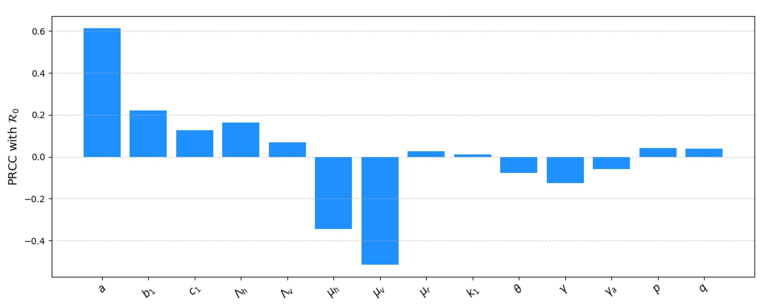
Figure 3.
Comparison of state variables under Scenario and the uncontrolled baseline.
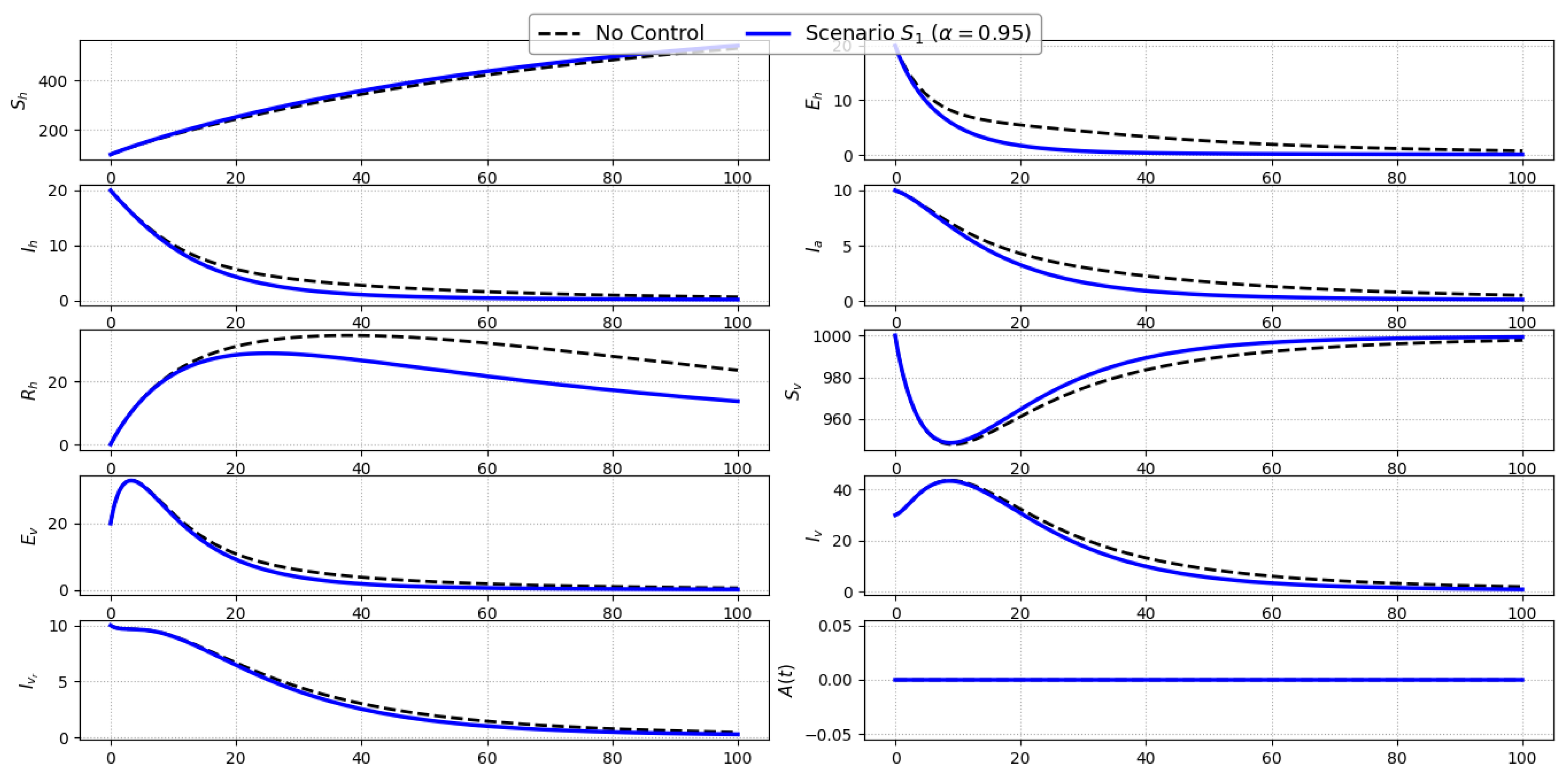
Figure 4.
Comparison of state variables under Scenario and the uncontrolled baseline.
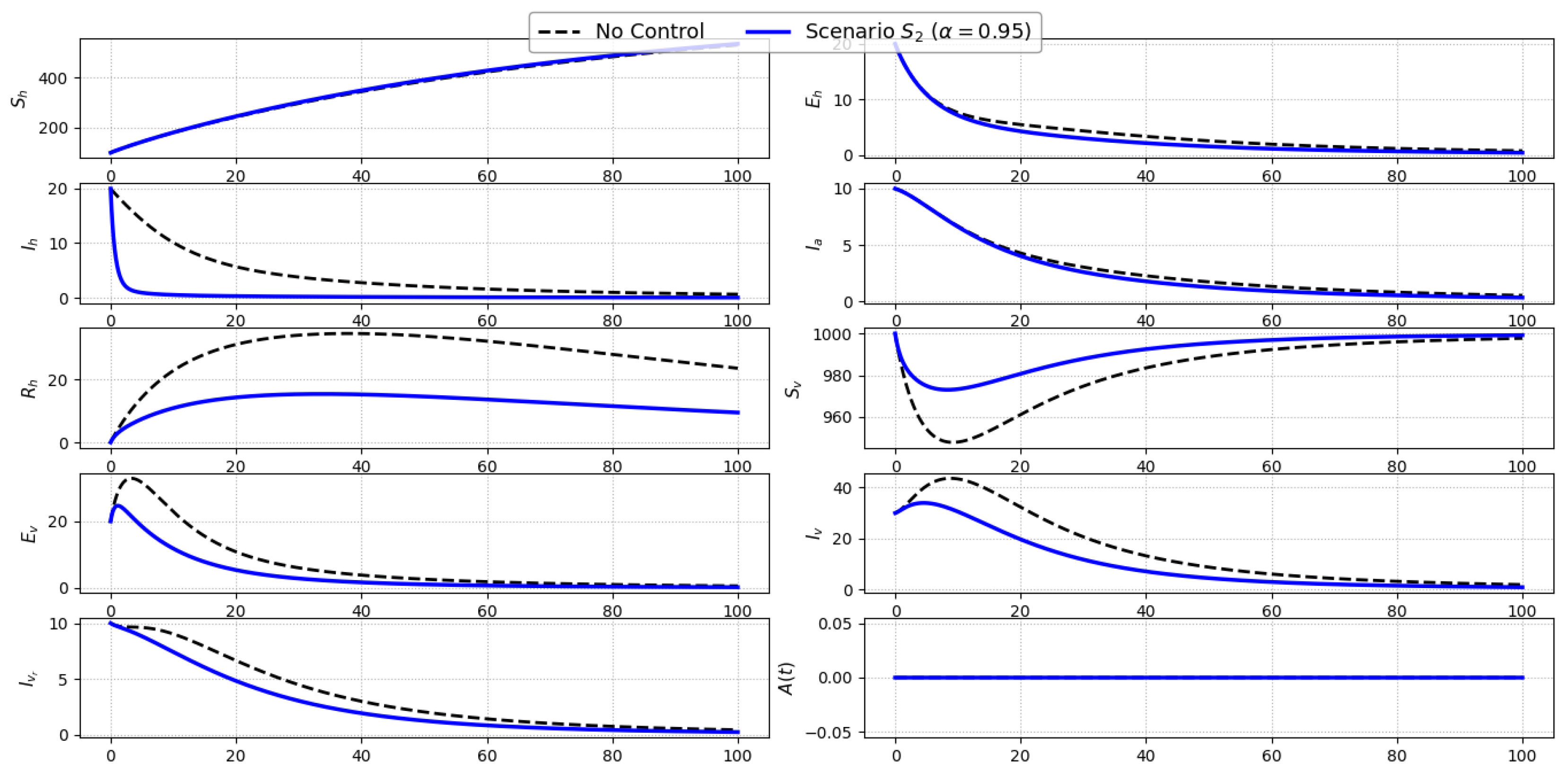
Figure 5.
Comparison of state variables under Scenario and the uncontrolled baseline.
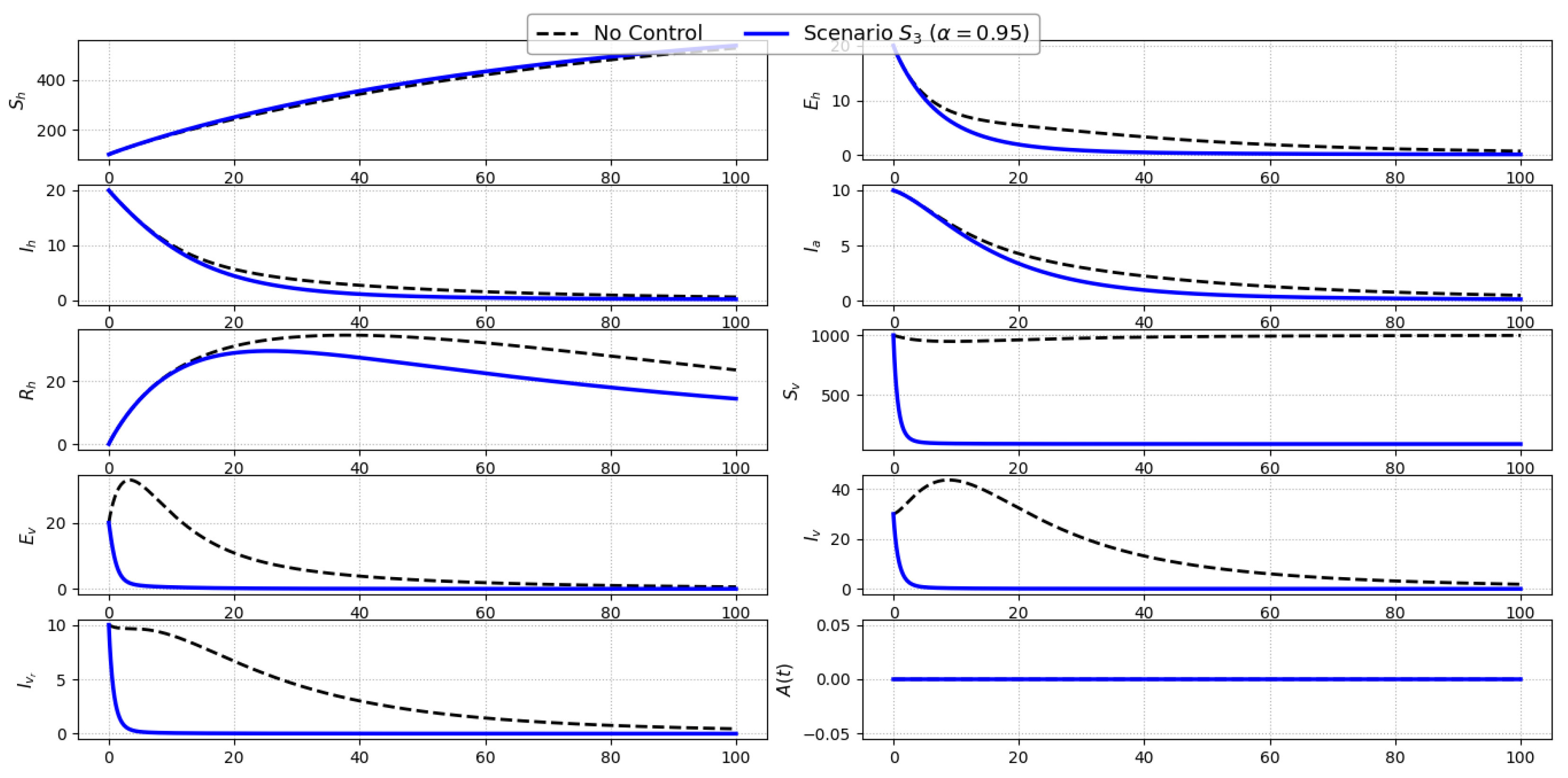
Figure 6.
Comparison of state variables under Scenario and the uncontrolled baseline.
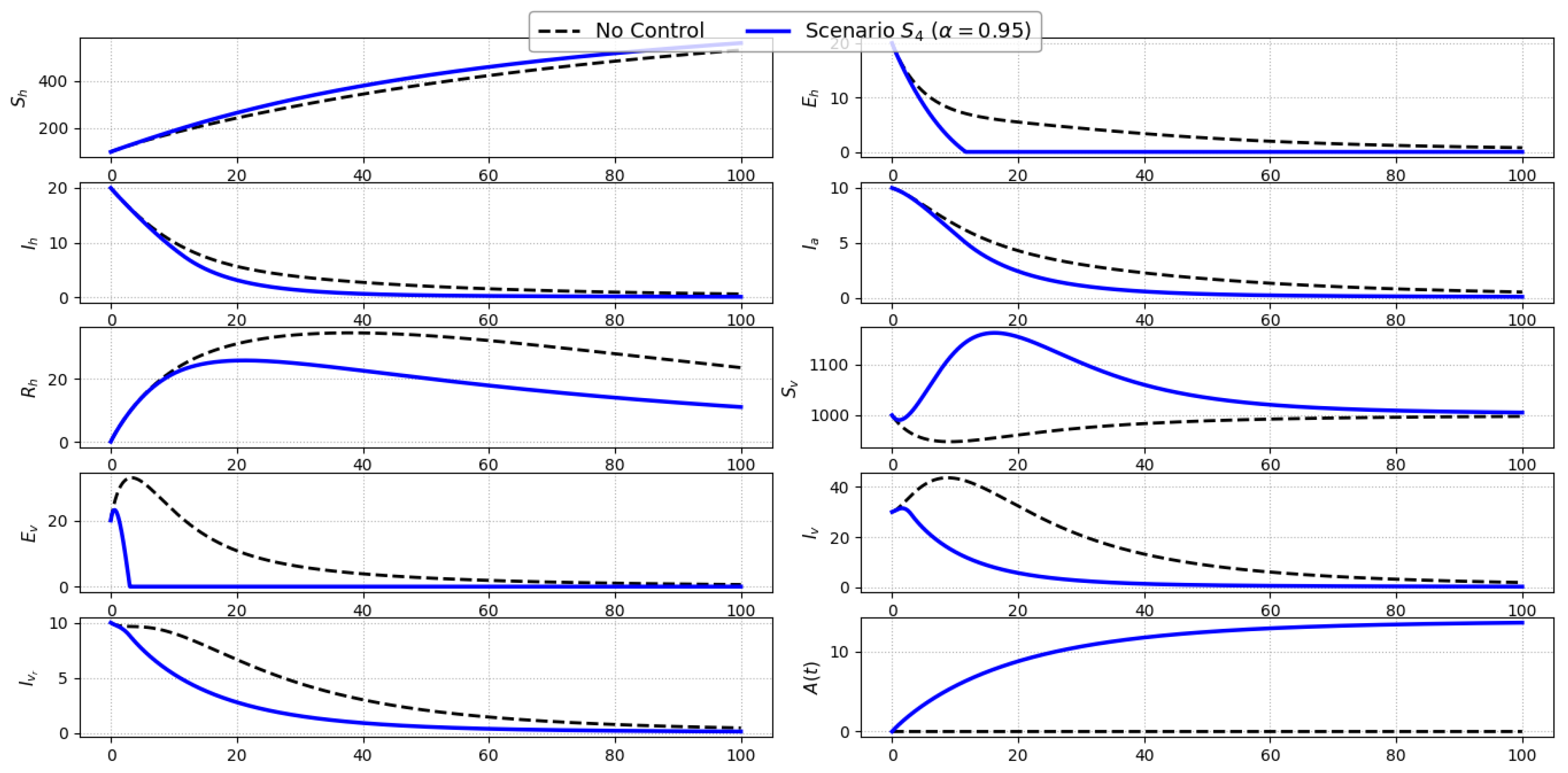
Figure 7.
Comparison of state variables under Scenario and the uncontrolled baseline.
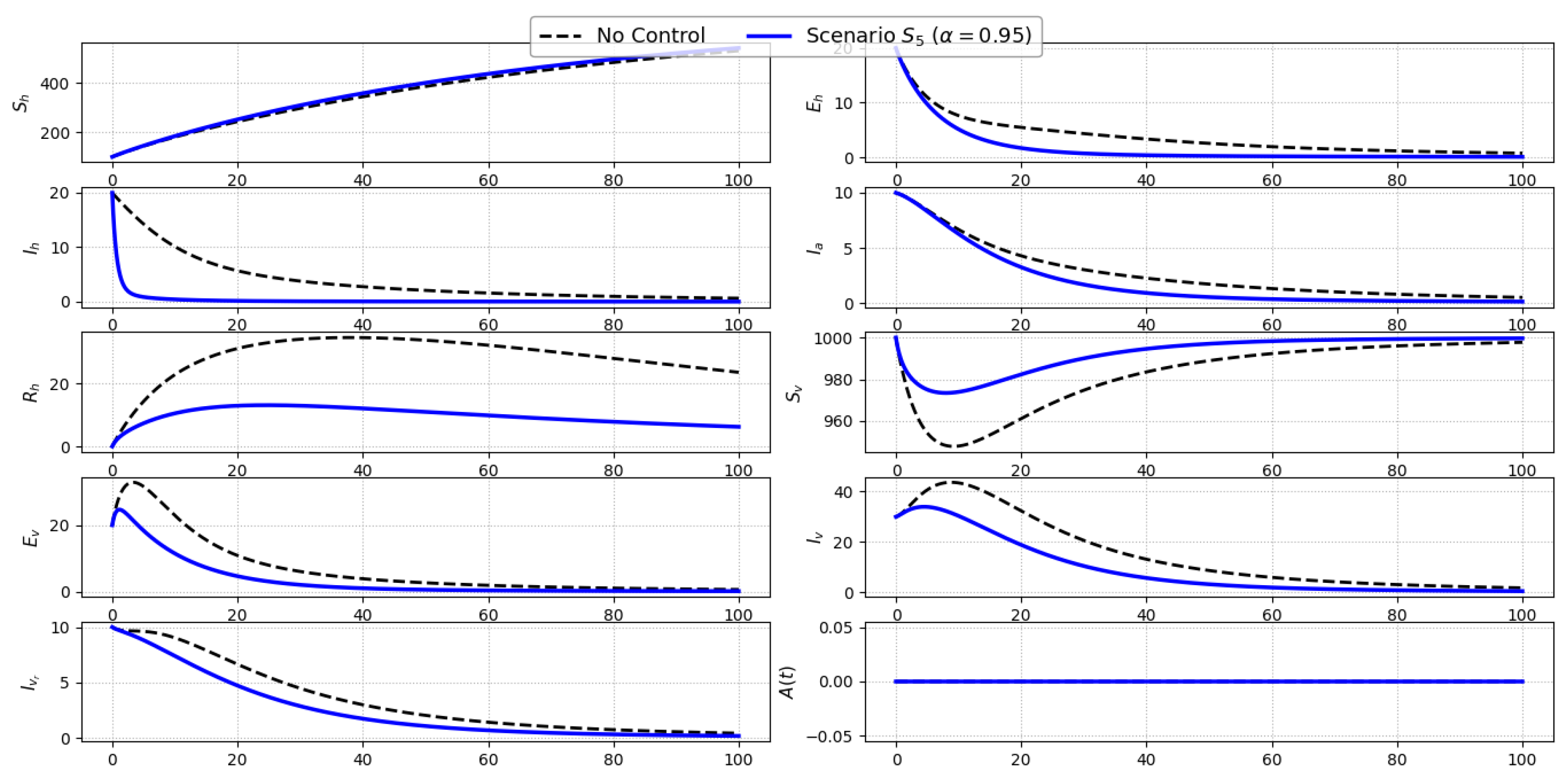
Figure 8.
Comparison of state variables under Scenario and the uncontrolled baseline.

Figure 9.
Comparison of state variables under Scenario and the uncontrolled baseline.
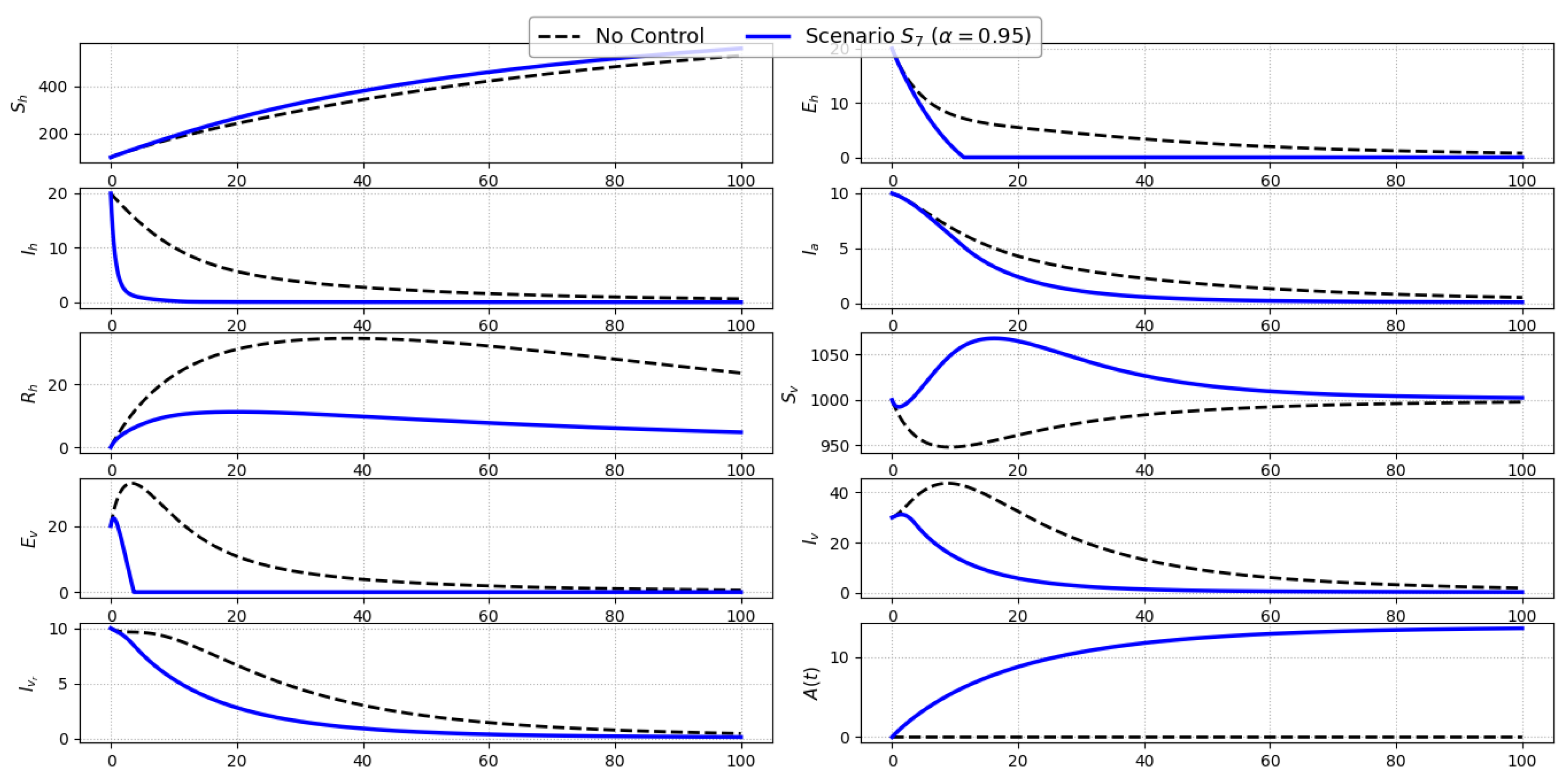
Figure 10.
Comparison of state variables under Scenario and the uncontrolled baseline.
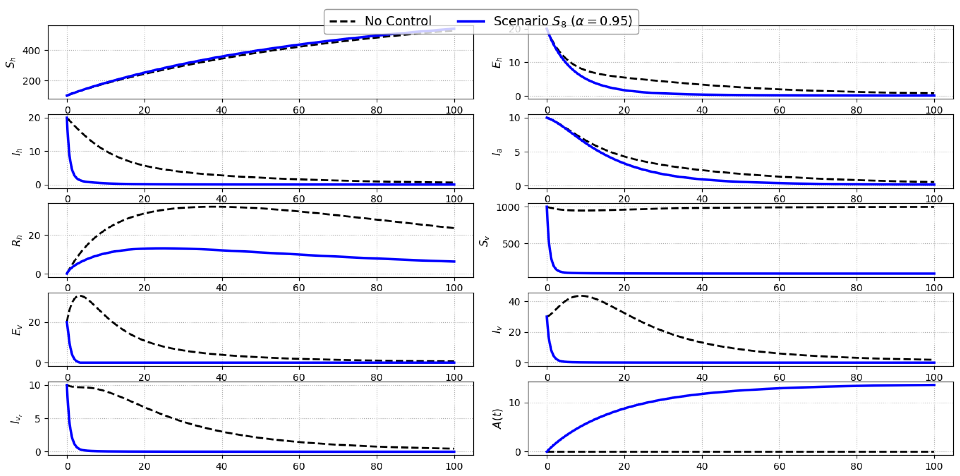
Figure 11.
Effect of parameter under scenario .
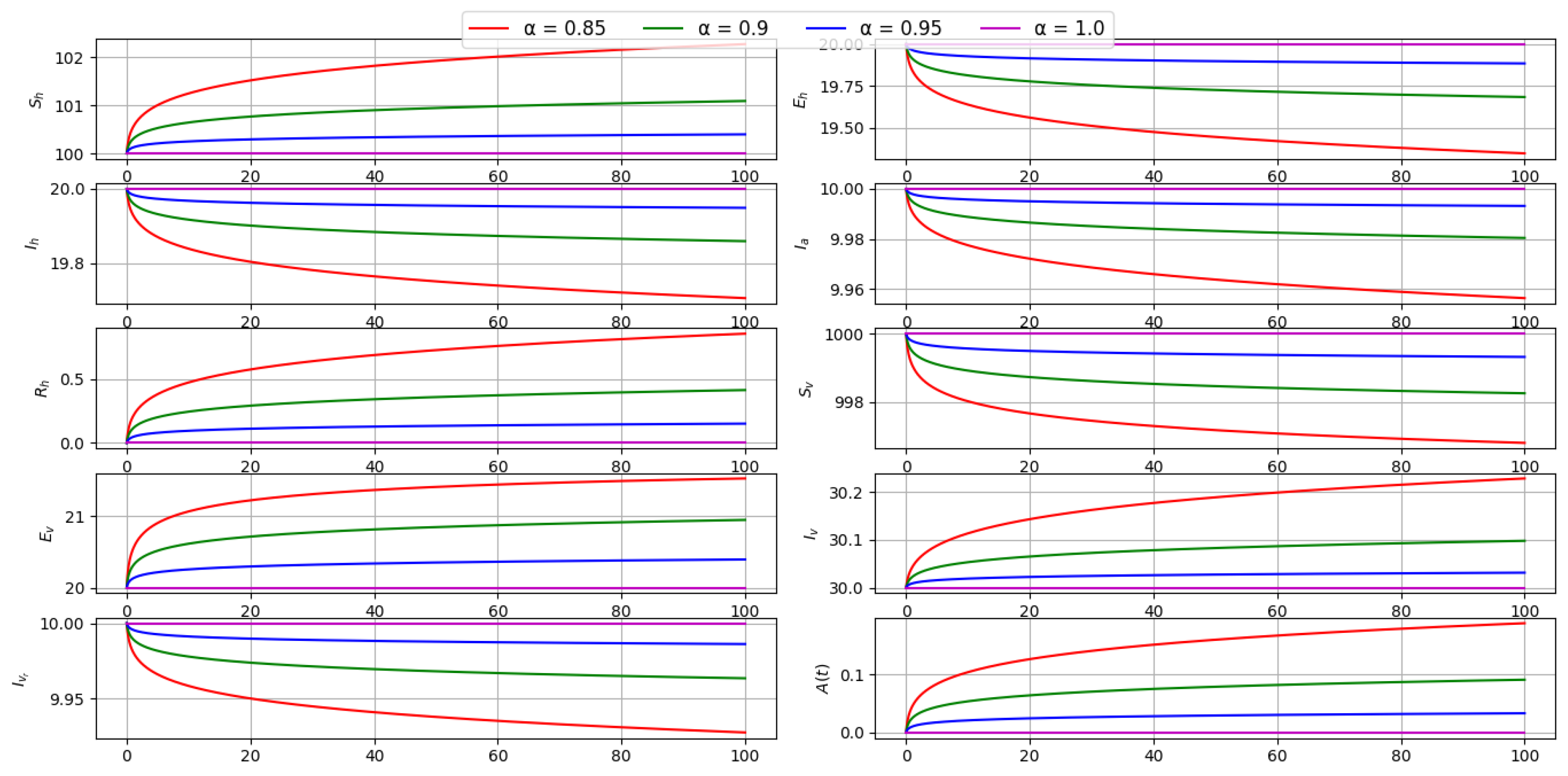
Figure 12.
Effect of parameter under scenario .
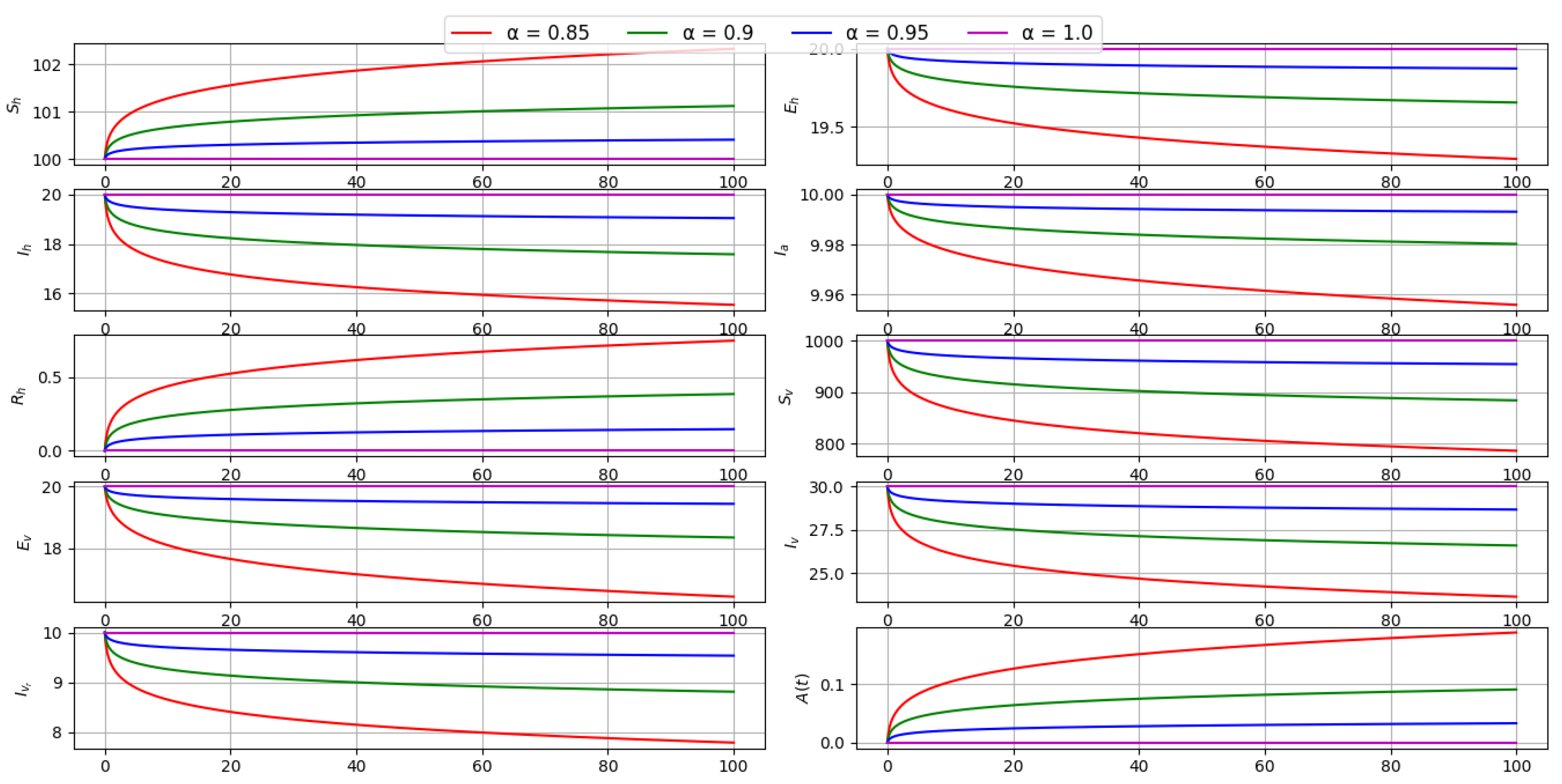
Figure 13.
Effect of the fractional derivative order on the objective functional across different control scenarios.
Figure 13.
Effect of the fractional derivative order on the objective functional across different control scenarios.
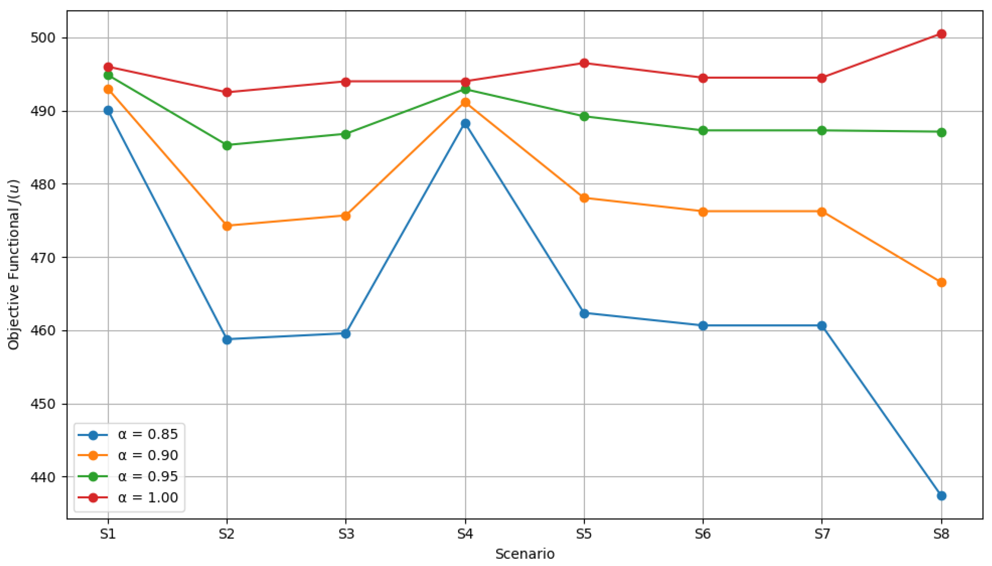

Table 1.
State variables and their initial conditions at .
| Variable | Description | Initial value |
|---|---|---|
| Number of susceptible humans | 100 | |
| Number of exposed humans (infected but not yet infectious) | 20 | |
| Number of symptomatic infected humans | 20 | |
| Number of asymptomatic infected humans | 10 | |
| Number of recovered humans | 10 | |
| Number of susceptible vectors | 1000 | |
| Number of exposed vectors | 20 | |
| Number of infected vectors (non-resistant) | 30 | |
| Number of infected insecticide-resistant vectors | 10 | |
| Level of awareness in the human population | 0.1 |
Table 2.
Model parameters and values.
| Parameter | Description | Value (per day) | Source |
|---|---|---|---|
| Recruitment rate of humans | 10 | [18] | |
| Recruitment rate of vectors | 100 | [18] | |
| Natural death rate of humans | 0.014 | [19] | |
| Natural death rate of vectors | 0.1 | [19] | |
| Death rate of resistant vectors | 0.07 | Assumed | |
| a | Average biting rate of vectors | 0.3 | [24] |
| Transmission probability from vector to human | 0.2 | [24] | |
| Transmission probability from human to vector | 0.25 | [24] | |
| Incubation rate in humans | 0.1 | [25] | |
| Incubation rate in vectors | 0.2 | [19] | |
| Recovery rate of symptomatic individuals | 0.1 | [24] | |
| Recovery rate of asymptomatic individuals | 0.08 | Assumed | |
| Natural recovery rate from exposed class | 0.02 | [24] | |
| Awareness increase rate due to campaigns () | 0.7 | Assumed | |
| Awareness decay rate | 0.05 | Assumed | |
| p | Proportion of exposed humans becoming asymptomatic | 0.4 | [24] |
| q | Proportion of vectors becoming insecticide-resistant | 0.1 | Assumed |
| Fractional-order derivative (Caputo) | 0.95 | Assumed |
Table 3.
PRCC values of model parameters with respect to .
| a | p | q | |||||||||||
| 0.5916 | 0.2454 | 0.2126 | 0.2369 | 0.1153 | 0.0100 | 0.0746 | 0.0070 | 0.0606 |
Table 4.
Control variables.
| Variable | Description |
|---|---|
| Use of bed nets and repellents | |
| Treatment effort for symptomatic humans | |
| Insecticide spraying | |
| Public awareness campaigns |
Table 5.
Total cost J and effectiveness E for each control scenario with .
| Scenario | J | E |
|---|---|---|
| No Control | 490.9330 | 1995.7209 |
| Only | 494.8612 | 1995.7189 |
| Only | 481.1943 | 1919.9739 |
| Only | 492.9306 | 1995.7209 |
| 491.2249 | 1919.9719 | |
| 481.1943 | 1919.9739 | |
| Only | 486.8301 | 1995.7209 |
| All Controls | 487.1221 | 1919.9719 |
Table 6.
ICER for .
| Scenario | ICER |
|---|---|
| Only | 1901.0400 |
| Only | -0.1286 |
| Only | 36595.7979 |
| 0.0039 | |
| -0.1286 | |
| Only | -13442860.2455 |
| All Controls | -0.0503 |
Disclaimer/Publisher’s Note: The statements, opinions and data contained in all publications are solely those of the individual author(s) and contributor(s) and not of MDPI and/or the editor(s). MDPI and/or the editor(s) disclaim responsibility for any injury to people or property resulting from any ideas, methods, instructions or products referred to in the content. |
© 2025 by the authors. Licensee MDPI, Basel, Switzerland. This article is an open access article distributed under the terms and conditions of the Creative Commons Attribution (CC BY) license (http://creativecommons.org/licenses/by/4.0/).
Copyright: This open access article is published under a Creative Commons CC BY 4.0 license, which permit the free download, distribution, and reuse, provided that the author and preprint are cited in any reuse.


