
Submitted:
30 September 2025
Posted:
01 October 2025
You are already at the latest version
Abstract
This study focuses on developing a mathematical model to analyse the effects of insecticide application on mosquito populations and the role of community awareness in controlling malaria transmission. The model incorporates factors such as insecticide resistance, mosquito life cycles, and human behaviour to optimize control strategies. The results demonstrate that a combination of targeted insecticide application and community education significantly decreases malaria transmission rates, providing a comprehensive approach to managing this public health challenge. The study revealed that mathematical modelling can effectively predict changes in insecticide susceptibility among mosquito populations. Optimal control strategies were identified, which included targeted insecticide application and community education programs. These strategies significantly reduced the transmission rates of malaria, highlighting the importance of integrating scientific models with public health initiatives.
Keywords:
modelling
; optimal control
; differential equation
; dynamics system
; Malaria
1. Introduction
Malaria remains a significant public health challenge, particularly in tropical and subtropical regions where mosquitoes are prevalent. Effective management of this disease requires a comprehensive approach that combines mathematical modelling with optimal control strategies to enhance insecticide susceptibility in mosquito populations. In addition, raising community awareness of the dynamics of malaria transmission is crucial in reducing infection rates and promoting preventive measures. According to the World Malaria Report in [1], malaria continues to inflict unacceptable levels of illness and mortality. The most recent study estimates that as of April 18-20, 2023, there were 608,000 fatalities and 249 million cases worldwide. Since malaria is preventable and treated, lowering the burden of the disease and the death rate while maintaining the long-term goal of eliminating malaria should be a top priority for the entire world. Plasmodium parasites are the cause of malaria, and female Anopheles mosquitoes carry the disease. P. falciparum is the most harmful of the four species of malaria that affect humans. P. falciparum, P. vivax, P. malariae, and P. ovale. Of these, P. falciparum and P. vivax are the most common.Human infections with the zoonotic plasmodium P. knowlesi are also known to occur. Despite these advances, endemic malaria continues to exist in the six WHO areas, with the African Region bearing the brunt of the disease burden; an estimated 90% of all malaria deaths occur there. Two countries, Nigeria and the Democratic Republic of the Congo, account for about 40% of the global malarial fatality rate projected. Millions of people around the world lack access to malaria prevention and treatment, and the majority of cases and deaths go unreported. As the world population grows by 2030, more people will live in countries where malaria is a risk, further taxing the finances and health systems of the national malaria program [2].
Moreover, mosquito species like Anopheles and Culex are able to proliferate as they develop from larvae to adults due to the chemical insecticides (adulticides and lecticides) inadequate targeting of breeding habitats and residential areas [3,4,5]. Furthermore, parasites that feed on blood supply and guarantee hatchability are seen in female Anopheles gambiae and Culex quinquefasciatus mosquitoes. Furthermore, according to [6], disease is transmitted via vectors because of their increasing resistance to common pesticides. Additionally, studies on community host awareness and chemical pesticide sensitivity status have been conducted worldwide [7]. Despite the fact that no such study has been published, these frequent diseases spread by mosquitoes are becoming more prevalent worldwide. This is the first study to examine the most effective ways to control mosquito susceptibility to three distinct chemical insecticides: the usual technique (media campaign), propoxur (carbamate), permethrin (pyrethroids), and malathion (organophosphates). However, only a small number of nations have conducted prior tests on mosquitoes worldwide using the pyrethroid chemical insecticide components deltamethrin and permethrin. Nonetheless, the pesticides were suggested to be considered for the current investigation because of their resistance and long testing cycles. The dynamics of optimisation approaches are also used in this study to provide the model formulation in terms of optimal control theory. In this situation, the best control method provides powerful tools for creating and evaluating control plans in many scenarios. According to [8], there is evidence that malaria cases tend to cluster more when transmission levels are decreasing and get closer to zero. People who are exposed at the same time and place, like through a common vocation or shared travel to endemic areas, may cluster geographically, in small areas like households and neighbourhoods, or socially [9]. Malaria transmission at the community level may be decreased if clusters can be located and effectively targeted with interventions. Furthermore, in order to manage and measure mosquitoes and consequently reduce the transmission of related diseases, Hafez and Abbas, (2021) in [10] investigated insecticide resistance to insect growth regulators in Saudi Arabia. Over 700,000 people die each year from vector-borne infectious diseases, of which over 400,000 are from malaria alone. These infections are a major cause of death worldwide. Anopheles gambiae is a common mosquito species that is the main vector for human malaria transmission (Helmi, 2024) in [11]. In order to create a mathematical model, [12] combined three control strategies: mass awareness, treatment, and vector control. According to the results, the control of dengue fever is more effectively achieved when vector control, treatment, and public awareness are combined than when these interventions are used alone or in combination. Additionally, [13] examined the impact of abiotic parameters and species associations on the abundance of seven mosquito species in Spain’s Donana National Park. They evaluated the effects of abiotic parameters and species-to-species associations, which acted as stand-ins for species interactions, and developed three models with different parameters. A fractional order model for the transmission dynamics of malaria was constructed, according to [14], and it included two control strategies: the use of pesticides and health education campaigns. The findings indicated that the population’s exposure to malaria had been considerably reduced.
Thus, [15] developed a mathematical model to investigate the dynamics of malaria transmission in the presence of parasites and mosquitoes resistant to antimalarial drugs. A mathematical model for analysing the dynamics of malaria transmission is developed by [16]. In addition to affecting illness outcomes and healthcare systems, it takes into consideration consequences such as severe anaemia and organ failure. For malaria therapies to be effective, the results highlight the necessity of better vector management and complication control. A mathematical model of malaria transmission dynamics that is non-linear and deterministic was also proposed and examined by [17]. The ideal model’s results indicated that integrated control measures are superior to a single intervention for the eradication of malaria.[18] creates a compartmental model to assess how early and late treatment interventions affect the spread of malaria in children under in order to inform efficient control measures. To examine the dynamics of malaria illness transmission and pesticide control strategies, [19] developed a mathematical model. The results were presented in a visual format. Insecticide spray has been shown to significantly affect the spread of malaria. Taking into consideration time-dependent treatment, immunisation, and ambient sanitation measures, Olaniyi, et al., (2025) in [20] developed a novel mathematical model for RVF. The results of the study shed light on the long-term dynamics of RVF in the community and provide effective preventative and control strategies with low intervention costs. To further reduce transmission between human populations and mosquitoes, Baroudi, em et al., (2025) in [21], provide an ideal approach that consists of health interventions, safety precautions, and awareness campaigns in dengue endemic areas. [22] created a model in mathematics. Numerical simulations were used to validate the analytical findings. According to the study’s findings, combining an ideal control plan with social media awareness efforts is the most economical way to treat malaria. Moreover, [23] developed a mathematical model of the best control method for biological and chemical management of mosquito populations. The results show two options with the best cost-effectiveness metrics and provide some useful information for their possible use in practical situations. A compartmental model was developed by [24] to demonstrate the spread of co-infection between cholera and malaria. The vector control method is the most efficient strategy to minimise the amount of new interactions, as the numerical results show. The application of a residual insecticide to the interior surfaces of walls, ceilings, windows, and doors is known as indoor residual spraying (IRS), and it is used to eliminate mosquitoes that are at rest and lessen the spread of malaria. Prior to the spread of malaria, the IRS, lasting nets insecticide (LNI), and traditional techniques are typically applied in the form of a campaign over a substantial region or a higher-risk region. Thus, it is advised that IRS, LNI, and traditional techniques be used in the homes of a confirmed case and their neighbours at roughly the same time [2].
The study is divided into a number of components, beginning with an introduction outlining the significance and goals of the paper. A thorough methodology section that describes the mathematical model and control techniques used to evaluate pesticide susceptibility comes next. Findings from the modelling analysis and community surveys are presented in the results section, and their interpretation in relation to malaria awareness and control is discussed.
The aim of the paper is to develop a mathematical model that predicts how insecticide susceptibility in mosquito populations affects malaria transmission dynamics. Additionally, the study seeks to assess the impact of community awareness initiatives on reducing the spread of malaria. Through this approach, the paper intends to provide insights for creating more effective vector control strategies and public health interventions.
2. Materials and Methods
The model is formulated by incorporating variables that represent the insecticide susceptibility status of mosquito populations and the level of community awareness about malaria prevention. Differential equations are used to describe the dynamics of mosquito populations, taking into account factors such as birth and death rates, as well as the impact of insecticide use. Additionally, parameters related to community education initiatives are included to assess how increased awareness can influence the effectiveness of malaria control strategies.
Therefore, the diagram can also be used to identify areas where controls may be most effective, which can be seen in Figure 1 as follow;
Figure 1.
Diagram of a Malaria Transmission. Source: Authors.
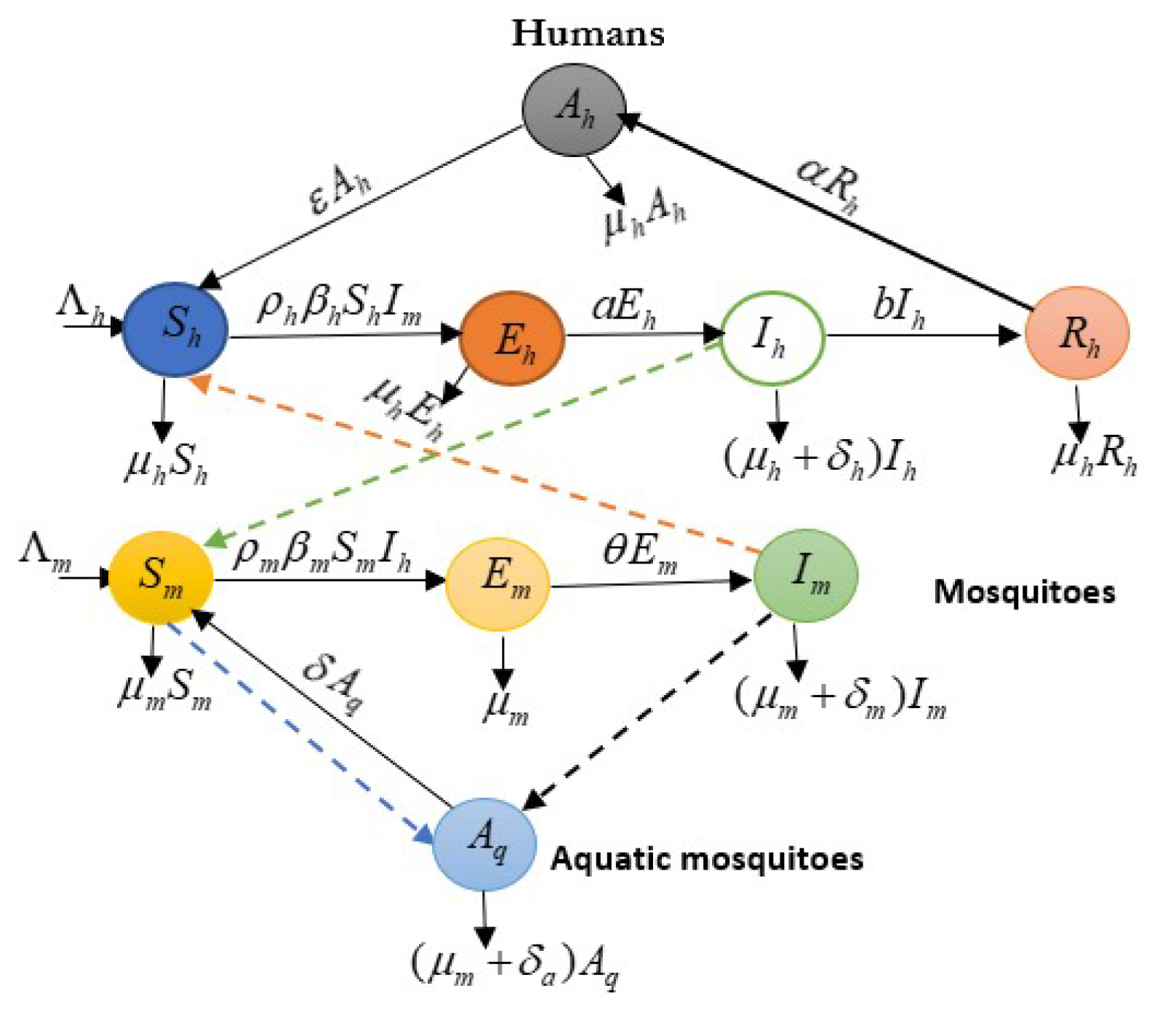

Table 1.
Description of Variables.
| Variables | Biological description |
|---|---|
| The number susceptible humans with time | |
| The number of aware humans with time | |
| The number of exposed humans with time | |
| The infectious humans with time | |
| The recovered humans with time | |
| The number of adult healthy mosquitoes with time | |
| The number of exposed mosquitoes with time | |
| The number of infectious mosquitoes with time | |
| The number of Aquatic mosquitoes (eggs, larvae, pupae) with time |
Table 2.
Description of Parameters.
| Parameters | Biological description |
|---|---|
| Recruitment per-capita rate of susceptible humans | |
| Recruitment per-capital rate of susceptible mosquitoes | |
| Rate of aware human return to susceptible humans | |
| Rate of recovered human become aware humans | |
| Natural death rates of all humans | |
| Natural death rates of all mosquitoes | |
| Transmission rates per-capita of humans | |
| Transmission rates per-capita of mosquitoes | |
| Per- capita contact rates of human with infected mosquitoes | |
| Per- capita contact rates of healthy mosquitoes with infectious humans | |
| a | Rates of exposed human move to infectious humans |
| b | Rate of recovered humans |
| Progression rate of exposed mosquitoes become infectious mosquitoes | |
| Disease induced-mortality rate of infectious human | |
| Proportion rate of the oviposition | |
| Proportion rate of non-infected eggs laid by infected mosquitoes. | |
| Proportion rate in which mosquitoes mature | |
| Mortality rate of infectious mosquitoes due to human activities | |
| Mortality rate of aquatic mosquitoes due to human activities |
2.1. Model Assumption
The model assumes that the mosquito population is homogeneously mixed, meaning that each mosquito has an equal chance of coming into contact with an insecticides. It also presumes that community awareness efforts are uniformly distributed and have a consistent impact on reducing malaria transmission. Furthermore, the model considers environmental factors to be constant over time, allowing for a focus on the interactions between control measures and mosquito behaviour. It assumed that the human and mosquito populations are divided into separate classes, with each distinct one assigned to only one class at a time. In this study, mosquitoes go through an aquatic (water-based) stage before becoming adults with the rate . Only adult mosquitoes are capable of transmitting malaria. It is assumed that malaria spreads through bites?susceptible humans can get infected by bites from infectious mosquitoes, and mosquitoes can become infectious after biting infected humans. Also assumed that the people who recover from malaria may become more aware of the disease and help increase overall community awareness. Therefore, insecticide use increases the death rate of mosquitoes, especially those that are infected. Finally, the community awareness helps reduce the likelihood of people getting infected by promoting protective actions and behaviours.
2.2. Model Description
Susceptible humans ; are humans who have not yet been infected with malaria but are at risk of contracting the disease. These humans are increasing the population through immigration and birth rate. Then decreasing the population through the infectious mosquito rate and the natural death rate of mosquitoes, which gives;
Aware humans ;these population increasing through recovered rate of human and decreasing to susceptible human class. This class are knowledgeable about the life cycle of mosquitoes and the role they play in malaria transmission, thus;
Exposed humans ; are individuals who have been bitten by mosquitoes carrying the malaria parasite but have not yet developed symptoms of the disease. This class increasing through contact rates of human with mosquitoes and decreasing with some rates move to infectious human, gives;
Infectious humans ; play a crucial role in the transmission dynamics of malaria, as they serve as hosts for the malaria parasites. When a mosquito bites an infectious human, it can acquire the parasites, which then develop within the mosquito before being transmitted to other humans, thus;
Recovered human ; a recovered human in this context refers to an individual who has successfully overcome a malaria infection and is now immune to the specific strain they encountered. thus;
Susceptible mosquitoes ; are those that are vulnerable to the effects of insecticides, meaning they can be effectively controlled or eliminated through chemical interventions, gives;
Exposed mosquitoes; are those that have come into contact with insecticides but have not yet succumbed to their effects, thus;
Infectious mosquitoes are produced by the maturation of infected aquatic mosquitoes and the infection of susceptible mosquitoes. thus;
Aquatic mosquitoes ; increasing via oviposition by and infectious mosquitoes at and respectively, where is the oviposition rate while is a proportion of non-infected eggs laid by infected mosquitoes. It decreases through mature mosquitoes at a rate , die naturally at and mortality rate at , thus;
The following non-linear differential equations represent the model description for the transmission of mosquito diseases in the community and correspond to the model diagram in Figure 1, gives;
with the initial conditions;
, and .
2.3. Basic Properties of the Model
The basic properties of the model include the parameters that govern the interaction between mosquitoes and humans, such as transmission rates and insecticide effectiveness. The feasible region defines the set of all possible states of the system, ensuring that population sizes remain non-negative and within biologically realistic limits. The invariant region refers to a subset of the feasible region where the system’s dynamics are constrained to remain over time, reflecting stable population levels and effective malaria control.
2.3.1. Feasible and Invariant Region
The feasible region in this context refers to the set of all possible solutions that satisfy the constraints of the model. Therefore, using the idea of Haile, et al., (2025) in [25] as system (1) will be examined and divided into two, which are both human and mosquito classes, respectively, and given as
Theorem 1.
Let system (1) be the set of then the feasible region Ω contain the all solution.
Proof of Theorem 1.
Suppose , then . To examined the dynamics of system (1), the is positively invariant. This region is determined by considering the entire human population. = Combining the system (1) of the first five equations and differentiating both sides with respect to t yields;
This implies that;
Thus;
Integrating and simplifying both side of equation (3), obtain;
Where is constant value. Using the initial condition, rearrange equation (4), give;
Thus, as , the total human population , which indicates that The invariant region of system (1) for the human population therefore yields:
Thus, is positively invariant. Subsequently, the total population of mosquito in system (1) follow as;
Also, differentiating both side of equation (7) w.r.t, t obtain;
Solving equation (9), gives Hence, the invariant region of system (1) for mosquito population gives;
Therefore, the invariant region of the whole system (1) is given as;
The prove is complete and is positively invariant. Finally, all the solution set of system (1) is bounded in □
2.3.2. Positivity of the Model Solutions
Suppose , for all solution to system (1) with positive initial conditions will stay positive .
Theorem 2.
System (1) can be solved as follows, given positive initial conditions; and with positive initial conditions. Also, and remains positive for all .
Proof of Theorem 2.
Assume that every state variable in system (1) is positive. Starting with (1), the first equation of system (1) is ,
this implies;
Integrating by applying the method of separation of variable along with initial condition, gives;
Also, in the second equation of system (1) as ; this implies;
Integrating the both side and applying initial condition, gives;
The third equation in the system (1) , as , and implies;
Integrating the both side and applying initial condition, gives;
Furthermore, by applying initial condition on all the equations of system (1), obtains;
Thus, the system (1) is mathematically well posed (Hethcote, 2000) in [26]. This complete the prove. □
2.4. Mosquito Disease Free Equilibrium Points
The Mosquito Disease Free Equilibrium Point (DFEP) refers to a state where the mosquito population is present, but there are no cases of the disease being transmitted within the community, meaning . The disease free equilibrium in the system (1) is determined using Maple23 software to identify and set all the model equations to zero.Thus, the disease-free equilibrium point of system (1) is given as . Also, this implies that the disease-free equilibrium is given by;
2.5. Endemic Equilibrium Point
At the endemic equilibrium, the population dynamics of mosquitoes and the incidence of malaria cases reach a steady state. This balance reflects a consistent rate of transmission and infection, where the number of new cases is equal to the number of recoveries or deaths. Modelling this equilibrium is crucial for designing effective control strategies that can reduce the prevalence of malaria in affected communities and is denoted as .
Therefore, EEP are as follows;
2.6. Reproduction Number
The Basic Reproduction Number, often denoted as , is a key epidemiological metric used to describe the contagiousness or transmissibility of infectious agents. It represents the average number of secondary cases generated by one primary case in a completely susceptible population. Understanding helps in assessing the potential spread of malaria and the effectiveness of control measures. The following result is produced by standard method in [27,28].
Considering the infected classes, which are and , gives;
and .
Solving the Jacobian of matrices f and v, then differentiating w.r.t and , gives;
and
.
Subsequently;
Therefore, the basic reproduction number of the model system (1) is denoted by = , where is the spectral radius of the product , which gives;
Where;
.
Therefore, by further simplification, the basic reproduction number , gives;
2.7. Local Stability of Disease Free Equilibrium
The local stability of the disease-free equilibrium is crucial in understanding how effective control measures can be in eradicating malaria. A disease-free equilibrium is stable when the basic reproduction number, , is less than one, indicating that the infection will eventually die out. Mathematical models can help identify conditions under which this stability is achieved, guiding strategies for insecticide use and community education efforts. The following theorem analyses the local stability of DFE.
Theorem 3.
The DFE of system (1), denoted by , is unstable if and locally asymptotically stable (LAS) in Ω if .
Proof of Theorem 3.
At disease-free equilibrium the Jacobian matrix is gives as;
The eigenvalues of the Jacobian matrix are given by finding the characteristic polynomial, which follow as; , obtain;
The focus is on matrix, by considering the rows and columns due to the presence of zeros in the reduction process of equation (29), gives;
The characteristic polynomial of Jacobian matrix in equation (30), is given by;
Where;
Thus, from first expression of equation (31);
and
Subsequently, the second expression of equation (31) can also be in the form of quadratic expression, which is;
Where;
2.8. Global Stability of Disease Free Equilibrium
The global stability of the disease-free equilibrium is crucial for ensuring that malaria transmission can be effectively eradicated. The disease-free state remains stable despite potential perturbations. This involves ensuring the basic reproduction number is less than one, indicating that malaria cannot sustain itself within the community.
Theorem 4.
If , the disease-free equilibrium for system (1) is globally asymptotically stable in the feasible region.
Proof of Theorem 4.
Using the idea of Haile, et al., (2025) in [25] to proof the theorem . The Lyapunov function method is then used to generate an appropriate Lyapunov function following the procedure described in [25]. This will show the global asymptotic stability of the equilibrium point.
Let the Lyapunov function be , where and are non-negative constant and and non-negative infected classes. Then differentiate the Lyapunov w.r.t time, which gives;
Putting the values of and of system (1) to equation (33) by solving it and collecting like terms of the equation, obtain;
.
This implies;
.
Subsequently;
Taking the coefficient of and and obtain;
From the coefficient of , which is , this implies that; . Also, the coefficient of , gives; , and implies that; . The coefficient of , have; , putting in the coefficient of , gives;
and further simplification, resolved as;
Therefore by substituting and equation (35) into equation (34), gives;
Further simplification gives;
Where;
and
Suppose , then;
Thus, if , then . Therefore, . Furthermore, iff , this shows that DFEP,
is globally asymptotically stable (GAS).
Remark 1.If , the disease-free equilibrium is stable and the endemic equilibrium is absent, according to the stability analysis of the reproduction number.
Remark 2.In the event where , the endemic equilibrium may exist and be stable, while the disease-free equilibrium is unstable. Hence the proved.
□
3. Sensitivity Analysis of the Model Using
Sensitivity analysis of the model using the basic reproduction number, , helps identify which parameters most significantly affect the spread of malaria. By analysing how variations in respond to changes in different parameters, researchers can pinpoint key areas for intervention. This information is crucial for optimizing control strategies and improving the effectiveness of insecticide use and community awareness programs.
Sensitivity analysis was used, following the methods described in [32], to ascertain the relative influence of each parameter on the spread of malaria. The normalised forward sensitivity index, as described in [33], is a variable that depends on the differentiable parameter . The analytical outcome of the sensitivity analysis of is obtained by computing to each of the parameters contributing to . Thus, each of the fundamental parameters in has the following sensitivity;
.
3.1. Interpretation of the Sensitivity Index
The sensitivity index provides insight into which parameters have the most significant impact on the model outcomes. By analysing these indexes, researchers can identify which factors most strongly influence mosquito susceptibility to insecticides and the effectiveness of community awareness programs. This understanding helps in prioritising interventions and resources for more effective malaria control strategies. The sensitivity index in Table 3 for shows the expansion of mosquitoes in the community was significantly influenced by the parameters with positive index, which are and . As their values increase, the burden on mosquitoes in the community is reduced by parameters with negative index and .
In order to combat disease in a community, the sensitivity technique showed that public health sectors and non-governmental organisations (NGOs) should use control tactics to decrease positives and improve control of negative index values. The following part examines an optimal control model in light of this observation in order to determine the best strategy for controlling diseases spread by mosquitoes.
4. Optimal Control Technique
The optimal control technique involves using mathematical models to determine the best strategies for managing mosquito populations and reducing malaria transmission. By adjusting variables such as the timing and quantity of insecticide application, this can minimize mosquito resistance while maximizing the effectiveness of control measures. This approach also considers community awareness programs to enhance public participation and improve overall outcomes in malaria prevention [32].
According to [20,34,35], the optimal control model is a powerful mathematical technique that may be used to complex situation analysis. According to [36], the control influences the dynamics of the system by entering the model equations for the ordinary differential equations. The goal is to modify control in order to maximise or minimise a particular functional aim. Similar to this, the problem requires a set of control variables, , a collection of state variables, , and a cost function, , for a time , where and are the beginning and ending times, respectively.
The desired outcome is to determine a control and the related state variables in order to minimise a given objective function. The optimal control approaches in this study focuses as;
- (i)
- : malathion, propoxur and permethrin chemical ingredients,
- (ii)
- : lasting nets insecticides (INI) and
- (iii)
- : traditional techniques.
The non-linear differential equations corresponds to the malaria transmission model diagram in Figure 1 and integrated optimal control technique, gives;
with the initial conditions;
, and .
In order to minimise the cost of control and to determine the optimal control values, equation (39) aims to minimise the total number of exposed individuals, infected individuals, and mosquitoes. of the controls such that the associated state trajectories are optimal control with initially conditions. The following is the objective function;
Subject to (41), where regards as final time and with and are positive weight constants and the choice of this study control agree with the idea in [37,38]. The are the costs associated with the use of malathion, propoxur and permethrin chemical ingredients, lasting nets insecticides (LNI), and traditional techniques. Consequently, the objective function makes it possible to maximise the Hamiltonian related to the optimum control problem. Afterwards, an optimal control , and satisfying equation (39) was obtained using the Pontryagin maximum principle [39];
Where such that are measurable with for is the control set. The controls In [40], are bdd Lebesgue integrable functions? are optimal controls that meet the requirements of Pontryagin’s maximal principle [41]. Equations (39) and (40) are transformed into a pointwise Hamiltonian H minimisation problem using this method, which yields the controls . The Hamiltonian derived from the cost functional of equation (40) and the governing dynamics of equation (39) is used to determine the optimality conditions. Consequently, the following is the Hamiltonian H;
Where are the adjoints that correspond to the state variables. Taking into account, the equation (42) can be solve through appropriate partial derivatives of the Hamiltonian to the associated state variable.
Theorem 5.
Proof of Theorem 5.
The transversality conditions are given as;
According to [39], the integrand of the objective functional is a convex function of and . The system satisfies the Lipshitz property with regard to the variables and and since the solution of (39) is bounded. Consequently, the optimal include exists. By differentiating the Hamiltonian function and evaluating it at the optimal control, the governing equations of the adjoint variables are derived. The adjoint system can therefore be expressed as;
= 1,...,9.
Thus, the result give the control measure as set , which follows with transversality conditions , and the set of control as , gives;
Thus, the arguments, gives;
Therefore;
Furthermore, a sufficient condition for the Hamilton function’s second derivative with respect to . This implies that and This indicates that the optimal problem is minimised at .
Combining the established control set with the initial and transversality conditions allows one to predict the model equations with optimal control strategies in (39) and the adjoint variable as:
This complete the proved. □
5. Optimal Control Simulations of the Model
Optimal control simulations can be used to determine the most effective strategies for applying insecticides while minimising their use. By simulating different control scenarios, researchers can identify the best approach to reduce mosquito populations and interrupt malaria transmission. These simulations help in evaluating the costs, effectiveness, and potential resistance development. The system (1), optimal control technique in (39), adjoint system in (43), transversality boundary conditions, and initial conditions are ,25], ,40], ,25], ,25], ,40], [40] and ,40], while The cost weight constants corresponding to the state variables are assumed to be and the set of adjoints . However, Table 4 contains the parameter values. Optimal control analysis is solved using numerical simulations using MATLABR2023a [40]. Using the fourth-order forward Runge-Kutta method, the equation (39) is solved given the initial values of state variables. The adjoint equations are then solved using the backward fourth-order Runge-Kutta method. [40,41,43]. According to [44] the following optimal strategies for control are used to assess how control measures affect the decreasing trends in malaria infections as;
- (i)
- Strategy A :malathion, propoxur and permethrin chemical ingredients ,
- (ii)
- Strategy B: lasting nets insecticide(LNI) ,
- (iii)
- Strategy C: traditional techniques ,
- (iv)
- Strategy D: combination of and ,
- (v)
- Strategy E: combination of and ,
- (vi)
- Strategy F: combination of and ,
- (vii)
- Strategy G: combination of and .
6. Results and Discussion
The results indicate that implementing optimal insecticide application strategies can significantly reduce mosquito populations while minimising resistance development. Additionally, enhancing community awareness about malaria transmission dynamics leads to more effective control measures and increased participation in prevention efforts. The combination of these strategies creates a synergistic effect, improving overall public health outcomes in malaria-endemic regions. The sensitivity of mosquitoes strains to insecticides and traditional method, was examined. In Figure 2, the combined control result of the investigation showed that mosquitoes revealed no possible resistance to malathion, propoxur and permethrin as in this studied. It was also found that control showed no significant difference on susceptible unaware human, as shown in Figure 3. Subsequently, the result investigation revealed that and was found to be very effective toward mosquitoes in this study and agrees with the studies in [14] that found insecticide and awareness to be very active against the mosquito vector tested. The community awareness on mosquitoes is effective via campaign on mosquitoes to combat malaria, and can be deduced from Figure 4 and Figure 5 of the recovered individuals. Furthermore, the findings shows from Figure 4, Figure 5, Figure 6, Figure 7, Figure 8, Figure 9, Figure 10, Figure 11, Figure 12, Figure 13, Figure 14, Figure 15, Figure 16, Figure 17 and Figure 18 that employed a mathematical model to examine the resistance patterns of mosquitoes to commonly used insecticides, traditional method and evaluated the community’s awareness and practices related to malaria prevention proved to be effective. Based on the findings, it is recommended to implement targeted insecticide rotation strategies to manage resistance in mosquito populations effectively. Additionally, enhancing community education programs about malaria transmission through media campaign can increase awareness and encourage proactive participation in prevention efforts. Collaborative efforts between researchers, public health officials, and local communities are essential for sustainable control and reduction of malaria cases.
Strategy A: . The objective function J is optimised using controls , while and are set to zero in this method. In this case, the aim is to check the contribution of each combination intervention in reducing the mosquitoes and malaria transmission rate in a community. The results are shown in Figure 2, Figure 18 where the combination of (malathion, propoxur, and propoxur) is effective on susceptible,exposed, infected and aquatic mosquitoes, respectively. Also, from Figure 16, it can be deduced that only the insecticide is used on infected mosquitoes and does not work perfectly in reducing the number of vectors. This shows that relying on a single treatment only will not provide effective results. Subsequently, mass awareness and public campaigns on mosquito control are needed. Simply, this is because using insecticides to kill mosquitoes will help in reducing the susceptible. exposed, infected and aquatic mosquito population. As a result, the number of aquatic mosquitoes in the population drops, hence minimising the malaria transmission.
Strategy B: . The objective function J is optimized using this technique using the control , while . The control combination strategies on exposed human in Figure 6 show no significant difference with that of Figure 7, where mosquitoes seem to be difficult to eliminate on the same dynamics in time. But in Figure 9, where as shown, the combination control strategies revealed that lasting net insecticide effective as the number of exposed and infected mosquitoes are decreasing compared to that of aquatic mosquitoes in Figure 17 and Figure 18 due to the activities of humans to eradicate infected mosquitoes in a community through the use of insecticides. In this scenario, from Figure 14 and Figure 16, it can be deduced where mosquitoes seem to be eliminated using one or two interventions. Finally, it is recommended that these three intervention strategies be implemented simultaneously, especially in endemic areas, to effectively control malaria disease.
Strategy C: . Is optimised using the objective function J in this technique, whereas the other controls are set to zero in Figure 13. Also, from Figure 10, the adult mosquitoes seemed to have been eradicated, and the number of susceptible mosquitoes dramatically decreased throughout the first 100 days. Thus, when the single control strategy in Figure 8 with traditional method in Figure 9 is used to combat susceptible mosquitoes, the threat will be lessened compared to when control is not used.
Strategy D: . Is optimised using the objective function J in this technique, while = 0 is set to zero in Figure 6. Also, from Figure 10, the number of recovered human seemed to have been progressed, and the number of exposed mosquitoes dramatically decreased throughout the first 100 days in Figure 14. Thus, when used lasting net insecticide and as combined control strategy in Figure 11, the threat will be lessened compared without control.
Strategy E: combination of . The objective functional J is optimised using this technique, the control measures , and . The strategy’s applications’ outcomes are displayed in Figure 15 and Figure 17, it shows that the mosquito populations of exposed and aquatic are declining as compared to no control.
Strategy F: combination of . The objective functional J is optimised using this technique, the control measures , and . The control applications are displayed in Figure 9 and Figure 11, it shows that the mosquito populations are declining as recovered individuals increasing.
Strategy G: combination of both A, B, and C with . The objective functional J is optimised using this technique, the control measures , and . The strategy’s applications outcomes are displayed in Figure 13 and Figure 17 it shows that the mosquito populations of susceptible, and aquatic are declining as compared to no control. Thus, the intervention technique is successful in reducing the mosquito population in time. Therefore, government decision-makers and all stakeholders are considered in applying all strategies to combat malaria in the specified time. Finally, there is a need to modify insecticide tactics and improve educational initiatives in order to combat the spread of malaria worldwide.
7. Conclusions
In conclusion, mathematical modelling and optimal control strategies play a crucial role in understanding and managing insecticide susceptibility in mosquitoes. By integrating community awareness campaigns about malaria transmission dynamics, this can enhance the effectiveness of control measures and reduce the incidence of malaria. Continued research and collaboration are essential to develop adaptive strategies that cater to evolving challenges in mosquito control and public health education. Finally, It is recommended to enhance community education and awareness programs about the proper use of insecticides to ensure effective mosquito control. Additionally, investing in research to develop new insecticides that mosquitoes have not yet developed resistance to can be beneficial. Collaboration with health organizations can also improve the implementation of optimal control techniques.
Author Contributions
Conceptualization and methodology, Ghaziyah Alsahli; validation, software, Adamu Gambo; formal analysis, Nura Alotaibi; investigation, resources, data curation and writing original draft preparation, Ghaziyah Alsahli; writing review and editing, Adamu Gambo; visualization, supervision, project administration, Nura Alotaibi; funding acquisition, Ghaziyah Alsahli. All authors have read and approved the published version of the paper.
Funding
This work was funded by the Deanship of Graduate studies and scientific research at Jouf University Sakaka, Kingdom of Saudi Arabia under grant No (DGSSR-2025-02-021).
Institutional Review Board Statement
Not applicable for the section.
Informed Consent Statement
Not applicable for the section.
Data Availability Statement
The results of this investigation were supported by hypothetical data, found in the reviewed publications.
Acknowledgments
The authors express their gratitude to Jouf University Sakaka, Kingdom of Saudi Arabia’s Deanship of Graduate Studies and Scientific Research for its assistance.
Conflicts of Interest
The authors declare that there is no evidence of any conflicting financial interests or personal relationships influencing any of the works discussed in this research.
Abbreviations
The following abbreviations are used in this manuscript:
| WHO | World Health Organisation |
| IRS | Indoor residual spraying |
| LNI | Lasting nets insecticide |
| EEP | Endemic equilibrium point |
| Basic reproduction number | |
| DFE | Disease-free equilibrium point |
| GAS | Globally asymptotically stable |
| NGOs | Non-governmental Organisation |
References
- World Health Organization. World malaria report 2023. meeting report, 18–20 April 2023. World Health Organization. https://iris.who.int/handle/10665/374472, 2023.
- World Health Organization. Global technical strategy for malaria 2016-2030. World Health Organization, 2015.
- Fagbohun, I. K. , Idowu, E. T., Otubanjo, O. A. & Awolola, T. S. Susceptibility status of mosquitoes (Diptera:Culicidae) to malathion in Lagos, Nigeria. Animal Res. Int 2020, 17, 3541–3549. [Google Scholar]
- Hussaini, A. , Isaac, C., Rahimat, H., Collins, I., Cedric, O. & Solomon, E. The burden of Bancroftian Filariasis in Nigeria: A review. Eth. J. health sci 2020, 30, 301–310. [Google Scholar]
- Shetty, V. , Sanil, D. & Shetty, N. J. Insecticide susceptibility status in three medically important species of mosquitoes, Anopheles stephensi, Aedes aegypti and Culex quinquefasciatus, from Bruhat Bengaluru Mahanagara Palike, Karnataka, India. Pest manag. sci 2013, 69, 257–267. [Google Scholar] [PubMed]
- Ukpai, O. M. & Ekedo, C. M. Insecticide susceptibility status of Culex quinquefasciatus Diptera: Culicidae in Umudike, Ikwuano LGA Abia State, Nigeria. Int. J. Inno. Scien. Res 2019, 6, 114–118. [Google Scholar]
- Kura, I. S. , Ahmad, H., Olayemi, I. K., Solomon, D., Ahmad, A. H. & Salim, H. The status of knowledge, attitude, and practice in relation to major mosquito borne diseases among community of Niger State, Nigeria. Afri. J. Biomedical Res 2022, 25, 339–343. [Google Scholar]
- Stresman, G. , Whittaker, C., Slater, H. C., Bousema, T., & Cook, J. Quantifying Plasmodium falciparum infections clustering within households to inform household-based intervention strategies for malaria control programs: An observational study and meta-analysis from 41 malaria-endemic countries. PLoS medicine 2020, 17, e1003370. [Google Scholar]
- Sandfort, M., Vantaux, A., Kim, S., Obadia, T., Pepey, A., Gardais, S.,& Mueller, I. Forest malaria in Cambodia: The occupational and spatial clustering of Plasmodium vivax and Plasmodium falciparum infection risk in a cross-sectional survey in Mondulkiri province, Cambodia. Malaria j 2020, 19, 413.
- Hafez, A.M. , & Abbas, N. Insecticide resistance to insect growth regulators, avermectins, spinosyns and diamides in Culex quinquefasciatus in Saudi Arabia. Parasites Vectors 2021, 14, 558. [Google Scholar] [CrossRef]
- Helmi, N. Structure-based virtual screening study for identification of potent insecticides against Anopheles gambiae to combat the malaria. J. vector borne disea 2024, 61, 253–258. [Google Scholar] [CrossRef]
- Naaly, B. Z. , Marijani, T., Isdory, A., & Ndendya, J. Z. Mathematical modeling of the effects of vector control, treatment and mass awareness on the transmission dynamics of dengue fever. Comp. Methods Prog. Biomedicine Update 2024, 6, 100159. [Google Scholar]
- Shittu, R. A. , Thomas, S. M., Roiz, D., Ruiz, S., Figuerola, J., & Beierkuhnlein, C. Modeling the effects of species associations and abiotic parameters on the abundance of mosquito species in a Mediterranean wetland. Wetlands Ecology Manag 2024, 32, 381–395. [Google Scholar]
- Helikumi, M. , Bisaga, T., Makau, K. A., & Mhlanga, A. Modeling the Impact of Human Awareness and Insecticide Use on Malaria Control: A Fractional-Order Approach. Mathematics 2024, 12, 3607. [Google Scholar]
- Mwanga, G. G. Mathematical modelling and optimal control of malaria transmission with antimalarial drug and insecticide resistance. J. Bio. Dynam 2025, 19, 2522345. [Google Scholar] [CrossRef] [PubMed]
- Wako, B. H. , Dawed, M. Y., & Obsu, L. L. Mathematical model analysis of malaria transmission dynamics with induced complications. Scie. Afri 2025, 28, e02635. [Google Scholar]
- Ayalew, A. , Molla, Y., & Woldegbreal, A. Modelling and stability analysis of the dynamics of malaria disease transmission with some control strategies. In Abstract Appl. Analy 2024, 8837744, Wiley. [Google Scholar]
- Opaginni, D. B. , & Durojaye, M. O. Mathematical Modelling and Analysis of Malaria Transmission Dynamics with Early and Late Treatment Interventions. Asian Res. J. Math 2025, 21, 78–98. [Google Scholar]
- Jumai, A. C. , & Achema, K. O. Mathematical Assessment on the Impact of Insecticide Spray on the Dynamics of Malaria Transmission Using Non-Linear Mathematical Model. J. Advanced Sci. Optim. Res 2025, 7, 33–50. [Google Scholar]
- Olaniyi, S. , Falowo, O. D., Oladipo, A. T., Gogovi, G. K., & Sangotola, A. O. Stability analysis of Rift Valley fever transmission model with efficient and cost-effective interventions. Scien. Reports 2025, 15, 14036. [Google Scholar]
- Baroudi, M. , Gourram, H., Alia, M., Labzai, A., & Belam, M. Mathematical modelling and optimal control approaches for dengue. Iranian J. Numer. Analy. Optim 2025, 15, 396–423. [Google Scholar]
- Al Basir, F. , & Abraha, T. Mathematical modelling and optimal control of malaria using awareness-based interventions. Mathematics 2023, 11, 1687. [Google Scholar]
- Arias-Castro, J. H. , Martinez-Romero, H. J., & Vasilieva, O. Biological and chemical control of mosquito population by optimal control approach. Games 2020, 11, 62. [Google Scholar]
- Al-Shanfari, S. , Elmojtaba, I. M., Al-Salti, N., & Al-Shandari, F. Mathematical analysis and optimal control of cholera–malaria co-infection model. Results Cont. Optim 2024, 14, 100393. [Google Scholar]
- Haile, G. T. , Koya, P. R., & Mosisa Legesse, F. Sensitivity analysis of a mathematical model for malaria transmission accounting for infected ignorant humans and relapse dynamics. Frontiers Appl. Math. Stat 2025, 10, 1487291. [Google Scholar]
- Hethcote, H. W. The mathematics of infectious diseases. Socie. Industrial Appl. Math (SIAM) review 2000, 42, 599–653. [Google Scholar] [CrossRef]
- Van den Driessche, P. Reproduction numbers of infectious disease models. Infec. disea. modell 2017, 2, 288–303. [Google Scholar] [CrossRef] [PubMed]
- Van den Driessche, P.; Watmough, J. Reproduction numbers and sub-threshold endemic equilibria for compartmental models of disease transmission. Math. biosci 2002, 180, 29–48. [Google Scholar]
- Brauer, F. , Castillo-Chavez, C., Mubayi, A.,& Towers, S. Some models for epidemics of vector-transmitted diseases. Infec. Disea. Modell 2016, 1, 79–87. [Google Scholar]
- Diekmann, O. , Heesterbeek, J. A. P., & Roberts, M. G. The construction of nextgeneration matrices for compartmental epidemic models. J. Royal Socie. Interface 2010, 7, 873–885. [Google Scholar]
- Murray, J.D. Mathematical Biology I, An introduction, 3rd Ed. Springer-Verlag Berlin Heidelberg, 2001.
- Alemneh, H. T. , & Alemu, N. Y. Mathematical modelling with optimal control analysis of social media addiction. Infec. Disea. Modell 2021, 6, 405–419. [Google Scholar]
- Al-Jiboory, A. K. Adaptive quadrotor control using online dynamic mode decomposition. Euro. J. Cont 2024, 80, 101117. [Google Scholar] [CrossRef]
- Lenhart, S. , & Workman, J. T. Optimal Control Applied to Biological Models, Chapman and Hall/CRC, London, 2007.
- Mahmooee, S. , RabieiMotlagh, O., & Mohammadinejad, H. M. A non-stochastic control method for systems under small random jumps. Sys. Cont. Letters 2025, 199, 106064. [Google Scholar]
- Pinho, M. , Ferreira, M. M. A., & Smirnov, A. Optimal control problem with nonregular mixed constraints via penalty functions. Sys. Cont. Letters 2025, 196, 106010. [Google Scholar]
- Aldila, D. , & Angelina, M. Optimal control problem and backward bifurcation on malaria transmission with vector bias. Heliyon 2021, 7. [Google Scholar] [CrossRef]
- Deressa, C. T. , Mussa, Y. O., Duressa, G. F. Optimal control and sensitivity analysis for transmission dynamics of Coronavirus. Results Phy 2020, 19, 103642. [Google Scholar] [CrossRef]
- Pontryagin, L. S., Boltyanskii, V. G., Gamkrelidze, R. V., Mishchenko, E. F., Trirogoff, K. N., & Neustadt, L. W. LS Pontryagin Selected Works: The Mathematical Theory of Optimal Processes, Routledge, 2018.
- Jaleta, S. F. , Duressa, G. F., & Deressa, C. T. A mathematical modelling and optimal control analysis of the effect of treatment seeking behaviours on the spread of malaria. Front. Frontiers Appl. Math. Sta 2025, 11, 1552384. [Google Scholar] [CrossRef]
- Gernandt, H. , & Schaller, M. Port-hamiltonian structures in infinite-dimensional optimal control: Primal–dual gradient method and control-by-interconnection. Sys. Cont. Letters 2025, 197, 106030. [Google Scholar]
- Kotola, B. S. , Teklu, S. W., & Abebaw, Y. F. Bifurcation optimal control analysis of HIV/AIDS and COVID-19 co-infection model with numericalsimulation. PLoS ONE 2023, 18, e0284759. [Google Scholar] [CrossRef]
- Ouattara, L. , Ouedraogo, D., Diop, O., Guiro, A. Analysis and optimal control of a mathematical model of malaria. Nonlinear Dynam. Sys. Theory 2024, 24. [Google Scholar]
- Saha, A. K. , Saha, S., & Podder, C. N. Optimal control and cost-effectiveness analysis of a fractional order drug-resistant malaria transmission model with recovered carriers. medRxiv 2025. [Google Scholar]
Figure 2.
Graph of susceptible human dynamics shown in time with control .
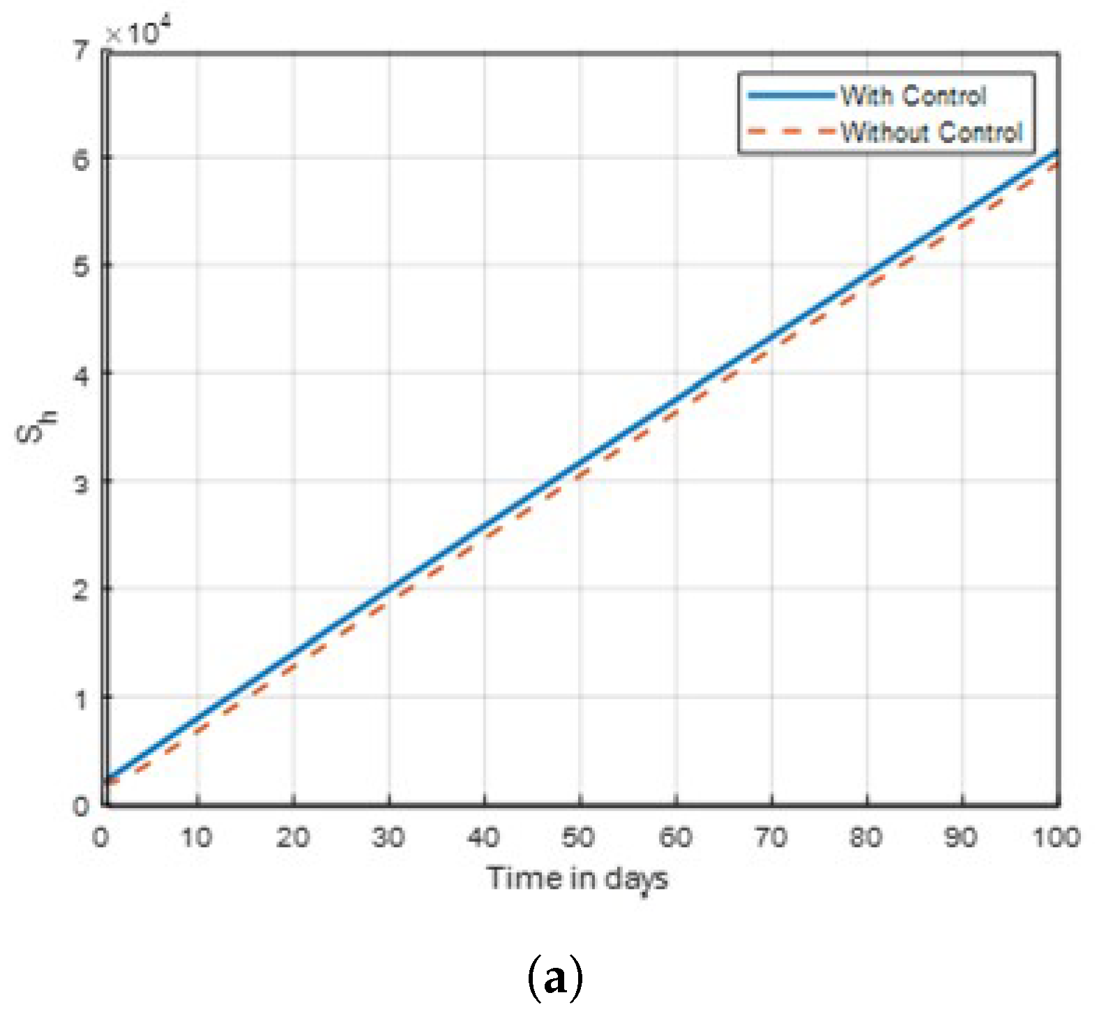
Figure 3.
Graph of susceptible human dynamics shown in time with control combinations .
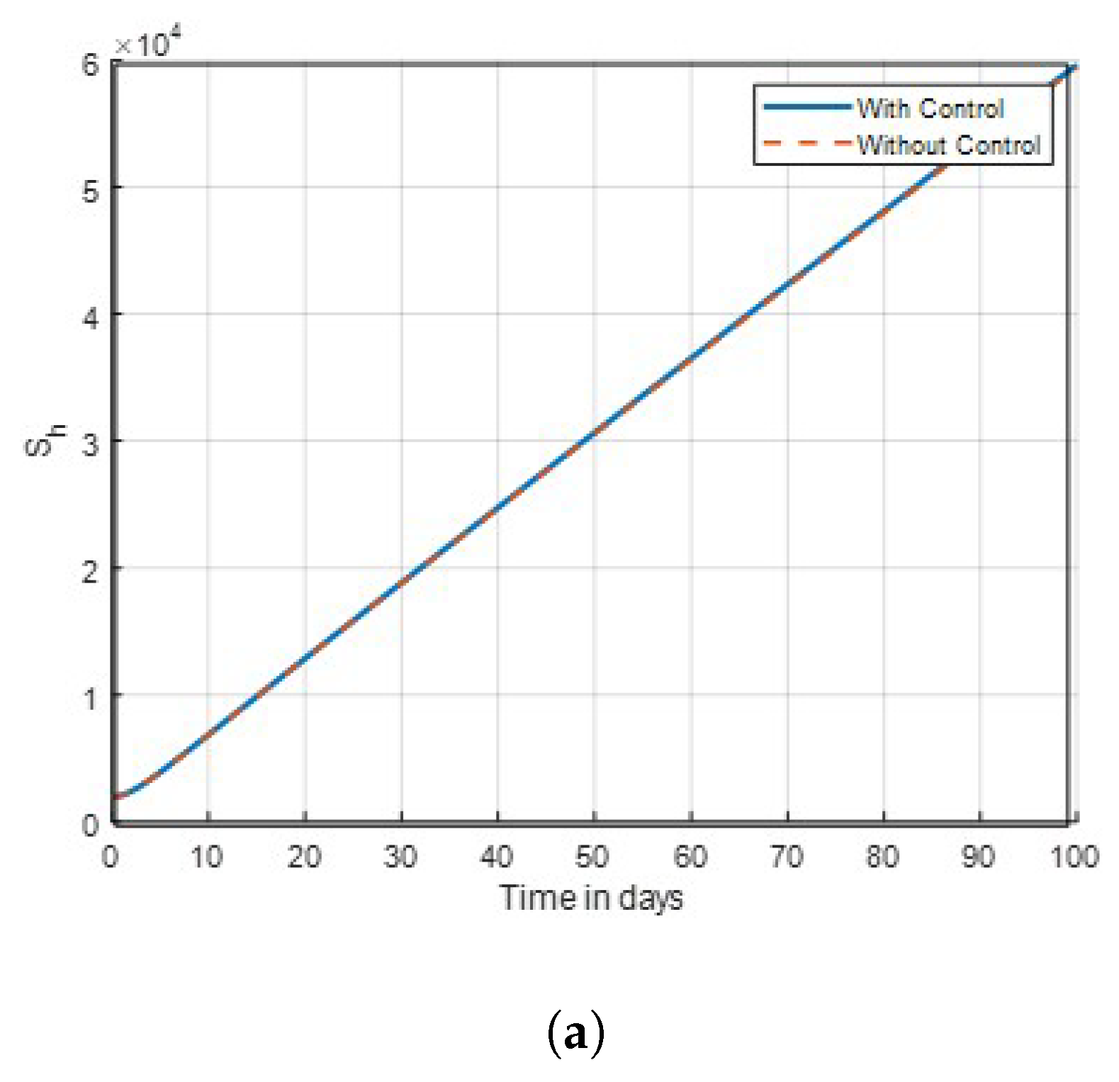
Figure 4.
Graph of aware human dynamics shown in time with varies rates of .
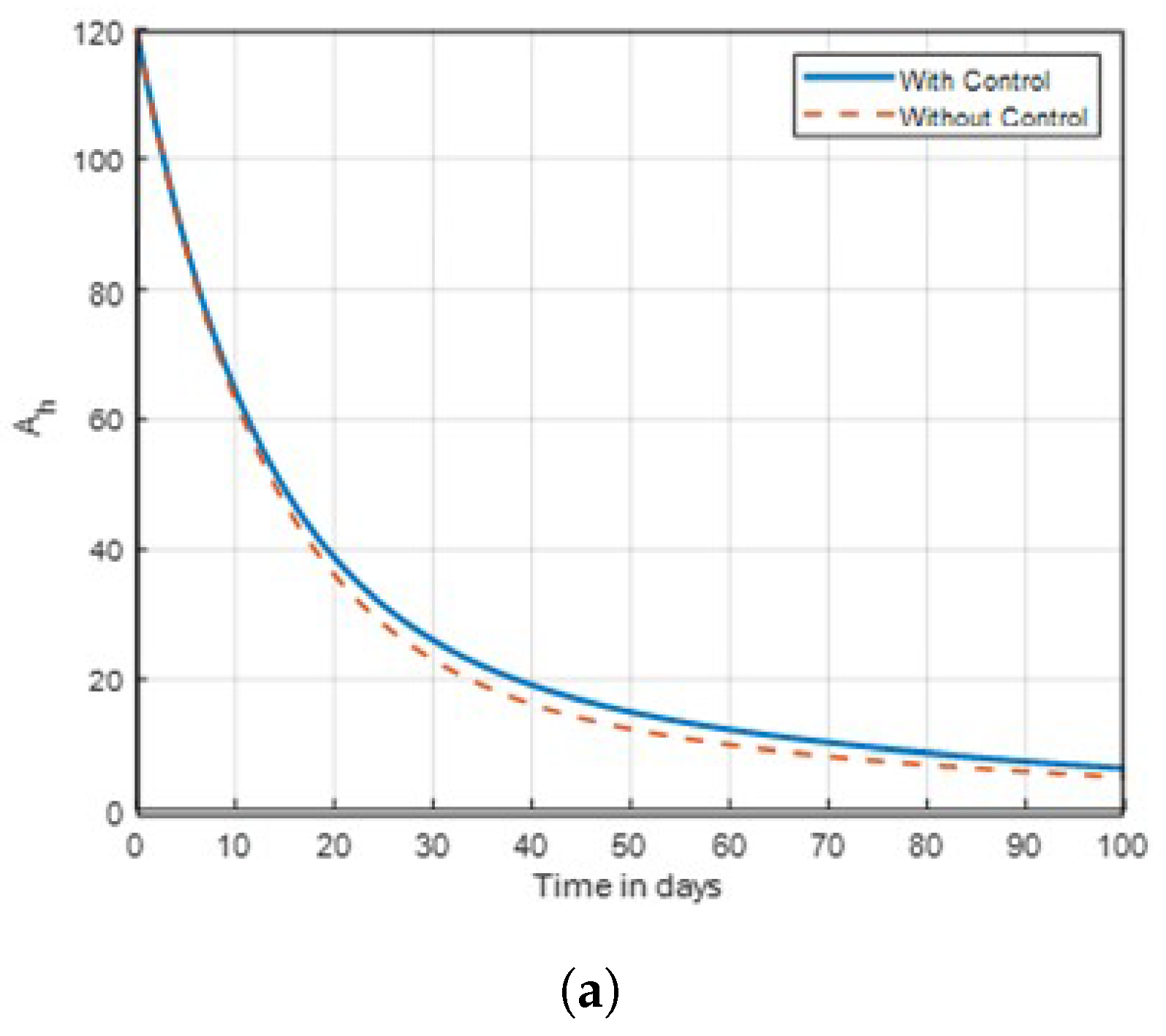
Figure 5.
Graph of aware human dynamics shown in time with varies rates of .
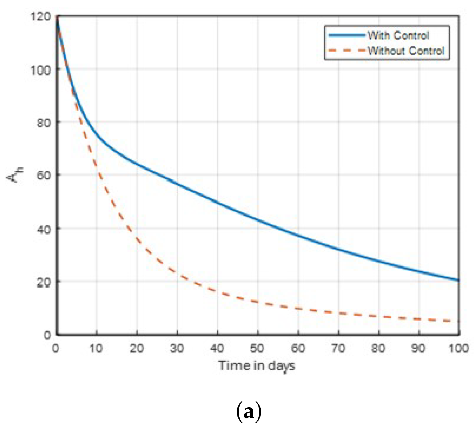
Figure 6.
Graph of exposed human dynamics shown in time with control combinations .
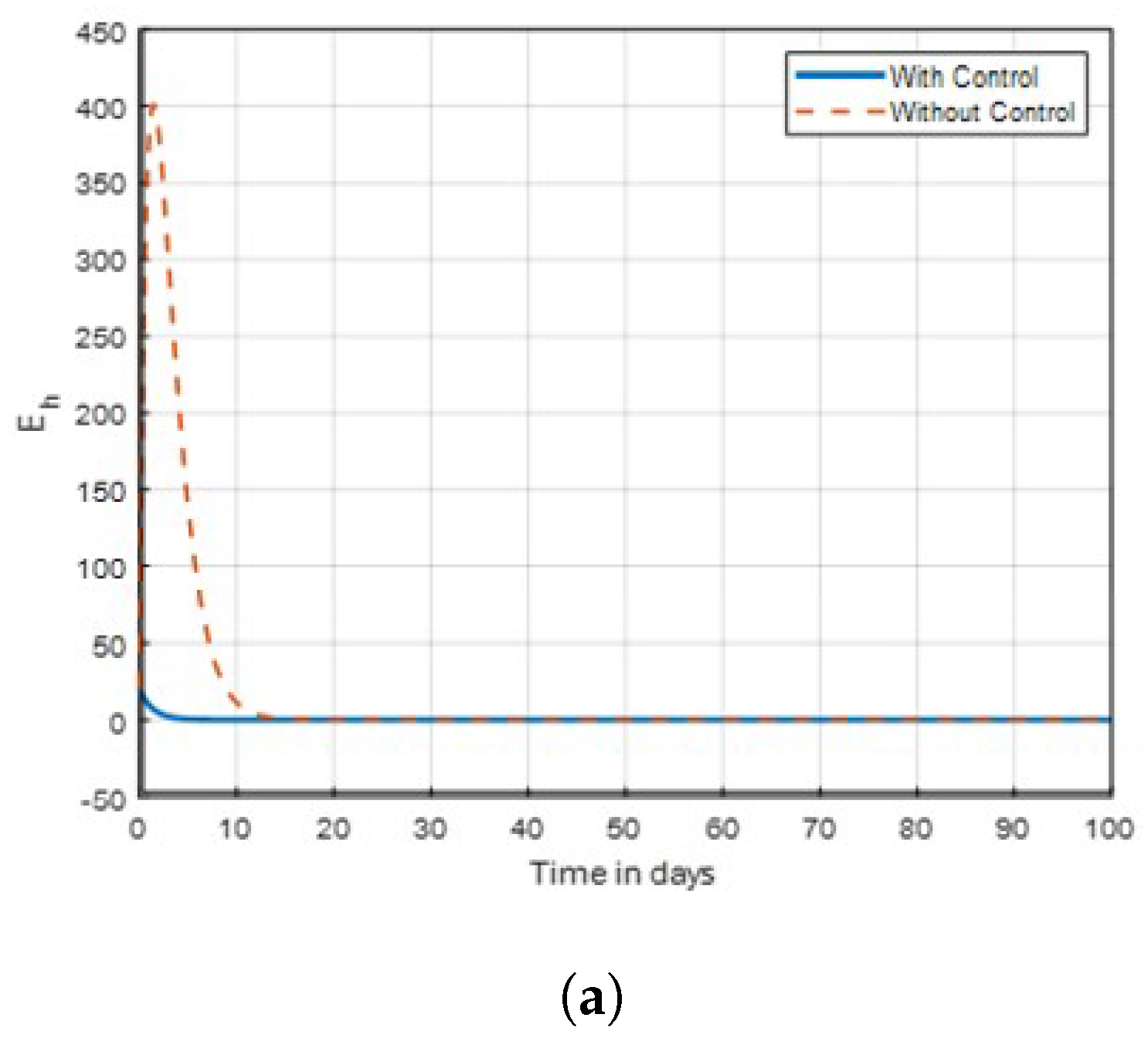
Figure 7.
Graph of exposed human dynamics shown in time with control combinations .
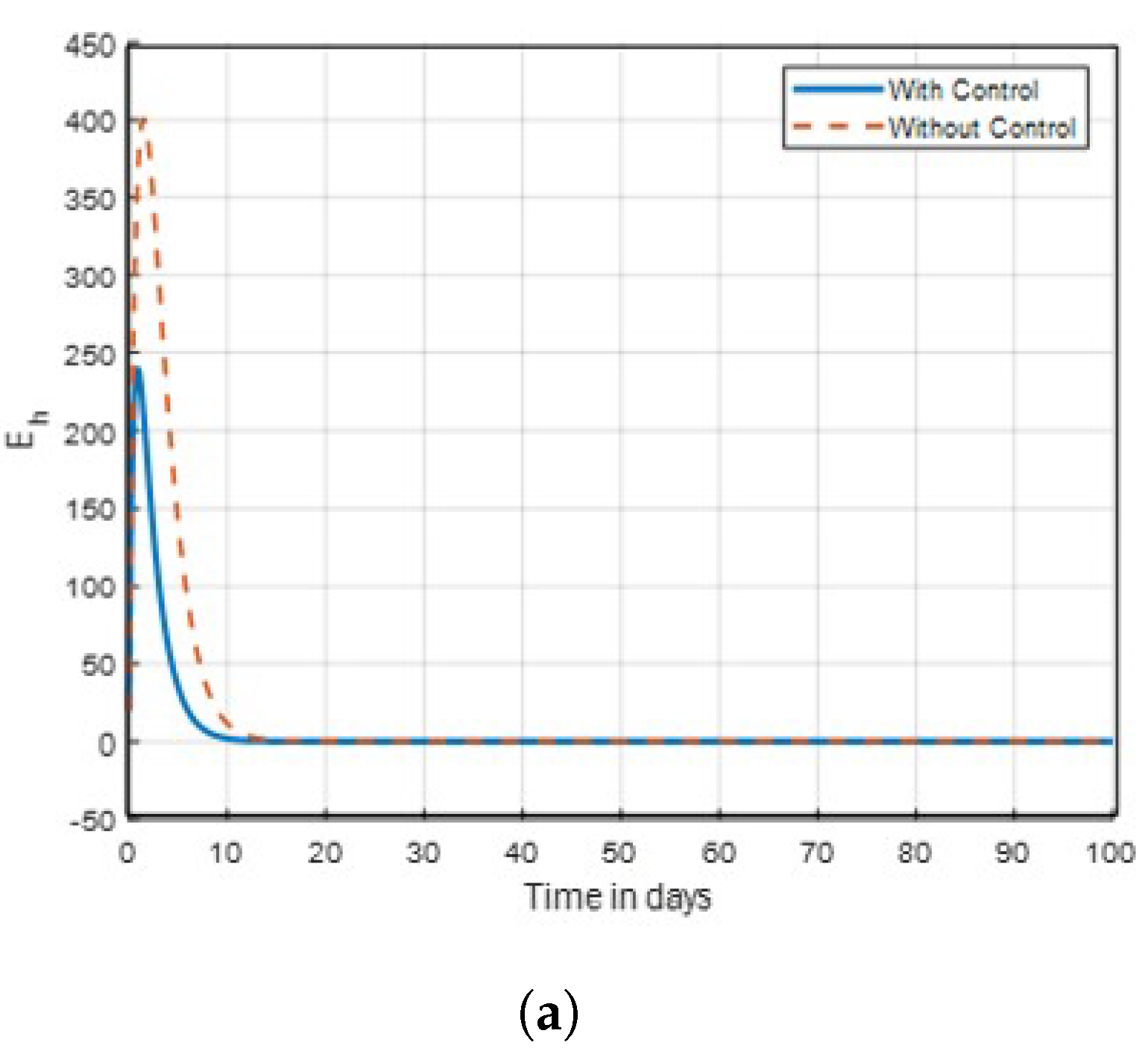
Figure 8.
Graph of infected human dynamics shown in time with control combinations .
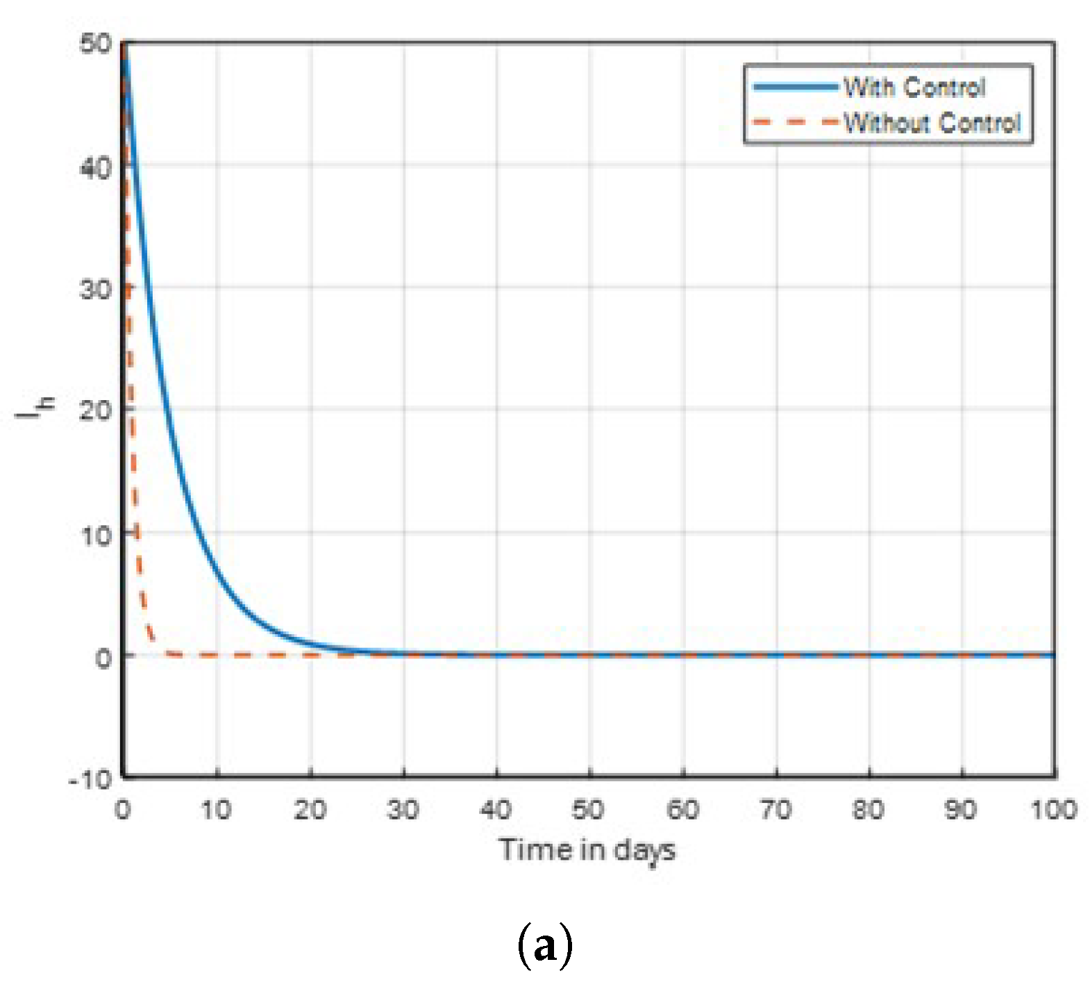
Figure 9.
Graph of infected human dynamics shown in time with control combinations .
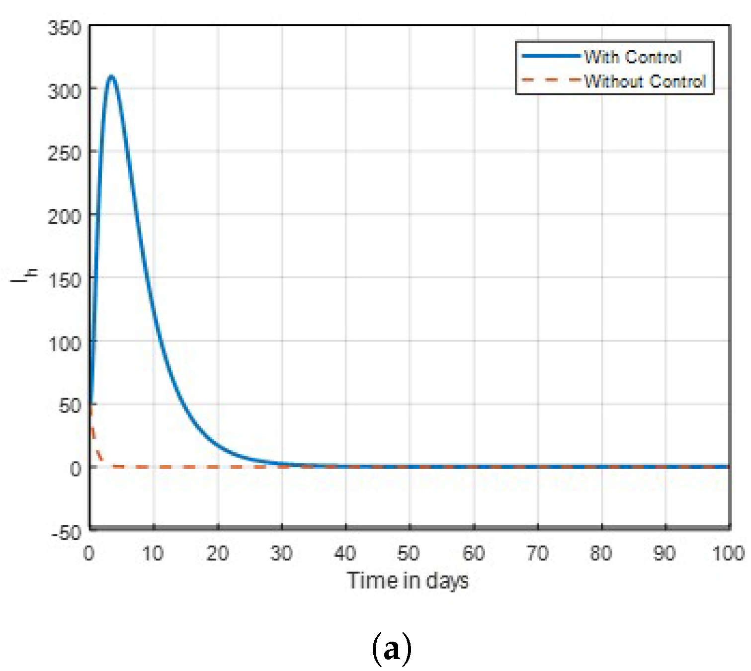
Figure 10.
Graph of recovered human dynamics shown in time with control combinations .
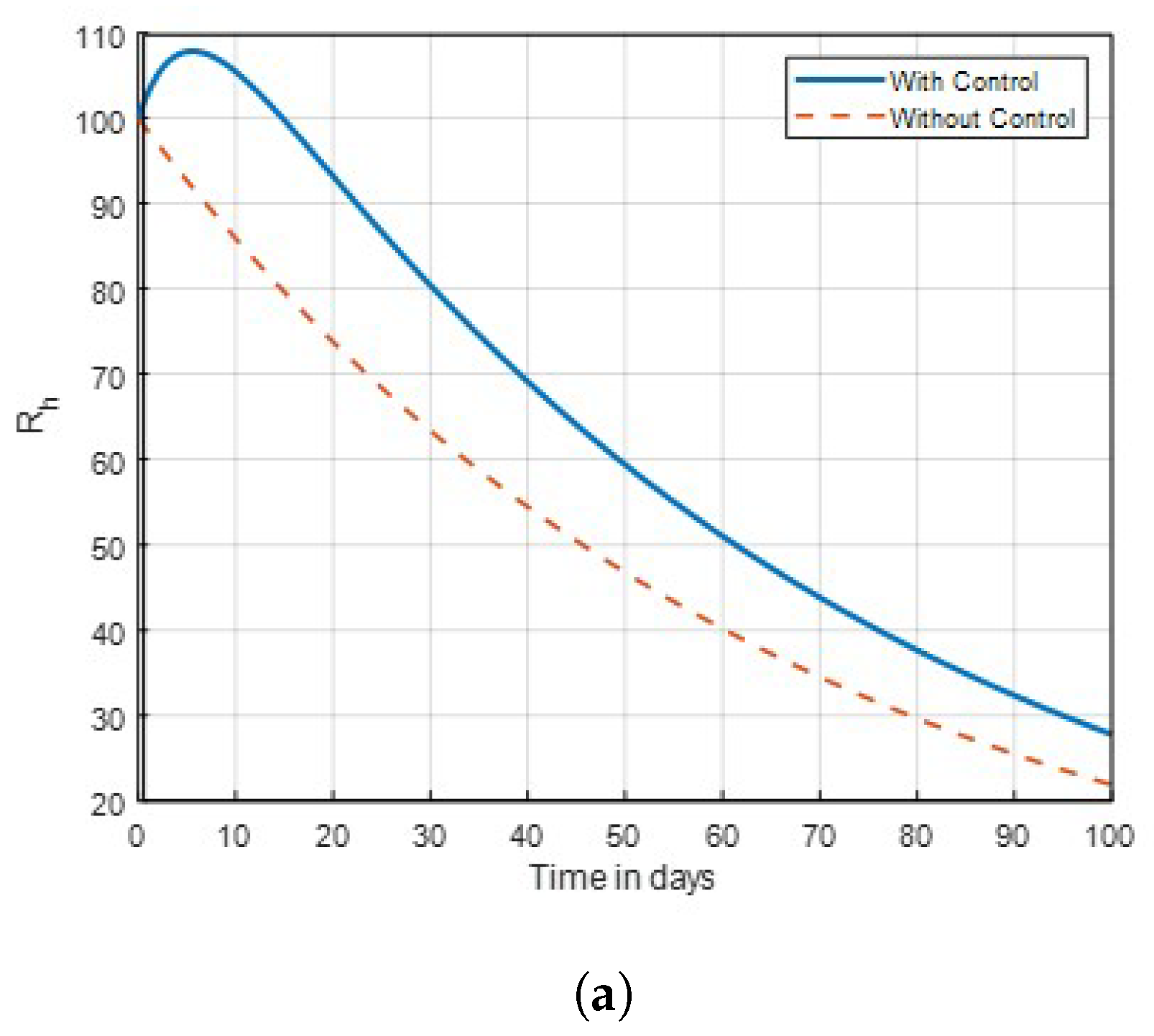
Figure 11.
Graph of recovered human dynamics shown in time with control combinations .
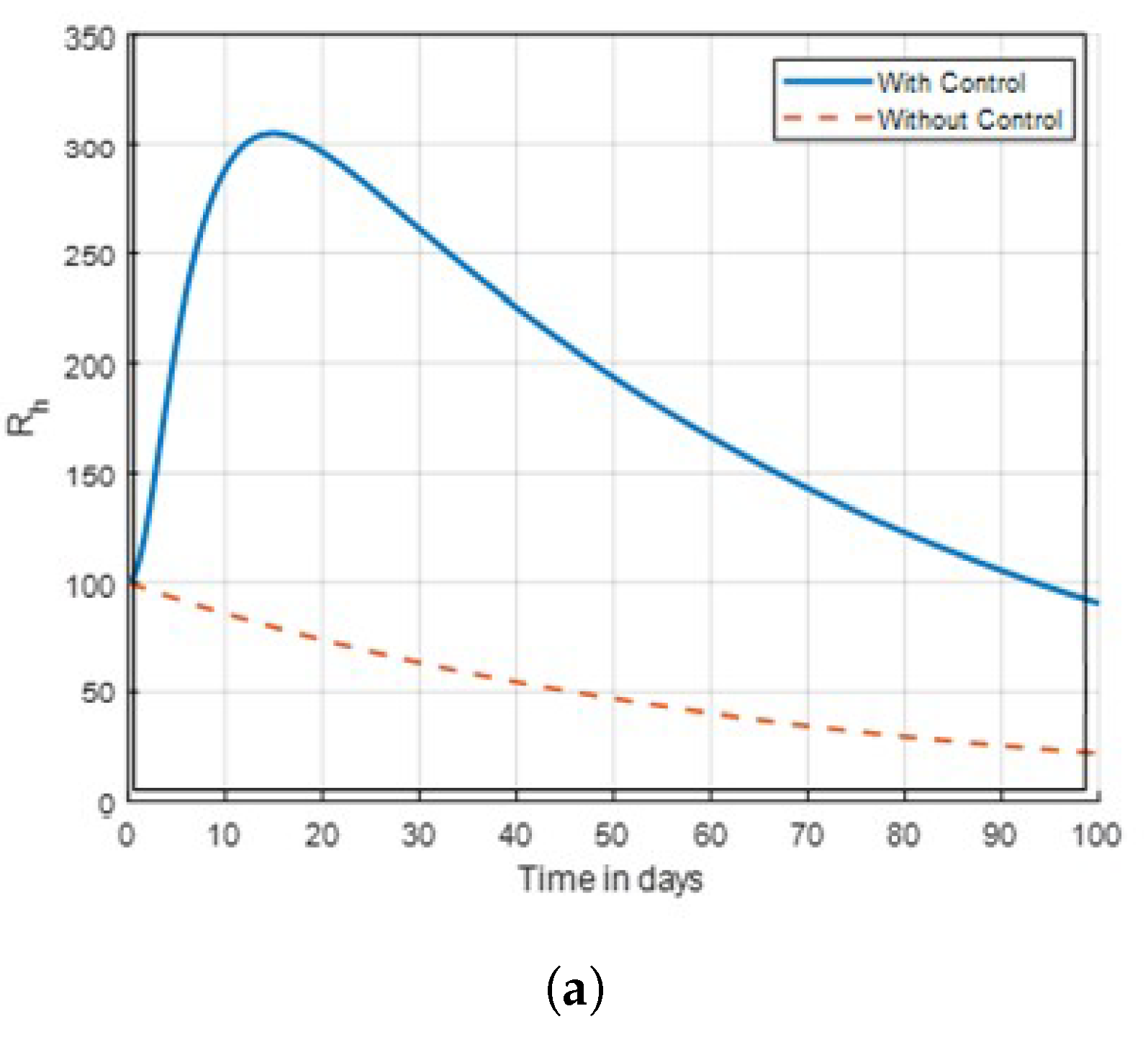
Figure 12.
Graph of susceptible mosquito dynamics shown in time with control combinations .
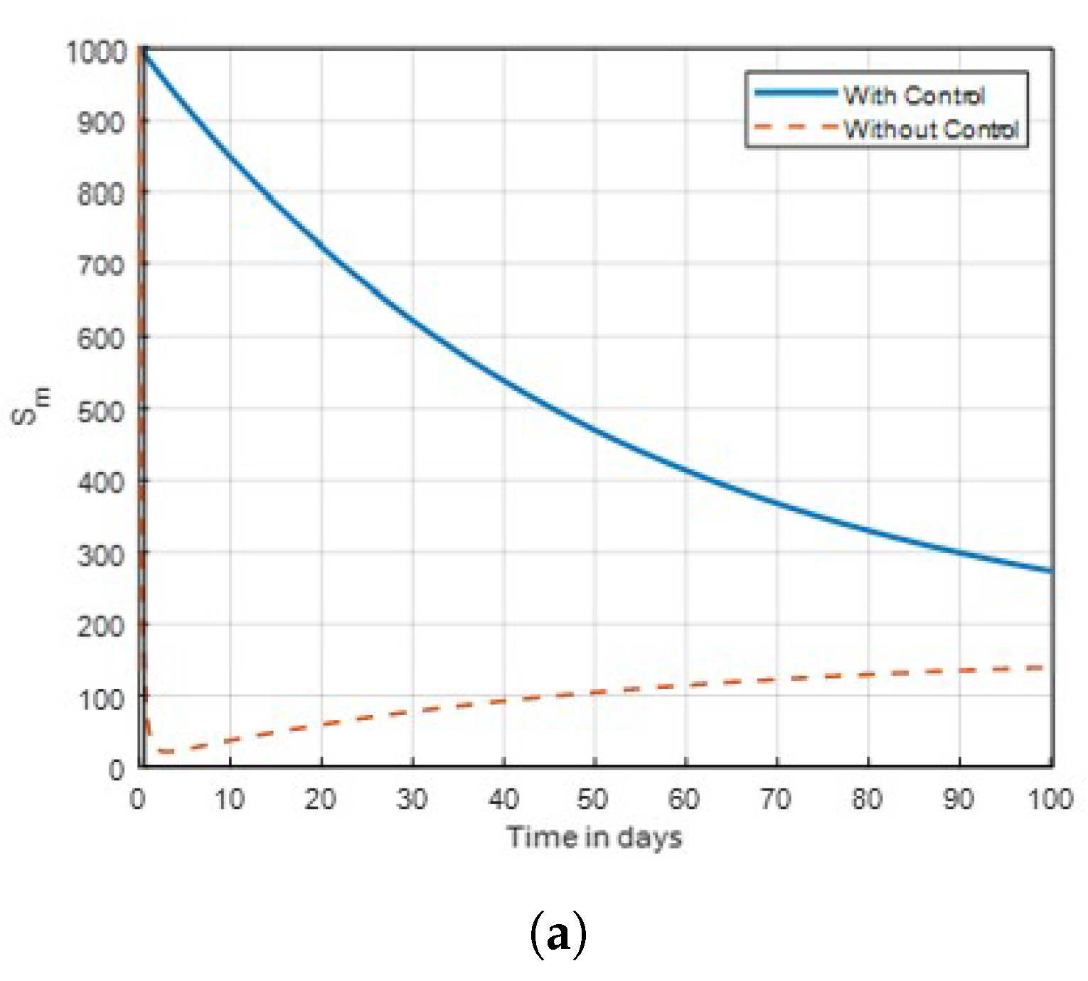
Figure 13.
Graph of susceptible mosquito dynamics shown in time with control combinations .
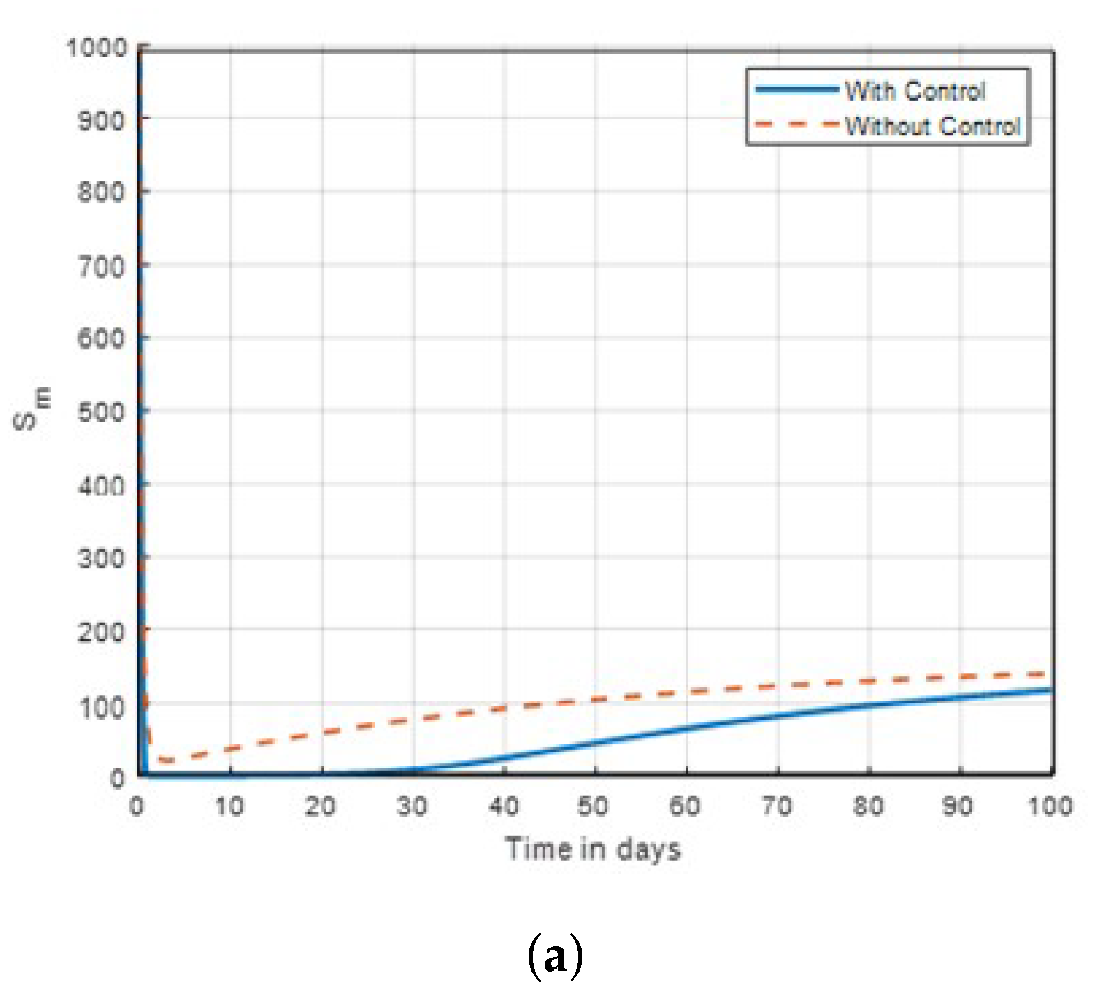
Figure 14.
Graph of exposed mosquito dynamics shown in time with control combinations .
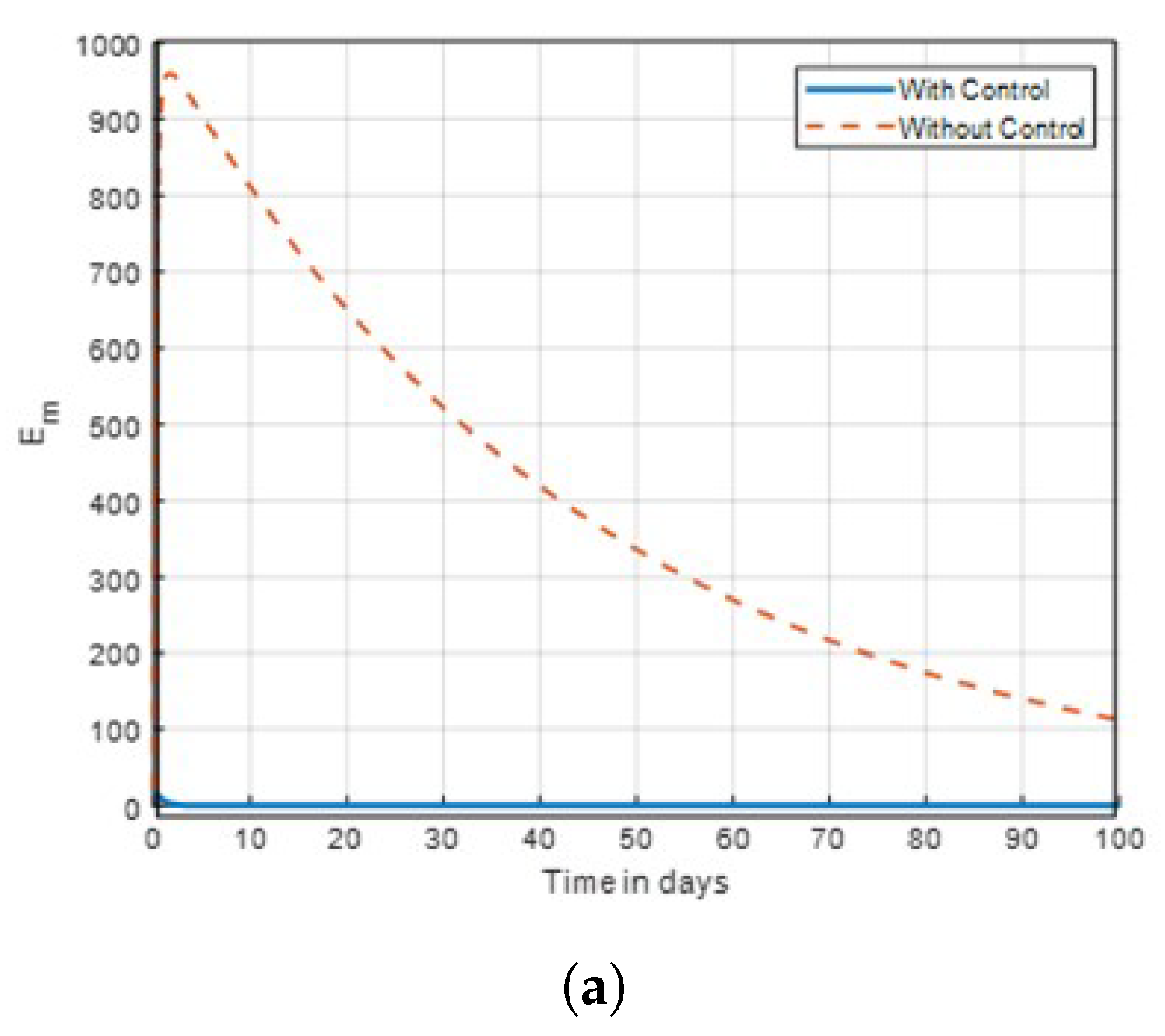
Figure 15.
Graph of exposed mosquito dynamics shown in time with control combinations .
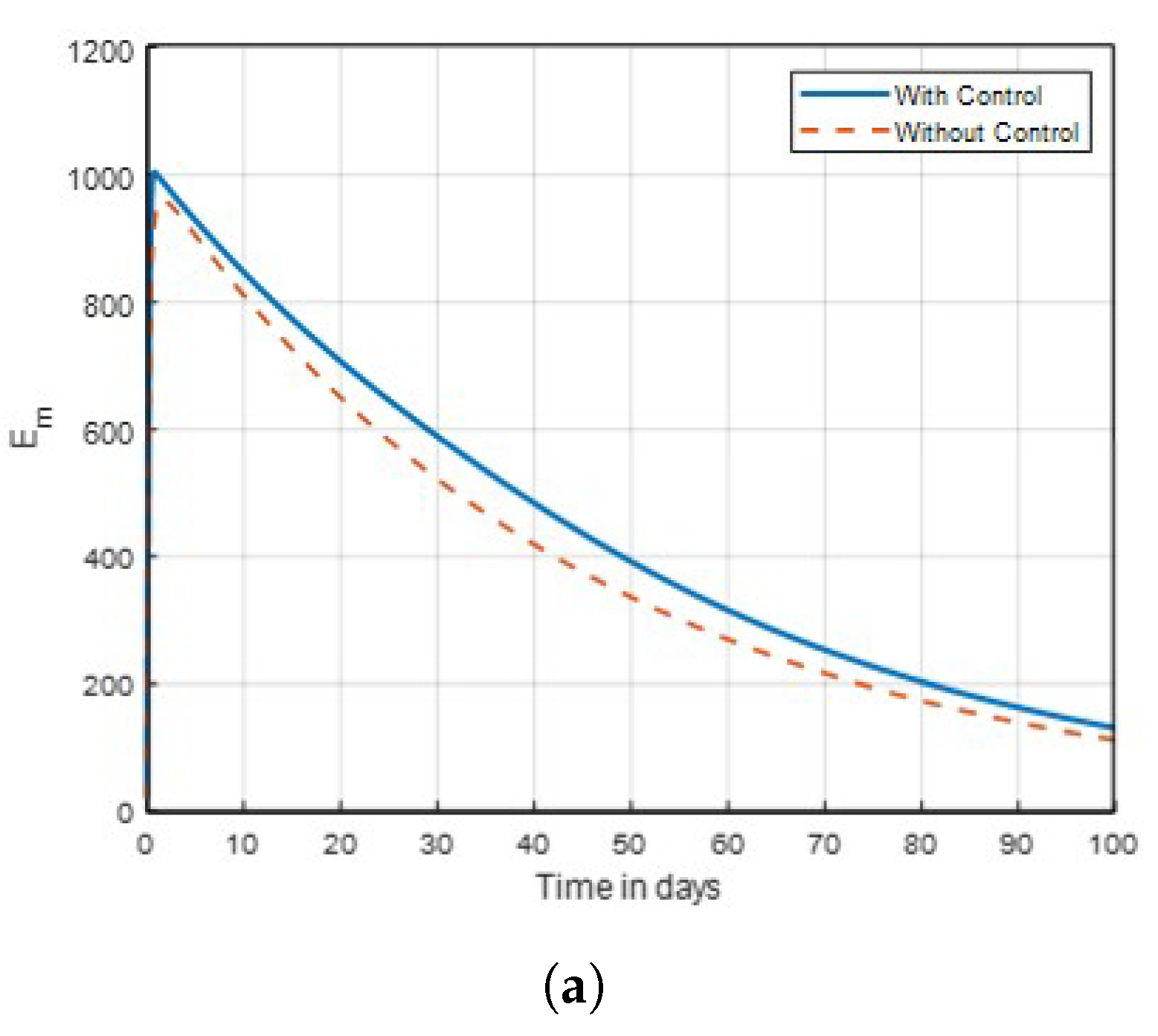
Figure 16.
Graph of infected mosquito dynamics shown in time with control combinations .
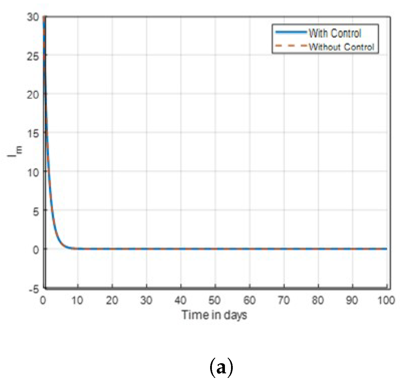
Figure 17.
Graph of aquatic mosquito dynamics shown in time with control combinations .
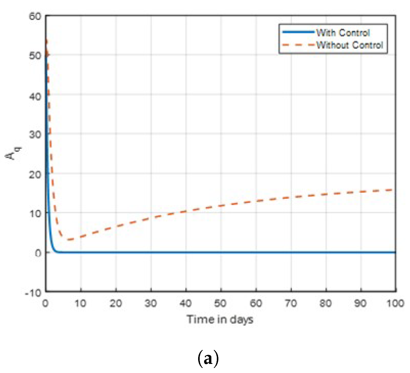
Figure 18.
Graph of aquatic mosquito dynamics shown in time with control combinations .
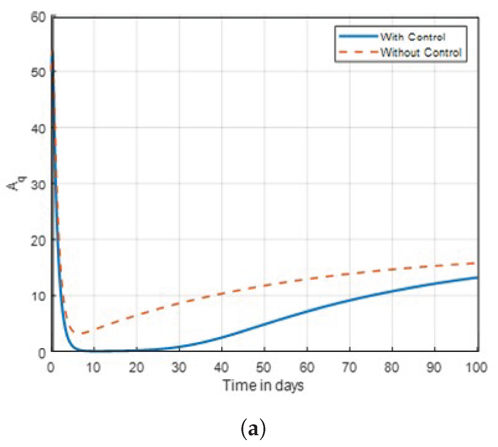
Table 3.
Sensitivity index 0f Parameters of the model.
| Parameters | Parameter value | Sensitivity value | Sensitivity index |
|---|---|---|---|
| 0.041, Estimated | 0.5 | Positive | |
| 220, [25] | 0.5 | Positive | |
| 0.042, [25] | -0.4998702261 | Negative | |
| 0.068, [25] | 0.00004368634364 | Positive | |
| 0.05, Estimated | -0.00007066908525 | Negative | |
| 0.002, Estimated | 0.5 | Positive | |
| 0.00042, Estimated | 0.5 | Positive | |
| 0.0001645, Estimated | 0.4998972084 | Positive | |
| 0.003, Estimated | 0.5 | Positive | |
| a | 0.072, Assumed | 0.5 | Positive |
| 0.00652, [25] | 0.5 | Positive | |
| 0.168, Estimated | -0.0001027913635 | Negative |
Source: Authors.
Table 4.
Parameters of the Model with their Values and Sources.
| Parameters | Parameter value |
|---|---|
| 0.041, Estimated | |
| 220, [25] | |
| 0.042, [25] | |
| 0.068, [25] | |
| 0.05, Estimated | |
| 0.002, Estimated | |
| 0.00042, Estimated | |
| 0.0001645, Estimated | |
| 0.003, Estimated | |
| a | 0.072, Assumed |
| 0.00045, Estimated | |
| 0.001, Assumed | |
| b | 0.1, Assumed |
| 0.0147, Estimated | |
| 0.0018, Estimated | |
| 0.0001, [40] | |
| 0.08, Estimated | |
| 0.00652, [25] | |
| 0.168, Estimated |
Source: Authors.
Disclaimer/Publisher’s Note: The statements, opinions and data contained in all publications are solely those of the individual author(s) and contributor(s) and not of MDPI and/or the editor(s). MDPI and/or the editor(s) disclaim responsibility for any injury to people or property resulting from any ideas, methods, instructions or products referred to in the content. |
© 2025 by the authors. Licensee MDPI, Basel, Switzerland. This article is an open access article distributed under the terms and conditions of the Creative Commons Attribution (CC BY) license (http://creativecommons.org/licenses/by/4.0/).
Copyright: This open access article is published under a Creative Commons CC BY 4.0 license, which permit the free download, distribution, and reuse, provided that the author and preprint are cited in any reuse.


