
Submitted:
04 September 2025
Posted:
05 September 2025
You are already at the latest version
Abstract
The efficient use of solar radiation heat accumulated during the summer months for heating requires the use of high-volume storage tanks. Another option is discharging excess heat outside the system during the summer. This publication concerns the latter solution. A model of the solar heating system for a residential building and pool with a storage tank powered by solar energy has been developed. Simulation calculations were performed, which showed that the removal of excess heat is a beneficial solution, especially when this energy can be used to heat water in the pool. The calculations concerned the heating of a single-family house in a temperate climate. Lowering the temperature of the water in the storage tank contributes to minimal heat losses from the tank to the environment (ground), and supplying the solar collectors with lower-temperature fluid increases the driving force of the heat transfer process.
Keywords:
solar heating
; solar utilizability
; outdoor pool heating
1. Introduction
The use of solar energy is a natural, economical, and environmentally friendly way to maintain adequate thermal comfort in buildings and heat water in swimming pools. One of the problems with solar space heating is the occurrence of excess heat during the summer. To avoid these surpluses, the surface area of the installed collectors should be limited or large-volume heat storage tanks should be used. In the first case, this limits the amount of heat that can be used during the heating season. The large volume of the tanks is also disadvantageous in many respects. In addition to the obvious reasons related to investment costs and location, large tanks have a high external surface area, which means greater heat losses.
In temperate climates, rooms do not require heating during the summer, unlike pools, where heating is often recommended and sometimes even necessary. This is mainly due to the evaporation of water into the environment associated with the high thermal effect of phase change. In addition, the comfortable water temperature in a pool is significantly higher than the air temperature indoors or outdoors. The large mass of water with high heat capacity is also important, as it causes slow direct heating of the water. The solution to the problem of excess heat in storage tanks and heat deficiency in home swimming pools may be the transfer of excess heat from the storage tank to the pool water during the summer.
The use of solar collectors (SCs) for heating has become popular in many countries around the world, including those with cool climates. The simplest method is to store heat in its sensible form, i.e., associated with temperature changes. In this case, water is most often used as the storage medium. Heat can also be stored by utilizing latent heat, which occurs during phase changes of the storage medium. In this case, paraffins or salt hydrates are most often used as the storage medium. Heat can also be stored by utilizing reversible chemical reactions and sorption processes. Sand can also be used as a heat storage material. Sweet and McLeskey presented a study of solar heating of a house with such a heat accumulator in their paper [1]. In contrast, metal was proposed as a heat storage material in the study of Soni et al. [2]. They presented a simulation of the process in which thermal energy was stored in an insulated steel block placed in the ground.
Research on solar space heating most often focuses on the efficiency indicators that can be achieved with given SCs installation parameters in different climatic conditions. Redpath et al. [3] analyzed solar heating of houses in different zones of Europe. They showed that for the Mediterranean zone, seasonal thermal energy storage can fully cover the thermal energy demand of a typical house. However, for the Atlantic and continental climate zones, full coverage is only possible for passive houses, i.e., those with an annual energy demand of less than 15 kWh/m2. Clarke et al. in manuscript [4] studied the influence of the solar collectors’ area Ac and storage tank volume V on system efficiency. The simulation was carried out for a passive house in Ireland. The usable floor area of the house was 215 m2, Ac was 10.6 m2, and V was 23 m3. It was shown that increasing Ac to 20 m2 raise the solar fraction SF from 0.47 to 0.63.
The paper by Antodianis and Martinopoulos [5] has analyzed the impact of V and other solar heating parameters on the SF. The simulations were done for a single-family house in Greece with an area of 120 m2. The SF values ranged from 0.39 to 0.67. Villasmil et al. [6] conducted an analysis of solar heating in residential buildings. The calculations took into account thermal stratification in the tank, and the stratification model used was verified in a large-scale research installation. Meister and Beausoleil-Morrison [7] found that the system under study could achieve a 100% SF for space heating and 86% for domestic hot water loads. Brites et al. [8] presented research on solar heating in warm climates (Portugal). It was found that with a Ac of 10 m2 and V equal to 30 m3, SF = 1 could be achieved for heating.
In the study [9], the authors of this paper conducted simulation studies of solar space heating in temperate climate conditions. The influence of Ac, V, and excess heat removal outside the installation on the SF was investigated. The influence of solar collectors’ inclination angle on the efficiency of solar space heating was presented in [10].
Heating swimming pools has been a challenge for centuries; Roman records show that solar energy was used to warm water in public baths as early as 200 BCE [11]. There has always been a consistent demand for maintaining comfortable water temperatures in both residential and public pools. Among the most commonly used pool heating methods are water heaters powered by fossil fuels, such as diesel, liquefied petroleum gas, and natural gas. However, burning these fuels releases greenhouse gases, which are a major contributor to climate change. Additionally, fossil fuel prices have risen significantly in recent years. These factors have opened the door to the adoption of renewable energy technologies. Currently, there are many publications in the literature discussing this topic. The study [12] presented a method for evaluating energy savings achieved by flat plate SCs assisted heat pumps for heating swimming pool water. Chow et al. [13] analyzed the performance of a solar-assisted heat pump system for indoor swimming pool water and space heating under the subtropical climatic condition of Hong Kong. Ilgaz and Yumrutaş [14] presented a case study on the heating performance of a system combining a solar-assisted heat pump with an underground thermal energy storage tank for swimming pool applications under real climatic conditions in Gaziantep Province, Turkey. The developed analytical model was used to evaluate different performance parameters of the system. A comprehensive state-of-the-art review of swimming pool advanced heating technologies has been presented by Li et al. in [15]. This review covered various systems, including conventional boilers, heat pumps, solar thermal systems, passive and active technologies and hybrid solutions, evaluating their energy efficiency, environmental impact, and economic performance. In the article [11], a mathematical model of an outdoor swimming pool solar heating system in warm climates was developed using TRNSYS application. It has been validated using data collected from an outdoor pool. Zhao et al. [16] presented the flow rate optimization for a pool heating system with SCs. The studies [17,18] investigated the optimal design and impact of heat loss from a storage tank with phase change material on the energy, economic, environmental, and technical performance of a solar-assisted heat pump system for a swimming pool. The usefulness of multi-objective optimization for the design process of different configurations of outdoor swimming pool heating systems with SCs and heat pumps was presented in [19]. The optimization results demonstrated that solar-assisted configurations provide significant improvements in system performance for locations under consideration.
Analysis of swimming pool solar heating using the utilizability method was discussed in article [20] by Gonçalves et al. This approach allows for evaluating solar energy contribution under varying climatic and operational conditions. The study demonstrates that the utilizability method is an effective tool for optimizing solar thermal system design and predicting energy savings in pool heating applications. The simulations were carried out for various locations in Brazil. SF were determined under the following conditions: pool surface area = 250 m2, Ac equal to 150 m2, water temperature 30 °C. For the warmest location among those studied, Fortaleza (3.76°S), SF = 0.69 was determined, while for the coldest, Porto Alegre (30.02°S), SF was equal to 0.21.
The article [21] reviewed recent developments in solar water heaters and collectors, with relevance to applications such as swimming pool heating. It discussed advances in SCs technologies, materials, and system designs that enhance thermal efficiency and durability in pool heating systems. The review emphasizes the growing role of solar thermal solutions in reducing energy consumption and operating costs for swimming pool facilities. The article by Olczak et al. [22] presented a case study comparing the solar energy gain effectiveness of flat plate and evacuated tube SCs in two swimming pool installations located in Poland. The study analyses thermal performance under real operating conditions in a temperate climate, focusing on efficiency, temperature stability, and seasonal variability.
This paper considers solar heating of a single-family house in a temperate climate with accompanying heat transfer (e.g., to a swimming pool) during the summer. The heat flows between the individual components of the system were analyzed. Particular attention was paid to the impact of excess heat discharge to the pool on the SF of the building heating system. A model of the solar heating process for space and pool heating from a storage tank loaded by SCs was developed. Conducted simulation calculations showed that the transferring of excess heat is a beneficial solution. However, this requires the ability to use excess heat, and it is particularly advantageous to use it to heat water in a pool. The calculations for the space heating system in a temperate climate were carried out applying the concept of solar utilizability. The algorithm presented in the authors' earlier work [9] was used as a basis.
2. Solar Radiation
Daily radiation outside the atmosphere is a quantity dependent on the day of the year n, latitude ψ and solar declination δ. The relationship for determining it is as follows:
where 1367 W/m2 is the solar constant (radiation flux density). The solar declination for the n-th day of the year is:
The value is the daily average beam radiation on the tilted surface compared to that on a horizontal surface, which is calculated using the following formula:
The sunset hour angle was determined from:
whereas the sunset hourly angle for an inclined surface :
The dependence on radiation on an inclined surface consists of three components relating to direct, scattered, and reflected radiation, respectively. The component concerning scattered radiation , is characterized by the ratio , which depends on the clearness index . The dependence is empirical and has the form:
The coefficient is defined as follows:
It is assumed that the SCs are located at latitude ψ, face true south, and are tilted at an angle β to the horizon. The basis for determining the daily solar radiation incident on a tilted surface is the radiation values on the horizontal surface . The ratio of these values (daily average total radiation on the tilted surface to that on a horizontal surface) is calculated using the formula:
therefore:
3. Solar System Model
A simplified diagram of the considered solar system consisting of SCs, a hot water storage tank, a heat exchanger for space heating, and a heat exchanger for pool heating is shown in Figure 1. The diagram does not present pumps, valves, or an additional heater in the building. There are two types of solar gains in the installation: direct gain absorbed by the water in the pool and indirect gain absorbed by the water in the tank through the SCs. The heat exchanger in the building operates only during the heating season, while the pool heat exchanger operates during the summer.
The visualization of solar radiation energy flowing through the system under consideration is presented in the Sankey diagram (Figure 2).
The amount of useful energy generated in the collector during a 24-hour period and delivered to the tank is described by the following equation:
where is the collector heat removal factor, is the effective transmittance–absorptance product, is the daily radiation on a tilted collector surface and is daily utilizability. Heat losses from the tank to the surroundings are:
where is the overall heat transfer coefficient of the tank, is the tank surface, is the water temperature in tank, is tank surroundings temperature, and is a time step.
To determine daily heat transferred from the tank to the radiator in the building , two quantities should be considered: the amount of heat that can potentially be transferred to the radiator during the day and the amount of heat that should be transferred to the radiator during the day to maintain the desired room temperature in the building (in winter conditions). The heat transfer equation for is as follows:
where is the mass flow rate in the building circuit, is the heat capacity, is the effectiveness of the heat exchanger, and is the inlet water temperature.
The daily heat required to heat a room is calculated as the multiplication of the overall heat transfer coefficient of the whole building , the building envelope area Aw, and monthly heating degree days :
Heat is equal to the smaller value of and and is transferred to the building only during the heating season [9,23]:
The limits of the heating period can be determined based on the average temperature of the building walls , where is the air temperature.
The daily amount of excess heat transferred to the pool is limited by the pool heat exchanger and is determined from:
where is the mass flow rate in the pool circuit, is the effectiveness of the pool heat exchanger, and is the pool water temperature.
It was assumed that simultaneous heating of the pool water and the building rooms was not possible. Switching the water flow from one place to another depends on the relationship between the temperature of the building walls and the critical temperature, equal to 14 . This is explained in the block diagram shown in Figure 3.
The calculation algorithm is based on the heat balance of the tank, which is supplied with heat in the amount of . The individual components of heat lost by the tank are , , and . The last item in the balance is the heat accumulated in the walls of the building . This amount of heat is described by the following equation:
where is the mass of building, is the heat capacity of walls, and is the wall temperature in the previous time interval.
The thermal balance of the tank in the solar system is as follows:
where is the daily variations of the water temperature in the tank. A detailed description of this algorithm is given in article [9].
The basic indicators determined in this article are SF and solar efficiency SE. SF is the ratio of solar energy delivered to the radiator to the energy required to heat the building :
whereby the summation is performed for individual days of the year. On the other hand, solar efficiency SE is the ratio of the sum and to the amount of solar energy falling on the collectors:
4. Heating Water in an Outdoor Pool
The water in an outdoor pool is exposed to thermal interaction with the atmosphere, which often makes it necessary to heat it in order to maintain comfortable temperatures in the range of 25-30 °C. Figure 4 presents the heat transfer between the water in the pool and the environment. Heat transfer is generated by solar radiation flux, long-wave radiation flux, convective flux, and evaporation flux. These “natural” fluxes are supplemented by heat transfer from the heating system. The assumption was made that the water in the pool has a uniform temperature (it is completely mixed).
The relationships between the individual heat fluxes are presented below. The solar radiation flux is the ratio of daily insolation on a horizontal surface H and the time interval Δt. Long-wave radiation LW is emitted in the opposite direction to solar radiation, i.e. from the water surface to the sky. Flux LW between the water surface and the sky is calculated using the Stefan-Boltzmann equation:
where is the Stefan-Boltzmann constant and is the temperature of the sky.
depends on the air temperature and humidity RH. According to ASHRAE [24], it can be calculated using the following formula:
where in this equation is in K.
Convective flux results from the difference between and and, unlike other fluxes, can be absorbed or released by water. The heat transfer equation determines :
The heat transfer coefficient between the environment and the water surface depends on the hydrodynamic conditions at the water surface. For a known wind speed , can be calculated according to the following equation:
In addition to convective and radiative fluxes, pool loses heat due to water evaporation into the environment. The partial pressure of water vapor at the water surface is generally greater than the partial pressure of vapor in atmospheric air. This difference is the driving force behind the transfer of water from its surface to the environment. The evaporative heat flux EV is given by the relationship:
This relationship, together with the definition of the constant A, is explained in Appendix A.
The heat balance of the water in the pool is as follows. The amount of heat supplied to the water in the pool during the day includes reaching solar radiation and :
where is daily insolation on the horizontal surface. On the other hand, the water in the pool loses heat flux through LW, EV and . The value of depends on the surface area of the water in the pool and the time interval Δt under consideration:
The daily change in the internal energy of the pool water causes a change in water temperature :
According to the law of conservation of energy, the following applies:
5. Results
The calculations were performed using a modified algorithm described in the authors' paper [9]. The modification regarding switching the water flow from the tank-radiator circuit to the tank-pool exchanger circuit was schematically presented in Figure 3. The appropriate calculations were performed for different values of Ac, Ap, V and . The latter value directly determines .
The main purpose of the calculations was to determine whether redirecting the heat outside the space heating system affects the efficiency of space heating system during the heating season. In addition, the relationships between heat flows and temperatures in the solar system are presented.
Due to the large number of parameters in the simulated process, the values of some of them were set at a constant level. A summary of their values is shown in the Table 1.
5.1. Climate Parameters
For the location considered in this study (Krakow, Poland), Figure 5 shows the average for individual days of the year generated from data taken from Photovoltaic Geographical Information System (PVGIS) [27]. This relationship was approximated by a periodic function (a). After converting the daily average data to monthly averages, a function was created to approximate these data as well. Its mathematical form (b) and graphical representation are almost identical to those for the daily average data.
It has been assumed that the heating season is the period during which the average daily air temperature is below 14 °C. This corresponds to the period from day 260 to day 134 of the following year.
For the calculation of H, hourly insolation data obtained from the PVGIS database [27] were used. These data were converted to daily and then to monthly average daily values, and an approximation function (c) presented in Figure 6 was created based on them. This figure shows the values H for individual days of the year for the location under consideration, i.e. Krakow. In Figure 6, the course of the approximating function is represented by a continuous red line.
The time courses of the daily clearness index for the location considered in this study were calculated according to Equation (7). The obtained values were approximated by the following function:
The daily insolation on the inclined surface depends on the value of , β, and the diffuse reflectance . The time courses of insolation in various conditions are shown in Figure 7 and Figure 8. The figures are based on the course of daily solar radiation on a horizontal surface shown in Figure 6.
The course of changes depending on is shown in Figure 7. Individual curves refer to values that remain constant throughout the year and values determined from Equation (29). As can be seen, values increase with a greater parameter.
Figure 8 shows the influence of β and on . With β growth, decreases, but the shape of the curve characterizing this effect also changes. For small β (30°), the curve is unimodal, while for a vertical surface (90°) there are two distinct maxima, especially for equal to 0. The significantly affects for large β values.
Figure 9 presents examples of temporal curves of solar energy transferred during a day, referred to Ac equal to 1 m2. The calculations were performed for ψ = 50°. The highest energy values refer to daily insolation outside the atmosphere , which is not attenuated by any factor. The maximum valus in the summer slightly exceed 40 MJ/m2. The amount of solar energy falling on the Earth's surface is significantly lower than , and the maximum value does not exceed = 20 MJ/m2. The values were determined for the coefficient from Equation (29) and = 0. The maximum of the curve characterizing is flattened compared to the maxima for and .
5.2. Courses of Heat Fluxes and Temperatures
Figure 10 shows an example courses of daily heats in a solar system. is the only item in the heat balance supplied to the system, while , , and characterize the daily heats leaving the system. The time course of is shown as negative values (-) to highlight the algebraic sum of the individual values. For determining according to Equation (10), it was necessary to specify . The method used to determine was described in detail in [24,28], among others.
The time course of can be divided into three periods (Figure 10). In the first period, values initially increase due to increased solar radiation, and then decrease as a result of reduced heat demand for heating. In the middle period, = 0 because of no space heating operation. In the third period, values increase at the beginning of the heating season due to increased demand for heat, and then decrease as a result of the depletion of heat stored in the tank.
The value characterizes changes in the internal energy of the system (water in the tank). In the first and third quarters of the year, these changes are close to zero (Figure 11), as discussed below. Since the heat balance of the system must be closed over the year, the average annual value of = 0. changes are related to , because the derivative d/dt is proportional to . This is shown in Figure 11. The temperature changes in the second and fourth quarters are significant, and therefore the temperature derivatives (also ) are non-zero, unlike the values for the other quarters of the year.
Figure 11 also illustrates the daily heat changes. The time course of consists of two symmetrical periods. It is time-correlated with calendar half-years. In the first half of the year, the cold building walls absorb heat from inside the rooms. In the second half of the year, however, walls transfer heat in the opposite direction, returning it to the system. Therefore, the average annual value of is equal to zero.
The time courses of heat fluxes and temperatures during pool heating are shown in Figs. 12 and 13. For comparison, Figure 12 also shows . The dashed vertical lines represent the time range of pool heating. During this period, initially drops sharply, while rises abruptly. This is due to large temperature differences. Subsequently, and stabilize until the end of the pool heating period. After switching from pool heating to room heating, rises sharply due to the low heat demand for room heating during this period. Then, the heat demand for heating increases and decreases. Figure 12 also shows and . throughout the heating period is about 5-6 K higher than the , and the maximum is about 22 ⁰C.
Figure 13 shows the heat fluxes transferred in the pool. Heat losses are shown as negative values, which allows us to estimate the algebraic sum of all fluxes. It is close to zero, so during the pool heating period is relatively stable (except for the initial period). The largest contribution to water heating comes from heat absorbed as a result of solar radiation. The excess heat from the tank through the heat exchanger is smaller, and changes in its thermal power are not very variable throughout the period. The greatest heat losses are due to water evaporation, slightly smaller losses are to the sky, and the smallest are convective losses.
5.3. The Impact of Climatic Parameters on
Climatic conditions have a strong influence on . is also particularly important. As increases, the rate of water evaporation decreases, resulting in reduced . This can be seen in Figure 14. An increase in from 0.3 to 0.9 causes an increase in the maximum value of by 6 K.
At the water surface, also has a significant impact. Figure 15 shows the results of calculations of time courses of for ranging from 0.5 to 2 m/s. As increases, the intensity of convective heat and mass transfer increases. This results in an increase in and , in accordance with the Equations (22, 24), resulting from the analogy of heat and mass transfer. The values in Figure 15 refer to = 0.7. At of 2 m/s, the maximum reaches approx. 20 °C, while at = 0.5 m/s, the temperature can reach 23 °C.
5.4. Removing Excess Heat from the Tank - Impact on
and
The analysis of the impact of process parameters on the total (annual) amount of heat transferred and the maximum and was presented. The impact of the following parameters was considered: , , and .
Figure 16 illustrates the impact of the flow rate of water in the pool heat exchanger on the amounts of heats transferred in the system over the year. The dependencies of and with have similar shapes. For any value of , the difference between and is almost the same. Therefore, transferring more heat from the tank to the pool causes almost the same increase in the amount of heat supplied to the tank from the collector . This pattern can be explained by analyzing the instantaneous values of the transferred heats. High values result in a significant reduction in the temperature of the water in the tank. Therefore, SCs are supplied with water at a lower temperature, which means that the driving force for heat transfer in the SCs and also the utilizability are significant. According to Equation (10), values are proportional to , which explains their high values.
For large values, i.e., at lower temperatures in the tank, heat losses are lower, as shown in Figure 16. On the other hand, the constancy of for different values results from Equations (12) and (14). The inlet water temperature of the radiator in the room remains constant throughout the heating season, regardless of the water temperature in the tank. The relationship between the instantaneous values of , , and is particularly straightforward outside the heating season, especially when the heat accumulated in the walls, , is neglected. In summer, = 0. In addition, excess heat is intensively transferred into the pool, which causes slight changes of , and therefore, from Equation (17), it follows that .
The basic parameter affecting the solar heating system is . The impact of on the and indicators is shown in Figure 17. With increase, rises monotonically, with a strong rise for small values and a gradually smaller increase for larger values. This relationship results from the variability of , to which is proportional. has a different effect on . In this case, as increases, both the numerator and denominator of expression (19) change. This causes the - curve to have a maximum. The maximum value of = 0.61 achieved for = 5 m2 is not noteworthy due to the corresponding low = 0.15. However, in the range of between 15 and 20 m2, the values decrease only slightly, while the values increase, which suggests searching for the optimum in this range.
Figure 18 shows the effect of on the heat transfer values in a solar system. Tank volume has virtually no effect on , , and , while the impact on is negligible. However, has a strong impact on the maximum . In tanks with a of less than 2.5 m3, the maximum temperature exceeds 100 °C, which makes it impossible to use such tanks with = 20 m2.
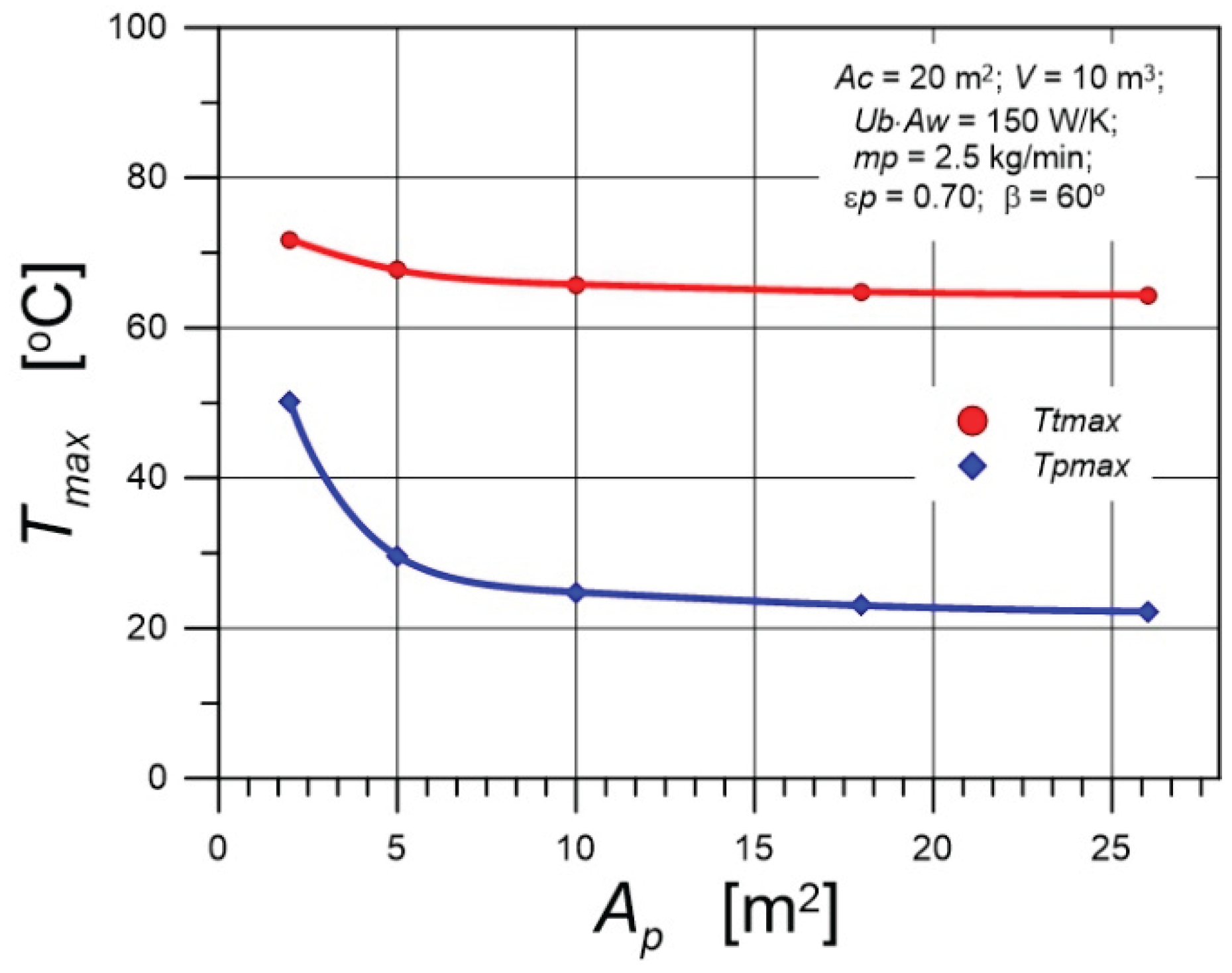
An important parameter affecting and is the pool surface area (Figure 19). The fixed value of determines based on the assumed pool depth of 1.35 m. For > 10 m2, maximum is approximately 21 °C, and maximum is about 61 °C. However, significant changes occur for small ; for example, for < 2 m², the maximum exceeds 50 °C.
6. Conclusions
This article presents a model of the process of heating a residential building and a pool with solar energy obtained by solar collectors and then stored in a heat storage tank. The analyses presented, based on the concept of solar utilizability, concerned the heating of a single-family house in a temperate climate. They demonstrated that removal of excess heat is a beneficial solution, especially when it can be used to heat water in a pool.
The main conclusions are as follows:
- (1)
- The method proposed by the authors combines the concept of solar utilizability with a functional approximation of physical and geometric quantities that undergo cyclical changes throughout the year. It generates smooth curves, disregarding short-term fluctuations in weather conditions relative to the average values. The developed numerical model enables quick and comprehensive analysis of the process and assessment of heat fluxes and temperatures occurring in the solar heating system for buildings and pools.
- (2)
- For the input data used in simulation calculations, the thermal effects of heating the pool are insufficient. In general, the water in pools is heated to 25-30°C. However, the purpose of this article was to examine the effect of using excess heat generated for space heating during the heating season; heating the water in the pool was only a result of this process. For the considered input data pool water temperature throughout the heating period was approximately 5-6 K higher than the air temperature, and the water temperature in the tank was relatively stable. The largest contribution to pool water heating comes from heat absorbed directly from solar radiation. The greatest heat losses in the pool are due to evaporative heat flux.
- (3)
- The impact of the solar collectors' area on the solar efficiency and solar fraction indicators was analyzed. Achieving values close to unity in temperate climates is quite difficult. It requires the use of large collector areas and large tank volumes. However, since buildings are always equipped with additional heat sources, it is advisable to forego high values in favour of increasing . This can be achieved by heating the water in the pool with excess heat from the solar installation. With increase, rises monotonically. The impact of is quite different for - the - curve has a maximum for small values of .
- (4)
- Climatic conditions have a strong influence on pool water temperature. A change in air humidity from 0.3 to 0.9 causes an increase in the maximum value of pool water temperature by 6 K. An increase in wind speed of 1.5 m/s can cause a reduction of 3 K in the maximum pool water temperature. Mass losses caused by water evaporation from pools are significant. For air at a temperature of 20 °C and relative humidity of 0.7, and water temperature of 23 °C, the difference in partial water vapor pressure above the water surface is 1170 Pa. Assuming a heat transfer coefficient (for u=0.5 m/s) of h = 7.6 W/(m2K), the evaporating water stream is equal to 0.22 kg/(m²∙h). Thus, approximately 0.09 m3 of water evaporates from a pool with an area of 18 m² per day.
- (5)
- Transferring excess heat from the storage tank does not reduce the potential heating capabilities of the space heating system. Therefore, this action is equivalent to improving the thermal performance of solar heating systems.
Author Contributions
Conceptualization, K.K. and S.P.; methodology, K.K.; software, K.K. and S.P.; validation, K.K.; formal analysis, K.K. and S.P.; investigation, K.K. and S.P.; resources, K.K. and S.P.; data curation, K.K. and S.P.; writing—original draft preparation, K.K. and S.P.; writing—review and editing, K.K. and S.P.; visualization, K.K. and S.P.; supervision, K.K. and S.P.; project administration, K.K. and S.P. All authors have read and agreed to the published version of the manuscript.
Funding
This research received no external funding.
Institutional Review Board Statement
Not applicable.
Informed Consent Statement
Not applicable.
Data Availability Statement
The data used in this study can be obtained from the corresponding author upon request.
Conflicts of Interest
The authors declare no conflicts of interest.
Nomenclature
| solar collectors' surface area, m2; | |
| pool surface area, m2; | |
| c | heat capacity, J/(kgK); |
| DDa | annual degree-days, K·day; |
| DDm | monthly degree-days, K·day; |
| evaporative heat flux, W/m2; | |
| collector heat removal factor; | |
| heat transfer coefficient, W/(m2K); | |
| daily radiation on the horizontal surface, J/m2; | |
| convective flux, W/m2; | |
| daily radiation on a tilted surface, J/m2; | |
| deep of the pool, m; | |
| daily radiation outside the atmosphere, J/m2; | |
| daily clearness index; | |
| long-wave radiation flux, W/m2; | |
| n | day of the year; |
| mass flow rate in the building circuit, kg/s; | |
| mass flow rate in the pool circuit, kg/s; | |
| mass of building, kg; | |
| daily heat accumulated in the walls of the building, J; | |
| daily heat from auxiliary source, J; | |
| daily heat required for space heating, J; | |
| daily tank heat losses, J; | |
| daily excess heat transferred to the pool, J; | |
| daily heat transferred to the building, J; | |
| daily useful heat, J; | |
| PVGIS | Photovoltaic Geographical Information System; |
| daily average beam radiation on the tilted surface, J/m2; | |
| air humidity; | |
| SC | solar collector; |
| solar efficiency defined by Eq.(19); | |
| solar fraction defined by Eq.(18); | |
| T | temperature, oC; |
| air temperature, oC; | |
| tank surroundings temperature, oC; | |
| inlet water temperature of the radiator in the room, oC; | |
| pool water temperature, K or oC; | |
| room temperature in the building, oC; | |
| sky temperature, K; | |
| water temperature in tank, oC; | |
| building walls temperature, oC; | |
| u | wind speed, m/s; |
| overall heat transfer coefficient of the whole building, W/(m2K); | |
| overall heat transfer coefficient of the tank, W/(m2K); | |
| volume of tank, m3; | |
| water volume in the pool, m3; | |
| time step ( = 1 day); | |
| daily variation of the water temperature in the tank, oC; | |
| internal energy change of the pool water, J; | |
| effective transmittance – absorptance product; | |
| β | collectors slope, rad or °; |
| ε | effectiveness of heat exchanger; |
| effectiveness of the pool heat exchanger; | |
| water density, kg/m3; | |
| diffuse reflectance; | |
| Stefan-Boltzmann constant, 5.67×10⁻⁸ W m⁻² K⁻⁴; | |
| summing from 1 to 365 days; | |
| daily utilizability; | |
| ψ | latitude, °; |
Appendix A. The Simultaneous Heat and Mass Transfer
The amount of heat lost per day as a result of evaporation of moisture from the water surface EV is determined based on the amount of evaporated water. The evaporative flux is determined by the mass transfer equation:
where and are respectively the water vapor concentrations on the water surface and in the surrounding air, is the mass transfer coefficient and is water's heat of vaporization.
According to Chilton-Colburn's analogy of heat and mass transfer [29], and are related by the following equation:
where is the specific heat of air, and is the Lewis number defined as the ratio of thermal diffusivity to mass diffusivity :
There is a relationship between the driving forces of evaporation expressed by concentrations and partial pressures:
where and are respectively the saturated vapor pressure at the water surface and partial vapor pressure in the atmospheric air, and is the total pressure. The saturated vapor pressure depends on temperature. This relationship is well described by Antoine's empirical equation [29], which for water is ([Pa], [℃]):
Combining the above relationships, we obtain:
where is a constant:
To determine the constant , numerical values of parameters should be used: molar masses of water and air = 0.018 kg/mol, = 0.029 kg/mol, = 2.48·106 J/kg, the diffusion coefficient of water in air = 22.5·10-6 m2/s, and the physical properties of air: = 1010 J/(kg·K) and = 19.4·10-6 m2/s [29]. For the air-water system, = 0.862 was determined. For a pressure = 1·105 Pa, = 0.0168 K/Pa was obtained.
References
- Sweet, M.L.; McLeskey, J.T. Numerical simulation of underground Seasonal Solar Thermal Energy Storage (SSTES) for a single family dwelling using TRNSYS. Sol. Energy 2012, 86, 289–300. [Google Scholar] [CrossRef]
- Soni, N.; Sharma, D.; Rahman, M.M.; Hanmaiahgari, P.R.; Reddy, V.M. Mathematical Modeling of Solar Energy based Thermal Energy Storage for House Heating in Winter. J. Energy Storage 2021, 34, 102203. [Google Scholar] [CrossRef]
- Redpath, D.; Colclough, S.; Griffiths, P.; Hewitt, N. Solar Thermal Energy Storage for the Typical European Dwelling; Available Resources, Storage Requirements and Demand. 2015, 1–9. [CrossRef]
- Clarke, J.; Colclough, S.; Griffiths, P.; McLeskey, J.T. A passive house with seasonal solar energy store: In situ data and numerical modelling. Int. J. Ambient Energy 2014, 35, 37–50. [Google Scholar] [CrossRef]
- Antoniadis, C.N.; Martinopoulos, G. Optimization of a building integrated solar thermal system with seasonal storage using TRNSYS. Renew. Energy 2019, 137, 56–66. [Google Scholar] [CrossRef]
- Villasmil, W.; Troxler, M.; Hendry, R.; Schuetz, P.; Worlitschek, J. Control strategies of solar heating systems coupled with seasonal thermal energy storage in self-sufficient buildings. J. Energy Storage 2021, 42. [Google Scholar] [CrossRef]
- Meister, C.; Beausoleil-Morrison, I. Experimental and modelled performance of a building-scale solar thermal system with seasonal storage water tank. Sol. Energy 2021, 222, 145–159. [Google Scholar] [CrossRef]
- Brites, G.J.; Garruço, M.; Fernandes, M.S.; Sá Pinto, D.M.; Gaspar, A.R. Seasonal storage for space heating using solar DHW surplus. Renew. Energy 2024, 231. [Google Scholar] [CrossRef]
- Kupiec, K.; Pater, S. On the possibility of achieving high solar fractions for space heating in temperate climates. Sol. Energy 2025, 300, 113789. [Google Scholar] [CrossRef]
- Kupiec, K.; Król, B. Optimal Collector Tilt Angle to Maximize Solar Fraction in Residential Heating Systems: A Numerical Study for Temperate Climates. Sustain. 2025, 17. [Google Scholar] [CrossRef]
- Lugo, S.; Morales, L.I.; Best, R.; Gómez, V.H.; García-Valladares, O. Numerical simulation and experimental validation of an outdoor-swimming-pool solar heating system in warm climates. Sol. Energy 2019, 189, 45–56. [Google Scholar] [CrossRef]
- Tagliafico, L.A.; Scarpa, F.; Tagliafico, G.; Valsuani, F. An approach to energy saving assessment of solar assisted heat pumps for swimming pool water heating. Energy Build. 2012, 55, 833–840. [Google Scholar] [CrossRef]
- Chow, T.T.; Bai, Y.; Fong, K.F.; Lin, Z. Analysis of a solar assisted heat pump system for indoor swimming pool water and space heating. Appl. Energy 2012, 100, 309–317. [Google Scholar] [CrossRef]
- Ilgaz, R.; Yumrutaş, R. Heating performance of swimming pool incorporated solar assisted heat pump and underground thermal energy storage tank: A case study. Int. J. Energy Res. 2022, 46, 1008–1031. [Google Scholar] [CrossRef]
- Li, Y.; Nord, N.; Huang, G.; Li, X. Swimming pool heating technology: A state-of-the-art review. Build. Simul. 2021, 14, 421–440. [Google Scholar] [CrossRef]
- Zhao, J.; Bilbao, J.I.; Spooner, E.D.; Sproul, A.B. Experimental study of a solar pool heating system under lower flow and low pump speed conditions. Renew. Energy 2018, 119, 320–335. [Google Scholar] [CrossRef]
- Li, Y.; Nord, N.; Yin, H.; Pan, G. Impact of heat loss from storage tank with phase change material on the performance of a solar-assisted heat pump system. Renew. Energy 2025, 241, 122208. [Google Scholar] [CrossRef]
- Li, Y.; Liang, J.; Chen, W.; Wu, Z.; Yin, H. Optimal design of a solar-assisted heat pump system with PCM tank for swimming pool utilization. Renew. Energy 2025, 240, 122272. [Google Scholar] [CrossRef]
- Starke, A.R.; Cardemil, J.M.; Colle, S. Multi-objective optimization of a solar-assisted heat pump for swimming pool heating using genetic algorithm. Appl. Therm. Eng. 2018, 142, 118–126. [Google Scholar] [CrossRef]
- Gonçalves, R.S.; Palmero-Marrero, A.I.; Oliveira, A.C. Analysis of swimming pool solar heating using the utilizability method. Energy Reports 2020, 6, 717–724. [Google Scholar] [CrossRef]
- Faisal Ahmed, S.; Khalid, M.; Vaka, M.; Walvekar, R.; Numan, A.; Khaliq Rasheed, A.; Mujawar Mubarak, N. Recent progress in solar water heaters and solar collectors: A comprehensive review. Therm. Sci. Eng. Prog. 2021, 25, 100981. [Google Scholar] [CrossRef]
- Olczak, P.; Matuszewska, D.; Zabagło, J. The comparison of solar energy gaining effectiveness between flat plate collectors and evacuated tube collectors with heat pipe: Case study. Energies 2020, 13. [Google Scholar] [CrossRef]
- Braun, J.E.; Klein, S.A.; Mitchell, J.W. Seasonal storage of energy in solar heating. Sol. Energy 1981, 26, 403–411. [Google Scholar] [CrossRef]
- Chiasson, A.D. Geothermal Heat Pump and Heat Engine Systems: Theory And Practice; John Wiley & Sons, Ltd., 2016; ISBN 9781118961940.
- Goswami, D.Y. Principles of Solar Engineering; CRC Press, Taylor & Francis Group: Boca Raton, 2022; ISBN 9781003244387. [Google Scholar]
- Kalogirou, S.A. Solar Energy Engineering: Processes and Systems; Elsevier Inc, 2009; ISBN 9780123745019.
- European Commission, Photovoltaic Geographical Information System. Available online: https://re.jrc.ec.europa.eu/pvg_tools/en/ (accessed on 22 August 2025).
- Duffie, J.A.; Beckman, W.A. Solar Engineering of Thermal Processes; Fourth.; John Wiley & Sons, 2013; ISBN 978-0-470-87366-3.
- Perry, S.; Perry, R.H.; Green, D.W.; Maloney, J.O. Perry’s chemical engineers’ handbook; 2000; Vol. 38; ISBN 0070498415.
Figure 1.
Solar system diagram.
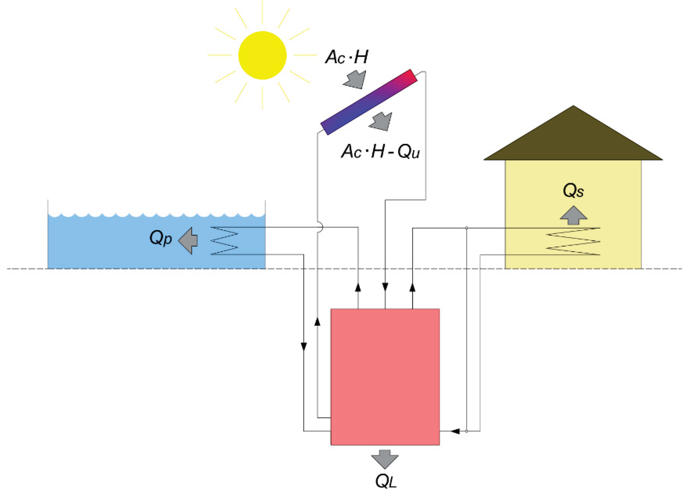
Figure 2.
Sankey diagram for solar heating system.
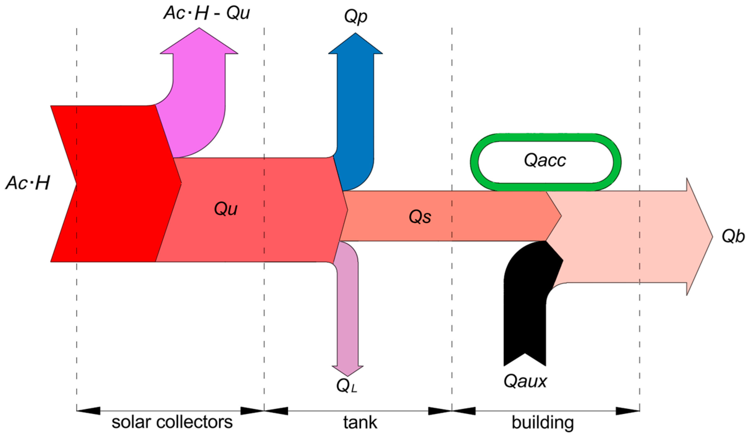
Figure 3.
Explanation of the heating water flow switching.
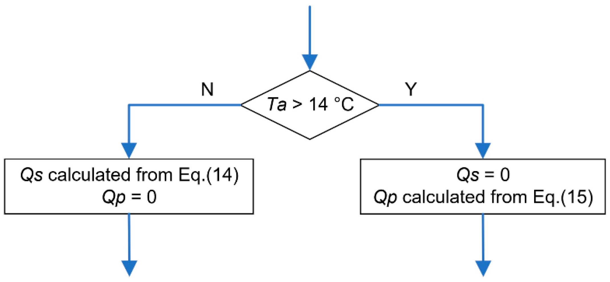
Figure 4.
Heat fluxes during pool heating.
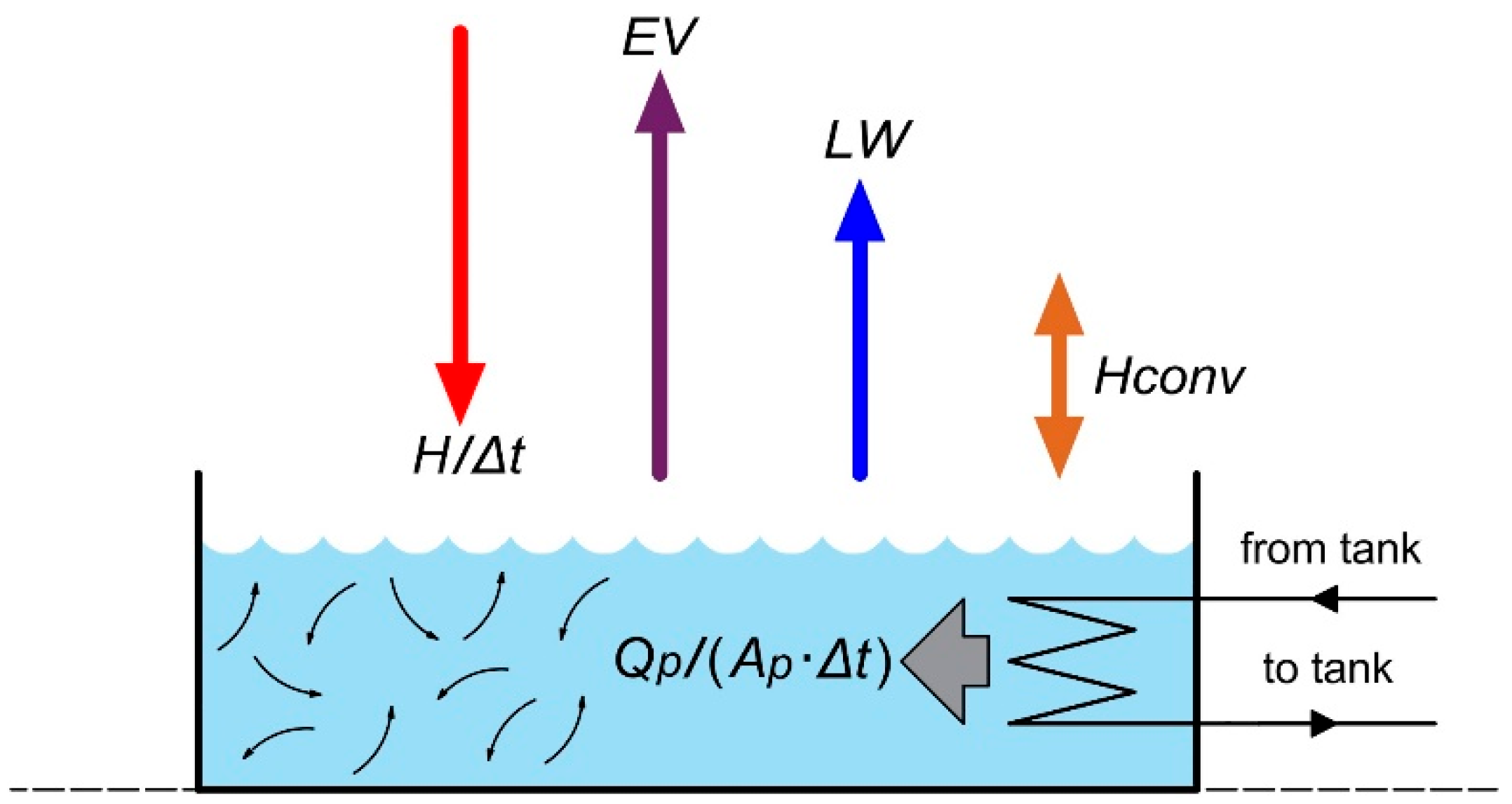
Figure 5.
Approximation of the temporal temperature course.
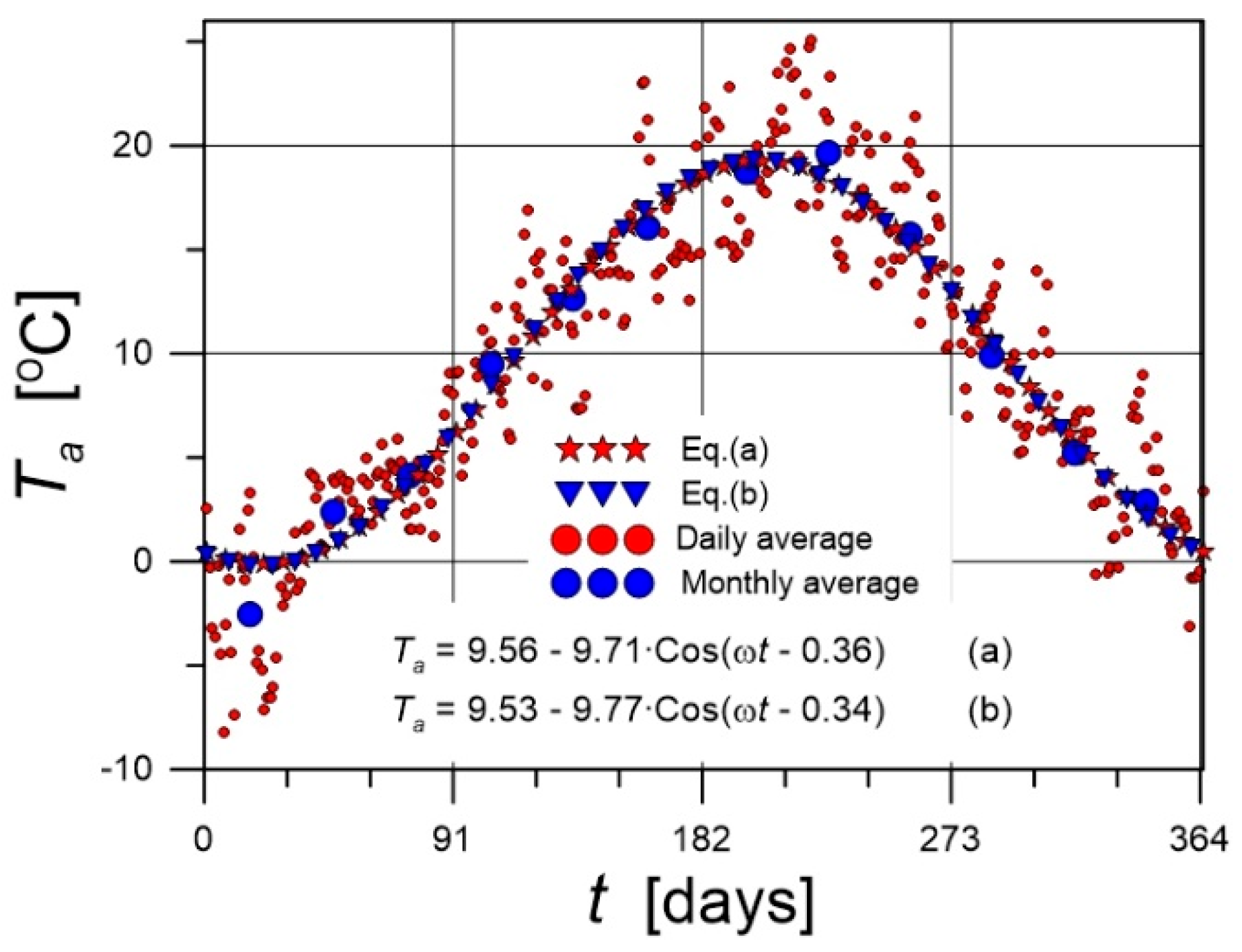
Figure 6.
Approximation of daily solar radiation on a horizontal surface.
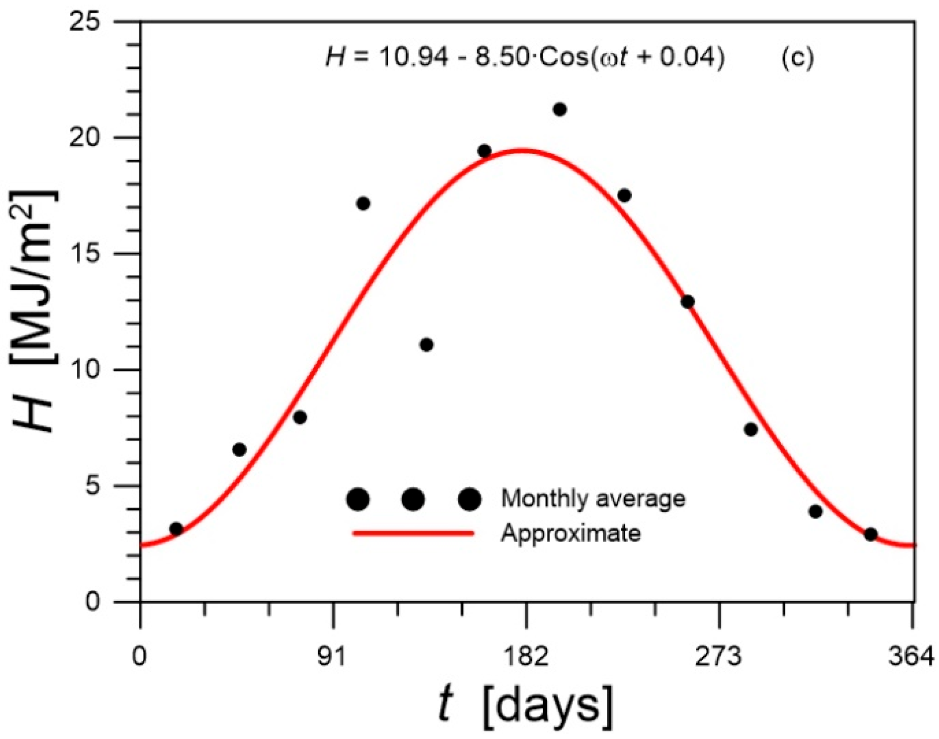
Figure 7.
The influence of on .
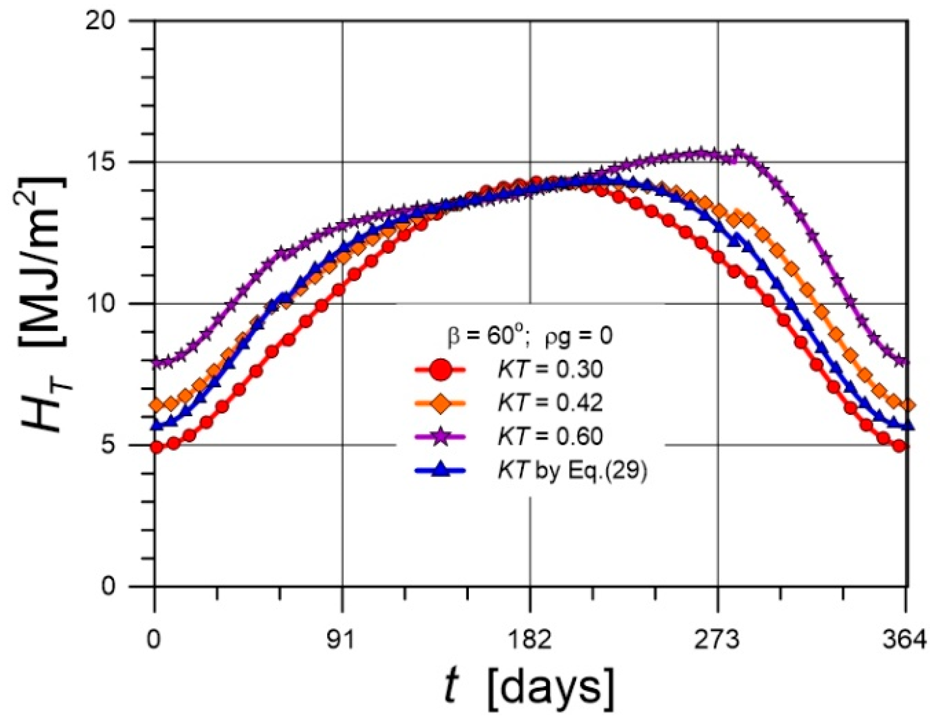
Figure 8.
The influence of β and on .
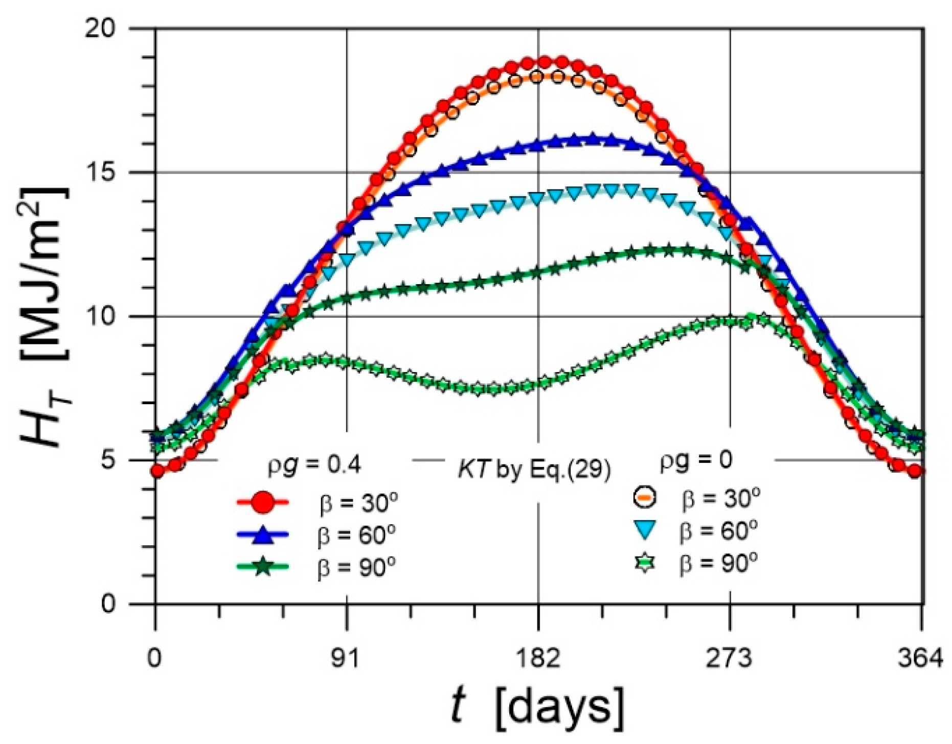
Figure 9.
Time courses of solar radiation in various conditions.
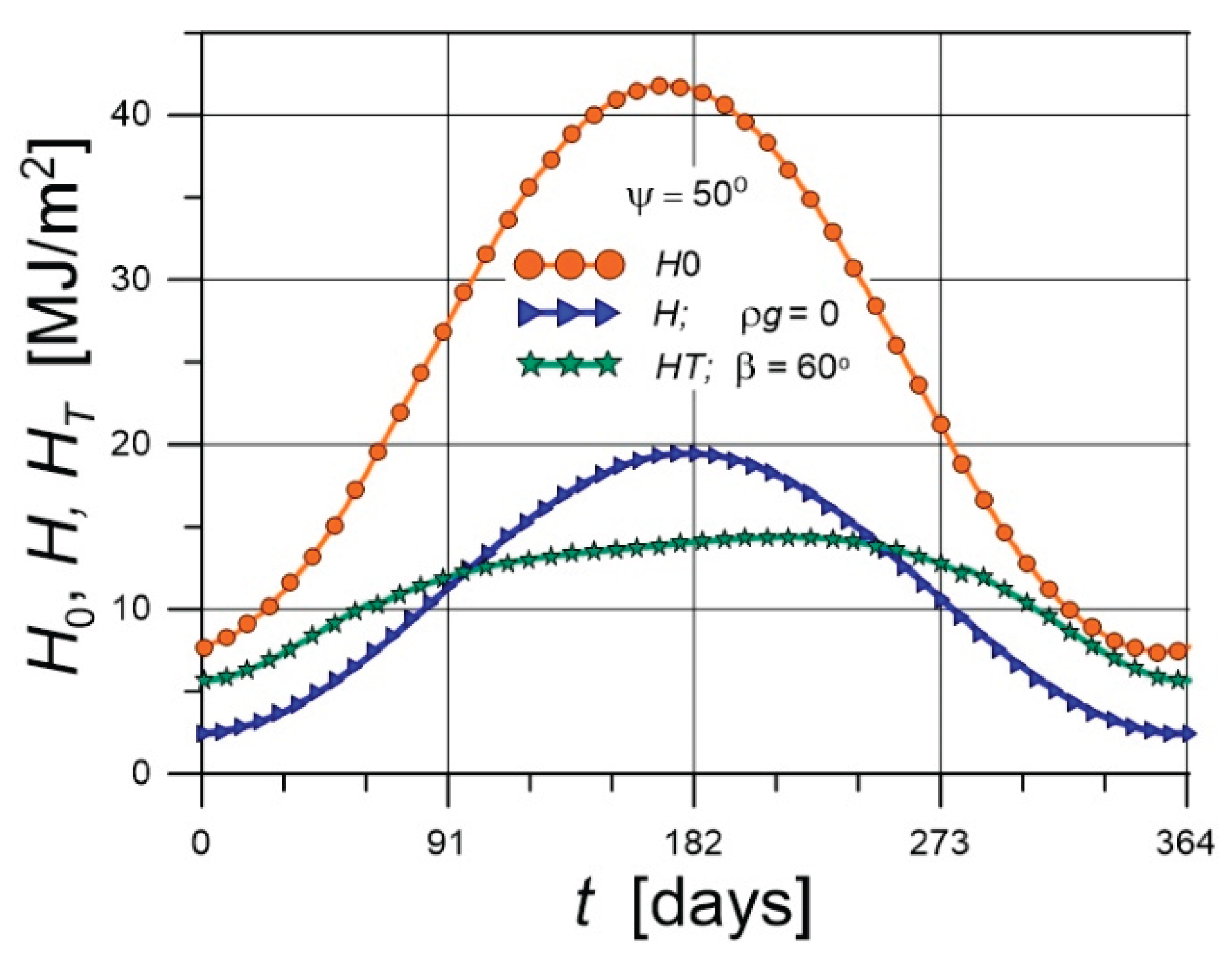
Figure 10.
Daily heats in a solar system.
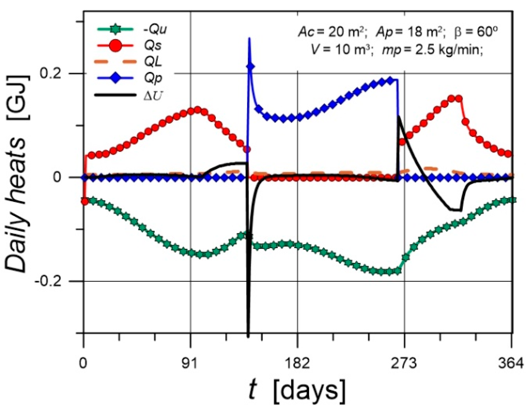
Figure 11.
Time courses of and .
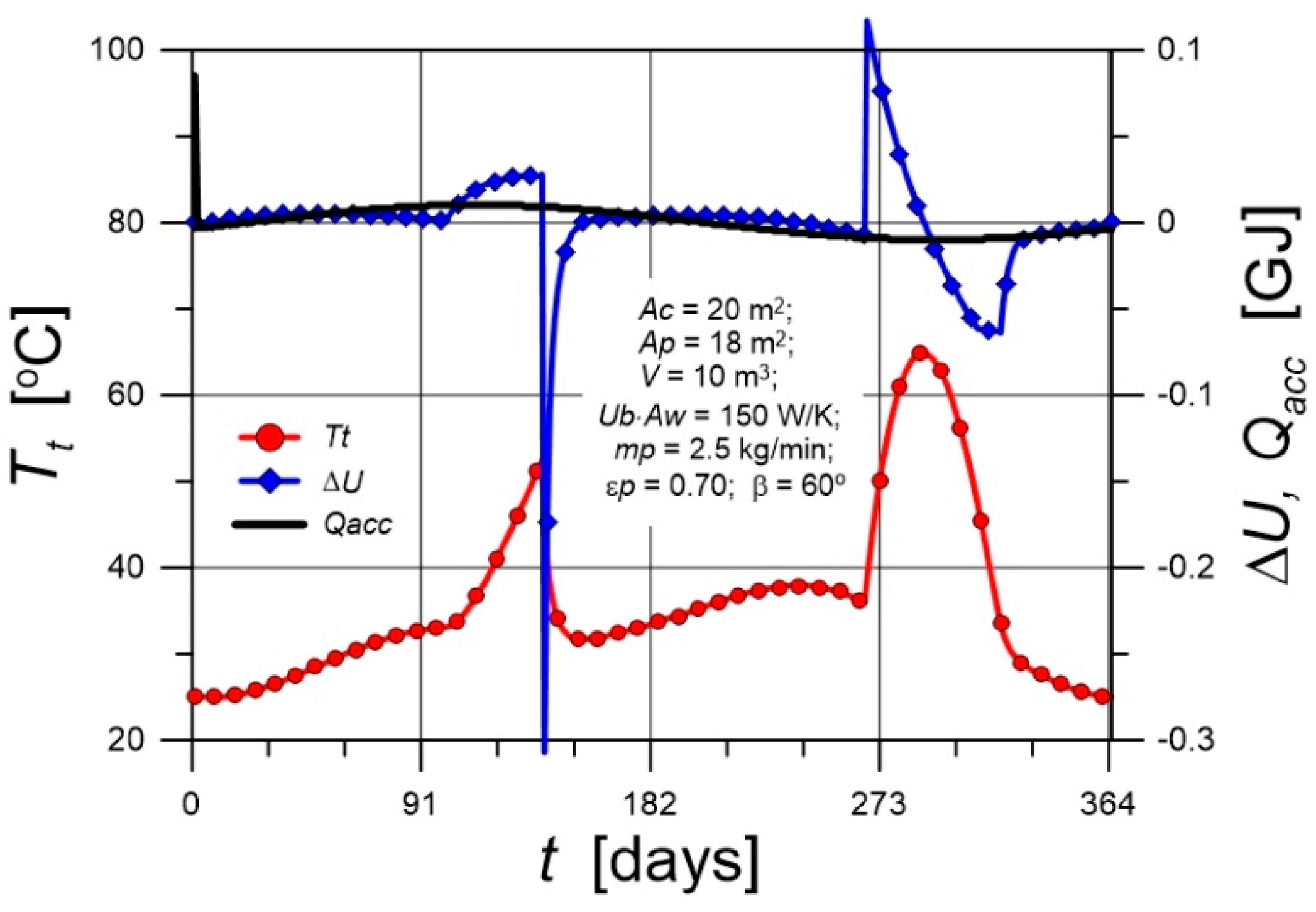
Figure 12.
Temperature coursers in solar system.
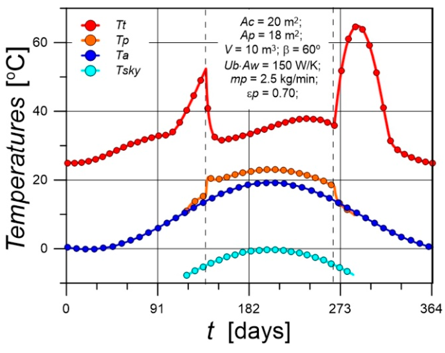
Figure 13.
Heat rates in solar system.
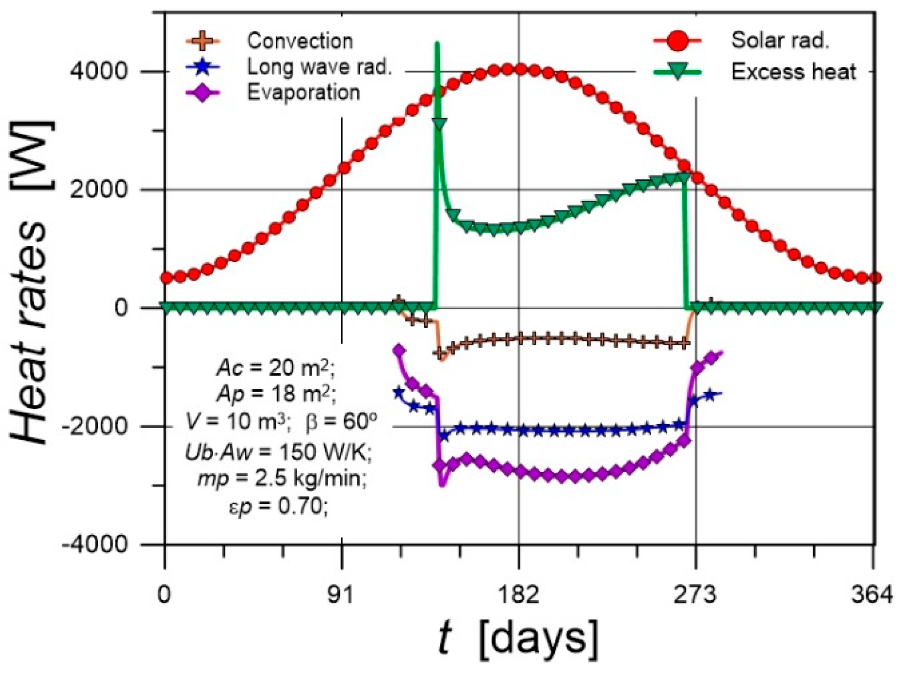
Figure 14.
Time courses of at different values.
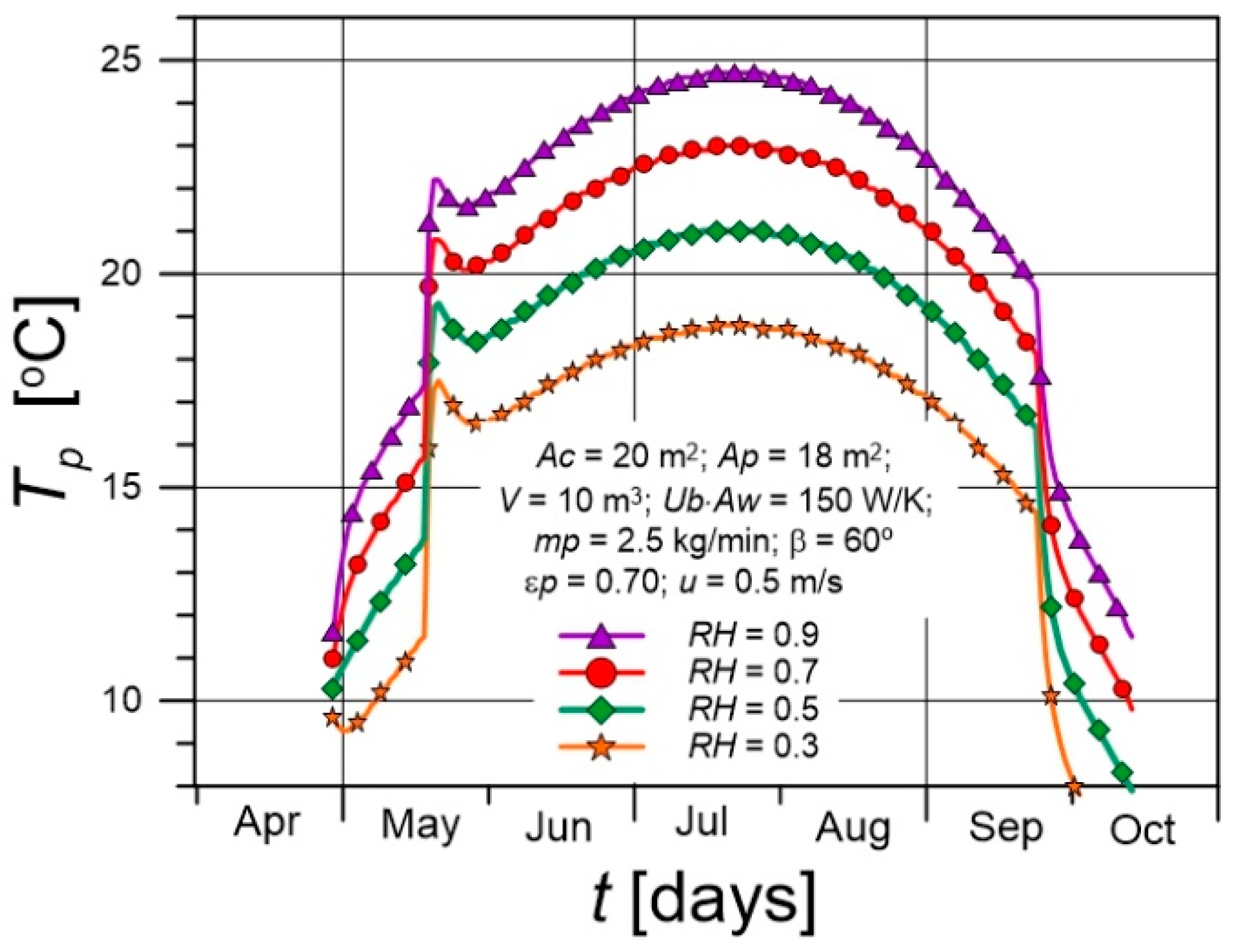
Figure 15.
Time courses of at different wind speed values.
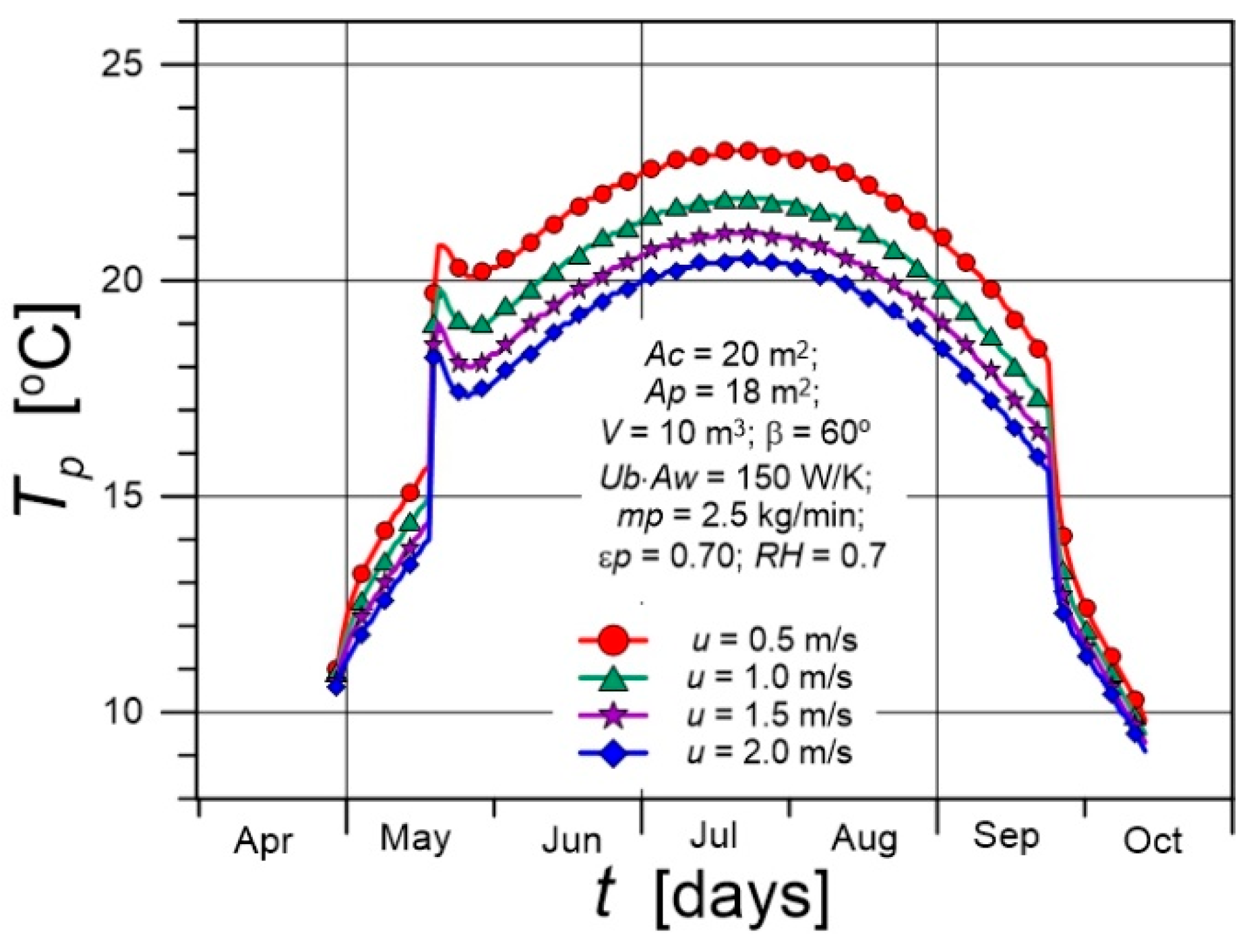
Figure 16.
Influence of on , , , and the maximum .
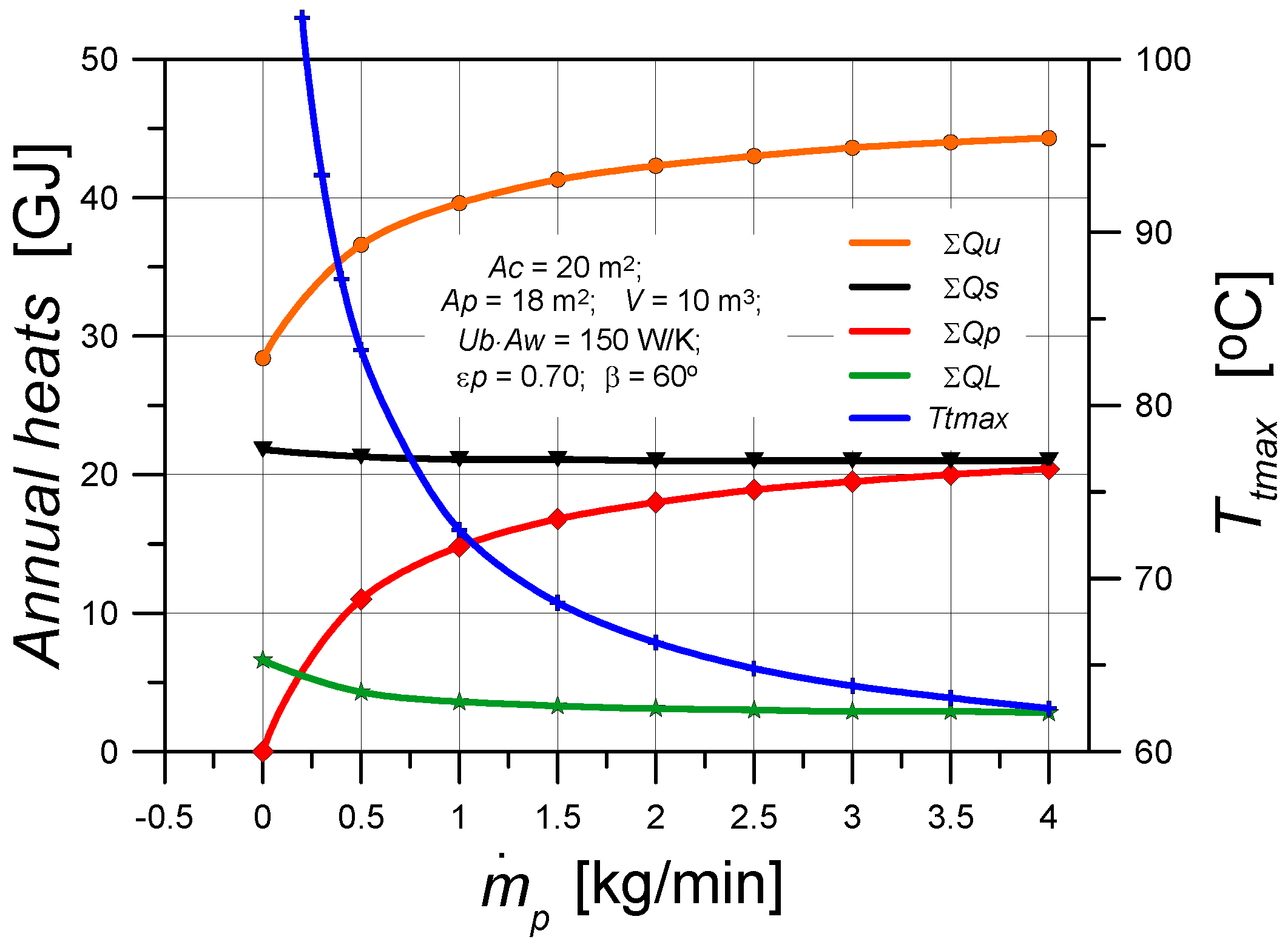
Figure 17.
Influence of on and .
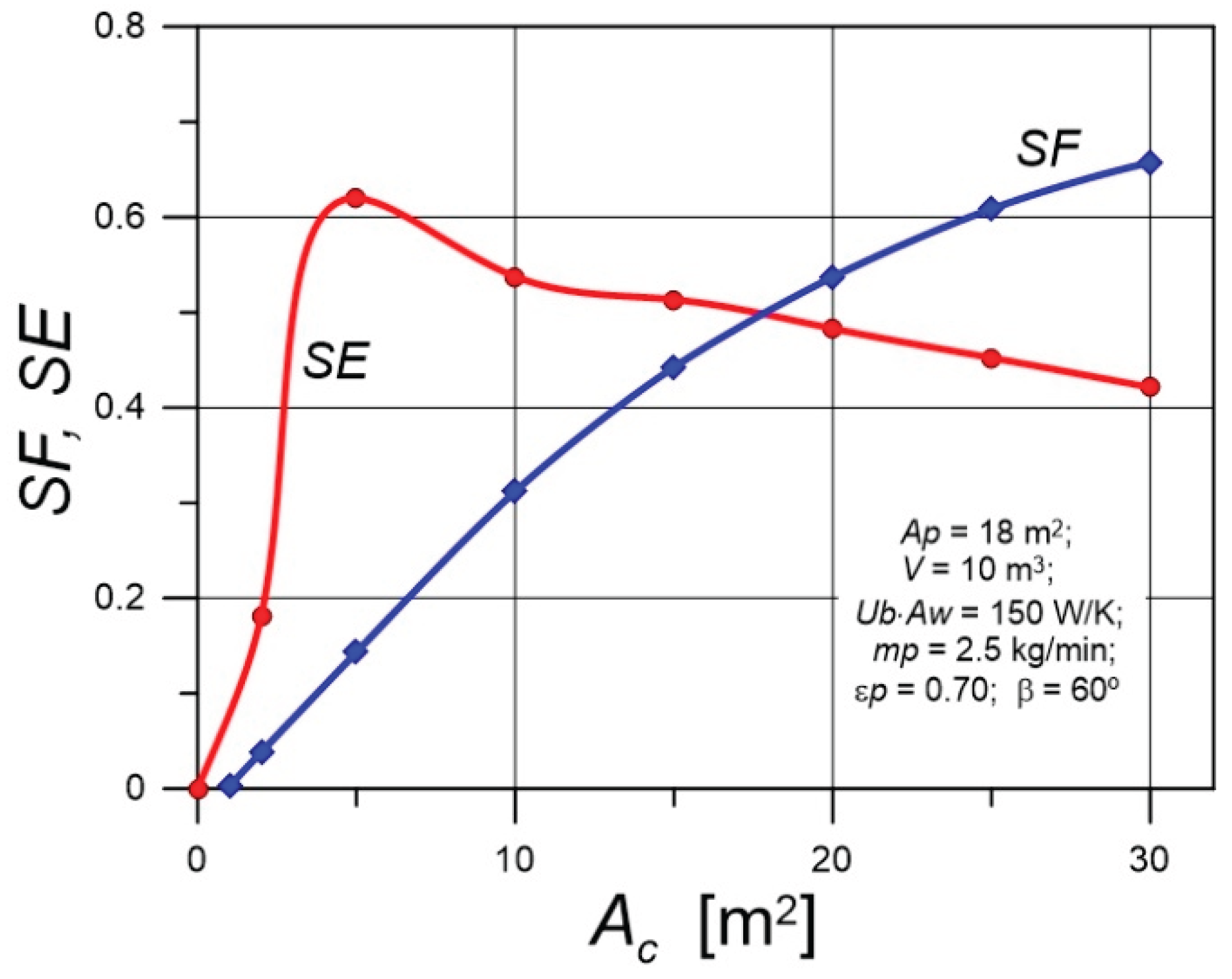
Figure 18.
Influence of on , , , and the maximum .
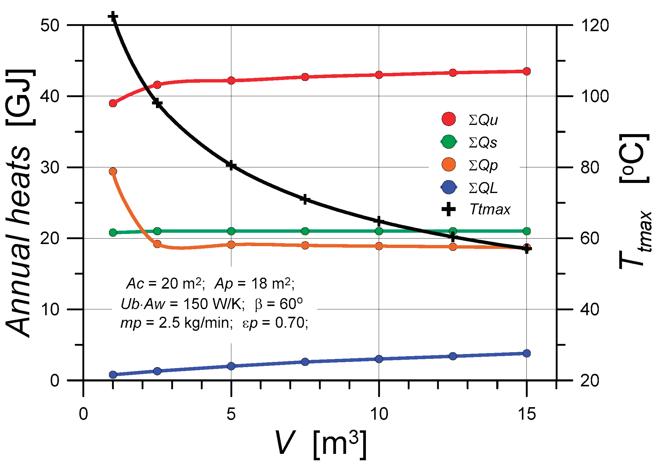
Figure 19.
Influence of on the maximum and .

Disclaimer/Publisher’s Note: The statements, opinions and data contained in all publications are solely those of the individual author(s) and contributor(s) and not of MDPI and/or the editor(s). MDPI and/or the editor(s) disclaim responsibility for any injury to people or property resulting from any ideas, methods, instructions or products referred to in the content. |
© 2025 by the authors. Licensee MDPI, Basel, Switzerland. This article is an open access article distributed under the terms and conditions of the Creative Commons Attribution (CC BY) license (http://creativecommons.org/licenses/by/4.0/).
Copyright: This open access article is published under a Creative Commons CC BY 4.0 license, which permit the free download, distribution, and reuse, provided that the author and preprint are cited in any reuse.


