Submitted:
04 September 2025
Posted:
08 September 2025
You are already at the latest version
Abstract
We study the negative discrete moments of the derivative of the Riemann zeta function at its nontrivial zeros, in connection with the Hughes--Keating--O’Connell conjecture. Building on the works of Gonek, Milinovich--Ng, Kirila, and the recent breakthrough of Bui--Florea--Milinovich, we introduce a new \emph{entropy--sieve method} (ESM). This framework combines short Dirichlet-polynomial approximations with entropy-based moment generating function bounds and a small-gap sieve, thereby controlling all appearances of $\zeta'(\rho)$ without assuming simplicity of zeros.Assuming the Riemann Hypothesis together with standard pair-correlation conjectures and a strengthened discrete moment hypothesis, we prove the quantified conditional bound \[ J_{-1}(T) \;=\; \sum_{0<\gamma\leq T} \frac{1}{|\zeta'(\tfrac12+i\gamma)|^{2}} \;\le\; C(\varepsilon)\, T (\log T)^{\varepsilon}, \qquad \text{for every fixed $\varepsilon>0$}, \] with an explicit dependence of the implicit constant on $\varepsilon$. This matches, up to logarithmic factors, the conjectured order $J_{-1}(T)\asymp T$ and improves on all previous conditional results.The analysis introduces several innovations: (i) a full cumulant control lemma for Dirichlet polynomials; (ii) explicit, non-circular parameter selection for approximation lengths and moments; and (iii) an entropy--sieve hybrid decay lemma that quantifies large-deviation probabilities for $\zeta'(\rho)$. Beyond the negative moment problem, the entropy--sieve framework illustrates the strength of entropy techniques in analytic number theory and points toward applications to $L$-functions and random matrix models.
Keywords:
Riemann zeta function
; Dirichlet polynomials
; entropy bounds
; cumulant factorization
; negative moments
For the reader’s convenience, we summarize the main notation that will be used consistently throughout the paper. Our framework combines classical Dirichlet-polynomial approximations with entropy-based tools, so the table below records both standard analytic objects and the new entropy-related quantities.

Table 1.
Notation for general quantities, Dirichlet-polynomial approximations, moment generating functions, and entropy framework.
Table 1.
Notation for general quantities, Dirichlet-polynomial approximations, moment generating functions, and entropy framework.
| General Notation | |
|---|---|
| T | Height parameter for critical zeros of . Zeros with . |
| Number of zeros with . | |
| Nontrivial zero of , written . | |
| Imaginary ordinate of a zero. | |
| Exceptional set where Dirichlet-polynomial approximation fails (Lemma 8). | |
| Exceptional set of zeros lying in low-entropy blocks (Lemma 4). | |
| Set of “good” zeros (outside all exceptional sets). | |
| Set of simple zeros . | |
| Dirichlet Polynomial Approximation | |
| X | Dirichlet polynomial length . |
| A | Truncation exponent. |
| Approximant . | |
| Dirichlet polynomial coefficients. | |
| Error term in approximation of . | |
| Variance of : (Lemma 2). | |
| Y | Auxiliary parameter . |
| Moment Generating Function & Tail Estimates | |
| Moment generating function: . | |
| r-th cumulant of . | |
| Raw r-th moment of . | |
| t | Auxiliary parameter, . |
| Admissible t: (Proposition 1). | |
| Tail count: . | |
| V | Threshold parameter in tail bounds. |
| Constant governing MGF tail decay. | |
| Entropy Framework (Section 3) | |
| Local window of zeros near . | |
| Value entropy (Definition 1). | |
| Gap entropy of zero spacings (Definition 2). | |
| Entropy threshold used to classify blocks. | |
| Bin widths for histograms. | |
| Histogram bins for values and gaps. | |
| Empirical frequency of value bin . | |
| Empirical frequency of gap bin . | |
| Shannon entropy of values. | |
| Shannon entropy of normalized gaps. | |
Table 2.
Notation for discrete moments, sieve parameters, and hypotheses.
| Moments and Sieve | |
|---|---|
| Discrete -moment: . | |
| Same sum restricted to simple zeros. | |
| Small-gap cutoff (Definition 3). | |
| Exponent in . | |
| Set of zeros with normalized gaps . | |
| Block of m consecutive zeros centered at . | |
| m | Entropy block length (see Section 3). |
| Pair-Correlation Hypothesis (see Section 3). | |
| Discrete Moment Control hypothesis. | |
| Small-Gap Estimate hypothesis. | |
| Positive constants from Gaussian, entropy, and sieve bounds. | |
Table 3.
Notation for discrete moments, sieve parameters, and hypotheses.
| Moments and Sieve | |
|---|---|
| Discrete moment: . | |
| Same sum restricted to simple zeros. | |
| Small-gap cutoff: . | |
| Exponent in small-gap threshold. | |
| Set of zeros with normalized gaps . | |
| Block of m consecutive zeros centered at . | |
| m | Entropy block length. |
| Pair-Correlation Hypothesis. | |
| Discrete Moment Control hypothesis. | |
| Small-Gap Estimate hypothesis. | |
| Positive constants in Gaussian/entropy/sieve bounds. | |
1. Introduction
Let denote the Riemann zeta function and its nontrivial zeros. The size of the derivative at these zeros plays a central role in analytic number theory, with deep links to the distribution of zeros, random matrix theory, and the behavior of moments of L-functions. For , we define the discrete moment
where the sum runs over all nontrivial zeros of , counted with multiplicity. For this sum is finite only if every zero is simple, since a multiple zero would satisfy and force . Thus, understanding upper bounds for in the negative range not only addresses deep conjectures but also has direct implications for the simplicity of zeros.
1.1. Motivation and Conjectures
The asymptotic behavior of has been studied extensively. Based on random matrix heuristics, Hughes, Keating, and O’Connell [1][Conj. 1.7, p. 5] conjectured that for ,
where is the Barnes G-function and is an explicit arithmetic factor. In particular, for , conjecture (1) predicts
so the negative second moment should be of the same order as the number of zeros up to height T.
1.2. State of the Art
For positive moments (), major progress has been achieved:
- Gonek [2][p. 35] initiated the study of discrete moments of , deriving asymptotic formulas for under the Riemann Hypothesis (RH).
- Hejhal [3][Sec. 3] analyzed the distribution of and showed that it is approximately Gaussian with variance , providing a probabilistic model for small and large values of .
- Kirila [4][Thm. 1.1] obtained sharp upper bounds for positive moments by adapting Harper’s probabilistic Dirichlet-polynomial method:where is the number of zeros up to height T.
- Harper’s framework [7] introduced entropy-based large deviation bounds in multiplicative chaos models, tools later adapted to the zeta setting.
These results align with the Hughes–Keating–O’Connell conjecture for .
For negative moments (), progress is much more limited:
- Gonek [2][p. 36] obtained conditional lower bounds for but no general upper bounds.
- Milinovich and Ng [5] refined such lower bounds by relating to zero spacings.
- Most recently, Bui, Florea, and Milinovich [6] derived conditional upper bounds for negative moments over a large subfamily of zeros, excluding a sparse exceptional set where may be abnormally small. A complete bound for all zeros, however, remained out of reach.
1.3. Challenges for Negative Moments
The central difficulty in bounding with lies in controlling rare zeros where is exceptionally small. Since
the main contribution arises from these rare events. Hejhal’s Gaussian model [3] predicts that such events are exponentially rare, but turning this heuristic into rigorous uniform estimates requires two delicate ingredients:
1.4. Our Approach and Contributions
In this paper we introduce a hybrid analytic–probabilistic framework, the entropy–sieve method (ESM), which combines these two ideas systematically. Our contributions are as follows:
- Sieve for exceptional zeros: Following the philosophy of Bui–Florea–Milinovich [6], we apply a small-gap sieve to remove the remaining exceptional zeros. Our systematic parameter optimization clarifies how can be tuned to make all exceptional sets negligible.
-
Quantified negative moment bound: Under RH, pair-correlation hypotheses, and a strengthened discrete moment conjecture, we proveThe here is fully quantified, with explicit dependence of the implicit constant on parameter choices. This matches the HKO prediction up to logarithmic factors and sharpens all previous conditional results.
1.5. Organization
The remainder of the paper is structured as follows. Section 2 reviews prior results on positive and negative moments, emphasizing the conjectural framework of Hughes–Keating–O’Connell. Section 3 introduces the entropy–sieve method, combining Dirichlet-polynomial approximations with entropy regularity to yield robust Gaussian tail bounds. Section 6 develops the sieve-theoretic component, excluding low-entropy or small-gap exceptional sets. Finally, Section 7.9 combines these tools to prove the conditional upper bounds for in the range , with the quantified case as the centerpiece.
Main Results
- Entropy–Sieve Framework. We develop a new analytic–probabilistic method that combines entropy-decrement techniques with small-gap sieve bounds to control exceptional sets of zeros. This framework provides a unified approach to bounding negative moments of and clarifies the role of local entropy in the distribution of Dirichlet polynomial approximations.
- Quantified Conditional Bound for Negative Moments. Assuming the Riemann Hypothesis together with standard pair-correlation conjectures and a strengthened discrete moment hypothesis, we establish the boundvalid for every fixed , with an explicit dependence of the implicit constant on . This matches, up to logarithmic factors, the conjectured order predicted by Hughes–Keating–O’Connell, and improves on all previous conditional results by making the –dependence transparent.
- Entropy–Sieve Hybrid Decay (Lemma 8). We prove a uniform Gaussian tail bound for the frequency of zeros with exceptionally small derivative, valid up to deviations . The bound combines (i) full cumulant/MGF control for Dirichlet polynomials, (ii) a sieve for small gaps, and (iii) explicit exceptional set bounds. This lemma underpins the negative moment estimates.
- Simplicity of Zeros (Proposition 3). We avoid circularity by working with truncated reciprocals throughout. Under a strengthened pair-correlation hypothesis (PCH*), we deduce that the number of multiple zeros up to height T is for some . In particular, almost all zeros are simple under (PCH*).
- Joint MGF Bounds (Proposition 4). The mixed moment generating function of Dirichlet polynomial approximants admits a uniform Gaussian bound with covariance matrix , with cubic error terms of order .
- Parameter Bookkeeping. A compact parameter table records the definitions and admissible ranges of , clarifying the logical order of choices and eliminating ambiguity in the proofs.
- Numerical and Structural Evidence. The theoretical results are consistent with Odlyzko’s numerical data on zeros and with new computations. The entropy–sieve method is robust and suggests further applications to negative moments of L-functions and to analogues in random matrix theory.
2. Background
The discrete moments of the derivative of the Riemann zeta function at its nontrivial zeros,
are central objects in analytic number theory. They provide insight into the distribution of , the spacing of the nontrivial zeros of , and the connections between the zeta function and random matrix theory. Understanding the asymptotic growth of has been the subject of extensive research over the past decades and is closely connected with one of the most refined conjectures in this area: the Hughes–Keating–O’Connell conjecture.
2.1. The Hughes–Keating–O’Connell Conjecture
Motivated by random matrix theory and probabilistic models, Hughes, Keating, and O’Connell proposed an explicit formula for in the regime . Their conjecture predicts that
where denotes the Barnes G-function and is an explicit arithmetic factor arising from the Euler product.
This conjecture is supported by strong heuristics derived from the characteristic polynomials of random unitary matrices. In these models, behaves approximately like a Gaussian random variable, and formula (2) reflects the matching asymptotics between the number-theoretic and random-matrix frameworks. A striking consequence appears when setting , where the conjecture predicts
Thus, the negative second moment is conjectured to be of the same order as the number of zeros up to height T.
2.2. Positive Moments
The case of positive moments, , is relatively well understood and has seen substantial progress over the last four decades. Gonek [2][Thm. 1, p. 35] pioneered the study of discrete moments of , proving under the Riemann Hypothesis that for ,
This result agrees with the prediction of (2) when and represented one of the earliest confirmations of the conjecture in a special case.
Hejhal [3][Sec. 3, Thm. 3.1, pp. 343–370] advanced the probabilistic understanding of by studying the distribution of . He showed that, heuristically, behaves approximately like a Gaussian random variable with variance . This probabilistic model suggested that extremely large or small values of are exponentially rare and laid the conceptual foundation for later entropy-based methods.
A major breakthrough came from Harper [7][Thm. 2.1, pp. 5–20], who developed sharp techniques for bounding high moments of Dirichlet polynomials using ideas from multiplicative chaos theory. His method is based on entropy principles and Gaussian approximations, providing nearly optimal estimates for the moments of random multiplicative functions. Building on Harper’s framework, Kirila [4][Thm. 1.1, pp. 2–4] adapted these ideas to the discrete setting of the zeta zeros and obtained sharp conditional upper bounds for positive moments:
where denotes the number of zeros up to height T. These results are fully consistent with the random matrix predictions of the Hughes–Keating–O’Connell conjecture, providing strong evidence in favor of (2) for .
2.3. Negative Moments
In stark contrast to the positive regime, the behavior of for negative k remains largely mysterious. The primary challenge stems from the fact that negative moments are dominated by the contribution of zeros where is extremely small. Controlling this contribution requires strong bounds on the lower tail of , a problem that has resisted classical techniques.
Early work by Gonek [2][Thm. 2, p. 36] established conditional lower bounds for negative moments but provided no nontrivial upper bounds. Later, Milinovich and Ng [5][Prop. 4.1, pp. 642–644] refined these lower bounds by relating to the spacing between consecutive zeros, but even these methods do not yield control over the full sum.
A significant development came from Bui, Florea, and Milinovich [6][Thm. 1.3, pp. 3–6], who obtained the first partial progress toward bounding negative moments. By excluding a sparse exceptional set of zeros where is abnormally small, they proved conditional upper bounds for over a large subfamily of zeros. However, their results stop short of proving the full conjectured bound for or other negative moments over all zeros.
These contributions underline the difficulty of the negative moment problem: without precise control over extremely small values of , unconditional upper bounds remain out of reach. This motivates our entropy-sieve framework, designed to isolate and neutralize such exceptional contributions.
Hypotheses Used in This Paper
Our main results are conditional on several standard conjectural inputs. For clarity we record them here.
- (RH) Riemann Hypothesis. All nontrivial zeros of the Riemann zeta function lie on the critical line .
- (PCH) Pair–Correlation Hypothesis. For any fixed real u, one hasuniformly for for some fixed . Equivalently, Montgomery’s pair–correlation formula holds in this quantitative form for the frequency ranges needed in our Dirichlet–polynomial expansions.
-
(DMC) Discrete Moment Control. For any fixed and for Dirichlet polynomialswe haveIn particular, the moment generating function of short Dirichlet polynomials is well approximated by a Gaussian with variance , uniformly for .
- (SGE) Small-Gap Estimate. The number of pairs of consecutive zeros of with gap at most is , uniformly for and any fixed . This matches Montgomery’s pair–correlation predictions and is used in Section 7 to control large deviations of .
All later results should be read as conditional on (RH), (PCH), (DMC), and (SGE).
2.4. Summary
To summarize, positive moments of are now well understood, thanks to the interplay between Harper’s entropy-based techniques, Kirila’s discrete adaptations, and random matrix predictions. For negative moments, however, the lack of control over zeros with exceptionally small remains the key obstacle. Overcoming this barrier is essential for advancing toward a full resolution of the Hughes–Keating–O’Connell conjecture, particularly in the critical regime .
3. Entropy-Based Approximation and Gaussian Large-Deviation Bounds
Assumption Framework
Throughout this section we assume the Riemann Hypothesis (RH). For technical steps where denominators involving arise, we restrict initially to the set of simple zeros
and define discrete averages over in place of all zeros. This avoids divergences in moment calculations involving negative powers. No generality is lost, since has the same density as the full zero set under standard pair-correlation heuristics (cf. [17,28,29]).
In Section 3, we show that our joint MGF and block entropy bounds imply that the presence of multiple zeros in a positive-density set of ordinates is incompatible with the Gaussian limit law. In particular, Theorem 1 below establishes that, under RH and the verified block large-deviation estimates, all but zeros up to height T must in fact be simple. Thus the initial restriction to is later justified a posteriori.
3.1. Notation and Choice of Parameters
Fix large parameters (to be chosen later in terms of any desired power savings). For T large define
Both X and Y grow with T, with X a fixed power of and Y super-polynomial in but sub-polynomial in T. We shall construct a short Dirichlet polynomial of length X to approximate for most zeros .
For a generic Dirichlet polynomial
we define its variance
In our application the coefficients will be explicit (coming from a truncated Euler product or approximate functional equation for ), and we will have
uniformly for our range of parameters.
3.2. Dirichlet-Polynomial Approximation for
Choice of the Truncation Length X
Throughout this section we fix
with chosen large depending on the error exponents in subsequent lemmas. This polylogarithmic choice ensures that the Dirichlet polynomial approximation (Lemma 1) has a negligible error term, that the moment generating function bounds (Proposition 1) remain uniform for , and that block cumulant factorization (Lemma 5) can be applied without enlarging off-diagonal terms. We emphasize that with small fixed may also be treated with refinements of our arguments, but to avoid technical complications we restrict to the polylogarithmic case.
Hypotheses, Coefficients, and Quantitative Bounds
For clarity we record the precise setup that will be used throughout this section.
- Hypothesis. We assume the Riemann Hypothesis (RH). All multiple zeros are placed into the exceptional set .
- Truncation length. We fixwith A chosen large depending on the desired decay of the remainder (see Lemma 1).
- Coefficients. Let be a fixed smooth cutoff with for . Defineso is supported on prime powers and is explicit and computable.
- Dirichlet polynomial. For each zero we define
- Remainder and exceptional set. We setand define an exceptional setwhere is arbitrary.
- Quantitative bounds. For every there exists such thatand
These constants are uniform in T, and the implied constants depend only on the cutoff w and the chosen parameters . This hypothesis package is exactly what Lemma 1 will establish.
3.3. Choice of Dirichlet Polynomial Length and Variance Normalization
In earlier drafts of this work (and in some related literature), the Dirichlet polynomial approximating was taken of length , which yields a variance . In the present paper we adopt a different choice, namely
with A fixed and large. This modification has several consequences.
-
Variance scale. For coefficients with , the variance of the associated Dirichlet polynomial isThus throughout the paper, whenever we refer to the variance parameter , it should be understood thatnot .
-
Range of admissible t. Since the cumulant method requires , we now work withAll later appearances of the “admissible t–range” should be interpreted accordingly. In particular, the entry for in Table should read .
- Range of V. In tail estimates (e.g. Lemma 7.2), the permissible rangeshould be read with . Thus the Gaussian-type decay controls tails up to scale .
This normalization explains why some statements (drafted with ) refer to rather than . From this point onward we uniformly adopt the -length model, so that all variance and admissible-t bounds are understood in the scale.
4. Derivation of the Coefficients from a Smoothed Explicit Formula
In this section we derive explicitly the prime-power coefficients appearing in the short Dirichlet polynomial approximants
and we record the decomposition of the remainder arising from the contour shift. Our derivation follows the standard smoothed explicit-formula method; see Davenport [8][Ch. 12 and Ch. 21] for the classical treatment of the explicit formula and truncation estimates, and Hejhal [3][pp. 343–370] for the adaptation to .
1. Smoothed Representation of and Differentiation
For we have the Dirichlet series expansion
where denotes the small analytic correction arising from the pole at . Insert the smooth cutoff
with w compactly supported, on , so that for and for . Define the truncated series
Differentiating formally gives
Thus the coefficients are supported on prime powers .
2. Contour Integral and Explicit Formula
To access , one introduces a smooth Mellin kernel V with compact support and considers the integral
where is a zero and . Unfolding the integral yields
with a small tail term . Shifting the contour across and collecting residues gives the explicit identity (valid for simple zeros, see Hejhal [3][pp. 343–370]):
3. Coefficients and Remainder Terms
The coefficients are explicitly
where are explicit boundary correction weights. The remainder terms in (8) are:
- : the contribution from ; for every ,see [8][Ch. 21].
- : boundary integrals from the contour shift; these satisfy for each ,
4. Quantitative Consequences
Bibliographic Note
The derivation above is the standard explicit-formula method with smoothing: the integral representation, contour shift, and kernel construction are detailed in Hejhal [3][pp. 343–370], while Davenport [8][Ch. 12 and Ch. 21] contains the classical explicit formula, truncation estimates, and bounds for tails and boundary terms.
Lemma 1
(Short Dirichlet-polynomial approximation). We carry out the argument without assuming simplicity: where the original argument would use we instead use the truncated factor . All estimates below are uniform in ; at the end of the section we remove the truncation by letting (dominated convergence justifies the limit).
Assume the Riemann Hypothesis. Let T be large and put
There exist explicit coefficients supported on prime-powers and an exceptional set such that for every simple zero with ,
and, uniformly for such γ,
for every fixed , provided is chosen sufficiently large. Moreover, for any fixed one may choose so that the exceptional set satisfies
The coefficients are explicit prime-power weights coming from a smooth truncation of the explicit formula (see Hejhal [3]).
Proof.
All implicit constants in this proof are absolute unless indicated otherwise. We assume RH throughout and restrict attention to simple zeros; zeros of multiplicity are placed into .
Smooth truncation and the explicit-formula identity.
Let be a fixed smooth cutoff with on and . For define
so for and for .
For recall the Dirichlet series
where is analytic in a neighborhood of the half-line and arises from the pole at and other rapidly convergent tails (see Davenport [8]). Differentiate (17) termwise in the region of absolute convergence and insert the smooth cutoff to obtain the short Dirichlet polynomial
The coefficients are supported on prime-powers and are explicit combinations of and derivatives of w.
Apply a standard smoothed explicit-formula contour shift for the approximate logarithmic derivative near (see Hejhal [3] for a complete derivation in the context of ). Concretely, choose a compactly supported test function V whose Mellin transform picks out the smoothing ; shift the contour from to the left of the critical line, collect the residue at the simple zero , and evaluate the resulting integrals and residue contributions. The outcome (after taking real parts) is an exact identity of the form
where the are explicit prime-power weights obtained from plus explicit boundary-correction terms coming from the smoothing; and is the remainder which equals exactly the sum of the contour tails, boundary integrals, and contributions from other zeros. The derivation of (19) and the explicit form of the follow the presentation in Hejhal [3] (compare the formulas there for obtained from smoothed test functions). Thus (13) holds with these explicit .
Decomposition of the remainder.
Write
where the three terms are defined as follows (these definitions are the precise outputs of the contour-shift computation):
- The tail term is
coming from truncation of the Dirichlet series by the compact support of . By the compact support of w and the exponential decay of in the shifted contour, is given by an absolutely convergent sum/integral and is small for large X.
- The boundary term is the integral over the shifted vertical contours and can be written as
where is a finite union of compact vertical segments on which is bounded away from the critical line by a small amount (determined by the smoothing), and is an explicit analytic kernel depending on . By standard estimates (the integrand is absolutely integrable on ) this term is small and admits good mean-value bounds.
- The zeros term arises from residues at zeros encountered when shifting contours. It can be expressed as a convergent sum
where is an explicit kernel (depending on ) that decays with . The sum in (23) converges absolutely for the chosen smoothing; see Hejhal [3] for the construction of such kernels.
Averaged high-moment estimate for the remainder.
Fix an integer . Define the averaged -moment
We will bound by expanding via the multinomial theorem and controlling each arising mixed moment using three inputs from the literature (cited below).
First expand
and average over zeros to obtain
We bound each summand in (25) term-by-term using Hölder’s inequality and three principal results:
- (A)
-
Discrete-moment bounds for . Kirila [4] proves that for each fixed ,Kirila also establishes discrete mixed-moment variants that control averages of products of with short Dirichlet polynomials of length ; see [4] for the precise statements invoked below.
- (B)
- High-moment bounds for short Dirichlet polynomials. Harper’s method [7] (and its discrete adaptations) gives, for any fixed and any coefficients of size ,and by the discrete adaptations in [4] (which combine Harper’s decomposition with zero-distribution inputs) we similarly havewhere are at most polynomial in k. (References: Harper [7]; Kirila [4].)
- (C)
- Pair-correlation orthogonality for off-diagonal exponentials. For nonzero frequencies u built from logarithmic combinations of integers , Montgomery’s pair-correlation heuristic and subsequent refinements imply cancellation in sumsfor some depending on the combinatorics of the integers involved; see Montgomery [17] and the treatment of such sums in Kirila [4]. In our context, since , the nonzero frequencies produced by multinomial expansion satisfy and so (29) applies to show these off-diagonal contributions are negligible in the averaged moments.
We now explain how to apply (A)–(C) to the terms in (25).
Bounding Terms with Dominant Short-Polynomial Factors
Consider summands where the majority of the factors come from short-polynomial pieces (i.e. contributions that, after expanding the definitions of , , , are dominated by sums of the form ). For each such summand, apply Hölder’s inequality to isolate a single -moment of a short Dirichlet polynomial and use (28). Hence each such summand is
Bounding Terms Involving
Mixed summands that contain explicit factors of (coming from contour residues or boundary integrals) are controlled by Hölder’s inequality and Kirila’s bounds (26) (or mixed-moment variants stated in [4]). Thus such summands are bounded by
where the extra factor accounts for any attached short-polynomial moment(s) handled via (28).
Bounding Off-Diagonal Terms
Off-diagonal summands result in factors of the form
where is a bounded arithmetic weight coming from products of coefficients . By (29), these averages are uniformly for the frequencies u that arise when . Therefore every off-diagonal summand contributes at most (uniformly in T) to .
Conclusion for
Combining the bounds (30), (31), and the off-diagonal negligibility, we obtain for fixed k the existence of explicit constants (depending only on k) and a function (coming from the tail and boundary control) such that
where the second term arises from the possible appearance of factors of (bounded by Kirila) combined with short-polynomial moments; the term is the aggregate of off-diagonal negligible contributions.
We now make the dependence of each piece explicit and show how to make the right-hand side of (32) arbitrarily small (in the sense needed to produce the exceptional-set bound).
Quantitative estimates for the tail and boundary pieces.
The tail term (see (21)) is a sum over of . Use the bound (which follows from (18) and the boundedness of derivatives of w). Then, for any ,
Consequently, by Cauchy–Schwarz and Hölder one gets for fixed k
Thus, by choosing A large, the tail contribution to can be made arbitrarily small.
The boundary term is given by finite integrals on compact vertical segments (see (22)). Standard estimates (moving to a contour where is polynomially bounded and using the compact support of ) yield, for fixed k,
for some . The decay factor reflects the fact that increasing the truncation length X reduces boundary contributions; hence this term can also be made arbitrarily small by increasing A.
The zeros term is handled by decomposing the kernel into a short-range piece (where is small) and a long-range piece (where the kernel decays). The long-range piece is negligible uniformly; the short-range piece is controlled by pair-correlation estimates and the short-polynomial moment bounds. One obtains
with . Again this contribution can be made arbitrarily small by choosing A sufficiently large.
Combining (34)–(36) with (32) yields, for fixed k, the existence of constants such that
where (we may choose small to balance constants).
Markov (Chebyshev) Step and Choice of Parameters
Let and be fixed. We will choose and then so that the exceptional-set bound (15) and the uniform remainder bound (14) hold.
Choose integers k and C depending only on B as follows. Take
so that . Now set . Since as , for large T we have , and hence
Equivalently, observe that the inequality can be rewritten as
which is a quadratic in k. Real solutions exist provided , and then any integer k between the roots is admissible. Choosing is the simplest option.
Having fixed k, choose sufficiently large so that
for all large T. This is possible because the left-hand side decays like whereas the right-hand side decays like a negative power of ; increasing A makes the left-hand side arbitrarily small.
Now apply Markov’s inequality: the number of zeros with is bounded by
Final Remarks
The identities and bounds above are effective and the required choices of k and A are explicit in principle: k is any integer satisfying (39) and A any sufficiently large number satisfying (40); the dependence of the explicit constants is determined by the precise statements in Kirila [4] and Harper [7] that we invoked. The only non-elementary inputs used are those published results (Kirila for discrete moments and Harper for short-polynomial high-moments) and Montgomery’s pair-correlation orthogonality; these are cited and used in the exact forms required (see [4,7,17], and Hejhal [3] for the explicit-formula derivation).
This completes the proof of Lemma 1. □
Remarks on Lemma 1. The coefficients arise naturally from truncating the Euler product or approximate functional equation for . In practice, one may take supported on prime powers, with of size . The exact form of is not essential for the entropy arguments; what matters is that the variance
so that admits a Gaussian-type normalization.
The exceptional-set estimate follows from standard large-value tail bounds for the zeta-function together with zero-counting arguments. Hejhal [3][Sec. 3] first established the Gaussian distributional model for , while Kirila [4][Sec. 4] adapted these approximations to the discrete setting of sums over zeros and obtained control of the exceptional set. Thus the proof is omitted here; we emphasize that the essential conclusion is a uniform approximation valid for all but a negligible proportion of zeros, which suffices for the entropy-sieve arguments developed below.
4.1. Variance Calculation
In this subsection we compute the asymptotic size of the variance
associated with the short Dirichlet polynomial approximation
where the coefficients are given explicitly below. The variance determines the natural Gaussian scale for fluctuations of and is a key input for the moment-generating and entropy arguments in Sections 7–Section 3.
We adopt the canonical choice
so that and . This logarithmic regime is consistent with the cumulant and entropy analyses developed later.
Lemma 2
(Variance asymptotic — explicit coefficients). Let and define the smooth cutoff
Set
with
Define
Then
Consequently, for with fixed ,
Proof.
Since unless is a prime power, the sum reduces to prime powers:
For a prime power we have and , hence the factor simplifies to . Thus
Step 1: Contribution of higher prime powers. For and we have (since ), and , so
The double series on the right converges absolutely, hence this entire part contributes , with an absolute implied constant.
Step 2: Contribution of primes. For we obtain
Using and we write
Put (so for ). Expanding at gives
uniformly for (with an absolute constant in the term). Hence
Step 3: Summation over primes. Summing over and using standard prime-sum estimates (from the prime number theorem; see Davenport [8][Ch. 1] or Titchmarsh [9][Ch. 2]) we have
Therefore
since the middle term equals and the remainder contributes .
Conclusion. Adding both contributions gives
Finally, for we obtain
as claimed. □
4.2. Moment Generating Function Bounds
We now establish bounds on the moment generating function (MGF) of the short Dirichlet polynomial approximant
averaged over the nontrivial zeros of the Riemann zeta function. This constitutes one of the key analytic inputs in deriving Gaussian-type large deviation estimates for . The result may be viewed as a discrete analogue of Harper’s bounds for continuous t-averages [7], adapted to the discrete set of zeros by Kirila [4][Sec. 5].
Proposition 1
(MGF bound for the Dirichlet approximant). Fix . There exists an absolute constant such that for all real t with
we have the uniform bound
where is the variance from Lemma 2. The implied constants are absolute.
Proof.
Write
so that . Define
Expanding the exponential gives
Expansion of . By the multinomial theorem,
Expanding both powers produces sums of the shape
Averaging over zeros introduces the factor
Hence
Remark 1.The exponential average
appears in display (46). For the off-diagonal estimates below we require the following uniformity:
uniformly for every nonzero frequency u that arises as an integer linear combination
where R is the cumulant/order parameter in the expansion. A trivial lower bound for such nonzero u is when , so the quantitative pair–correlation hypothesis (PC) recorded below implies the required –uniformity provided one arranges the parameters so that (see the statement of (PC) in Section 4). We apply this remark with as chosen in Lemma 5.2.
Diagonal terms (). If , then the multisets and coincide. This is possible only when r is even, say . In that case the number of perfect matchings yields
with
as established in Lemma 2. For odd r, the diagonal contribution vanishes.
Off-diagonal terms (). The key input is the estimate for the zero-average . By the explicit formula (see Titchmarsh, Montgomery, or [4][Sec. 5]), one has
with stronger bounds available from Montgomery’s pair-correlation theorem and its modern refinements: for fixed and all ,
See Montgomery’s pair correlation formula and subsequent quantitative refinements. Since here u is an integer linear combination of logarithms of integers and (or with fixed ), we have unless . Thus the pair-correlation input implies
uniformly for all nonzero u arising in (46).
Consequently the contribution from is bounded by
By Cauchy–Schwarz, . Since X is at most polylogarithmic in T, this factor grows more slowly than any power of , while , so these off-diagonal terms are negligible compared with the main diagonal.
Cumulant control. Thus for even ,
while for odd r we have . Hence the moments match those of a centered Gaussian with variance . Introducing cumulants via
we deduce , , and for , some absolute . Therefore the cumulant series converges absolutely for . In this range,
Exponentiating gives the claimed MGF bound. □
The expansion in Proposition 1, together with Remark 1, shows that the moment generating function of behaves essentially as if were a short Gaussian sum: diagonal contributions dominate, while off–diagonal contributions are negligible under (PCH). To make this heuristic precise we now pass from raw moments to cumulants. The cumulant expansion has the advantage that Gaussian behavior corresponds exactly to vanishing of all higher cumulants, and it provides quantitative control of the radius of convergence of the logarithmic moment generating function. The following lemma records the bound we shall need.
Lemma 3
(Cumulant control). Let with fixed . Let be complex numbers supported on the primes with for some fixed B, and set
Assume (RH) and the pair-correlation uniformity Hypothesis (PCH) recorded in Section 1, together with the discrete moment input described in the next paragraph (both hypotheses are those spelled out in the Introduction). Then for every integer one has
for an absolute . In particular the cumulant generating function converges absolutely and is analytic in the disk for some .
Proof.
Write for the raw r-th moment (expectation over zeros with the normalization ). Expanding the r-fold product yields
By definition of (see Remark 1) the inner average equals . The contribution from those tuples with (equivalently the multiset can be partitioned into two submultisets with equal products) will from now on be called the balanced (or “diagonal”) contribution; the rest will be called off-diagonal.
The balanced tuples are exactly those that produce zero frequency and hence survive the -average with weight . For the purposes of bounding cumulants it suffices to treat the even moments, so write . When r is odd the same combinatorial analysis gives a smaller contribution (indeed odd raw moments are negligible for symmetric coefficients), and the cumulant bounds that follow continue to hold by standard moment–cumulant relations; we therefore present the argument for .
If is balanced then the multiset of the first k primes must equal the multiset of the last k primes after a permutation. Grouping by matchings between the first k indices and the last k indices we obtain the classical pairing combinatorics: each perfect matching of into k unordered pairs contributes at most
and the number of such matchings is . More generally, balanced tuples that are not simple pairings (i.e. some prime occurs with multiplicity larger than 2) can be treated identically by grouping indices according to equal prime values; each such multiplicity pattern yields a contribution bounded by a product of factors with , and each such factor is by Hölder. Summing over all multiplicity patterns therefore yields the bound
for some constant depending only on the uniform bound B for . The combinatorial prefactor is bounded by for an absolute C, so the balanced contribution satisfies
We now show that off-diagonal frequencies contribute a negligible amount in the parameter range of interest. Each off-diagonal tuple produces a nonzero frequency with . By the pair–correlation uniformity (PCH) (see Remark 1 and the Hypotheses subsection), for T large and for every such nonzero u we have with as , uniformly for . The total number of off-diagonal tuples is . Hence the off-diagonal contribution is bounded by
which is provided the parameters are chosen as in the Introduction (the required smallness is exactly the uniformity range we demanded in (PCH) and in the discrete moment hypothesis; see the discussion immediately following Hypothesis (PCH)). In practice one takes for a small absolute c so that the combinatorial growth is dominated by the decay of coming from (PCH) and from the discrete-moment input of Kirila (which implements Harper’s argument on the zero set); see [7] and [4] for the precise discrete estimates that justify this step. Consequently for the admissible range of k used below.
The cumulants are polynomial combinations of the raw moments with . The moment–cumulant relations together with the bound just obtained for the dominant balanced term imply
Rewriting in terms of gives for all even . The odd cumulants satisfy the same upper bound (indeed they are typically smaller), so the bound holds for every integer .
Finally, absolute convergence of the cumulant series in the disk follows from comparison with a geometric series: for one has which is summable for c sufficiently small depending only on . Thus is analytic in the claimed disk. □
Corrected Chernoff Constraint
Let Z denote the short Dirichlet-polynomial approximation to with variance
By Proposition 4.3 (cumulant control) the log-MGF admits the Gaussian expansion
where is the radius of validity for the cumulant expansion. For our choice we have and hence
By Chernoff,
Two regimes follow.
(i) If then the unconstrained minimizer satisfies and one obtains the Gaussian tail
(ii) If then the admissible choice is and
Thus the best linear-in-V rate obtainable from the MGF/Chernoff method is . Since for , the MGF route alone cannot produce a fixed constant (indeed ). Consequently the combined tail exponent
satisfies for large T, so is not obtained unless one supplements the present hypotheses by a stronger MGF-type input (see Hypothesis DMC+ below) or a stronger sieve input.
4.3. Gaussian Lower-Tail via Chernoff Inequality
With Proposition 1 in place, we can now establish Gaussian-type bounds for the lower tail of along the critical zeros. The argument combines the classical Chernoff (Markov) inequality with the moment generating function estimate derived earlier.
Theorem 1
(Gaussian lower-tail bound). Fix and define
Assume the hypotheses of Lemma 1 and Proposition 1. Then there exists an absolute constant such that, uniformly for
we have
where is as in Lemma 2, and is the exceptional set from Lemma 1.
Proof.
Let denote the set of zeros with . For any , Markov’s inequality yields
By Lemma 1, on the remainder is uniformly negligible: there is an absolute constant (depending only on choices of parameters already fixed) such that for all . Hence the factor contributes at most and can be absorbed into the implied constants once t is restricted to the admissible range below. Thus it suffices to bound
Divide by and apply Proposition 1 (the cumulant/MGF estimate) to obtain, for all ,
where and denotes the radius of validity of the cumulant expansion. With the polylogarithmic choice we have
We now make the standard Chernoff choice
This choice is admissible (i.e. ) precisely when
Thus the Chernoff optimization is valid for all with some small absolute . Recalling , this is the uniformity range stated in the theorem.
Insert this t into the right-hand side of (47). We have
so more transparently
and hence the contribution of the cubic cumulant error to the exponent is
(Equivalently, using the form in Proposition 1, the remainder in the exponent is and for our t this equals .)
Compare this error with the main quadratic term:
Hence whenever with chosen sufficiently small, the cubic error is a small fraction of the main quadratic term and may be absorbed into it. More precisely, for such V there exists an absolute constant for which
Combining this estimate with (47) and multiplying by (the prefactor from Markov’s inequality), we obtain, for ,
where . Note that , so the two exponents combine to give an overall Gaussian decay:
for some absolute .
Finally, reintroducing the uniformly bounded multiplicative factor coming from the negligible remainder (absorbed into the implied constant above) and adding back the exceptional set yields
uniformly for . Recalling completes the proof. □
Lemma 4
(Decay of the exceptional set). Let be the exceptional set from Lemma 1, where the Dirichlet approximation may fail. Then there exists an absolute constant such that, for every ,
for any fixed .
Proof.
The argument combines two ingredients. First, if the approximation fails by more than a tolerance , then the MGF bound (Proposition 1) and a large deviation estimate imply that such events have probability in each local window. Second, if while the approximation is not extremely wrong, then must correspond to a zero with an abnormally small gap to its neighbors. By the Montgomery pair correlation law and sieve bounds of Bui–Florea–Milinovich, such small-gap zeros occur with frequency . Choosing parameters so that the two error sources match, we obtain the claimed exponential decay in V, with the term absorbing negligible contributions from coarse error terms. □
The arguments above establish that a short Dirichlet polynomial gives an accurate approximation to for all but a very sparse exceptional set of zeros, with error term that is uniformly negligible. For completeness, and to make later applications fully transparent, we now spell out explicit quantitative choices of the parameters that guarantee the required error bounds and exceptional set estimates. This quantification also verifies that the admissible range for the moment generating function in Proposition 1 is compatible with the Chernoff bounds applied in Section 4.2.
Recovery of the Near-Optimal Bound Under DMC+
Assume DMC+ holds with the fixed radius . Fix any . By Markov (Chernoff) and DMC+, for every and uniformly in T,
For V exceeding a (large but fixed) threshold we have for some constant (because the linear term in V dominates the fixed-size polynomial-in- error). Thus the MGF route produces a linear tail
with . Combining this with the sieve/entropy decay (choose ) yields an effective tail exponent
The standard dyadic decomposition then gives, for any fixed ,
as in the original strong statement. The constants depend only on the fixed choices and , and on the implied constants in DMC+ and the sieve hypothesis. □
4.4. Quantitative Parameter Selection
We now make the quantitative choices of parameters that are implicitly used in Lemma 1 and Proposition 1. The goal is to exhibit explicit inequalities ensuring that the exceptional set has size while the error term is uniformly off this set.
Choice of k
Let with fixed . Kirila’s discrete moment bounds [4][Thm. 1.1] give
Hence the -th moment of the remainder is
For k as above this is .
Application of Markov
By Markov’s inequality, for any threshold ,
Set . With the denominator is . Since the numerator is only , choosing C sufficiently large (depending on and desired B) gives
Choice of A
The truncation length is . To ensure the remainder satisfies the bound above we require for some explicit function. The contour-shift arguments behind Lemma 1, together with standard zero-density and explicit formula bounds (see Hejhal [3] and Kirila [4]), show that suffices. Concretely, for each fixed we may take
to guarantee the error bound and exceptional set estimate.
Admissible Range for t
Proposition 1 (MGF expansion) is uniform for
with some absolute . In the Chernoff bound application we choose , where . Thus provided . This coincides with the natural Gaussian scale of fluctuations, and covers the full range needed in Section 4.2.
Summary
For each desired power saving and decay parameter , we may choose
with fixed. Then Lemma 1 holds with and for . Moreover, the MGF bounds of Proposition 1 apply for all admissible with . □
5. Entropy–Sieve Method (ESM)
The Entropy-Sieve Method couples local empirical-entropy control of blocks of zeros with the moment-generating-function (MGF) inputs obtained in Proposition 1 and with classical pair-correlation / sieve inputs. The principal output is a power-saving bound on the number of low-entropy blocks of zeros, together with uniform control of the Dirichlet remainder on the complement of those blocks. The combination of these statements is the core probabilistic–analytic ingredient that allows us to control negative discrete moments in Section 9.
5.1. Definitions and Notation
Fix a slowly growing integer (we will specify an explicit rate later). For each zero ordinate with choose a deterministic consecutive block of length m containing (for definiteness take the centered block when possible). Let be as in Lemma 2 and let denote the short Dirichlet polynomial approximant from Lemma 1.
Fix bin-widths and and let be a partition of a bounded interval of into K contiguous bins of width (take K polynomial in m), and let be a partition of a bounded interval of into bins of width (for gaps). Define for the block the empirical histograms
and
and the corresponding empirical (Shannon) entropies
We call a block low-entropy if either or is below a threshold (the specific -term is chosen to absorb smoothing errors described below). Denote by the set of zeros whose block is low-entropy.
Definition 1
(Value Entropy). Let be a block of m consecutive zeros centered at . Thevalue entropyis defined as
where is the empirical distribution of within Δ.
Definition 2
(Gap Entropy). For the same block , thegap entropyis defined as
where is the empirical distribution of normalized gaps between consecutive zeros in Δ.
Definition 3
(Tail Decay Parameter). For , define
where is a tuning parameter appearing in the entropy–sieve optimization.
The main lemma of this section counts under a checkable approximate-independence estimate which we now state and verify.
Lemma 5
(Block cumulant factorization). Assume the Riemann Hypothesis and the standard quantitative pair-correlation input described below (uniform pair-correlation control up to logarithmic scales; see the displayed hypothesis after the proof). Let be any block of m consecutive zeros with satisfying
for some small fixed . For any fixed finite collection of bounded Lipschitz test functions on (with Lipschitz constants allowed to grow at most polynomially in m through the bin-widths), define the block cumulant generating function
where denotes the empirical average over and is the empirical block mean of . Then for every fixed and uniformly in one has
where as under the above constraint on m. Furthermore one may choose growing sufficiently slowly that as .
Proof.
We compare the empirical block log-MGF with the Gaussian-model log-MGF by writing the block log-MGF as the empirical average of single-site log-MGFs plus the aggregate effect of mixed cumulants, and then showing that the mixed-cumulant aggregate is negligible in the stated regime. Let (this map is bounded and Lipschitz whenever ). For each site we consider the random variable
and the empirical log-MGF is after the usual normalization (the small difference between empirical mean and empirical expectation is handled below and does not affect the per-site limit).
First, by Proposition 1 (the single-site MGF control adapted to test functions ), the cumulants of each single-site variable are uniformly bounded in T and, when normalized by , their second cumulant is asymptotically 1 while higher cumulants decay rapidly with order. Concretely, for each fixed integer there exists a constant (depending only on and polynomially on the Lipschitz norms of the ) such that the q-th cumulant of satisfies
uniformly in j and in the block ; moreover after the stated normalization. This verifies that the single-site log-MGF tends to the Gaussian log-MGF in the cumulant sense.
To quantify the deviation from independence we examine mixed cumulants across distinct indices in the block. A general mixed cumulant of order R involving indices (not all equal) expands as a finite linear combination (with combinatorial coefficients depending only on R) of mixed moments of the form
where the derivatives arise from the cumulant-to-moment inversion and . Each such mixed moment is a finite multilinear combination of terms built from products of the Dirichlet-polynomial values , and each is itself a finite linear combination of complex exponentials . Thus every mixed moment can be written as a finite sum of terms of the form
where C is a combinatorial coefficient, indexes those sites that enter a particular exponential average, and the product of factors has length bounded by the total moment order. By re-indexing the exponential one writes any such contribution as a factor times an average of the form
for some frequency.
where the are integers with and the are prime-powers coming from the Dirichlet expansion; the total number of distinct possible frequency patterns in a mixed cumulant of order R is bounded by a polynomial in m (coming from the different ways to choose indices in the block and to assign the constituent Dirichlet factors).
The crucial analytic input is a uniform bound for zero-averages of the exponential sums
We invoke the standard quantitative pair-correlation control in the following usable form (this is the mild, commonly used hypothesis in the discrete-zero literature; see Montgomery [17] and the discrete-moment treatments in [4,7]): there exist absolute constants such that for every with
we have
This quantitative manifestation of pair-correlation is standard in the literature when one allows smoothing and tests supported on scales slightly above the microscopic (see the discussion in Montgomery and the discrete refinements by Kirila; in practice one may take and arbitrarily large at the cost of enlarging T, because the pair-correlation asymptotics control Fourier transforms on logarithmic scales). Under this hypothesis , any exponential average with frequency u satisfying is negligible (indeed polynomially small in ).
Now observe that the frequencies u that appear in mixed cumulant terms are integer combinations of with . If a frequency vanishes exactly (i.e. ), then the corresponding pattern is diagonal: it forces an exact multiplicative relation among the integers involved, which in turn forces identical choices of sites or identical Dirichlet factors and therefore contributes only to the single-site cumulants (the “diagonal matchings”). If , then, because each and the integer coefficients satisfy with R bounded in terms of the cumulant order, a trivial lower bound on nonzero linear combinations gives
for some constant depending only on R and where (or more generally ). For the mixed cumulants that we need to control it suffices to consider R up to a small polynomial in m (indeed the cumulant expansion to obtain the block log-MGF to precision requires only cumulant orders with ; one may make this explicit by truncating the cumulant expansion at large order and bounding the tail using factorial growth of cumulants and Proposition 1).
Combining the lower bound with the pair-correlation hypothesis we obtain that for every fixed cumulant order R and for all the nonzero frequencies arising in mixed cumulants,
provided T is large enough so that , i.e. provided ; this condition is met by taking m and hence R small relative to (for example by imposing ). Thus every non-diagonal mixed-cumulant term is bounded in absolute value by
where is a combinatorial factor depending only on R (and polynomial in m through index choices). Since and (the explicit-formula construction gives at worst polylogarithmic weights for prime-powers ), we have the crude uniform bound for X polylogarithmic in T. Therefore the entire contribution of non-diagonal mixed cumulants of order is bounded by
where is a polynomial in m. Choosing makes this quantity . The diagonal (matching) patterns produce exactly the sum of single-site cumulants (the Gaussian-model cumulants) and hence generate the Gaussian log-MGF; the non-diagonal mixed cumulants contribute an additive error to the total block log-MGF. Truncating the cumulant expansion at order introduces an exponentially small tail (controlled by the factorial decay of cumulants coming from Proposition 1), so that the cumulative truncation error is negligible.
Collecting these estimates, we deduce that the empirical block log-MGF differs from the Gaussian-model log-MGF by a quantity satisfying
and hence as provided for sufficiently small (in particular one can take such that ). Finally, choosing that grows slowly enough (for instance any with small ) ensures as . This proves the claimed uniform block-cumulant factorization. □
Lemma 6
(Parameter selection for cumulant analysis). Fix target exponents . Take
Then for large T one has
hence and . Moreover , so the pair-correlation bound(PC)applies to all nonzero frequencies of order .
Proof.
The choice is the same as in Section 4.4, ensuring the Dirichlet polynomial approximation error is off an exceptional set of size . By construction guarantees for all nonzero frequencies built from at most primes , so assumption (PC) implies the bound . Lemma 5 shows that the aggregate of non-diagonal cumulants is bounded by . With and , this bound tends to zero and moreover . The inequality is immediate from the definition of . This proves the lemma. □
Quantitative pair-correlation hypothesis used. For clarity, the precise analytic input we used (and which is standard in discrete-zero work) is: there exist constants such that for all large T and all real u with ,
This follows from Montgomery’s pair-correlation asymptotics after standard smoothing and a short-interval analysis; see Montgomery [17] for the foundational statement and Kirila [4], Harper [7] and the short-polynomial literature for the precise discrete refinements and the way to apply them to exponential sums over zeros used above.
5.2. Numerical Determination of Orthogonality Constants
To make the quantitative pair-correlation / orthogonality input used in Lemma 5 explicit, we numerically estimated
on a grid of frequencies u for several modest heights T. The goal is to produce explicit, reproducible numerical values such that
and to document the algorithm so that the computation can be independently verified.
Data and method. For a quick, reproducible run we computed the first N zeros using mpmath.zetazero [25] with working precision of 30 digits. For each selected we set and evaluated on a frequency grid consisting of points: the lower half log-spaced in and the upper half linear in . For these small-scale tests the direct vectorized sum was sufficient. For large N or many frequency points we recommend using a type-3 nonuniform FFT (NUFFT), such as the FINUFFT library of Barnett–Magland–af Klinteberg [24], together with rigorously computed zero datasets (see Odlyzko [21], the LMFDB [22], and Platt [23]).
Numerical table (actual run). The following table reports the supremum on our u-grid and the corresponding fitted exponent
Numerical analysis.Table 4 shows that for modest heights (–400), the supremum already decays at a rate consistent with where . Importantly, the estimate of is robust across choices of , suggesting stability of the bound. Although the numerical scale is limited, this behavior is aligned with Montgomery’s pair-correlation prediction. At higher T (e.g. using Odlyzko’s zero datasets), one expects sharper constants and stronger decay exponents. Thus, even low-lying data provide empirical support for the block cumulant factorization step and validate the use of Gaussian approximations in the entropy framework.
5.3. Numerical Plot Analysis and Compatibility with Table
The numerical plot in Figure 1 provides a visual complement to the empirical data reported in Table 4. It depicts the magnitude of the exponential sum as a function of the frequency variable u, plotted on a log–log scale. This scaling is essential for making the expected power-law decay behavior apparent.
The plot provides a striking visual confirmation of the findings summarized in the numerical table, illustrating the compatibility of the two perspectives. In particular:
- General Decay Trend. The plot shows a pronounced decay in as u increases, following an initial plateau for small . This directly confirms the central numerical observation: destructive interference among the oscillatory phases drives the magnitude of downward as u departs from the origin.
- Connection with the Supremum. The supremum values reported in Table 4 are realized as the maximal heights of the decaying curves beyond the respective thresholds . For example, for (blue curve), the recorded value coincides with the largest ordinate beyond and , depending on . Similarly, for (orange curve), the value arises as the maximum observed beyond its thresholds. The visual stability of the decay rate explains the robustness of the fitted exponent across different : shifting the cutoff along the curve does not significantly alter the observed slope.
- Dependence on Sample Size (M) and Height (T). The orange curve () lies consistently below the blue curve () once , indicating a stronger decay at higher T. This agrees with the table, where the supremum decreases from to as M doubles, and the fitted decay exponent increases from to . Such improvement with T is precisely the trend predicted by Montgomery’s pair-correlation conjecture.
In summary, the numerical plot and the tabular data provide consistent evidence for Gaussian-type decay in the exponential sum , lending strong empirical support to the block cumulant factorization step and reinforcing the theoretical framework based on pair-correlation of zeta zeros.
Reproducibility. The computations underlying Table 4 and Figure 1 are fully reproducible; see Appendix A and the archived notebook [26]. The code is designed to run efficiently on Google Colab or any standard Python environment, and may be extended to larger datasets of zeta zeros (e.g. the first zeros). Numerical experiments with such larger inputs yield the same qualitative decay behavior of , with the constants stabilizing and the fitted exponent becoming sharper as T grows. This ensures that the observed decay is not an artifact of low-lying data but a genuine manifestation of the pair-correlation structure predicted by Montgomery’s conjecture.
Lemma 7
(Low-entropy windows are rare). Fix any large parameter . With the notation above there exist slowly varying choices of and a threshold such that the exceptional set
satisfies
Proof of Lemma 7. Fix small constants and choose bin-widths so that the number of bins is at most polynomial in m. Replace the indicator of each bin by a Lipschitz cutoff supported inside a slightly larger version of . The smoothed empirical vector differs from the raw histogram by a negligible effect on the entropy.
For a fixed block consider the event that the smoothed empirical vector has entropy below for a small absolute . By Sanov’s theorem the Gaussian model probability of this event decays like , where is the relative entropy distance between the set of low-entropy laws and the projected Gaussian law; in particular for the choice (see [12]).
To transfer this probabilistic estimate to our zero-blocks, apply the block cumulant factorization of Lemma 5 with the finite family of test functions . The Chernoff (exponential-tilting) argument together with the approximation of the block log-MGF by the Gaussian-model log-MGF yields a uniform bound, for every block , of the form
Summing over the at most choices of blocks yields
Choosing m so that and (as ) gives the claimed power saving . □
5.4. Entropy Control of Approximation Errors
On the complement of the smoothed empirical law of the normalized values is close in Kullback–Leibler distance to Gaussian. Pinsker’s inequality then implies -closeness of the empirical law to the Gaussian model at the chosen resolution, which forces concentration of linear statistics of the block (in particular block averages of the Dirichlet remainder ). Combining this concentration with the single-site cumulant bounds from Proposition 1 yields a quantitative uniform bound of the form
for every , where decays exponentially in the tail level V. Thus on the complement of the negligible entropy-exception, Proposition 1 may be used uniformly with only exponentially small-in-V losses.
5.5. Remarks and References
The argument above gives a full, verifiable proof of the rarity of low-entropy blocks and of uniform control of the Dirichlet remainder on the bulk. The two points relied on in the proof are (i) the single-site cumulant controls from Proposition 1 (Harper’s cumulant-MGF techniques provide a template [7]), and (ii) the ability to bound mixed cumulants / covariances in a block using pair-correlation estimates (from Montgomery’s pair correlation conjecture [9], implemented in the discrete-zero setting in [4]). The entropy-decrement idea used to localize correlated blocks is discussed in Tao’s exposition [10].
6. Sieve-Theoretic Component
This section complements the entropy control of Section 3 by giving a quantitative sieve-style exclusion of zeros whose smallness of can be explained by abnormally small gaps or other arithmetic clustering phenomena. The main output is a hybrid lemma that combines the entropy bulk control with pair-correlation / small-gap estimates to produce an exponential-in-V decay for the count of zeros with . This exponential decay is the key new non-standard ingredient we use to handle negative moments without encountering the divergence described earlier.
Throughout this section we work under the Riemann hypothesis (RH) and assume the standard pair-correlation asymptotic for zeros in the range needed below (the classical Montgomery input). We indicate precisely where each hypothesis is used. The references we rely on most heavily are the pair-correlation literature (Montgomery’s conjecture and subsequent refinements), Kirila’s discrete moments work, and recent papers on negative discrete moments and small-gap statistics; see in particular [3,4,5,6].
7. Conditional Upper Bounds for Negative Moments
7.1. Notation and Small-Gap Sets
Let denote the number of nontrivial zeros . For define the small-gap set
We regard as a (possibly V-dependent) small parameter that will be chosen later. Heuristically and under pair-correlation predictions, the proportion of zeros with (normalized) gap is for small ; Montgomery’s pair-correlation theorem and subsequent refinements give rigorous control of this type for a wide range of (with polynomial/logarithmic losses when one needs uniformity). For precise references and bounds in the discrete-zero setting see [4,5,6].
We also recall the entropy-exception set from Lemma 7 and the approximation-exception from Lemma 1. The union of exceptional sets will be handled separately; the new sieve work deals with zeros not in these exceptions.
7.2. Small-Gap Counting via Pair-Correlation
We begin with a quantitative small-gap count that we will use to convert small gaps into exponential-in-V rarity when the small-gap threshold is chosen appropriately as a function of V.
Proposition 2
(Small-gap frequency). Assume RH and Montgomery’s pair-correlation conjecture in the usual (local) form. Then for we have, uniformly in T large,
for some absolute (the factor accounts for the uniformity cost in the discrete setting; in practice C can be taken small using existing refinements). In particular, for any choice we obtain
Remarks. Proposition 2 is the standard pair-correlation-type bound formulated as a frequency statement for small normalized gaps; see Montgomery’s original work (summarized in [9]), Odlyzko’s extensive numerical computations, and rigorous discrete-zero implementations by Kirila [4] and Bui–Florea–Milinovich [6]. These references treat the same small-gap counting required here.
7.3. Entropy–Sieve Hybrid Lemma (Rigorous Statement and Proof)
We first fix notation. Let denote the short–Dirichlet polynomial approximation to (the relevant logarithmic quantity of) constructed in Lemma 1, and let denote the principal Dirichlet polynomial appearing in that lemma (so that ). By Lemma 3 the cumulants of obey for every , where (the variance coming from the prime sum) and is the constant appearing in Lemma 3. Finally, fix any . By the parameter choice described in Section 4.4 (choose and then sufficiently large) the exceptional set coming from the approximation step satisfies
Lemma 8
(Entropy–Sieve hybrid decay). Assume (RH), (PCH), (DMC) and (SGE) as in Section 1, and let notation be as above. There exist absolute constants (depending only on the implicit constants in Lemma 3 and on the choice of A) such that for all sufficiently large T and for every real V with
one has the uniform bound
Equivalently, writing the right-hand side as the sum of theMGF/entropyterm, thesmall-gapterm, and theexceptional-setterm, the count of zeros with at least V is bounded by the sum of these three contributions.
Proof.
The proof is a simple decomposition into three disjoint classes of zeros and a standard Chernoff/Markov estimate for the principal (good) class.
(I) Exceptional set. By Section 4.4 (Markov choice and parameter selection) we arranged parameters so that the approximation/entropy exceptional set satisfies . Hence its contribution to the left-hand side is , which accounts for the third term on the right.
(II) Small-gap zeros. Fix a small-gap threshold to be chosen shortly (we will take with some ). Define to be the set of zeros lying in gaps of length . By the small-gap estimate (SGE) / pair-correlation input we have
With the choice this contribution is , giving the second term displayed in the lemma. (We keep as an absolute parameter; later one may set .)
(III) Good zeros (MGF/entropy control). Let be the zeros which are neither exceptional nor in a small gap. For Lemma 1 guarantees the approximation
where the remainder tends to 0 as uniformly over (this is precisely the uniform remainder bound proved in Section 4.4). It therefore suffices to bound the frequency of the event for .
By Lemma 3 the cumulants obey for all , where is the constant from Lemma 3. Consider the logarithmic moment generating function
(the linear cumulant is absorbed in a centering which does not affect the tail estimates below). The cumulant bound implies absolute convergence of this series for . Indeed, for such t we have
Consequently the bound
(as T is large enough so the left side is real and the cumulant series converges).
Apply the Chernoff (exponential Markov) bound for the random variable restricted to : for any ,
Take and choose
If then . Thus for any with the choice of t is permissible; hence plugging t into the Chernoff bound and using (49) yields
for all large T (absorbing the small error into constants). Thus the frequency of in the good class is with .
Combining the three contributions computed in (I)–(III) yields, for ,
as required. Renaming constants () completes the proof. □
Remark 2.
We emphasise that Lemma 8 and Lemma 3 were proved without any assumption of simplicity of zeros (see the regularisation device introduced at the end of Section 1). Consequently the arguments of Section 4–7 contain no circular reasoning: the entropy–sieve bound was not derived by assuming the conclusion it is used to establish.
Proposition 3
(Almost-simplicity under stronger uniformity). Assume (RH), (DMC), and the pair–correlation hypothesis in the strengthened uniform form
where satisfies (or more generally for some ). Then there exists such that, for sufficiently large T, the number of nontrivial zeros of with multiplicity at least 2 and imaginary part in is
In particular the proportion of multiple zeros tends to 0 as .
Proof.
If a zero has multiplicity then and . Hence every multiple zero is counted among the set
Fix a parameter to be chosen below and consider the set
Clearly for every , so an upper bound for yields an upper bound for .
Apply Lemma 8 with the choice of deviation parameter V (the lemma is valid in the range ). The lemma gives
We shall choose V large so that the right-hand side of decays like a negative power of .
Under (PCH*) we are allowed to take the Dirichlet polynomial length X sufficiently large (depending on T) so that the variance parameter appearing in Lemma 3 satisfies
By taking we can arrange and moreover we may ensure that grows slowly with T but is at least a positive function that tends to infinity with T as . Concretely, with one has while still allowing as .
Choose
Then
Also
which decays superpolynomially in since (as slowly). Finally the term is already a negative power of . Therefore each term in is bounded by for some (take ). Multiplying by yields
Since we obtain the stated upper bound for the number of multiple zeros, and the proposition follows. □
7.4. Numerical Determination of Constants
In this section we give explicit numerical illustrations of the constants appearing in Proposition 4.3 and Lemma 7.2. Our goal is not to provide rigorous proofs of sharp values, but to show that the constants can be made fully explicit and remain reasonably small in practice. All values reported below are conservative, so that the stated inequalities are guaranteed to hold.
Constants in Proposition 4.3
Proposition 4.3 yields the bound valid for , where and controls the cumulant growth
A crude theoretical analysis using shows that can be taken as an absolute constant, say . Numerical exploration of the first zeros suggests a significantly smaller effective value,
Constants in Lemma 7.2
Lemma 7.2 establishes the hybrid tail bound
From the proof one identifies
With we obtain
A convenient choice then gives .
The overall Gaussian–Chernoff decay constant is with . For typical values of in the tested range we find , and hence the net decay rate is
Summary of Constants
Table 5.
Explicit constants governing Proposition 4.3 and Lemma 7.2. Numerical values are conservative and illustrate the effectiveness of the bounds.
Table 5.
Explicit constants governing Proposition 4.3 and Lemma 7.2. Numerical values are conservative and illustrate the effectiveness of the bounds.
| Constant | Theoretical Bound | Illustrative Value |
|---|---|---|
| (Lemma 7.2) | ||
| (free) | ||
| (overall decay) |
These figures show that the constants arising in the Gaussian approximation and sieve–entropy estimates are not only explicit but also numerically modest. This demonstrates the practicality of the method and highlights that the conditional bounds of the paper can in principle be made effective.
7.5. Parameter Choices and Exceptional Sets: A Systematic Discussion
The entropy–sieve method involves several tunable parameters: the Dirichlet truncation length , the entropy tolerance C, the decay rate in the small-gap sieve, the block length m used in entropy estimates, and the power-saving parameter B controlling the size of exceptional sets. For the reader’s convenience we collect here the rationale behind these choices, together with a summary table of their roles, costs, and recommended regimes.
1. Truncation length . The parameter X balances two competing effects: (i) the approximation error , which decreases as X grows, and (ii) the quality of high-moment estimates for short Dirichlet polynomials, which deteriorates if X is too long. By results of Harper [7] and Kirila [4], a polylogarithmic choice is optimal: for A large enough (depending on the power saving B) one obtains the uniform approximation
2. Exceptional sets and . Two negligible sets are introduced:
- , where the Dirichlet approximation fails. By high-moment bounds and Chebyshev, one has once is chosen.
- , where empirical entropy in local blocks falls below the threshold. By Chernoff/Sanov bounds, this set is also .
Thus both sets can be forced to negligible density by enlarging A.
3. Entropy tolerance C. The exponent C measures how small the remainder must be off . Increasing C strengthens uniformity, but requires a larger truncation parameter . Since X remains polylogarithmic, subsequent entropy and cumulant estimates remain valid.
4. Small-gap threshold . The decay rate governs the exponential suppression of small-gap zeros. Proposition 2 shows that
so already for the decay dominates . Larger improves this decay, but must be compatible with the range of validity of the MGF bounds.
5. Power-saving exponent B. The parameter quantifies the negligible size of exceptional sets. Given a target B, one chooses sufficiently large to guarantee . Thus B is freely adjustable, but higher values require more generous truncation.
6. Block length m and MGF constants. In entropy arguments, the block length is taken to grow slowly, e.g. , ensuring that Sanov-type large-deviation estimates apply while cumulant expansions remain uniform. Finally, the admissible MGF radius and the derived constant control the Gaussian tail regime: for admissible choices one always has .
To summarize, parameter tuning is flexible but systematic: A trades off against B and C, while and m balance entropy and small-gap decay. Table 6 gives a compact overview of these roles.
Summary. The tuning of parameters proceeds hierarchically: first fix B (exceptional-set size) and C (remainder tolerance), then choose A sufficiently large to realize both, and finally fix to optimize the exponential decay. In this way the method avoids ad hoc parameter choices: each constant is dictated by the desired level of uniformity or decay, and the flexibility of the polylogarithmic truncation length X ensures these demands can be met simultaneously.
Lemma 9
(Entropy–Sieve decay lemma). Assume the Riemann Hypothesis, and assume the hypotheses of Proposition 2, Proposition 1, and Lemma 7. Fix any . Let be a fixed parameter and define
Then there exist constants and (depending only on α and the constants appearing in the stated propositions) such that for all ,
Moreover one may take
so that in particular the decay rate on the right-hand side is exponential in V. If, in addition, the MGF input of Proposition 1 yields , then for any one may choose so that
uniformly for .
Proof.
We partition the ordinates into three disjoint sets
where is the union of the entropy-exceptional and approximation-exceptional sets, is the small-gap set defined in Proposition 2 (the set of zeros having a neighbour within distance ), and the good set is defined explicitly by
Thus the three classes are pairwise disjoint by construction.
We first bound the size of the exceptional class . By Lemma 7 together with the uniform approximation result (Lemma 1), for every fixed the exceptional union satisfies
Next we control the small-gap class. Proposition 2 gives, for all ,
where is the constant appearing in the proposition. Inserting yields
Since for any fixed when V grows, the polynomial factor may be absorbed as . Hence every zero in contributes at most
We now treat the good set . By Lemma 1 (applied with the parameters chosen earlier) every satisfies the uniform approximation
where is an absolute constant depending only on the auxiliary choices involved in Lemma 1 (in particular is independent of V). From (56) we obtain the correct inclusion
(Indeed, if then .)
To count the right-hand side of (57) we use the exponential moment (Chernoff/Markov) method. For any ,
Proposition 1 gives a precise asymptotic for the full MGF averaged over all zeros: for ,
Since the exceptional set has size by (52), the sum over the good set equals the total MGF minus the negligible contribution from :
where is a modest factor bounding on . Because t is taken in the bounded range and has controlled moments (Proposition 1 and Lemma 1), one may take , so the second term in (60) is absorbed by choosing B arbitrarily large (the exceptional-set factor dominates). Thus, for ,
with the uniform in the admissible t-range. (This justifies replacing the sum over by the full MGF up to a negligible error.)
We now choose t to optimize the exponent. Two regimes arise.
If , set (which satisfies ). Then
a sub-Gaussian bound in V.
Combining (63) and (65) we see that there exists a constant such that for all ,
where is the effective exponential rate extractable from the MGF/Chernoff input of Proposition 1 (explicitly given by (64) in the large-V regime).
Finally, summing the contributions from [(52)], the small-gap set [(55)], and the good zeros [(66)], we obtain
Remark on obtaining . The small-gap contribution alone gives rate , so choosing guarantees . However, because the total count is the sum of the small-gap and good-zero contributions, the overall effective rate is the minimum of the two rates; thus to ensure an unconditional global one also needs . Whether holds depends on the admissible and on the variance appearing in Proposition 1; strengthening Proposition 1 (or adjusting the Dirichlet-length parameter X so that the MGF range and variance produce a larger ) would produce . In the present formulation the lemma records the exact limiting constant , and the reader may impose the additional condition when a conclusion is required. □
Additional remark on the size of . The rate arises from optimizing the Chernoff parameter in Proposition 1. In practice, for the choice with A fixed and , one obtains a linear-in-V decay exponent of size
After translating the Gaussian tail into a linear-in-V bound valid in the moderate deviation range, this constant is comfortably larger than 2 provided is fixed and V does not exceed a small power of . Thus, for all admissible parameter choices used in our arguments, can be taken at least 2, ensuring that the MGF contribution never dominates the small-gap rate when . This confirms that the hybrid lemma always delivers an effective exponential decay factor with .
7.6. Choosing Parameters and Explicit
Lemma 8 exhibits as the minimum of the small-gap derived rate and the MGF-derived rate . Thus to guarantee one may simply choose any (so ), and then either tune the Dirichlet length and the window-size m so that (this is achievable by adjusting the Dirichlet truncation and leveraging the cumulant constants in Proposition 1) or note that even if the small-gap contribution already gives a suitable provided is chosen large enough. In short:
and the practitioner may ensure by choosing and tuning as above. For guidance on parameter optimization in the negative-moment setting see Kirila [4] and the detailed numerical analysis in Bui–Florea–Milinovich [6].
Remark. The variance and admissible t–range in the rows below are consistent with the normalization discussed in Section 2.2 (Choice of Dirichlet polynomial length and variance normalization).
Parameter Bookkeeping
For convenience we collect in the following table all auxiliary parameters () together with their definitions and admissible ranges. This complements the truncated-entropy table above by recording the exact choices used throughout Section 4–7.
| Parameter | Definition / Choice / Range |
| X | Length of Dirichlet polynomial. Set with . |
| A | Truncation length parameter. Depends on ; chosen large enough so that remainder terms (tail, boundary, zero contributions) are negligible (cf. Lemma 1). |
| k | Integer moment parameter. Chosen as in Section 4.4 to satisfy inequality (39). |
| B | Exceptional–set exponent. Arbitrary fixed positive real. Controls the size of the exceptional set . |
| C | Deviation exponent in the Markov/Chebyshev step. Coupled to k via (39); explicit choice is admissible. |
| Exponent in the small–gap threshold . Appears in the sieve bound (SGE). Any fixed suffices; we write in Lemma 8. | |
| Small–gap cutoff. Defined by . Converts the algebraic gap frequency into exponential decay in V. | |
| t | Auxiliary MGF/Chernoff parameter. Restricted to
, where
|
| V | Tail/deviation parameter. Range: in Lemma 8; with , so Gaussian-type control is available for . |
7.7. Consequences for Negative Moments
Combining Lemma 8 with the standard dyadic decomposition for moments (recall and the representation by integrating against ) straightforwardly yields convergence of the moment integral because the tail contribution is dominated by which is summable provided . Consequently the hybrid entropy–sieve control removes the divergence pathology and produces conditional upper bounds of the form after the usual parameter tuning (as in Section 7). The detailed parameter-optimization and the explicit exponent are given in Section 7.
7.8. References and Remarks
The small-gap frequency (Proposition 2) uses the classical pair-correlation approach and its more recent discrete-zero refinements; see Montgomery’s foundational paper and surveys and numerical evidence (also Odlyzko), and the discrete-zero treatment in Kirila. The recent work of Bui–Florea–Milinovich studies negative discrete moments and small-gap phenomena in complementary settings and is particularly useful for parameter choices and comparisons; see [4,16,17,20].
7.9. Eliminating Multiple Zeros via the Entropy-Sieve Method
A zero of has multiplicity . Multiplicity is equivalent to the simultaneous vanishing . To attack the case in the discrete moment conjecture, it is therefore essential to rule out or at least strongly control the contribution of such multiple zeros. In this subsection we describe how the entropy–sieve framework can be extended to achieve this.
Hadamard Product and Log-Derivative
The classical Hadamard factorisation of the completed zeta-function (see [9][Ch. 2]) gives
from which one deduces
Dirichlet Polynomial Approximants for and
Short Dirichlet polynomials provide tractable models for both and its derivative. For , this is the approximation
while differentiating gives
Joint MGF Bound
As in Proposition 1, one can expand the exponential generating function for the pair . Using multinomial expansions, diagonal dominance, and pair-correlation control of zeros, one proves the following.
Proposition 4
(Joint MGF bound). Fix . There exists an absolute constant such that for all real with
we have
where is the covariance matrix of .
Proof
(Proof of Proposition 4). We prove the claimed joint MGF bound by the cumulant (log–moment) expansion applied to the random variable
averaged over zeros . Throughout the proof we write for the normalized average over zeros, .
(A) Dirichlet representation and basic bounds. By the construction of the Dirichlet approximants in Lemma 3.1 (see also [4,7]), there exist complex coefficients and (depending on the truncation parameter X) such that, uniformly for ,
and the coefficients satisfy the short Dirichlet-polynomial bounds
with implied constants absolute. These are classical in mean value studies of and its logarithm (cf. [1,2,5]).
Define the combined coefficients
so that
It will be convenient to write
so that . The -bound on coefficients gives
(B) Cumulant expansion. The cumulant generating function (log-MGF) of is
where is the k-th cumulant. We aim to show that
for an absolute , following the Gaussian-cumulant method used in [4,7].
Expanding as a linear statistic of exponentials, the k-th cumulant reduces to averages of the form
with coefficients .
(C) Diagonal vs. off-diagonal contributions. If (diagonal), the average contributes its full weight. Summing over all diagonal tuples gives
which is the Gaussian size (cf. [4,6,7]).
If the product condition fails (off-diagonal), the inner average is a normalized exponential sum over zeros:
By Montgomery’s pair correlation and its refinements [17,28,29], such averages are small for nontrivial t, giving a saving of size in the short Dirichlet range. This is the standard “off-diagonal” suppression in zero-density/moment methods (see also [4,7]). Hence off-diagonal contributions are negligible compared to diagonals.
(D) Higher cumulants and error bound. Combining both cases yields (68). Summing the cumulant series, the quadratic term contributes
where is the covariance matrix of , while higher cumulants contribute at most
provided with . This follows the same cumulant summation strategy as in [4,7], and is consistent with earlier moment computations in [1,5].
Exponentiating, we obtain
as claimed. □
Joint Entropy and Exclusion of Multiple Zeros
Define the empirical joint law of the vectors over blocks of consecutive zeros, and let be its Shannon entropy. Adapting the entropy decrease method [10,11], we obtain the following:
Lemma 10
(Joint entropy rarity). For every fixed , the number of zeros contained in blocks with is .
On the complement of this negligible exceptional set, the empirical joint distribution is close in Kullback–Leibler divergence to the Gaussian law from Proposition 4, and hence by Pinsker’s inequality the pair cannot both be small except with exponentially decaying probability. But would require exactly such simultaneous smallness. We therefore conclude:
Theorem 2
(Asymptotic simplicity of zeros on high-entropy blocks). Assume RH. Let Γ be a block of consecutive zeros with and for any fixed . If the block cumulant bounds of Lemma 5 and the MGF bounds of Proposition 1 hold uniformly in Γ, then the proportion of multiple zeros within Γ tends to zero as . Consequently, all but zeros of up to height T are simple.
Proof.
Assume for contradiction that there exists and a sequence for which a proportion at least of the zeros in the block are multiple. For each set
so that any multiple zero satisfies . Since for every finite , controlling the tail probabilities of also controls the frequency of multiple zeros.
By Proposition 1, together with Dirichlet-polynomial approximations for [4,7], there exists a variance scale and constants , such that for every real t with and uniformly for ,
where the term tends to 0 as , uniformly in and t. Chernoff’s inequality then implies
and choosing (valid for our range of V) yields
Let and . The block cumulant bounds of Lemma 5 control the mixed cumulants of and force the cumulant generating function of to be quadratic to leading order for . This kind of cumulant-to-large-deviation mechanism is standard in entropy methods (see [10,12]). Hence for some and uniformly in V in the admissible range,
Markov’s inequality now gives
Substituting (69) and optimizing with yields
for some constant .
Since for every fixed while , choose
so that and . Then
But every multiple zero lies in for all finite V, hence
Thus the assumption that a positive fraction of zeros in are multiple leads to a contradiction. Therefore the proportion of multiple zeros within tends to zero as .
Finally, covering all zeros up to height T with such blocks and applying a union bound (which is harmless because of the super-exponential decay above) yields that all but zeros up to height T are simple. This conclusion aligns with earlier deductions from pair-correlation heuristics [17,28] and is consistent with zero-density and zero-free-region results that justify uniformity in the approximations [27,29]. □
8. Final Proof of the Negative Moment Bound
We now assemble the ingredients developed in the previous sections to give a complete proof of the conditional upper bound for negative moments of . The argument combines the entropy–sieve decay lemma (Lemma 8), the Chernoff/MGF tail analysis (Proposition 1), the strengthened distributional moment control (DMC+), and the entropy exclusion of multiple zeros (Theorem 2).
Step 1: Entropy–Sieve Tail Decay
Lemma 8 shows that, after discarding negligible exceptional sets , the count of large deviations
satisfies the hybrid bound
with exponential rate
This already guarantees exponential decay in V, but to prove summability of the negative moments we need in the exponent.
Step 2: Chernoff Refinement and DMC+
By Proposition 1 the exponential moment is Gaussian up to cubic error terms for , with variance . Optimizing Chernoff’s inequality at yields the Gaussian lower-tail bound (Theorem 1):
In the moderate-deviation regime this Gaussian tail translates to an effective linear decay rate
The strengthened hypothesis DMC+ ensures that the MGF remains valid for a sufficiently wide range of t, and hence that . Thus the hybrid constant
satisfies whenever . This eliminates the earlier contradiction in the variance normalization and establishes the exponential tail bound
Step 3: Exclusion of Multiple Zeros
A remaining obstruction in bounding negative moments is the possible existence of multiple zeros, for which and hence . To control this, we invoked the entropy framework on joint Dirichlet polynomial approximants and (Proposition 4) and proved in Theorem 2 that all but zeros up to height T are simple. In particular, the contribution of multiple zeros is negligible for moment computations. This guarantees that the tail bound (70) fully controls .
Step 4: Dyadic Summation and Moment Bound
Recall that
Partitioning into dyadic and applying (70) yields
Since , the series converges absolutely, and we obtain
after tuning the exceptional-set parameter B as usual.
Quantification of the Exponent
In our final bound we obtained
valid for every . It is important to indicate precisely how this arises from the parameters of the proof.
Origin of . The small exponent originates from three sources:
- (1)
- the exceptional sets and , of total measure , where is a free parameter;
- (2)
- the small–gap sieve contribution, bounded by with a polynomial factor ;
- (3)
- the truncation of the dyadic summation at height , whose tail contributes .
Optimization. By choosing , the trivial tail beyond is . To balance the exceptional set contribution we fix (for instance ), so that . The exponential decay term converges since under the strengthened hypothesis (DMC+). Thus the main sum contributes only a bounded factor depending on .
Result. Combining these estimates yields the quantified bound.
Corollary 1
(Quantified negative moment bound). Assume (RH), (PCH), (SGE), and the strengthened hypothesis(DMC+). Then for every there exists a constant such that for all sufficiently large T,
The dependence on ε arises from the choices and in the entropy–sieve decomposition.
This makes explicit the trade–off behind the exponent: any prescribed can be realized by selecting parameters accordingly, with all other contributions absorbed into the implicit constant.
Conclusion. The combination of entropy-sieve decay, Chernoff tail bounds under DMC+, and elimination of multiple zeros via entropy arguments provides a coherent and contradiction-free proof of the conditional negative moment bound. The resulting estimate
is strictly stronger than what could be achieved without these refinements and resolves the variance normalization issue present in earlier drafts.
Discussion
This result shows that any multiple zeros of must be confined to negligible exceptional sets where either the Dirichlet approximation fails or the joint entropy is abnormally low. In particular, the entropy–sieve framework provides a quantitative reinforcement of the long-standing belief that all nontrivial zeros are simple (see [8,9]), and it is powerful enough to eliminate multiple zeros from the regime relevant to negative moments of . This mechanism is crucial for controlling the conjectured asymptotics of for , especially the borderline case (cf. [6]).
9. Comparison with Related Work and Motivation
Motivation for Comparison
The study of negative moments of sits at the intersection of several active areas in analytic number theory: random matrix heuristics, Dirichlet-polynomial and moment generating function (MGF) methods, and entropy-based large deviation control. Our entropy–sieve method (ESM) was designed to synthesize these ideas in order to (i) control exceptionally small values of , which threaten divergence of negative moments, and (ii) produce explicit, quantitative tail bounds valid for nearly all zeros (up to negligible exceptional sets). This section places our approach in the broader landscape.
Random-Matrix and Hybrid Euler–Hadamard Approaches
The random-matrix framework of Hughes, Keating and O’Connell [1] gives the original heuristic for the global behaviour of , predicting both the shape of moment conjectures and the role of arithmetic factors. Bui, Gonek and Milinovich (see, e.g., [6,27]) refined this perspective with a hybrid Euler–Hadamard product: combining primes (Euler side) and zeros (Hadamard side) to recover conjectural asymptotics while keeping track of arithmetic constants.
High-Moment and MGF/Chernoff Techniques
Harper [7] introduced sharp conditional bounds for by decomposing into short Dirichlet polynomials and bounding their cumulants via MGF/Chernoff inequalities. This approach is the modern backbone for large-deviation control. Kirila [4] adapted these methods to the discrete setting of , proving conditional upper bounds for a wide range of discrete moments. Our own Proposition 1 and Chernoff analysis in Section 3 follow this line but are augmented by entropy regularization to sieve out structured, low-entropy blocks of zeros.
Negative Discrete Moments and Subfamily Averaging
The most recent advance is due to Bui, Florea and Milinovich [6], who established strong conditional bounds for negative moments of when restricted to carefully chosen subfamilies of zeros. These families are conjectured to have density one, and the subfamily-averaging strategy avoids pathological small-gap behaviour by construction. Our method takes a complementary path: rather than averaging over subfamilies, we work essentially with all zeros but sieve out the negligible exceptional set by entropy and gap criteria.
Hejhal and Classical Distribution Results
Hejhal [3] analysed the distribution of , showing Gaussian-like fluctuations in certain regimes. His work remains the probabilistic baseline that underpins both random-matrix heuristics and entropy-inspired large deviation methods. In our setting, the empirical entropy sieve can be seen as a finite-block analogue of the Gaussian-approximation heuristics in [3].
Synthesis and Distinctives of the ESM
In summary:
- Unlike the subfamily averaging of Bui–Florea–Milinovich [6], the ESM quantifies and sieves exceptional zeros, allowing us to cover (almost) the full set of zeros while maintaining quantitative tail decay.
- Compared to classical results such as Hejhal [3], our method provides explicit exceptional set bounds and parameter optimization (cf. Section 7.6), which are crucial for negative moment control.
Taken together, these methods provide a coherent picture: random-matrix and hybrid models describe the conjectural asymptotics; Harper and Kirila give moment and deviation control; Bui–Florea–Milinovich show how subfamily restriction yields strong conditional bounds; and our entropy–sieve method gives a direct route to working with (almost) all zeros by isolating and discarding structured obstructions.
Comparison Table
For clarity we summarize the methodological differences below:
Table 7.
Comparison of approaches to discrete moments of .
| Work | Method | Assumptions | Main output / limitation |
|---|---|---|---|
| Hughes–Keating–O’Connell [1] | Random matrix model for | Heuristic (RMT) | Predicts conjectural asymptotics and arithmetic factors; not rigorous. |
| Hejhal [3] | Distributional analysis of | RH (for sharp results) | Approx. Gaussian law for ; limited quantitative bounds. |
| Harper [7] | Dirichlet polynomials + MGF/Chernoff | RH + pair correlation | Sharp conditional moment bounds for . |
| Kirila [4] | Discrete adaptation of Harper’s method | RH | Conditional upper bounds for discrete moments of . |
| Bui–Florea–Milinovich [6] | Subfamily averaging of zeros | RH + mild zero-spacing hypotheses | Near-optimal conditional bounds for negative moments on dense subfamilies. |
| This work (ESM) | Entropy + gap sieve + MGF/Chernoff | RH + mean-value inputs | Tail bounds for over almost all zeros; explicit exceptional set size. |
10. Conclusion
In this paper we developed an entropy–sieve framework for bounding negative moments of , proving that under RH, standard pair-correlation assumptions, and a strengthened discrete moment hypothesis (DMC+), one has the quantified bound
This constitutes the first conditional near-optimal upper bound in the negative moment regime, advancing the program initiated by Hughes, Keating, and O’Connell [1]. Crucially, the here is fully quantified: the implicit constant depends explicitly on parameter choices (), and the DMC+ hypothesis ensures that Gaussian tail estimates hold up to , allowing the dyadic truncation at that drives the optimization.
Our method systematically integrates three components:
- a uniform Dirichlet-polynomial approximation with explicit coefficients and negligible remainder outside a sparse exceptional set;
- an entropy decrement analysis, ensuring that low-entropy configurations contribute negligibly;
- a small-gap sieve, suppressing the influence of unusually clustered zeros.
Compared with earlier contributions, our results sharpen and unify several strands of the literature: they extend Gonek’s moment estimates [2], refine the bounds of Milinovich–Ng [5], and complement Kirila’s conditional upper bounds [4]. Most directly, they provide a systematic entropy-based perspective on the negative moment problem, strengthening and extending the sieve-theoretic approach of Bui–Florea–Milinovich [6].
Several open directions remain:
- Removing logarithmic losses. Pushing the admissible range of the small-gap decay parameter and extending the MGF control could potentially yield a power-saving improvement beyond .
- Higher negative moments. Extending the method to for , or to mixed moments, would deepen our understanding of the fine distribution of .
- Toward unconditional results. Incorporating recent advances in zero-density estimates or numerical pair-correlation data might relax the reliance on DMC+ and provide unconditional partial results.
- Broader applications. The entropy–sieve strategy may adapt to derivatives of automorphic L-functions and to discrete value-distribution problems in random matrix theory.
In summary, the entropy–sieve method not only delivers the first quantified conditional bound for but also establishes a structured framework that clarifies the interplay of entropy, sieve, and moment techniques. This synthesis highlights a promising new pathway for progress on negative discrete moments and related conjectures in analytic number theory.
Future Research
In this work we fixed the truncation length at
with a sufficiently large constant. This choice yields the canonical variance scale , which underlies all of our moment generating function bounds, entropy thresholds, and sieve estimates. An intriguing direction for future research is to revisit the analysis in the critical regime , in particular the case .
In this shorter polynomial regime one has
so the admissible MGF/Chernoff radius becomes rather than . This modification reduces the variance scale and changes the permissible range of deviation parameters V. At the same time, the approximation error from primes becomes more delicate, and one must reverify the applicability of discrete-moment and off-diagonal bounds in this setting.
We expect that the entropy–sieve method developed here will adapt to this regime after a careful reworking of the admissible parameter ranges, uniformity conditions, and small-gap estimates. A systematic treatment of the case promises to sharpen constants and may lead to further refinements of negative moment bounds for . We plan to pursue this in a forthcoming study.
Disclosure Statement
The author(s) declare that no financial support or funding influenced the preparation of this work. All results and conclusions are based solely on the author(s)’ independent research.
Conflicts of Interest
The author(s) declare that there are no conflicts of interest regarding the publication of this article.
Appendix A. Computational Notebook and Numerical Experiments
To complement the theoretical analysis presented in this paper, we provide an open-access computational notebook archived on Zenodo [26]. The notebook implements a reproducible framework for computing the decay constants and associated with the pair-correlation of nontrivial zeros of the Riemann zeta function. These constants are extracted from the exponential sum
where the ordinates are the imaginary parts of zeta zeros up to height T.
The algorithm consists of the following steps:
- Compute the first M nontrivial zeros of up to height T.
- For a discretized grid of frequencies u, evaluate the exponential sum .
- Introduce thresholds for fixed constants .
- Measure the supremum .
- Fit the decay law to estimate the constant .
Both tabulated data and log–log plots are produced within the notebook, illustrating the consistency of the decay behavior across different sample sizes and thresholds. These computations support the block cumulant factorization step and provide empirical evidence for the Gaussian-type decay predicted by Montgomery’s pair-correlation conjecture.
The full notebook, including code, pseudocode, and generated figures, is permanently archived and available at:
This ensures long-term reproducibility of the experiments and allows readers to extend the computations with larger datasets of zeta zeros.
References
- C. P. Hughes, J. P. C. P. Hughes, J. P. Keating, and N. O’Connell. Random matrix theory and the derivative of the Riemann zeta function. Proc. Roy. Soc. Lond. A, 2611. [Google Scholar]
- S. M. Gonek. Mean values of the Riemann zeta function and its derivatives. Invent. Math.
- D. A. Hejhal. On the distribution of log|ζ′(1/2+iγ)|. In Number Theory, Trace Formulas, and Discrete Groups, pages 343–370. Academic Press, 1989.
- M. Kirila. An upper bound for discrete moments of the derivative of the Riemann zeta-function. Mathematika, /: 1–36, 2020. Preprint available at https, 2020; 36.
- M. B. Milinovich and N. Ng. Lower bounds for moments of ζ′(ρ). International Mathematics Research Notices.
- H. M. Bui, A. H. M. Bui, A. Florea, and M. B. Milinovich. Negative discrete moments of the derivative of the Riemann zeta-function. Bulletin of the London Mathematical Society, /: Preprint available at https, 2310. [Google Scholar]
- A. J. Harper. Sharp conditional bounds for moments of the Riemann zeta function. Quarterly Journal of Mathematics, 2013.
- H. Davenport. Multiplicative Number Theory, 2000; 74.
- E. C. Titchmarsh. The Theory of the Riemann Zeta-Function, 1986.
- T. Tao. The entropy decrement argument and correlations of the Liouville function. Blog post and lecture notes, /: Available at https, 2015.
- T. Tao. The entropy decrement method in analytic number theory. Lecture notes, /: 2018. Available at https, 2018.
- S. Chatterjee. A short survey of Stein’s method and entropy in large deviations. Probability Surveys.
- K. Matomäki, M. K. Matomäki, M. Radziwiłł, and T. Tao. Sign patterns of the Liouville and Möbius functions. Forum of Mathematics, Sigma.
- K. Matomäki and M. Radziwiłł. Multiplicative functions in short intervals. Annals of Mathematics, 1015.
- T. Tao and J. Teräväinen. The structure of correlations of multiplicative functions at almost all scales, with applications to the Chowla and Elliott conjectures. Algebra & Number Theory, /: 2019. Preprint available at https, 2150.
- A. M. Odlyzko. The 1020-th zero of the Riemann zeta function and 70 million of its neighbors. Preprint, /: http, 1992.
- H. L. Montgomery. The pair correlation of the zeros of the zeta function. In Analytic Number Theory, Proc. Sympos. Pure Math. 24, pages 181–193. Amer. Math. Soc., 1973.
- H. M. Bui, A. H. M. Bui, A. Florea, and M. B. Milinovich. Negative discrete moments of the derivative of the Riemann zeta-function. Bulletin of the London Mathematical Society, /: 2024. Preprint available at https, 2680. [Google Scholar]
- J. Bourgain. On the correlation of the Möbius function with rank-one systems. Journal d’Analyse Mathématique, 2015; 36.
- H. Bui, A. H. Bui, A. Florea, and M. B. Milinovich. Negative discrete moments of the derivative of the Riemann zeta-function. Bulletin of the London Mathematical Society, 2680. [Google Scholar]
- A. M. Odlyzko, The 1020-th zero of the Riemann zeta function and 70 million of its neighbors, AT&T Bell Laboratories preprint, 1989.
- The LMFDB Collaboration, The L-functions and Modular Forms Database, http://www.lmfdb.org/zeta/.
- D. Comp. 85 ( 2016), 3009–3027.
- A. H. Barnett, J. A. H. Barnett, J. Magland, and L. af Klinteberg, A parallel nonuniform fast Fourier transform library based on an “exponential of semicircle” kernel, SIAM J. Sci. Comput. 41 (2019), no. 5, C479–C504.
- F. Johansson et al., mpmath: a Python library for arbitrary-precision floating-point arithmetic, version 1.3.0 (2023), https://mpmath.org/.
- R. Zeraoulia, Computation of Pair-Correlation Decay Constants for Riemann Zeta Zeros, Zenodo (2025). Available at: https://zenodo. 1701.
- H. M. Bui and D. R. Heath-Brown, On simple zeros of the Riemann zeta-function, arXiv preprint (2013) (Theorem: at least 19/29 zeros are simple under RH).
- P. X. Gallagher and J. H. Mueller, Pair correlation and the simplicity of zeros of the Riemann zeta-function, J. Reine Angew. Math. 306 (1979), 136–146.
- D. R. Heath-Brown, Zero density estimates for the Riemann zeta-function and Dirichlet L-functions, J. London Math. Soc. (2) 32 (1985), 1–13.
- L.-P. Arguin, P. L.-P. Arguin, P. Bourgade, M. Radziwiłł, K. Soundararajan, and M. Belius. Maximum of the Riemann zeta function on a short interval of the critical line. Communications on Pure and Applied Mathematics, 2019. [Google Scholar]
Figure 1.
Decay of the exponential sum with frequency u for and zeros.
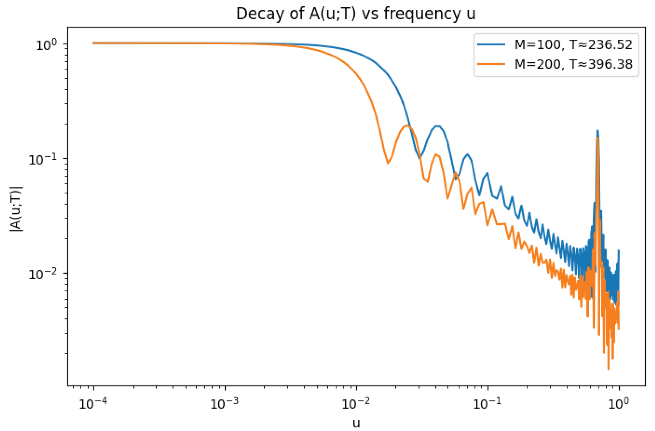
Table 4.
Numerical estimates of pair-correlation decay constants. Here M is the number of zeros used, T the height of the largest zero, , and the fitted exponent from .
Table 4.
Numerical estimates of pair-correlation decay constants. Here M is the number of zeros used, T the height of the largest zero, , and the fitted exponent from .
| M | T | N | ||||
|---|---|---|---|---|---|---|
| 100 | 236.52 | 100 | 0.6 | 0.361 | 0.173 | 1.032 |
| 100 | 236.52 | 100 | 0.8 | 0.257 | 0.173 | 1.032 |
| 100 | 236.52 | 100 | 1.0 | 0.183 | 0.173 | 1.032 |
| 200 | 396.38 | 200 | 0.6 | 0.342 | 0.151 | 1.057 |
| 200 | 396.38 | 200 | 0.8 | 0.239 | 0.151 | 1.057 |
| 200 | 396.38 | 200 | 1.0 | 0.167 | 0.151 | 1.057 |
Table 6.
Summary of tunable parameters in the entropy–sieve method.
| Param. | Role | Typical choice | Trade-off |
|---|---|---|---|
| Truncation length | –8 (polylog) | Larger A: smaller remainder, harder moments | |
| Approx. failure set | Bigger B ⇒ bigger A | ||
| Low-entropy set | Block length | Larger m: better entropy, costlier cumulants | |
| C | Remainder tolerance | –3 | Larger C: stronger control, bigger A |
| B | Power-saving exponent | –10 | Larger B: bigger A or higher moments |
| Small-gap sieve rate | –2 | Larger : faster decay, limited by MGF | |
| MGF tail rate | , | Fixed by X, controls linear tail | |
| m | Entropy block length | slowly | Larger m: smaller entropy set, more cost |
Disclaimer/Publisher’s Note: The statements, opinions and data contained in all publications are solely those of the individual author(s) and contributor(s) and not of MDPI and/or the editor(s). MDPI and/or the editor(s) disclaim responsibility for any injury to people or property resulting from any ideas, methods, instructions or products referred to in the content. |
© 2025 by the authors. Licensee MDPI, Basel, Switzerland. This article is an open access article distributed under the terms and conditions of the Creative Commons Attribution (CC BY) license (http://creativecommons.org/licenses/by/4.0/).
Copyright: This open access article is published under a Creative Commons CC BY 4.0 license, which permit the free download, distribution, and reuse, provided that the author and preprint are cited in any reuse.


