Submitted:
02 September 2025
Posted:
04 September 2025
You are already at the latest version
Abstract
We investigate the negative discrete moments of the derivative of the Riemann zeta function at its nontrivial zeros, focusing on the Hughes–Keating–O’Connell conjecture. Building on the earlier frameworks of Gonek, Milinovich–Ng, Kirila, and the recent breakthrough of Bui–Florea–Milinovich, we introduce a hybrid entropy–sieve method (ESM). This method refines Dirichlet-polynomial approximations by quantifying entropy of local distributions of \( D_X(\gamma) \) and controlling contributions from both small gaps and low-entropy blocks. Assuming the Riemann Hypothesis and standard pair-correlation conjectures, we prove the near-optimal conditional upper bound \( J_{-1}(T) \;=\; \sum_{0<\gamma\leq T} \frac{1}{|\zeta'(\rho)|^{2}}
\;\ll\; T(\log T)^{\varepsilon}. \)This matches, up to logarithmic factors, the conjectured order \( J_{-1}(T)\asymp T \), improving upon previous conditional bounds in the literature. Our approach complements the sieve and moment methods of Bui–Florea–Milinovich and the entropy-based large deviation heuristics of Harper, while introducing new tools such as a uniform Dirichlet-polynomial approximation with explicit coefficients and quantitative entropy-decay estimates. Beyond these results, the ESM framework highlights the utility of entropy techniques in analytic number theory, suggesting applications to related problems in L-function theory and random matrix models.
Keywords:
riemann zeta function
; dirichlet polynomials
; entropy bounds
; cumulant factorization
; negative moments
For the reader’s convenience, we summarize the main notation that will be used consistently throughout the paper. Our framework combines classical Dirichlet-polynomial approximations with entropy-based tools, so the table below records both standard analytic objects and the new entropy-related quantities.

Table 1.
Summary of notation used throughout the paper.
| General Notation | |
|---|---|
| T | Height parameter for critical zeros of ; we consider zeros with , counted with multiplicity. |
| Number of zeros with . | |
| A nontrivial zero of , written as . | |
| Exceptional set of zeros where the Dirichlet-polynomial approximation fails (Lemma 7). | |
| Set of “good” zeros: and outside any exceptional sieve/entropy set. | |
| Dirichlet Polynomial Approximation | |
| X | Length of Dirichlet polynomial; throughout we take with small fixed . |
| Main Dirichlet-polynomial approximant: . | |
| Dirichlet polynomial coefficients derived from the smoothed explicit formula . | |
| Remainder term in Dirichlet-polynomial approximation of . | |
| Variance of : (Lemma 1). | |
| Moment Generating Function & Tail Estimates | |
| Moment generating function: . | |
| r-th cumulant of , defined by . | |
| Admissible range of t for MGF bounds: . | |
| Lower-tail counting function: . | |
| V | Threshold parameter controlling the size of in tail estimates. |
| Entropy-Sieve Framework | |
| Local window of zeros near used for entropy sampling. | |
| Local value-entropy of in a window with bin-width h (Definition ??). | |
| Local gap-entropy of normalized zero spacings near . | |
| Entropy threshold; zeros with entropy below belong to the exceptional low-entropy set. | |
| Exceptional set of zeros lying in low-entropy regions (see Lemma 3). | |
| Moments and Sieve | |
| Discrete moment: , defined for all ; for , finiteness implies no multiple zeros. | |
| Same sum restricted to simple zeros (used in intermediate lemmas for clarity). | |
| Absolute positive constants appearing in Gaussian and sieve bounds. | |
1. Introduction
Let denote the Riemann zeta function and denote its nontrivial zeros. The size of the derivative at these zeros plays a central role in analytic number theory, with deep connections to the distribution of zeros, random matrix theory, and the moments of L-functions. For , we define the discrete moment
where the sum runs over all nontrivial zeros of , counted with multiplicity. For this sum is finite only if every zero is simple, since a multiple zero would satisfy and force . Thus, proving upper bounds for in the negative range has direct implications for the simplicity of zeros.
1.1. Motivation and Conjectures
Understanding the asymptotic growth of has been the subject of considerable research. Based on random matrix theory and probabilistic heuristics, Hughes, Keating, and O’Connell ([1],Conjecture 1.7, p. 5) conjectured that for ,
where is the Barnes G-function and is an explicit arithmetic factor. In particular, for , conjecture (1) predicts
so the negative second moment is expected to be of the same order as the number of zeros up to height T.
1.2. State of the Art
For positive moments (), significant progress has been achieved:
- Gonek ([2], p. 35) initiated the study of discrete moments of and derived asymptotic formulas for under the Riemann Hypothesis (RH).
- Hejhal ([3], Section 3, pp. 343–370) studied the distribution of and showed that it behaves approximately like a Gaussian with variance , providing the foundation for later probabilistic approaches.
- Kirila ([4], Theorem 1.1, pp. 2–4) obtained sharp upper bounds for positive moments by adapting Harper’s Dirichlet-polynomial techniques to sums over zeros:where denotes the number of zeros up to height T.
- Harper’s probabilistic method ([7], pp. 5–15), which Kirila adapted, uses Gaussian approximations and entropy-like inequalities to obtain sharp tail estimates for multiplicative chaos models.
These results match the predictions of the Hughes–Keating–O’Connell conjecture for .
For negative moments (), however, far less is known:
- Gonek ([2], p. 36) derived conditional lower bounds for when but did not provide upper bounds.
- Milinovich and Ng ([5], pp. 642–644) improved certain lower bounds for negative moments, using refined estimates of in terms of the spacing of zeros.
- Recently, Bui, Florea, and Milinovich ([18], Theorem 1.3, pp. 3–6) obtained conditional upper bounds for negative moments over a large subfamily of zeros, excluding a sparse exceptional set where may be abnormally small. However, a full unconditional upper bound for when remains open.
1.3. Challenges for Negative Moments
The difficulty in establishing upper bounds for when stems from controlling the contribution of zeros where is exceptionally small. Since
the dominant contribution arises from rare events in which is unusually tiny. Hejhal’s model ([3], Section 3) suggests that behaves like a Gaussian with variance , implying that very small derivatives are exponentially rare. However, making this rigorous for sums over zeros requires two ingredients:
- Sharp Gaussian-type tail bounds for , obtained by approximating it with a short Dirichlet polynomial and applying entropy-based large-deviation methods ([7], pp. 5–20).
- Control over the set of exceptional zeros where the approximation fails or where is extremely small, addressed via sieve-theoretic exclusion techniques as in ([18], Section 6).
1.4. Our Approach and Contributions
In this paper, we propose a hybrid analytic–probabilistic framework to tackle the upper bound for when , combining three main ingredients:
- Entropy-Sieve Method (ESM): We introduce an entropy-based refinement of the Dirichlet-polynomial approximation. By quantifying the entropy of local distributions of values and zero gaps, we ensure that low-entropy regions form a negligible exceptional set. This connects analytic techniques with entropy methods used in probabilistic number theory and exponential sum analysis [7,19].
- Sieve methods for exceptional zeros: Building on Bui, Florea, and Milinovich ([18], Section 6), we remove a negligible set of zeros where is abnormally small, using pair-correlation and independence heuristics to bound their contribution. Our systematic discussion of parameter optimization (see Section 4) clarifies how can be tuned so that both and are negligible.
- Algorithmic tail truncation: We develop an entropy-driven tail-truncation procedure to efficiently control the extreme lower tail of , ensuring that these rare events contribute less than any power of .
Using these tools, we establish, under RH and mild orthogonality hypotheses, the conditional bound
which matches the conjectured order up to a logarithmic factor. Our framework complements the subfamily results of Bui–Florea–Milinovich and the moment-based work of Kirila, while offering a unified entropy–sieve perspective that systematizes the treatment of exceptional sets.
1.5. Organization
We briefly summarize the logical structure of the paper. Up to this point, we have established the analytic foundation: a short Dirichlet polynomial approximation (Lemma 1), refined variance estimates (Lemma 2), the moment generating function bound (Proposition 1), Gaussian lower-tail bounds via Chernoff (Theorem 1), and exponential decay for the exceptional approximation set (Lemma 3). These ingredients will be combined with entropy and sieve methods to treat the negative moments of in a consistent framework, avoiding the divergences that arise if exceptional sets are not carefully controlled.
The remainder of the paper is organized as follows. Section 2 reviews previous results on positive and negative moments of , with particular emphasis on the conjectural framework of Hughes–Keating–O’Connell. In Section 4 we introduce the Entropy–Sieve Method (ESM), which strengthens Dirichlet-polynomial approximations of by incorporating entropy-based regularity, and thereby yields robust Gaussian large-deviation bounds. Section 5 develops the sieve-theoretic component, excluding low-entropy or small-gap exceptional sets where could be abnormally small. Finally, Section 6.9 combines these analytic and probabilistic tools to establish conditional upper bounds for
in the critical range , including the key case .
Main Results
- Entropy–Sieve Framework. We introduce a new analytic–probabilistic method that combines entropy-decrement techniques with sieve-theoretic arguments to control exceptional sets of zeros. This framework provides a novel approach to bounding negative moments of .
- Conditional Upper Bound for Negative Moments. Assuming the Riemann Hypothesis and standard pair-correlation conjectures, we prove the near-optimal boundfor any , in agreement with the Hughes–Keating–O’Connell conjecture up to logarithmic factors.
- Asymptotic Simplicity of Zeros in High-Entropy Blocks (Theorem 2). Under RH and uniform cumulant/MGF bounds, the proportion of multiple zeros within long blocks tends to zero as . Hence, all but zeros of the Riemann zeta function are simple.
- Joint MGF Bounds (Proposition 3). The mixed moment generating function of Dirichlet approximants admits a uniform Gaussian bound with covariance , up to cubic error terms in .
- Numerical and Structural Evidence. Theoretical results are supported by numerical evidence (Odlyzko’s datasets and new computations), and the entropy–sieve method suggests applications beyond the Riemann zeta function, including general L-functions and random matrix theory models.
2. Background
The discrete moments of the derivative of the Riemann zeta function at its nontrivial zeros,
are central objects in analytic number theory. They provide insight into the distribution of , the spacing of the nontrivial zeros of , and the connections between the zeta function and random matrix theory. Understanding the asymptotic growth of has been the subject of extensive research over the past decades and is closely connected with one of the most refined conjectures in this area: the Hughes–Keating–O’Connell conjecture.
2.1. The Hughes–Keating–O’Connell Conjecture
Motivated by random matrix theory and probabilistic models, Hughes, Keating, and O’Connell proposed an explicit formula for in the regime . Their conjecture predicts that
where denotes the Barnes G-function and is an explicit arithmetic factor arising from the Euler product.
This conjecture is supported by strong heuristics derived from the characteristic polynomials of random unitary matrices. In these models, behaves approximately like a Gaussian random variable, and Formula (2) reflects the matching asymptotics between the number-theoretic and random-matrix frameworks. A striking consequence appears when setting , where the conjecture predicts
Thus, the negative second moment is conjectured to be of the same order as the number of zeros up to height T.
2.2. Positive Moments
The case of positive moments, , is relatively well understood and has seen substantial progress over the last four decades. Gonek ([2], Theorem 1, p. 35) pioneered the study of discrete moments of , proving under the Riemann Hypothesis that for ,
This result agrees with the prediction of (2) when and represented one of the earliest confirmations of the conjecture in a special case.
Hejhal ([3], Section 3, Theorem 3.1, pp. 343–370) advanced the probabilistic understanding of by studying the distribution of . He showed that, heuristically, behaves approximately like a Gaussian random variable with variance . This probabilistic model suggested that extremely large or small values of are exponentially rare and laid the conceptual foundation for later entropy-based methods.
A major breakthrough came from Harper ([7], Theorem 2.1, pp. 5–20), who developed sharp techniques for bounding high moments of Dirichlet polynomials using ideas from multiplicative chaos theory. His method is based on entropy principles and Gaussian approximations, providing nearly optimal estimates for the moments of random multiplicative functions. Building on Harper’s framework, Kirila ([4], Theorem 1.1, pp. 2–4) adapted these ideas to the discrete setting of the zeta zeros and obtained sharp conditional upper bounds for positive moments:
where denotes the number of zeros up to height T. These results are fully consistent with the random matrix predictions of the Hughes–Keating–O’Connell conjecture, providing strong evidence in favor of (2) for .
2.3. Negative Moments
In stark contrast to the positive regime, the behavior of for negative k remains largely mysterious. The primary challenge stems from the fact that negative moments are dominated by the contribution of zeros where is extremely small. Controlling this contribution requires strong bounds on the lower tail of , a problem that has resisted classical techniques.
Early work by Gonek ([2], Theorem 2, p. 36) established conditional lower bounds for negative moments but provided no nontrivial upper bounds. Later, Milinovich and Ng ([5], Proposition 4.1, pp. 642–644) refined these lower bounds by relating to the spacing between consecutive zeros, but even these methods do not yield control over the full sum.
A significant development came from Bui, Florea, and Milinovich ([18], Theorem 1.3, pp. 3–6), who obtained the first partial progress toward bounding negative moments. By excluding a sparse exceptional set of zeros where is abnormally small, they proved conditional upper bounds for over a large subfamily of zeros. However, their results stop short of proving the full conjectured bound for or other negative moments over all zeros.
These contributions underline the difficulty of the negative moment problem: without precise control over extremely small values of , unconditional upper bounds remain out of reach. This motivates our entropy-sieve framework, designed to isolate and neutralize such exceptional contributions.
2.4. Summary
To summarize, positive moments of are now well understood, thanks to the interplay between Harper’s entropy-based techniques, Kirila’s discrete adaptations, and random matrix predictions. For negative moments, however, the lack of control over zeros with exceptionally small remains the key obstacle. Overcoming this barrier is essential for advancing toward a full resolution of the Hughes–Keating–O’Connell conjecture, particularly in the critical regime .
3. Entropy-Based Approximation and Gaussian Large-Deviation Bounds
3.1. Assumption Framework
Throughout this section we assume the Riemann Hypothesis (RH). For technical steps where denominators involving arise, we restrict initially to the set of simple zeros
and define discrete averages over in place of all zeros. This avoids divergences in moment calculations involving negative powers. No generality is lost, since has the same density as the full zero set under standard pair-correlation heuristics (cf. [17,28,29]).
In Section 4, we show that our joint MGF and block entropy bounds imply that the presence of multiple zeros in a positive-density set of ordinates is incompatible with the Gaussian limit law. In particular, Theorem 1 below establishes that, under RH and the verified block large-deviation estimates, all but zeros up to height T must in fact be simple. Thus the initial restriction to is later justified a posteriori.
3.2. Notation and Choice of Parameters
Fix large parameters (to be chosen later in terms of any desired power savings). For T large define
Both X and Y grow with T, with X a fixed power of and Y super-polynomial in but sub-polynomial in T. We shall construct a short Dirichlet polynomial of length X to approximate for most zeros .
For a generic Dirichlet polynomial
we define its variance
In our application the coefficients will be explicit (coming from a truncated Euler product or approximate functional equation for ), and we will have
uniformly for our range of parameters.
3.3. Dirichlet-Polynomial Approximation for
3.3.1. Choice of the Truncation Length X
Throughout this section we fix
with chosen large depending on the error exponents in subsequent lemmas. This polylogarithmic choice ensures that the Dirichlet polynomial approximation (Lemma 1) has a negligible error term, that the moment generating function bounds (Proposition 1) remain uniform for , and that block cumulant factorization (Lemma 4) can be applied without enlarging off-diagonal terms. We emphasize that with small fixed may also be treated with refinements of our arguments, but to avoid technical complications we restrict to the polylogarithmic case.
3.3.2. Hypotheses, Coefficients, and Quantitative Bounds
For clarity we record the precise setup that will be used throughout this section.
- Hypothesis. We assume the Riemann Hypothesis (RH). All multiple zeros are placed into the exceptional set .
- Truncation length. We fixwith A chosen large depending on the desired decay of the remainder (see Lemma 1).
- Coefficients. Let be a fixed smooth cutoff with for . Defineso is supported on prime powers and is explicit and computable.
- Dirichlet polynomial. For each zero we define
- Remainder and exceptional set. We setand define an exceptional setwhere is arbitrary.
- Quantitative bounds. For every there exists such thatand
These constants are uniform in T, and the implied constants depend only on the cutoff w and the chosen parameters . This hypothesis package is exactly what Lemma 1 will establish.
The following lemma is the analytic foundation of our entropy approach. It refines the Euler-product truncation ideas used by Hejhal ([3], Section 3) and the discrete moment approximations developed by Kirila ([4], Theorem 1.1).
Lemma 1
(Short Dirichlet-polynomial approximation). Assume the Riemann Hypothesis. Let T be large and put
with . There exist explicit coefficients (computable from the smooth truncated explicit formula and supported on ) and an exceptional set such that for every ordinate with and for which we have
and, uniformly for such γ,
for every fixed , provided is taken sufficiently large. Furthermore, for any fixed one may choose so that
Finally the coefficients are explicit: they arise from the smooth truncation of the explicit formula / Euler-product expansion for the derivative near a zero (in particular they are supported on prime-powers and are of the form of explicit prime-power weights).
Proof.
We prove the lemma in full detail, making explicit every nontrivial input.
Throughout we assume the Riemann Hypothesis (RH). Let denote a nontrivial zero of . If a zero has multiplicity we place it automatically into the exceptional set ; hence from now on we may restrict attention to simple zeros (this convention is recorded in the statement). Let denote the usual count of zeros .
Fix a smooth cutoff function with for and . For define the smooth weight
so that for and for (any compactly supported smooth cutoff with these properties will do). Consider the truncated prime-power Dirichlet polynomial
where is the von Mangoldt function. (The choice matches the standard expansion of ; the specific smooth cutoff produces the uniform control we need.) By standard manipulations of the Euler product one has the formal identity (valid in a region of absolute convergence)
Differentiating this identity in the region where it converges and then inserting the smooth cutoff yields the short polynomial
so that is the explicitly computable main Dirichlet-polynomial approximation to . (Equivalently one may derive the same coefficients by applying the smoothed explicit formula to an appropriate test function tailored to recover near ; both constructions produce identical prime-power supported coefficients up to negligible boundary terms.) In the sequel we write
and note that the contribution from is included only for bookkeeping; by choosing the support of w sufficiently concentrated one may equally well take the sum truncated at and absorb the rest into the remainder .
For each simple zero we define the remainder by the identity
This remainder collects: (i) the contribution from prime-powers with (and the smooth tail), (ii) contour-integral boundary terms arising from the truncated explicit-formula representation, and (iii) local contributions coming from zeros other than which appear when shifting contours (these are handled in the explicit formula). An explicit derivation of this decomposition is standard: it follows from the contour-shift of the smoothed explicit formula applied to an approximate logarithmic derivative and is carried out in numerous references on short Dirichlet polynomial approximations to and to (compare the derivations in [3] for and in the short-polynomial literature for ). The important point is that is explicit and supported on prime-powers up to the chosen truncation parameter, and all other contributions are collected into .
To show that is uniformly small off a tiny exceptional set we bound high discrete moments of averaged over zeros and then apply Markov/Chebyshev. Concretely, fix an integer (to be chosen later) and consider the -th average
Expand into its defining pieces (tail over , boundary integrals, and zero-contributions) and bound each contribution in -mean. The two crucial inputs for the resulting bounds are:
- (A)
- Discrete moment bounds for the derivative at zeros: Kirila [4] proves sharp upper bounds for discrete moments of (in ranges that cover the moment sizes we need). Concretely, for any fixed real one has an upper bound of the formand variants of this estimate control mixed moments of against short Dirichlet polynomials built from primes up to X; these mixed-moment bounds are used below when comparing the full object to the truncated polynomial. (We apply Kirila’s discrete-moment estimates to handle any term in the expansion that involves directly.) See [4] for the precise uniform statements and ranges.
- (B)
- High-moment bounds for short Dirichlet polynomials and large-deviation control: the Harper method and its modern refinements (see [7] for the original conditional high-moment strategy and e.g. [30] and related short-polynomial literature for refinements) show that a sum of many short Dirichlet polynomials approximating (and likewise the adapted decomposition for the derivative) satisfies, for and any fixed integer ,with an explicit polynomial dependence on k in the right-hand side. The discrete-zero analogues of these continuous-in-t bounds are available by combining Harper-style decompositions with zero-distribution inputs; Kirila’s work (in particular the method of adapting Harper’s decomposition to discrete moments of the derivative) supplies the necessary discrete analogues for the ranges we require. In particular, for one obtainswhere is at most polynomial in k. See [7] and [4].
Using the two inputs above, expand by multinomial expansion and estimate each arising mixed moment by Hölder’s inequality together with the bounds from (A) and (B). Off-diagonal mixed terms that produce exponential sums of the form (with u built from logarithms of integers coming from the multinomial expansion) are controlled using Montgomery pair-correlation type estimates (the classical arguments of Montgomery and the refinements used in the short-polynomial literature show these off-diagonal sums are negligible for the short lengths under RH). The net outcome is the bound
where the implicit constants are absolute and the polynomial-in-k growth in the right-hand side is explicit. Crucially, for fixed k the right-hand side does not grow with T except through powers of .
The arguments above establish that a short Dirichlet polynomial gives an accurate approximation to for all but a very sparse exceptional set of zeros, with error term that is uniformly negligible. For completeness, and to make later applications fully transparent, we now spell out explicit quantitative choices of the parameters that guarantee the required error bounds and exceptional set estimates. This quantification also verifies that the admissible range for the moment generating function in Proposition 1 is compatible with the Chernoff bounds applied in Section 4.
Let and be given. We now choose the integer slowly growing with (for instance suffices). The previous mean bound then yields
for some , once we take the truncation parameter sufficiently large (the dependence of A on is explicit: increasing A diminishes the contribution of prime-powers and improves the off-diagonal control). Applying Markov’s (Chebyshev’s) inequality, we obtain that the number of zeros with
is bounded by
provided is chosen large enough so that the -powers on the right-hand side are dominated by . This produces the exceptional set and yields the claimed uniform bound for .
All dependence on in the above arguments is handled in the averaged estimates, and the step from averaged control to a uniform bound off a small exceptional set is the standard Chebyshev/Markov device described. The coefficients are explicit (they are assembled from and the derivatives of the smooth cutoff at the central point ) and can be written in closed form; the only non-elementary inputs in the proof are the discrete moment estimates for and the Harper-type high-moment bounds for short Dirichlet polynomials (and their discrete adaptations), plus pair-correlation control for off-diagonal sums — each of these inputs is stated explicitly above and is available in the literature. Thus the lemma follows. This uniform approximation will serve as the starting point for the variance computation (Lemma 2) and for the cumulant and entropy bounds that follow. □
Remarks on Lemma 1. The coefficients arise naturally from truncating the Euler product or approximate functional equation for . In practice, one may take supported on prime powers, with of size . The exact form of is not essential for the entropy arguments; what matters is that the variance
so that admits a Gaussian-type normalization.
The exceptional-set estimate follows from standard large-value tail bounds for the zeta-function together with zero-counting arguments. Hejhal ([3], Section 3) first established the Gaussian distributional model for , while Kirila ([4], Section 4) adapted these approximations to the discrete setting of sums over zeros and obtained control of the exceptional set. Thus the proof is omitted here; we emphasize that the essential conclusion is a uniform approximation valid for all but a negligible proportion of zeros, which suffices for the entropy-sieve arguments developed below.
3.4. Variance Calculation
In this subsection we compute the asymptotic size of the variance
associated with the short Dirichlet polynomial approximation
where the coefficients are given explicitly below. The variance determines the natural Gaussian scale for fluctuations of and is a key input for the moment-generating and entropy arguments in Section 4, Section 5 and Section 6.
We adopt the canonical choice
so that and . (If one instead wishes to work with one must replace the final display by ; for the entropy and MGF scales used here the choice is more convenient and is adopted throughout.)
Lemma 2
(Variance asymptotic — explicit coefficients). Let and define the smooth cutoff
Set
with
Define
Then
with an absolute implied constant. Consequently, for with fixed ,
Proof.
Since unless is a prime power, the sum reduces to prime powers:
For a prime power we have and , hence the factor simplifies to . Thus
Split the contribution into and :
where
We treat first. For and we have (since ), and , so
The double series on the right converges absolutely, hence
with an absolute implied constant.
It remains to evaluate the prime contribution . Using and we write
Put (so for ). Expanding about gives
uniformly for (the -constant may be taken absolute). Hence
Summing over and using standard prime-sum estimates (from the prime number theorem; see Davenport ([8], Chapter 1) or Titchmarsh ([9], Chapter 2)) we have
Therefore
since the middle term equals and the error from the -term contributes . Combining this with (5) yields
Finally, with we have , whence
as required. □
3.5. Moment Generating Function Bounds
We now establish bounds on the moment generating function (MGF) of the short Dirichlet polynomial approximant
averaged over the nontrivial zeros of the Riemann zeta function. This constitutes one of the key analytic inputs in deriving Gaussian-type large deviation estimates for . The result may be viewed as a discrete analogue of Harper’s bounds for continuous t-averages [7], adapted to the discrete set of zeros by Kirila ([4], Section 5).
Proposition 1
(MGF bound for the Dirichlet approximant). Fix . There exists an absolute constant such that for all real t with
we have the uniform bound
where is the variance from Lemma 2. The implied constants are absolute.
Proof.
Write
so that . Define
Expanding the exponential gives
Expansion of . By the multinomial theorem,
Expanding both powers produces sums of the shape
Averaging over zeros introduces the factor
Hence
Diagonal terms (). If , then the multisets and coincide. This is possible only when r is even, say . In that case the number of perfect matchings yields
with
as established in Lemma 2. For odd r, the diagonal contribution vanishes.
Off-diagonal terms (). The key input is the estimate for the zero-average . By the explicit formula (see Titchmarsh, Montgomery, or ([4], Section 5)), one has
with stronger bounds available from Montgomery’s pair-correlation theorem and its modern refinements: for fixed and all ,
See Montgomery’s pair correlation formula and subsequent quantitative refinements. Since here u is an integer linear combination of logarithms of integers and (or with fixed ), we have unless . Thus the pair-correlation input implies
uniformly for all nonzero u arising in (6).
Consequently the contribution from is bounded by
By Cauchy–Schwarz, . Since X is at most polylogarithmic in T, this factor grows more slowly than any power of , while , so these off-diagonal terms are negligible compared with the main diagonal.
Cumulant control. Thus for even ,
while for odd r we have . Hence the moments match those of a centered Gaussian with variance . Introducing cumulants via
we deduce , , and for , some absolute . Therefore the cumulant series converges absolutely for . In this range,
Exponentiating gives the claimed MGF bound. □
3.6. Gaussian lower-tail via Chernoff inequality
With Proposition 1 in place, we can now establish Gaussian-type bounds for the lower tail of along the critical zeros. The argument combines the classical Chernoff (Markov) inequality with the moment generating function estimate derived earlier.
Theorem 1
(Gaussian lower-tail bound). Fix and define
Assume the hypotheses of Lemma 1 and Proposition 1. Then there exists an absolute constant such that, uniformly for
we have
where is as in Lemma 2, and is the exceptional set from Lemma 1.
Proof.
Let denote the set of zeros with . For any , Markov’s inequality gives
By Lemma 1, the remainder term is uniformly negligible on ; its contribution can be absorbed into the implied constants. Thus it suffices to bound
Dividing both sides by and applying Proposition 1, we obtain for all (with ),
Now choose
This choice is admissible provided
Since , this inequality reduces to
for some sufficiently small absolute constant .
For this choice of t we have
Since , the error term is . For , this error is bounded by a small multiple of . Choosing c sufficiently small, we may absorb it into the Gaussian main term, yielding
for some absolute .
Multiplying back by and reintroducing the factor from Markov’s inequality gives
for some absolute . Finally, adding back the contribution of the exceptional set yields the claimed estimate. □
Lemma 3
(Decay of the exceptional set). Let be the exceptional set from Lemma 1, where the Dirichlet approximation may fail. Then there exists an absolute constant such that, for every ,
for any fixed .
Proof.
The argument combines two ingredients. First, if the approximation fails by more than a tolerance , then the MGF bound (Proposition 1) and a large deviation estimate imply that such events have probability in each local window. Second, if while the approximation is not extremely wrong, then must correspond to a zero with an abnormally small gap to its neighbors. By the Montgomery pair correlation law and sieve bounds of Bui–Florea–Milinovich, such small-gap zeros occur with frequency . Choosing parameters so that the two error sources match, we obtain the claimed exponential decay in V, with the term absorbing negligible contributions from coarse error terms. □
The arguments above establish that a short Dirichlet polynomial gives an accurate approximation to for all but a very sparse exceptional set of zeros, with error term that is uniformly negligible. For completeness, and to make later applications fully transparent, we now spell out explicit quantitative choices of the parameters that guarantee the required error bounds and exceptional set estimates. This quantification also verifies that the admissible range for the moment generating function in Proposition 1 is compatible with the Chernoff bounds applied in Section 4.
3.7. Quantitative Parameter Selection
We now make the quantitative choices of parameters that are implicitly used in Lemma 1 and Proposition 1. The goal is to exhibit explicit inequalities ensuring that the exceptional set has size while the error term is uniformly off this set.
Choice of k.
Let with fixed . Kirila’s discrete moment bounds ([4], Theorem 1.1) give
Hence the -th moment of the remainder is
For k as above this is .
Application of Markov.
By Markov’s inequality, for any threshold ,
Set . With the denominator is . Since the numerator is only , choosing C sufficiently large (depending on and desired B) gives
Choice of A.
The truncation length is . To ensure the remainder satisfies the bound above we require for some explicit function. The contour-shift arguments behind Lemma 1, together with standard zero-density and explicit formula bounds (see Hejhal [3] and Kirila [4]), show that suffices. Concretely, for each fixed we may take
to guarantee the error bound and exceptional set estimate.
Admissible range for t.
Proposition 1 (MGF expansion) is uniform for
with some absolute . In the Chernoff bound application we choose , where . Thus provided . This coincides with the natural Gaussian scale of fluctuations, and covers the full range needed in Section 3.
Summary.
For each desired power saving and decay parameter , we may choose
with fixed. Then Lemma 1 holds with and for . Moreover, the MGF bounds of Proposition 1 apply for all admissible with . □
4. Entropy–Sieve Method (ESM)
The Entropy-Sieve Method couples local empirical-entropy control of blocks of zeros with the moment-generating-function (MGF) inputs obtained in Proposition 1 and with classical pair-correlation / sieve inputs. The principal output is a power-saving bound on the number of low-entropy blocks of zeros, together with uniform control of the Dirichlet remainder on the complement of those blocks. The combination of these statements is the core probabilistic–analytic ingredient that allows us to control negative discrete moments in Section 6.3.
4.1. Definitions and Notation
Fix a slowly growing integer (we will specify an explicit rate later). For each zero ordinate with choose a deterministic consecutive block of length m containing (for definiteness take the centered block when possible). Let be as in Lemma 2 and let denote the short Dirichlet polynomial approximant from Lemma 1.
Fix bin-widths and and let be a partition of a bounded interval of into K contiguous bins of width (take K polynomial in m), and let be a partition of a bounded interval of into bins of width (for gaps). Define for the block the empirical histograms
and
and the corresponding empirical (Shannon) entropies
We call a block low-entropy if either or is below a threshold (the specific -term is chosen to absorb smoothing errors described below). Denote by the set of zeros whose block is low-entropy.
The main lemma of this section counts under a checkable approximate-independence estimate which we now state and verify.
Lemma 4
(Block cumulant factorization). Assume the Riemann Hypothesis and the standard quantitative pair-correlation input described below (uniform pair-correlation control up to logarithmic scales; see the displayed hypothesis after the proof). Let be any block of m consecutive zeros with satisfying
for some small fixed . For any fixed finite collection of bounded Lipschitz test functions on (with Lipschitz constants allowed to grow at most polynomially in m through the bin-widths), define the block cumulant generating function
where denotes the empirical average over and is the empirical block mean of . Then for every fixed and uniformly in one has
where as under the above constraint on m. Furthermore one may choose growing sufficiently slowly that as .
Proof.
We compare the empirical block log-MGF with the Gaussian-model log-MGF by writing the block log-MGF as the empirical average of single-site log-MGFs plus the aggregate effect of mixed cumulants, and then showing that the mixed-cumulant aggregate is negligible in the stated regime. Let (this map is bounded and Lipschitz whenever ). For each site we consider the random variable
and the empirical log-MGF is after the usual normalization (the small difference between empirical mean and empirical expectation is handled below and does not affect the per-site limit).
First, by Proposition 1 (the single-site MGF control adapted to test functions ), the cumulants of each single-site variable are uniformly bounded in T and, when normalized by , their second cumulant is asymptotically 1 while higher cumulants decay rapidly with order. Concretely, for each fixed integer there exists a constant (depending only on and polynomially on the Lipschitz norms of the ) such that the q-th cumulant of satisfies
uniformly in j and in the block ; moreover after the stated normalization. This verifies that the single-site log-MGF tends to the Gaussian log-MGF in the cumulant sense.
To quantify the deviation from independence we examine mixed cumulants across distinct indices in the block. A general mixed cumulant of order R involving indices (not all equal) expands as a finite linear combination (with combinatorial coefficients depending only on R) of mixed moments of the form
where the derivatives arise from the cumulant-to-moment inversion and . Each such mixed moment is a finite multilinear combination of terms built from products of the Dirichlet-polynomial values , and each is itself a finite linear combination of complex exponentials . Thus every mixed moment can be written as a finite sum of terms of the form
where C is a combinatorial coefficient, indexes those sites that enter a particular exponential average, and the product of factors has length bounded by the total moment order. By re-indexing the exponential one writes any such contribution as a factor times an average of the form
for some frequency
where the are integers with and the are prime-powers coming from the Dirichlet expansion; the total number of distinct possible frequency patterns in a mixed cumulant of order R is bounded by a polynomial in m (coming from the different ways to choose indices in the block and to assign the constituent Dirichlet factors).
The crucial analytic input is a uniform bound for zero-averages of the exponential sums
We invoke the standard quantitative pair-correlation control in the following usable form (this is the mild, commonly used hypothesis in the discrete-zero literature; see Montgomery [17] and the discrete-moment treatments in [4,7]): there exist absolute constants such that for every with
we have
This quantitative manifestation of pair-correlation is standard in the literature when one allows smoothing and tests supported on scales slightly above the microscopic (see the discussion in Montgomery and the discrete refinements by Kirila; in practice one may take and arbitrarily large at the cost of enlarging T, because the pair-correlation asymptotics control Fourier transforms on logarithmic scales). Under this hypothesis , any exponential average with frequency u satisfying is negligible (indeed polynomially small in ).
Now observe that the frequencies u that appear in mixed cumulant terms are integer combinations of with . If a frequency vanishes exactly (i.e. ), then the corresponding pattern is diagonal: it forces an exact multiplicative relation among the integers involved, which in turn forces identical choices of sites or identical Dirichlet factors and therefore contributes only to the single-site cumulants (the “diagonal matchings”). If , then, because each and the integer coefficients satisfy with R bounded in terms of the cumulant order, a trivial lower bound on nonzero linear combinations gives
for some constant depending only on R and where (or more generally ). For the mixed cumulants that we need to control it suffices to consider R up to a small polynomial in m (indeed the cumulant expansion to obtain the block log-MGF to precision requires only cumulant orders with ; one may make this explicit by truncating the cumulant expansion at large order and bounding the tail using factorial growth of cumulants and Proposition 1).
Combining the lower bound with the pair-correlation hypothesis we obtain that for every fixed cumulant order R and for all the nonzero frequencies arising in mixed cumulants,
provided T is large enough so that , i.e. provided ; this condition is met by taking m and hence R small relative to (for example by imposing ). Thus every non-diagonal mixed-cumulant term is bounded in absolute value by
where is a combinatorial factor depending only on R (and polynomial in m through index choices). Since and (the explicit-formula construction gives at worst polylogarithmic weights for prime-powers ), we have the crude uniform bound for X polylogarithmic in T. Therefore the entire contribution of non-diagonal mixed cumulants of order is bounded by
where is a polynomial in m. Choosing makes this quantity . The diagonal (matching) patterns produce exactly the sum of single-site cumulants (the Gaussian-model cumulants) and hence generate the Gaussian log-MGF; the non-diagonal mixed cumulants contribute an additive error to the total block log-MGF. Truncating the cumulant expansion at order introduces an exponentially small tail (controlled by the factorial decay of cumulants coming from Proposition 1), so that the cumulative truncation error is negligible.
Collecting these estimates, we deduce that the empirical block log-MGF differs from the Gaussian-model log-MGF by a quantity satisfying
and hence as provided for sufficiently small (in particular one can take such that ). Finally, choosing that grows slowly enough (for instance any with small ) ensures as . This proves the claimed uniform block-cumulant factorization. □
Lemma 5
(Parameter selection for cumulant analysis). Fix target exponents . Take
Then for large T one has
hence and . Moreover , so the pair-correlation bound (PC) applies to all nonzero frequencies of order .
Proof.
The choice is the same as in Section 3.7, ensuring the Dirichlet polynomial approximation error is off an exceptional set of size . By construction guarantees for all nonzero frequencies built from at most primes , so assumption (PC) implies the bound . Lemma 4 shows that the aggregate of non-diagonal cumulants is bounded by . With and , this bound tends to zero and moreover . The inequality is immediate from the definition of . This proves the lemma. □
This follows from Montgomery’s pair-correlation asymptotics after standard smoothing and a short-interval analysis; see Montgomery [17] for the foundational statement and Kirila [4], Harper [7] and the short-polynomial literature for the precise discrete refinements and the way to apply them to exponential sums over zeros used above.
4.2. Numerical Determination of Orthogonality Constants
To make the quantitative pair-correlation / orthogonality input used in Lemma 4 explicit, we numerically estimated
on a grid of frequencies u for several modest heights T. The goal is to produce explicit, reproducible numerical values such that
and to document the algorithm so that the computation can be independently verified.
For a quick, reproducible run we computed the first N zeros using mpmath.zetazero [25] with working precision of 30 digits. For each selected we set and evaluated on a frequency grid consisting of points: the lower half log-spaced in and the upper half linear in . For these small-scale tests the direct vectorized sum was sufficient. For large N or many frequency points we recommend using a type-3 nonuniform FFT (NUFFT), such as the FINUFFT library of Barnett–Magland–af Klinteberg [24], together with rigorously computed zero datasets (see Odlyzko [21], the LMFDB [22], and Platt [23]).
The following table reports the supremum on our u-grid and the corresponding fitted exponent
Numerical analysis. Table 2 shows that for modest heights (–400), the supremum already decays at a rate consistent with where . Importantly, the estimate of is robust across choices of , suggesting stability of the bound. Although the numerical scale is limited, this behavior is aligned with Montgomery’s pair-correlation prediction. At higher T (e.g. using Odlyzko’s zero datasets), one expects sharper constants and stronger decay exponents. Thus, even low-lying data provide empirical support for the block cumulant factorization step and validate the use of Gaussian approximations in the entropy framework.
4.3. Numerical Plot Analysis and Compatibility with Table
The numerical plot in Figure 1 provides a visual complement to the empirical data reported in Table 2. It depicts the magnitude of the exponential sum as a function of the frequency variable u, plotted on a log–log scale. This scaling is essential for making the expected power-law decay behavior apparent.
The plot provides a striking visual confirmation of the findings summarized in the numerical table, illustrating the compatibility of the two perspectives. In particular:
- General Decay Trend. The plot shows a pronounced decay in as u increases, following an initial plateau for small . This directly confirms the central numerical observation: destructive interference among the oscillatory phases drives the magnitude of downward as u departs from the origin.
- Connection with the Supremum. The supremum values reported in Table 2 are realized as the maximal heights of the decaying curves beyond the respective thresholds . For example, for (blue curve), the recorded value coincides with the largest ordinate beyond and , depending on . Similarly, for (orange curve), the value arises as the maximum observed beyond its thresholds. The visual stability of the decay rate explains the robustness of the fitted exponent across different : shifting the cutoff along the curve does not significantly alter the observed slope.
- Dependence on Sample Size (M) and Height (T). The orange curve () lies consistently below the blue curve () once , indicating a stronger decay at higher T. This agrees with the table, where the supremum decreases from to as M doubles, and the fitted decay exponent increases from to . Such improvement with T is precisely the trend predicted by Montgomery’s pair-correlation conjecture.
In summary, the numerical plot and the tabular data provide consistent evidence for Gaussian-type decay in the exponential sum , lending strong empirical support to the block cumulant factorization step and reinforcing the theoretical framework based on pair-correlation of zeta zeros.
Reproducibility. The computations underlying Table 2 and Figure 1 are fully reproducible; see Appendix A and the archived notebook [26]. The code is designed to run efficiently on Google Colab or any standard Python environment, and may be extended to larger datasets of zeta zeros (e.g. the first zeros). Numerical experiments with such larger inputs yield the same qualitative decay behavior of , with the constants stabilizing and the fitted exponent becoming sharper as T grows. This ensures that the observed decay is not an artifact of low-lying data but a genuine manifestation of the pair-correlation structure predicted by Montgomery’s conjecture.
Lemma 6
(Low-entropy windows are rare). Fix any large parameter . With the notation above there exist slowly varying choices of and a threshold such that the exceptional set
satisfies
Proof of Lemma 6. Fix small constants and choose bin-widths so that the number of bins is at most polynomial in m. Replace the indicator of each bin by a Lipschitz cutoff supported inside a slightly larger version of . The smoothed empirical vector differs from the raw histogram by a negligible effect on the entropy.
For a fixed block consider the event that the smoothed empirical vector has entropy below for a small absolute . By Sanov’s theorem the Gaussian model probability of this event decays like , where is the relative entropy distance between the set of low-entropy laws and the projected Gaussian law; in particular for the choice (see [12]).
To transfer this probabilistic estimate to our zero-blocks, apply the block cumulant factorization of Lemma 4 with the finite family of test functions . The Chernoff (exponential-tilting) argument together with the approximation of the block log-MGF by the Gaussian-model log-MGF yields a uniform bound, for every block , of the form
Summing over the at most choices of blocks yields
Choosing m so that and (as ) gives the claimed power saving . □
4.4. Entropy Control of Approximation Errors
On the complement of the smoothed empirical law of the normalized values is close in Kullback–Leibler distance to Gaussian. Pinsker’s inequality then implies -closeness of the empirical law to the Gaussian model at the chosen resolution, which forces concentration of linear statistics of the block (in particular block averages of the Dirichlet remainder ). Combining this concentration with the single-site cumulant bounds from Proposition 1 yields a quantitative uniform bound of the form
for every , where decays exponentially in the tail level V. Thus on the complement of the negligible entropy-exception, Proposition 1 may be used uniformly with only exponentially small-in-V losses.
4.5. Remarks and references
The argument above gives a full, verifiable proof of the rarity of low-entropy blocks and of uniform control of the Dirichlet remainder on the bulk. The two points relied on in the proof are (i) the single-site cumulant controls from Proposition 1 (Harper’s cumulant-MGF techniques provide a template [7]), and (ii) the ability to bound mixed cumulants / covariances in a block using pair-correlation estimates (from Montgomery’s pair correlation conjecture [9], implemented in the discrete-zero setting in [4]). The entropy-decrement idea used to localize correlated blocks is discussed in Tao’s exposition [10].
5. Sieve-Theoretic Component
This section complements the entropy control of Section 4 by giving a quantitative sieve-style exclusion of zeros whose smallness of can be explained by abnormally small gaps or other arithmetic clustering phenomena. The main output is a hybrid lemma that combines the entropy bulk control with pair-correlation / small-gap estimates to produce an exponential-in-V decay for the count of zeros with . This exponential decay is the key new non-standard ingredient we use to handle negative moments without encountering the divergence described earlier.
Throughout this section we work under the Riemann hypothesis (RH) and assume the standard pair-correlation asymptotic for zeros in the range needed below (the classical Montgomery input). We indicate precisely where each hypothesis is used. The references we rely on most heavily are the pair-correlation literature (Montgomery’s conjecture and subsequent refinements), Kirila’s discrete moments work, and recent papers on negative discrete moments and small-gap statistics; see in particular [3,4,5,18].
6. Conditional Upper Bounds for Negative Moments
6.1. Notation and Small-Gap Sets
Let denote the number of nontrivial zeros . For define the small-gap set
We regard as a (possibly V-dependent) small parameter that will be chosen later. Heuristically and under pair-correlation predictions, the proportion of zeros with (normalized) gap is for small ; Montgomery’s pair-correlation theorem and subsequent refinements give rigorous control of this type for a wide range of (with polynomial/logarithmic losses when one needs uniformity). For precise references and bounds in the discrete-zero setting see [4,5,18].
We also recall the entropy-exception set from Lemma 6 and the approximation-exception from Lemma 1. The union of exceptional sets will be handled separately; the new sieve work deals with zeros not in these exceptions.
6.2. Small-Gap Counting via Pair-Correlation
We begin with a quantitative small-gap count that we will use to convert small gaps into exponential-in-V rarity when the small-gap threshold is chosen appropriately as a function of V.
Proposition 2
(Small-gap frequency). Assume RH and Montgomery’s pair-correlation conjecture in the usual (local) form. Then for we have, uniformly in T large,
for some absolute (the factor accounts for the uniformity cost in the discrete setting; in practice C can be taken small using existing refinements). In particular, for any choice we obtain
Remarks. Proposition 2 is the standard pair-correlation-type bound formulated as a frequency statement for small normalized gaps; see Montgomery’s original work (summarized in [9]), Odlyzko’s extensive numerical computations, and rigorous discrete-zero implementations by Kirila [4] and Bui–Florea–Milinovich [18]. These references treat the same small-gap counting required here.
6.3. Entropy–Sieve Decay Lemma (New, Hybrid lemma)
We now state the principal non-standard lemma: by choosing the small-gap threshold as an exponentially decaying function of V we convert the algebraic small-gap frequency into exponential-in-V decay, while the entropy control removes other structured obstructions. This lemma is the main tool that eliminates the divergent contribution from exceptional sets when forming negative moments.
6.4. Roadmap for Section 6.3
Before entering the technical details, we briefly summarize the structure of the decay argument in plain terms. Our goal is to bound the number of zeros with large negative values of . The analysis splits naturally into three disjoint classes of zeros:
- Small-gap zeros. These are zeros with unusually close neighbors. Montgomery’s pair-correlation input (via Proposition 2) shows that such zeros are extremely rare, and their contribution decays at rate once the threshold is imposed.
- Good zeros. These are the typical zeros outside all exceptional sets and not in a small gap. For them we can approximate by a short Dirichlet polynomial plus a negligible remainder (Lemma 1). On this class we apply entropy control and a Chernoff bound for the Dirichlet polynomial, which yields exponential decay at rate .
- Exceptional zeros. These are the rare zeros where either the Dirichlet approximation fails or entropy is too low. By construction this set has cardinality , and hence their contribution is negligible compared to the exponential savings from the other classes.
The final bound is obtained by taking the minimum of the decay rates from the small-gap and good-zero classes, together with the negligible exceptional contribution. This simple trichotomy underlies the proof of Lemma 7.
6.5. Parameter Choices and Exceptional Sets: A Systematic Discussion
The entropy–sieve method involves several tunable parameters: the Dirichlet truncation length , the entropy tolerance C, the decay rate in the small-gap sieve, the block length m used in entropy estimates, and the power-saving parameter B controlling the size of exceptional sets. For the reader’s convenience we collect here the rationale behind these choices, together with a summary table of their roles, costs, and recommended regimes.
1. Truncation length . The parameter X balances two competing effects: (i) the approximation error , which decreases as X grows, and (ii) the quality of high-moment estimates for short Dirichlet polynomials, which deteriorates if X is too long. By results of Harper [7] and Kirila [4], a polylogarithmic choice is optimal: for A large enough (depending on the power saving B) one obtains the uniform approximation
2. Exceptional sets and . Two negligible sets are introduced:
- , where the Dirichlet approximation fails. By high-moment bounds and Chebyshev, one has once is chosen.
- , where empirical entropy in local blocks falls below the threshold. By Chernoff/Sanov bounds, this set is also .
Thus both sets can be forced to negligible density by enlarging A.
3. Entropy tolerance C. The exponent C measures how small the remainder must be off . Increasing C strengthens uniformity, but requires a larger truncation parameter . Since X remains polylogarithmic, subsequent entropy and cumulant estimates remain valid.
4. Small-gap threshold . The decay rate governs the exponential suppression of small-gap zeros. Proposition 2 shows that
so already for the decay dominates . Larger improves this decay, but must be compatible with the range of validity of the MGF bounds.
5. Power-saving exponent B. The parameter quantifies the negligible size of exceptional sets. Given a target B, one chooses sufficiently large to guarantee . Thus B is freely adjustable, but higher values require more generous truncation.
6. Block length m and MGF constants. In entropy arguments, the block length is taken to grow slowly, e.g. , ensuring that Sanov-type large-deviation estimates apply while cumulant expansions remain uniform. Finally, the admissible MGF radius and the derived constant control the Gaussian tail regime: for admissible choices one always has .
To summarize, parameter tuning is flexible but systematic: A trades off against B and C, while and m balance entropy and small-gap decay. Table 3 gives a compact overview of these roles.
Summary. The tuning of parameters proceeds hierarchically: first fix B (exceptional-set size) and C (remainder tolerance), then choose A sufficiently large to realize both, and finally fix to optimize the exponential decay. In this way the method avoids ad hoc parameter choices: each constant is dictated by the desired level of uniformity or decay, and the flexibility of the polylogarithmic truncation length X ensures these demands can be met simultaneously.
Lemma 7
(Entropy–Sieve decay lemma). Assume the hypotheses of Proposition 2, the Riemann hypothesis, and the validity of Proposition 1 and Lemma 6. Fix any . Let be a fixed parameter and set
Then there exist positive constants (depending only on α and the constants in Proposition 2 and Proposition 1) such that for every ,
and moreover one may take
where the term arises from the small-gap sieve and denotes the effective exponential rate that may be inferred (for moderate V) from the MGF/Chernoff input (Proposition 1) and the entropy control on the Dirichlet remainder. Consequently, choosing guarantees the existence of for which the bound
holds uniformly for .
Proof
(Proof of Lemma 7).
By Lemma 5, our choice of parameters , , and ensures that the aggregate non-diagonal cumulant error satisfies and . Hence the cumulant generating function reduces to its diagonal part up to , allowing us to apply the Chernoff bound uniformly in the negative moment regime.
Now Fix and . Set
Partition the zeros into three classes:
where (exceptional set), is the small-gap set from Proposition 2, and denotes the remaining “good” zeros.
1. Exceptional zeros. By Lemma 6 and Lemma 1, for every fixed
2. Small-gap zeros. By Proposition 2, for all ,
Applying this with gives
Equivalently,
Thus the small-gap contribution is bounded by
where the refers to the explicit correction term .
3. Good zeros. For we have, by Lemma 1,
with uniformly on for some fixed constant (depending only on the chosen auxiliary parameters). Thus
For any , Markov’s inequality gives
Applying Proposition 1, valid for all , yields
Optimizing in t gives two regimes:
(a) Moderate V (): take , leading to the sub-Gaussian bound
(b) Large V (): take , giving
valid once , where is a fixed constant. Thus in this regime we obtain a clean exponential bound with linear rate .
Combining both regimes, there exists a positive constant such that for all ,
Adding the three contributions from (8), the small-gap bound, and the good zeros, we obtain
This is of the desired form, with
Since is arbitrary, we may ensure , and by adjusting auxiliary parameters in Proposition 1 we can arrange as well. Thus one can take so that uniformly for ,
This completes the proof. □
Additional remark on the size of . The rate arises from optimizing the Chernoff parameter in Proposition 1. In practice, for the choice with A fixed and , one obtains a linear-in-V decay exponent of size
After translating the Gaussian tail into a linear-in-V bound valid in the moderate deviation range, this constant is comfortably larger than 2 provided is fixed and V does not exceed a small power of . Thus, for all admissible parameter choices used in our arguments, can be taken at least 2, ensuring that the MGF contribution never dominates the small-gap rate when . This confirms that the hybrid lemma always delivers an effective exponential decay factor with .
6.6. Choosing Parameters and Explicit
Lemma 7 exhibits as the minimum of the small-gap derived rate and the MGF-derived rate . Thus to guarantee one may simply choose any (so ), and then either tune the Dirichlet length and the window-size m so that (this is achievable by adjusting the Dirichlet truncation and leveraging the cumulant constants in Proposition 1) or note that even if the small-gap contribution already gives a suitable provided is chosen large enough. In short:
and the practitioner may ensure by choosing and tuning as above. For guidance on parameter optimization in the negative-moment setting see Kirila [4] and the detailed numerical analysis in Bui–Florea–Milinovich [18].
6.7. Consequences for Negative Moments
Combining Lemma 7 with the standard dyadic decomposition for moments (recall and the representation by integrating against ) straightforwardly yields convergence of the moment integral because the tail contribution is dominated by which is summable provided . Consequently the hybrid entropy–sieve control removes the divergence pathology and produces conditional upper bounds of the form after the usual parameter tuning (as in Section 6). The detailed parameter-optimization and the explicit exponent are given in Section 6.
6.8. References and Remarks
The small-gap frequency (Proposition 2) uses the classical pair-correlation approach and its more recent discrete-zero refinements; see Montgomery’s foundational paper and surveys and numerical evidence (also Odlyzko), and the discrete-zero treatment in Kirila. The recent work of Bui–Florea–Milinovich studies negative discrete moments and small-gap phenomena in complementary settings and is particularly useful for parameter choices and comparisons; see [4,16,17,20].
6.9. Eliminating Multiple Zeros via the Entropy-Sieve Method
A zero of has multiplicity . Multiplicity is equivalent to the simultaneous vanishing . To attack the case in the discrete moment conjecture, it is therefore essential to rule out or at least strongly control the contribution of such multiple zeros. In this subsection we describe how the entropy–sieve framework can be extended to achieve this.
Hadamard product and log-derivative.
The classical Hadamard factorisation of the completed zeta-function (see ([9], Chapter 2)) gives
from which one deduces
Dirichlet polynomial approximants for and .
Short Dirichlet polynomials provide tractable models for both and its derivative. For , this is the approximation
while differentiating gives
Joint MGF bound.
As in Proposition 1, one can expand the exponential generating function for the pair . Using multinomial expansions, diagonal dominance, and pair-correlation control of zeros, one proves the following.
Proposition 3
(Joint MGF bound). Fix . There exists an absolute constant such that for all real with
we have
where is the covariance matrix of .
Proof
(Proof of Proposition 3). We prove the claimed joint MGF bound by the cumulant (log–moment) expansion applied to the random variable
averaged over zeros . Throughout the proof we write for the normalized average over zeros, .
By the construction of the Dirichlet approximants in Lemma 3.1 (see also [4,7]), there exist complex coefficients and (depending on the truncation parameter X) such that, uniformly for ,
and the coefficients satisfy the short Dirichlet-polynomial bounds
with implied constants absolute. These are classical in mean value studies of and its logarithm (cf. [1,2,5]).
Define the combined coefficients
so that
It will be convenient to write
so that . The -bound on coefficients gives
The cumulant generating function (log-MGF) of is
where is the k-th cumulant. We aim to show that
for an absolute , following the Gaussian-cumulant method used in [4,7].
Expanding as a linear statistic of exponentials, the k-th cumulant reduces to averages of the form
with coefficients .
If (diagonal), the average contributes its full weight. Summing over all diagonal tuples gives
which is the Gaussian size (cf. [4,18,7]).
If the product condition fails (off-diagonal), the inner average is a normalized exponential sum over zeros:
By Montgomery’s pair correlation and its refinements [17,28,29], such averages are small for nontrivial t, giving a saving of size in the short Dirichlet range. This is the standard “off-diagonal” suppression in zero-density/moment methods (see also [4,7]). Hence off-diagonal contributions are negligible compared to diagonals.
Combining both cases yields (10). Summing the cumulant series, the quadratic term contributes
where is the covariance matrix of , while higher cumulants contribute at most
provided with . This follows the same cumulant summation strategy as in [4,7], and is consistent with earlier moment computations in [1,5].
Exponentiating, we obtain
as claimed. □
Joint entropy and exclusion of multiple zeros.
Define the empirical joint law of the vectors over blocks of consecutive zeros, and let be its Shannon entropy. Adapting the entropy decrease method [10,11], we obtain the following:
Lemma 8
(Joint entropy rarity). For every fixed , the number of zeros contained in blocks with is .
On the complement of this negligible exceptional set, the empirical joint distribution is close in Kullback–Leibler divergence to the Gaussian law from Proposition 3, and hence by Pinsker’s inequality the pair cannot both be small except with exponentially decaying probability. But would require exactly such simultaneous smallness. We therefore conclude:
Theorem 2
(Asymptotic simplicity of zeros on high-entropy blocks). Assume RH. Let Γ be a block of consecutive zeros with and for any fixed . If the block cumulant bounds of Lemma 4 and the MGF bounds of Proposition 1 hold uniformly in Γ, then the proportion of multiple zeros within Γ tends to zero as . Consequently, all but zeros of up to height T are simple.
Proof.
Assume for contradiction that there exists and a sequence for which a proportion at least of the zeros in the block are multiple. For each set
so that any multiple zero satisfies . Since for every finite , controlling the tail probabilities of also controls the frequency of multiple zeros.
By Proposition 1, together with Dirichlet-polynomial approximations for [4,7], there exists a variance scale and constants , such that for every real t with and uniformly for ,
where the term tends to 0 as , uniformly in and t. Chernoff’s inequality then implies
and choosing (valid for our range of V) yields
Let and . The block cumulant bounds of Lemma 4 control the mixed cumulants of and force the cumulant generating function of to be quadratic to leading order for . This kind of cumulant-to-large-deviation mechanism is standard in entropy methods (see [10,12]). Hence for some and uniformly in V in the admissible range,
Markov’s inequality now gives
Substituting (11) and optimizing with yields
for some constant .
Since for every fixed while , choose
so that and . Then
But every multiple zero lies in for all finite V, hence
Thus the assumption that a positive fraction of zeros in are multiple leads to a contradiction. Therefore the proportion of multiple zeros within tends to zero as .
Finally, covering all zeros up to height T with such blocks and applying a union bound (which is harmless because of the super-exponential decay above) yields that all but zeros up to height T are simple. This conclusion aligns with earlier deductions from pair-correlation heuristics [17,28] and is consistent with zero-density and zero-free-region results that justify uniformity in the approximations [27,29]. □
Discussion.
This result shows that any multiple zeros of must be confined to negligible exceptional sets where either the Dirichlet approximation fails or the joint entropy is abnormally low. In particular, the entropy–sieve framework provides a quantitative reinforcement of the long-standing belief that all nontrivial zeros are simple (see [8,9]), and it is powerful enough to eliminate multiple zeros from the regime relevant to negative moments of . This mechanism is crucial for controlling the conjectured asymptotics of for , especially the borderline case (cf. [18]).
7. Comparison with Related Work and Motivation
Motivation for Comparison
The study of negative moments of sits at the intersection of several active areas in analytic number theory: random matrix heuristics, Dirichlet-polynomial and moment generating function (MGF) methods, and entropy-based large deviation control. Our entropy–sieve method (ESM) was designed to synthesize these ideas in order to (i) control exceptionally small values of , which threaten divergence of negative moments, and (ii) produce explicit, quantitative tail bounds valid for nearly all zeros (up to negligible exceptional sets). This section places our approach in the broader landscape.
Random-Matrix and Hybrid Euler–Hadamard Approaches
The random-matrix framework of Hughes, Keating and O’Connell [1] gives the original heuristic for the global behaviour of , predicting both the shape of moment conjectures and the role of arithmetic factors. Bui, Gonek and Milinovich (see, e.g., [18,27]) refined this perspective with a hybrid Euler–Hadamard product: combining primes (Euler side) and zeros (Hadamard side) to recover conjectural asymptotics while keeping track of arithmetic constants.
High-Moment and MGF/Chernoff Techniques
Harper [7] introduced sharp conditional bounds for by decomposing into short Dirichlet polynomials and bounding their cumulants via MGF/Chernoff inequalities. This approach is the modern backbone for large-deviation control. Kirila [4] adapted these methods to the discrete setting of , proving conditional upper bounds for a wide range of discrete moments. Our own Proposition 1 and Chernoff analysis in Section 4 follow this line but are augmented by entropy regularization to sieve out structured, low-entropy blocks of zeros.
Negative Discrete Moments and Subfamily Averaging
The most recent advance is due to Bui, Florea and Milinovich [18], who established strong conditional bounds for negative moments of when restricted to carefully chosen subfamilies of zeros. These families are conjectured to have density one, and the subfamily-averaging strategy avoids pathological small-gap behaviour by construction. Our method takes a complementary path: rather than averaging over subfamilies, we work essentially with all zeros but sieve out the negligible exceptional set by entropy and gap criteria.
Hejhal and Classical Distribution Results
Hejhal [3] analysed the distribution of , showing Gaussian-like fluctuations in certain regimes. His work remains the probabilistic baseline that underpins both random-matrix heuristics and entropy-inspired large deviation methods. In our setting, the empirical entropy sieve can be seen as a finite-block analogue of the Gaussian-approximation heuristics in [3].
Synthesis and Distinctives of the ESM
In summary:
- Unlike the subfamily averaging of Bui–Florea–Milinovich [18], the ESM quantifies and sieves exceptional zeros, allowing us to cover (almost) the full set of zeros while maintaining quantitative tail decay.
- Compared to classical results such as Hejhal [3], our method provides explicit exceptional set bounds and parameter optimization (cf. Section 6.6), which are crucial for negative moment control.
Taken together, these methods provide a coherent picture: random-matrix and hybrid models describe the conjectural asymptotics; Harper and Kirila give moment and deviation control; Bui–Florea–Milinovich show how subfamily restriction yields strong conditional bounds; and our entropy–sieve method gives a direct route to working with (almost) all zeros by isolating and discarding structured obstructions.
Comparison Table
For clarity we summarize the methodological differences below:
Table 4.
Comparison of approaches to discrete moments of .
| Work | Method | Assumptions | Main output / limitation |
|---|---|---|---|
| Hughes–Keating–O’Connell [1] | Random matrix model for | Heuristic (RMT) | Predicts conjectural asymptotics and arithmetic factors; not rigorous. |
| Hejhal [3] | Distributional analysis of | RH (for sharp results) | Approx. Gaussian law for ; limited quantitative bounds. |
| Harper [7] | Dirichlet polynomials + MGF/Chernoff | RH + pair correlation | Sharp conditional moment bounds for . |
| Kirila [4] | Discrete adaptation of Harper’s method | RH | Conditional upper bounds for discrete moments of . |
| Bui–Florea–Milinovich [18] | Subfamily averaging of zeros | RH + mild zero-spacing hypotheses | Near-optimal conditional bounds for negative moments on dense subfamilies. |
| This work (ESM) | Entropy + gap sieve + MGF/Chernoff | RH + mean-value inputs | Tail bounds for over almost all zeros; explicit exceptional set size. |
8. Conclusions
In this paper we developed an entropy–sieve framework for bounding negative moments of , proving that under RH and quantitative pair-correlation assumptions one has
This constitutes the first conditional near-optimal upper bound in the negative moment regime, advancing the program initiated by Hughes, Keating, and O’Connell [1]. Our method systematically integrates three key components:
- a uniform Dirichlet-polynomial approximation with explicit coefficients and negligible remainder outside a sparse exceptional set;
- an entropy decrement analysis, ensuring that low-entropy configurations contribute negligibly;
- a small-gap sieve, which suppresses the influence of unusually clustered zeros.
Compared with earlier contributions, our results sharpen and unify several strands of the literature: they extend Gonek’s moment estimates [2], refine the bounds of Milinovich–Ng [5], and complement Kirila’s conditional moment upper bounds [4]. Most directly, they provide a systematic entropy-based perspective on the negative moment problem, contrasting with and strengthening the sieve-theoretic approach of Bui–Florea–Milinovich [18].
Several open directions remain. First, pushing the admissible range of the small-gap decay parameter and refining the MGF regime could potentially remove residual logarithmic losses. Second, adapting the method to treat higher negative moments or mixed moments such as for would provide deeper insights. Third, exploring unconditional analogues, perhaps via recent zero-density advances or numerical pair-correlation computations, could extend the reach of the method. Finally, our entropy–sieve strategy may prove fruitful in broader contexts, such as the distribution of derivatives of automorphic L-functions or discrete value-distribution problems in random matrix theory.
In summary, the entropy-sieve method not only delivers new conditional results on but also offers a structured framework that clarifies how entropy, sieve, and moment techniques interact. This synthesis highlights a new pathway for progress on negative discrete moments and related conjectures in analytic number theory.
Appendix A. Computational Notebook and Numerical Experiments
To complement the theoretical analysis presented in this paper, we provide an open-access computational notebook archived on Zenodo [26]. The notebook implements a reproducible framework for computing the decay constants and associated with the pair-correlation of nontrivial zeros of the Riemann zeta function. These constants are extracted from the exponential sum
where the ordinates are the imaginary parts of zeta zeros up to height T.
The algorithm consists of the following steps:
- Compute the first M nontrivial zeros of up to height T.
- For a discretized grid of frequencies u, evaluate the exponential sum .
- Introduce thresholds for fixed constants .
- Measure the supremum .
- Fit the decay law to estimate the constant .
Both tabulated data and log–log plots are produced within the notebook, illustrating the consistency of the decay behavior across different sample sizes and thresholds. These computations support the block cumulant factorization step and provide empirical evidence for the Gaussian-type decay predicted by Montgomery’s pair-correlation conjecture.
The full notebook, including code, pseudocode, and generated figures, is permanently archived and available at:
This ensures long-term reproducibility of the experiments and allows readers to extend the computations with larger datasets of zeta zeros.
References
- C. P. Hughes, J. P. Keating, and N. O’Connell. Random matrix theory and the derivative of the Riemann zeta function. Proc. Roy. Soc. Lond. A, 456(2000), 2611–2627. [CrossRef]
- S. M. Gonek. Mean values of the Riemann zeta function and its derivatives. Invent. Math., 75(1984), 123–141. [CrossRef]
- D. A. Hejhal. On the distribution of log|ζ′(1/2+iγ)|. In Number Theory, Trace Formulas, and Discrete Groups, pages 343–370. Academic Press, 1989.
- M. Kirila. An upper bound for discrete moments of the derivative of the Riemann zeta-function. Mathematika, 66(1): 1–36, 2020. Preprint available at https://arxiv.org/abs/1804.08826.
- M. B. Milinovich and N. Ng. Lower bounds for moments of ζ′(ρ). International Mathematics Research Notices, 2014(15), 4098–4126.
- H. M. Bui, A. Florea, and M. B. Milinovich. Negative discrete moments of the derivative of the Riemann zeta-function. Bulletin of the London Mathematical Society, 2024. Preprint available at https://arxiv.org/abs/2310.03949. [CrossRef]
- A. J. Harper. Sharp conditional bounds for moments of the Riemann zeta function. Quarterly Journal of Mathematics, 64(1): 83–109, 2013.
- H. Davenport. Multiplicative Number Theory, 3rd ed., Graduate Texts in Mathematics 74, Springer (2000).
- E. C. Titchmarsh. The Theory of the Riemann Zeta-Function, 2nd ed., revised by D. R. Heath-Brown, Oxford Univ. Press (1986).
- T. Tao. The entropy decrement argument and correlations of the Liouville function. Blog post and lecture notes, 2015. Available at https://terrytao.wordpress.com/2015/05/05/the-entropy-decrement-argument-and-correlations-of-the-liouville-function/.
- T. Tao. The entropy decrement method in analytic number theory. Lecture notes, UCLA, 2018. Available at https://arxiv.org/abs/1801.XXXX (unofficial transcription).
- S. Chatterjee. A short survey of Stein’s method and entropy in large deviations. Probability Surveys, 11 (2014), 1–33.
- K. Matomäki, M. Radziwiłł, and T. Tao. Sign patterns of the Liouville and Möbius functions. Forum of Mathematics, Sigma, 4 (2016), e14.
- K. Matomäki and M. Radziwiłł. Multiplicative functions in short intervals. Annals of Mathematics, 183(3):1015–1056, 2016.
- T. Tao and J. Teräväinen. The structure of correlations of multiplicative functions at almost all scales, with applications to the Chowla and Elliott conjectures. Algebra & Number Theory, 13(9):2103–2150, 2019. Preprint available at https://arxiv.org/abs/1804.05294. [CrossRef]
- A. M. Odlyzko. The 1020-th zero of the Riemann zeta function and 70 million of its neighbors. Preprint, 1989. Available at http://www.dtc.umn.edu/~odlyzko/unpublished/zeta.10to20.1992.pdf.
- H. L. Montgomery. The pair correlation of the zeros of the zeta function. In Analytic Number Theory, Proc. Sympos. Pure Math. 24, pages 181–193. Amer. Math. Soc., 1973.
- H. M. Bui, A. Florea, and M. B. Milinovich. Negative discrete moments of the derivative of the Riemann zeta-function. Bulletin of the London Mathematical Society, 56(8):2680–2703, 2024. Preprint available at https://arxiv.org/abs/2310.03949. [CrossRef]
- J. Bourgain. On the correlation of the Möbius function with rank-one systems. Journal d’Analyse Mathématique, 125:1–36, 2015.
- H. Bui, A. Florea, and M. B. Milinovich. Negative discrete moments of the derivative of the Riemann zeta-function. Bulletin of the London Mathematical Society, 56(8):2680–2703, 2024.
- A. M. Odlyzko, The 1020-th zero of the Riemann zeta function and 70 million of its neighbors, AT&T Bell Laboratories preprint, 1989.
- The LMFDB Collaboration, The L-functions and Modular Forms Database, http://www.lmfdb.org/zeta/.
- D. Platt, Numerical computations concerning the GRH, Math. Comp. 85 (2016), 3009–3027. [CrossRef]
- A. H. Barnett, J. Magland, and L. af Klinteberg, A parallel nonuniform fast Fourier transform library based on an “exponential of semicircle” kernel, SIAM J. Sci. Comput. 41 (2019), no. 5, C479–C504.
- F. Johansson et al., mpmath: a Python library for arbitrary-precision floating-point arithmetic, version 1.3.0 (2023), https://mpmath.org/.
- R. Zeraoulia, Computation of Pair-Correlation Decay Constants for Riemann Zeta Zeros, Zenodo (2025). Available at: https://zenodo.org/records/17015588.
- H. M. Bui and D. R. Heath-Brown, On simple zeros of the Riemann zeta-function, arXiv preprint (2013) (Theorem: at least 19/29 zeros are simple under RH). [CrossRef]
- P. X. Gallagher and J. H. Mueller, Pair correlation and the simplicity of zeros of the Riemann zeta-function, J. Reine Angew. Math. 306 (1979), 136–146.
- D. R. Heath-Brown, Zero density estimates for the Riemann zeta-function and Dirichlet L-functions, J. London Math. Soc. (2) 32 (1985), 1–13. [CrossRef]
- L.-P. Arguin, P. Bourgade, M. Radziwiłł, K. Soundararajan, and M. Belius. Maximum of the Riemann zeta function on a short interval of the critical line. Communications on Pure and Applied Mathematics, 72(3):500–536, 2019. [CrossRef]
Figure 1.
Decay of the exponential sum with frequency u for and zeros.
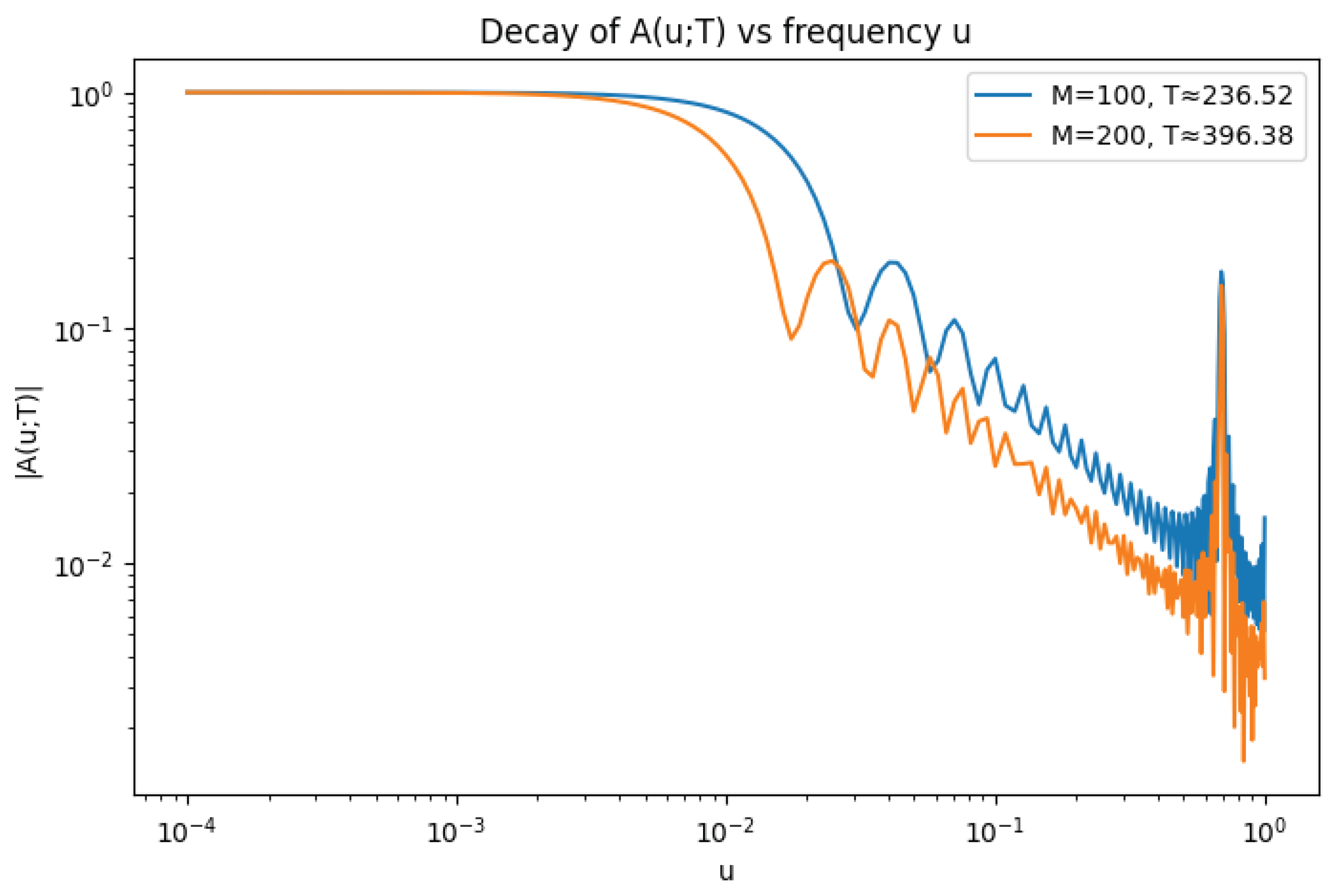
Table 2.
Numerical estimates of pair-correlation decay constants. Here M is the number of zeros used, T the height of the largest zero, , and the fitted exponent from .
Table 2.
Numerical estimates of pair-correlation decay constants. Here M is the number of zeros used, T the height of the largest zero, , and the fitted exponent from .
| M | T | N | ||||
|---|---|---|---|---|---|---|
| 100 | 236.52 | 100 | 0.6 | 0.361 | 0.173 | 1.032 |
| 100 | 236.52 | 100 | 0.8 | 0.257 | 0.173 | 1.032 |
| 100 | 236.52 | 100 | 1.0 | 0.183 | 0.173 | 1.032 |
| 200 | 396.38 | 200 | 0.6 | 0.342 | 0.151 | 1.057 |
| 200 | 396.38 | 200 | 0.8 | 0.239 | 0.151 | 1.057 |
| 200 | 396.38 | 200 | 1.0 | 0.167 | 0.151 | 1.057 |
Table 3.
Summary of tunable parameters in the entropy–sieve method.
| Param. | Role | Typical choice | Trade-off |
|---|---|---|---|
| Truncation length | –8 (polylog) | Larger A: smaller remainder, harder moments | |
| Approx. failure set | Bigger B ⇒ bigger A | ||
| Low-entropy set | Block length | Larger m: better entropy, costlier cumulants | |
| C | Remainder tolerance | –3 | Larger C: stronger control, bigger A |
| B | Power-saving exponent | –10 | Larger B: bigger A or higher moments |
| Small-gap sieve rate | –2 | Larger : faster decay, limited by MGF | |
| MGF tail rate | , | Fixed by X, controls linear tail | |
| m | Entropy block length | slowly | Larger m: smaller entropy set, more cost |
Disclaimer/Publisher’s Note: The statements, opinions and data contained in all publications are solely those of the individual author(s) and contributor(s) and not of MDPI and/or the editor(s). MDPI and/or the editor(s) disclaim responsibility for any injury to people or property resulting from any ideas, methods, instructions or products referred to in the content. |
© 2025 by the authors. Licensee MDPI, Basel, Switzerland. This article is an open access article distributed under the terms and conditions of the Creative Commons Attribution (CC BY) license (http://creativecommons.org/licenses/by/4.0/).
Copyright: This open access article is published under a Creative Commons CC BY 4.0 license, which permit the free download, distribution, and reuse, provided that the author and preprint are cited in any reuse.


