
Submitted:
02 September 2025
Posted:
03 September 2025
You are already at the latest version
Abstract
Objective: Stress recognition is a widely investigated and debated area in biomedical research. Physiological monitoring has gained increasing attention as one of the methodologies used to assess an individual's stress level. In this study, we investigated the effectiveness of a novel normalization technique applied to multi-domain physiological data for the objective classification of stress levels using a feature extraction approach. Methods: Electrocardiographic (ECG) and respiratory data from a publicly available database, collected from drivers experiencing various stress levels, underwent a novel inter-subject normalization procedure. This method involved adjusting the time scale of the original data to a common scale across subjects according to fixed resting heart and respiratory rates. Subsequently, a feature-based stress state classification procedure was conducted using the Support Vector Machine (SVM) algorithm. The efficacy of this inter-subject normalization procedure was assessed by comparing the classification results obtained using features from the original signals with those obtained from the inter-subject normalized signals. Additionally, the inter-subject normalization procedure was compared with two common feature normalization approaches: standardization and scaling. Results: Features derived from the subject-normalized signals yielded improved performance, significantly enhancing accuracy from 68% to 73% as well as precision and sensitivity. Conclusion: The novel inter-subject normalization procedure proves to be an effective technique for highlighting differences in features among various stress states and for mitigating basal physiological variability across subjects. Significance: Using inter-subject normalization on multi-domain physiological signals holds promise as a method to improve multilevel stress classification through feature extraction, ensuring that the features maintain their correspondence even after the normalization process.
Keywords:
driving stress
; classification
; Support Vector Machine (SVM)
; electrocardiogram
; breath
; data normalization
; stress classification
; machine learning
; imbalanced data
1. Introduction
Stress is a physiological response to various factors arising in individuals unable to consciously handle a specific situation. During a stressful situation, the sympathetic nervous system (SNS) is responsible for the fight-or-flight physiological reaction of the body, resulting in vasoconstriction, increased blood pressure and heart rate [1]. In the long term, stress can lead to different health problems, being directly related to several physiological processes such as those involving the autonomic nervous system [2], the immune systems [3], and the cardiovascular and respiratory systems [4].
Stress has been deeply investigated in recent years [1,5], given the relevant consequences of a prolonged stressful condition on the body. Nevertheless, the detection of stress remains a challenging task, since no standardized and validated methodology for stress assessment has been established as the gold standard. Among the methods used to measure stress, there are questionnaires [6,7], the visual analogue scale [8], and the detection of specific biomarkers (e.g., cortisol) related to the stress level [9,10]. Scale-related stress assessment methods do not require expensive tools but are time-consuming and non-objective. On the contrary, stress evaluation methods based on biomarkers give more objective results, but they require invasive and sophisticated tools. In addition, a continuous monitoring is very difficult to be carried out, either employing questionnaires or biomarker methodologies.
Given the drawbacks of the above-indicated detection methods, stress assessment through wearable sensors capable of acquiring physiological signals has emerged as a highly promising approach in recent times. Wearable devices are now even smaller in size and more affordable [11], thus becoming non-intrusive tools able to handle continuous monitoring. Furthermore, the recent growth of classification and machine learning algorithms in the physiological data analysis area has profoundly ameliorated stress evaluation [12,13]. In this context, the most employed biosignals are the electrocardiographic (ECG) [14,15], electromyographic (EMG) [16], electroencephalographic (EEG) [17], and photoplethysmographic (PPG) [18] signals [19]. These signals are often combined in a multi-domain approach which takes into account the interaction between multiple physiological data to better analyze the dynamics of each signal and extract further useful information.
Starting from the acquired biosignals, several methods have been reported in the literature to determine the stress level of a subject [12,19], mostly based on the extraction of various features from the signals, followed by a classifier to predict the stress level. For example, Gupta and colleagues [20] employed a support vector machine (SVM) classification on features extracted from the EEG signal. This classificatory approach was also used in [21] with the combination of ECG and EMG signals, obtaining an excellent binary classification accuracy. Other studies used the K-Nearest Neighbors (KNN) algorithm for classification using either ECG [15] or EEG [17] signals.
Although most machine learning approaches can predict the stress level of a subject with good accuracy, they do not consider a critical aspect related to physiological data, i.e., the inter-subject variability. Physiological signals, whether acquired at rest or in response to stimuli, exhibit significant subject-dependency. For example, a normal resting heart rate can vary considerably, typically ranging from 60 to 100 beats per minute [22]. Furthermore, other critical subject-specific physiological features can depend on respiratory or electrodermal activity signals [23]. In this context, some studies aiming to detect stress have employed either feature extraction or deep learning approaches, often incorporating amplitude normalization to account for inter-subject amplitude differences. However, time-related differences among subjects are often not adequately addressed. Common normalization techniques like scaling [24], and feature standardization [25] do not account for individual subject dependencies in the time domain, particularly concerning raw signals.
One possible approach to overcome this limitation is to normalize features by transforming the original feature vector into a common feature space where the feature exhibits the same mean or an arbitrary value across all subjects. However, this approach has a limitation: normalization is applied to a single feature independently (e.g., the RR interval), leading to a loss of correspondence with other features derived from the same signal. For instance, in the case of normalized RR features [26,27], the RR series is normalized by the mean value of all RR intervals within one ECG recording. Yet, the remaining extracted features are often derived from the original, unnormalized signal, thereby losing their association with the normalized RR feature.
Therefore, it is crucial to develop a normalization procedure that addresses this limitation. Such a procedure should enable the extraction of all features from a signal already in a normalized domain, ensuring that all features remain interconnected and associated within the same normalized framework.
In this context, Gasparini et al. [28] introduced a methodology for classifying PPG signal features that included an inter-subject normalization procedure to mitigate variability between individuals. Their approach first determines each subject’s resting heart rate, then uses resampling to map the data into a new domain where all subjects share a uniform resting heart rate.
In this work, we propose a new interpretation of this inter-subject normalization algorithm, specifically tailored for multi-domain feature extraction in the context of multilevel stress classification. We validated our approach using an open-access database of multimodal physiological data collected during various driving conditions [29]. A key distinction from Gasparini et al.’s method is that we applied the inter-subject normalization procedure to two physiological signals: ECG and respiratory data. Notably, our novel methodology operates directly on the raw physiological signals, transforming them into a different domain. This means that any features subsequently extracted from these normalized signals are inherently normalized within a common framework. The structure of this normalization is directly determined by the specific features used in the normalization process itself—heart rate for ECG signals and breath rate for respiratory signals in this project. This ensures a strong and inherent interrelation among all extracted features.
The performance of this algorithm was tested in a feature-based classification of driving stress using an SVM classifier. The features, derived from various physiological signals, were combined during the classification step. The classification performances were then compared when either skipping or utilizing this inter-subject normalization procedure in the preprocessing step. Additionally, these results were compared with those obtained using other commonly employed feature normalization approaches.
2. Materials and Methods
2.1. Physiological Data
The data used in this study belongs to the database of J.A. Healey and colleagues [29], composed of multimodal synchronized physiological data and video recorded on 16 subjects in different driving conditions.
Three different stress states were elicited during the experimental session, each one associated with a specific driving condition: low stress (resting, no driving), high stress (city driving) and medium stress (highway driving). The low-stress state was collected on two 15 minutes sessions respectively at the beginning and at the end of the experiment (herein referred as resting1 and resting2). In this condition, the subjects were sitting in a garage with their eyes closed, while the car was parked and idle. The medium-stress state was monitored while driving on the highway in two sessions (highway1 and highway2). The high stress was induced by driving in the congested streets of Boston (three driving phases named city1, city2 and city3). Depending on the traffic, acquisitions lasted from 50 to 90 min including the resting state.
The signals taken into account in this study were the ECG waveform, acquired through lead II configuration (sampling frequency of 496 Hz), and the respiration signal recorded through an elastic Hall effect sensor monitoring the chest cavity expansion (acquired at 31 Hz). Only subjects who had both ECG and respiratory data available for each stress state were considered, thereby excluding six subjects from the analysis.
2.2. Signal Preprocessing
The data preprocessing procedure prepared the raw physiological data for the successive feature extraction step. Following previous works [30], the preprocessing in this study consisted in filtering the raw physiological data and then partitioning the data based on the labelled stress state.
The raw ECG signal was filtered using a zero-phase passband Butterworth filter (0.1-115 Hz cutoff frequencies). For the raw respiratory signal, its relative mean value was first removed, and then the signal was filtered with a zero-phase bandpass Butterworth filter (0.01-5 Hz cutoff frequencies). Both the ECG and the respiratory signals were then resampled to 250 Hz, ensuring high data quality and reducing computational processing. The filtered signals were subsequently organized into a structure containing the three primary stress phases based on the reported labels: resting, highway driving, and city driving.
Subsequently, each signal was segmented into 20-second windows with a 5-second overlap, thus performing a data augmentation, as this increased the number of samples available for classification. The choice of a 20-second window length was made to maximize the number of windows while preserving temporal information within each window [31,32,33]. The 5-second overlap was chosen to ensure independence between samples, which, in turn, enhances the model’s ability to generalize during stress state prediction. According to the study by Farias da Silva and colleagues [34], a 5-second overlap was found to be the best compromise for the overlapping window data augmentation technique.
In the following analyses, two different sets of data originating from the same database were utilized to emphasize the effects of the inter-subject normalization procedure. The first dataset comprised raw signals subjected to the preprocessing procedure without any additional modifications, as described in this paragraph. The second dataset was generated by applying the inter-subject normalization process before the feature extraction step. Specifically, for each driver, the resting phases were considered for subject normalization. From now on, the term original signal will be used to identify the first dataset, while the second dataset will be identified by the term subject-normalized signal.
All the procedures, including the preprocessing steps, were conducted in the MATLAB environment, version 2022b [35].
2.3. Inter-Subject Normalization
This study employs an inter-subject normalization algorithm to account for inherent physiological variability among individuals during stress classification. During resting states, characterized by low stress, each driver exhibits unique physiological characteristics. For instance, a healthy individual’s resting heart rate typically ranges from 60 to 100 beats per minute (bpm), while their respiratory rate can vary from 12 to 20 breaths per minute [22,36]. This physiological diversity persists across all stress levels and can significantly impact classification accuracy.
Consider an example: a heart rate of 80 bpm might be recorded for one subject during rest, but the same heart rate could indicate moderate stress in another subject. This observation extends to other physiological conditions and stress levels. Without addressing this inter-subject variability, classification algorithms trained and tested with inconsistent data can lead to misclassification errors.
To mitigate this issue, this paper presents a novel resampling procedure applied to raw ECG and respiratory signals. This approach extends previous work by Gasparini and colleagues [28], offering a multidomain solution. The primary goal of this procedure is to reduce inter-subject variability in specific physiological features during the resting state. This reduction improves the ability to first identify changes in these features across different stress levels and, indirectly, extends the normalization to all other features extracted from the signals, as the signals themselves are transformed into a new normalized domain.
The normalization procedure involves selecting a specific feature from each physiological signal (ECG and respiration) to serve as the basis for normalization. Subsequently, a new sampling frequency is assigned to the original signal. This adjustment ensures consistency of the selected feature among all subjects within the resting phase. The inter-subject normalization procedure for both ECG and breath signals is further detailed in the following subsections.
2.3.1. ECG Signal
The inter-subject normalization procedure on the ECG signal was conducted considering the heart rate as the normalized feature. This ensured that, after normalization, all subjects exhibited the same average heart rate during the resting state.
Starting from the raw ECG signal with a sampling frequency equal to 250 Hz, the Pan-Tompkins algorithm [37] was applied to detect the R peaks during the two resting phases. Subsequently, the R-R interval (RRI) time series were extracted (Figure 1a), from which the heart rate series was derived as the inverse of the RRI time series. The mean heart rate across the two resting phases was then calculated as a reference value using the following equation:
where is the time (expressed in milliseconds) corresponding to the R peak, and N and M represent the number of R-peaks detected in the first and second resting phases, respectively.
The inter-subject normalization procedure aimed to transform all subjects’ data into a subject-normalized domain. In this domain, each subject’s resting heart rate was standardized to a predefined value , which was set to 70 beats per minute (bpm). This normalization was achieved by resampling the raw ECG signals at a new sampling frequency , which varied across subjects. The determination of was based on the ratio between the chosen resting frequency and each subject’s mean resting heart rate , as follows:
where is the original sampling frequency (250 Hz). The resampling frequency determined from the resting phase heart rate, was then consistently applied to the ECG signals recorded during other stress phases (highway driving and city driving). This crucial step ensured that the temporal relationships and feature characteristics across different stress states were preserved following normalization.
Each subject could potentially exhibit a different heart rate during resting conditions. Therefore, following the described inter-subject normalization procedure, the raw ECG of each subject was resampled into a new domain characterized by a resampling frequency value determined by the ratio as described in (2). As an example, given a device that acquired the ECG signal with an original sampling frequency equal to 250 Hz:
- If a driver exhibited a heart rate higher than 70 bpm at rest in the original signal, the value of the new resampling frequency was lower than 250 Hz.
- If the driver presented a heart rate lower than 70 bpm at rest, the value of the new resampling frequency was higher than 250 Hz.
The inter-subject normalization procedure had two main consequences. Firstly, it shifted the signals of each subject into a new common domain based on chosen specific features (heart rate during resting in the case of ECG). In this new domain, each subject exhibited the same average value of the considered feature, maintaining unaffected the relative intra-subject difference during both resting and stressful conditions. Furthermore, the length of the resampled signals was different than the original ones (Figure 1b). This was caused by the resampling procedure introducing a lengthening or shortening of the signal due to the decreasing or increasing of the resampling frequency, respectively.
2.3.2. Respiratory Signal
Analogous to the procedure carried out on the ECG signal, the inter-subject normalization procedure aimed to resample the original respiratory signal. This was done with a new frequency to ensure all subjects exhibited the same breath rate during the resting state. Therefore, the breath rate feature was chosen as the reference. Specifically, the resampling frequency , defined by the following equation, was employed:
Here, is the selected resting breathing frequency (in this project, set to 14 breaths per minute). The value of indicates the mean breath frequency during the two resting periods detected on the original signal and derived as the inverse of the breath-to-breath interval (BBI) series. To obtain this value, the inspiration peak positions were first determined on the original signal (Figure 1c). Subsequently, the time differences between consecutive peaks were calculated. These peak-to-peak series, when multiplied by 60 and divided by a factor of 1000, indicate the breath rate values expressed in breaths per minute. The final value was obtained by averaging all the breath rate values within the two resting phases. The value of derived in Equation 3 was then used to resample the respiratory signal across all stress phases, thereby preserving the temporal relationship between stress states for each considered feature.
Given that the original sampling frequency was consistent across different drivers, variations in the obtained resampling frequency across drivers were solely determined by the ratio between and . Consequently, a breath rate on the original signal higher than 14 breaths per minute resulted in a resampling frequency lower than 250 Hz. Conversely, the resampling frequency was higher than 250 Hz. The same implications of the inter-subject normalization outlined in the previous paragraph for the ECG traces also apply to the respiratory signals.
2.4. Feature Extraction
Feature extraction was performed on 20-second windows of the signal. This methodology required the exclusive use of time-domain features, as a 20-second duration was considered inadequate for a comprehensive frequency-domain analysis. Accurate frequency-domain analysis typically requires signals of greater length and a higher density of data points to yield statistically significant results [38,39]. By segmenting the original signal into shorter windows, the number of resultant feature vectors available for the subsequent classification step was augmented, thereby contributing to a more generalizable algorithm. The 20-second window length was specifically chosen to balance the need for sufficient temporal information with the necessity to generate a substantial number of samples.
In the context of feature extraction in the time domain, it was essential to accurately identify key morphological points of interest in each signal. For instance, in the ECG signal, the identification of R peaks was crucial, while in the respiratory signal, the focus was on detecting respiratory peaks.
In this study, we employed a modified version of the Pan-Tompkins algorithm [40] to detect the positions of R peaks in the ECG signal from each window, resulting in the creation of the RR interval time series. From this, the obtained time-domain features were the average RR interval (), the standard deviation () and the root mean square of successive RR interval differences () [41]. In addition, the standard deviation of successive RR interval differences (), the number of R peaks in each window that differ more than 50 milliseconds () and the associated percentage () were calculated [42].
To extract the time-domain indices of the respiratory signal, the maximum and minimum points within each window were identified. The time difference between each maximum point was considered as a respiratory act. Therefore, the respiratory rate () was determined by calculating the average of the inverse of the time distances between the maxima. Inspiration and expiration times were investigated by computing the average rise time () and fall time () of the breathing signal within each respiratory act. Additionally, the average inspiration and expiration areas were extracted by considering the area under the inspiration and expiration phases in the respiratory signal, respectively.
It is worth noting that the difference in the length of raw signals and those subjected to the inter-subject normalization did not result in a difference in the length of the time series used in the feature extraction phase, for both the RRI and the BBI series. Additionally, any potential changes introduced by the inter-subject normalization process, particularly those associated with discrepancies in the time length between ECG signal samples and respiratory signal samples, did not affect stress classification. This is because the features were independently extracted from each physiological signal.
2.5. Data Organization and Imbalance Class Management
The feature dataset was organized in a table where each row represented a 20-s window, and each column corresponded to a specific feature. In total, 12 features were extracted from each of the 2979 windows for the original signals and each of the 2974 windows for the normalized signals. This slight difference in the number of samples was due to variations in the length of the normalized signals. These length changes resulted from different resampling frequencies applied to each subject, which in turn led to a different number of 20-second windows being obtainable from the complete signals.
An analysis of the number of windows associated with each stress label revealed a clear imbalance in class distribution. Specifically, for the time series derived from the original signals:
- The resting condition had 1132 samples.
- The city driving condition had 1275 samples.
- The highway driving condition had 572 samples.
A similar sample distribution across the different classes was observed for the normalized signals. To address this class imbalance during classification and mitigate potential bias and inaccuracy that can arise when training a machine learning model on imbalanced data, the Synthetic Minority Oversampling Technique (SMOTE) [43] was employed. This algorithm generates synthetic samples for classes with fewer existing samples by interpolating between points in the feature space. Applying SMOTE ensured an equal representation of samples across all classes.
2.6. Stress State Classification
To compare our findings with prior research on the same dataset, we employed a Support Vector Machine (SVM) for classification, mirroring the methodology of a previous study [30]. Specifically, we utilized a Gaussian SVM, characterized by its Gaussian kernel function, a common choice for classification tasks [44,45]. The SVM was trained on 80% of the dataset, with the remaining 20% reserved for testing. This random partitioning strategy was employed to mitigate overfitting and ensure an unbiased evaluation of the model’s ability to generalize and accurately predict stress in unseen data.
Additionally, to account for potential variations in model performance due to different training and testing splits, we repeated the training and testing phases 100 times. This repetition minimizes the stochastic behavior of the process, and the final classification performances were obtained by averaging the values across these 100 iterations.
For each set of results, a global confusion matrix was generated. This matrix illustrates the relationship between predicted and true labels, from which key performance metrics—including accuracy, sensitivity, specificity, precision, and F-measure—were derived to comprehensively evaluate the model’s performance.
3. Inter-Subject Normalization Validation
The inter-subject normalization procedure was evaluated by comparing features extracted from subject-normalized signals with those from original signals. This evaluation also included comparisons to features processed using two common machine learning normalization techniques: standardization [46] and scaling [24].
Standardization
In the standardization procedure, each feature—where a single element in a row represented a feature derived from a 20-second window of the original signal—was normalized as follows:
Here, indicates the original feature array, the mean of , and the standard deviation of . This normalization resulted in a feature array with an average value equal to zero and a standard deviation equal to one.
Scaling
The scaling procedure remapped all features to the same scale, ensuring comparable ranges across features and subjects. For a single feature, the scaling procedure was represented as:
Here, is the original features array and indicates the array with the considered features rescaled to the range [0, 1].
Inter-Subject Normalization
Unlike standardization and scaling, which directly operated on the features, inter-subject normalization modified the original signal. Consequently, features derived from inter-subject normalized signals retained their original relationships. In contrast, standardization and scaling procedures acted independently on each feature, potentially leading to a loss of inter-feature information.
To evaluate the performance of each normalization procedure, the Chi-square goodness-of-fit test was applied to assess the normality of the distributions of performance metrics (i.e., precision, sensitivity, and accuracy). These metrics were obtained from 100 iterations of training and testing an SVM model. The original data served as the baseline for comparison. Specifically, the test was conducted on performance distributions derived from the original features, comparing them with distributions from subject-normalized features, standardized features, and scaled features.
To ensure a robust statistical comparison among the four groups, the ANOVA test was employed. Additionally, the Bonferroni method was applied to account for multiple comparisons in the statistical analysis. A two-sample parametric unpaired Student’s t-test was performed to detect significant differences between groups. This test specifically aimed to compare the performances achieved using the three different normalization procedures with the performances derived from the original data. The null hypothesis for all conditions was that there were no significant differences between the original features and the features obtained after inter-subject normalization, standardization, or scaling procedures.
4. Results
Following the inter-subject normalization procedure, both the electrocardiogram (ECG) and respiratory signals were resampled to a new domain. This resampling was performed using the individual’s resting heart rate (HR) and resting respiratory rate (RR) as normalization features, respectively. Table 1 details the heart rates from the original signals and their associated resampling frequencies for each subject, while Table 2 provides the same information for breath rates. It’s important to note that a heart rate exceeding 70 bpm (or a breath rate greater than 14 breaths per minute) resulted in a resampling frequency lower than 250 Hz, and vice versa. This adaptive resampling ensured that the signals were transformed to a common domain relevant to each subject’s physiological baseline.
Starting from the inter-subject normalized signals, and following the feature extraction and classification procedures, the developed Support Vector Machine (SVM) model was rigorously assessed. A confusion matrix was generated for each of the four experimental conditions examined in this study:
- Original signals
- Subject-normalized signals
- Feature transformations through standardization
- Feature transformations using scaling procedures
An example of a confusion matrix for a single iteration is illustrated in Figure 2. This matrix was derived by training the SVM model on the training dataset and subsequently testing it on the unseen test data.
The performance metrics, averaged across 100 iterations for all four conditions, are presented in Table 3 in terms of mean and standard deviation. Accuracy results are also visually represented in Figure 3. In these figures, ‘n.s.’ as a superscript denotes no statistical significance, while three asterisks (∗∗∗) indicate statistical significance (p < 0.001) when comparing the original data to the considered group.
Our analysis revealed several key findings regarding the impact of different preprocessing techniques on model performance. When using the original, unprocessed data, the model consistently achieved precision, sensitivity, and accuracy of 68%, with specificity around 84%. On the other hand, both standardization and scaling procedures yielded very similar results to the original data, showing no substantial changes in precision, sensitivity, specificity, or accuracy. This suggests that these linear transformations alone did not significantly enhance the model’s ability to discriminate between classes in this context. In contrast, inter-subject normalization demonstrated an improvement in model performance. Precision, sensitivity, and accuracy all increased to 73%, while specificity also showed a slight improvement, reaching 86%. The superior statistical significance observed with subject-normalized data, as indicated by the three asterisks in Figure 3, further underscores the effectiveness of this method. These improvements strongly suggest that inter-subject normalization holds significant promise for enhancing the overall performance of the model in similar physiological signal analysis tasks.
5. Discussion
This study investigated the impact of inter-subject normalization on electrocardiographic (ECG) and respiratory signals to reduce physiological variability during stress state classification. We selected ECG and respiratory data due to their established relevance in stress research, as evidenced by previous studies [30,32,47]. These signals provide valuable insights into an individual’s physiological response to stress.
We performed a feature-based multilevel stress classification using a Support Vector Machine (SVM) classifier. This classification was conducted after applying inter-subject normalization and two widely used normalization procedures: standardization and scaling. Subsequently, we compared the classification performances derived from these procedures with those obtained from the original, unnormalized data.
When using the original ECG and respiratory signals, our classification model consistently achieved a precision, sensitivity, and accuracy of 68%, while specificity was approximately 84%. Applying standardization and scaling techniques yielded comparable performance values (Table 3), suggesting these methods do not significantly alter the model’s performance compared to using raw data. This outcome aligns with expectations, as both standardization and scaling primarily adjust data distribution without introducing substantial changes to the underlying information.
The inter-subject normalization procedure successfully reduced inter-subject variability in physiological features during the resting state, effectively aligning subjects to a common physiological domain. This normalization enhances the classification of stress levels by ensuring consistency in physiological data across resting and stressful conditions for different subjects. The results clearly demonstrated the effectiveness of this approach, showing significant improvements over the original data, standardization, and scaling procedures. Precision, sensitivity, and accuracy increased from 68% to 73%, and specificity improved by approximately two percentage points. The enhancement in precision and sensitivity is particularly noteworthy, as these metrics directly reflect the model’s ability to accurately identify instances of stress.
The inter-subject normalization procedure operates directly on the original signals, placing them in a transformed space defined by a distinct sampling frequency. This novel procedure ensures that each feature derived from the inter-subject normalized signals is already indirectly normalized. Crucially, this normalization structure depends solely on the specific features used in the normalization process (e.g., heart rate for ECG and breath rate for respiratory signals in this study). Consequently, each extracted feature becomes strongly interconnected with every other feature. In contrast, traditional feature normalization approaches like standardization and scaling independently modify each feature obtained from the original signal. These methods treat each feature in isolation, which can lead to a loss of consistency between features and varying levels of normalization, ultimately impacting the subsequent classification step. Our novel approach, by directly acting on the original signals and maintaining these crucial interconnections, offers a more robust framework for feature analysis in stress classification. This goes beyond simple, isolated feature normalization, such as only shifting a heart rate baseline to a specific value like 70 bpm, where other extracted features remain uncorrelated and the natural, intrinsic relationships between them are disrupted.
A critical aspect of implementing this technique is identifying the most appropriate feature for defining the inter-subject normalization rescaling. In this project, we distinctly used the mean heart rate and mean breath rate during resting phases for ECG and respiratory signals, respectively, given their distinct physiological meanings.
Other studies have utilized physiological signals for stress assessment with various experimental protocols. For example, Smets and colleagues [29] achieved approximately 82% classification accuracy using an SVM in a binary stress classification problem by combining ECG and respiratory features. Similarly, Han et al. [43] discriminated between three stress states with 84% accuracy using ECG and respiratory features. These studies often incorporated both time and frequency domain features, necessitating longer signal windows for adequate frequency resolution. In contrast, our proposed work effectively utilizes 20-second segments and the inter-subject normalization procedure to achieve efficient classification with strong performance, even without considering frequency domain features. This suggests the presented framework could potentially be employed for real-time stress classification based on ultra-short-term recordings.
However, further investigations are needed to thoroughly understand the effect of inter-subject normalization on the frequency domain and to explore the potential contribution of frequency-domain features in the stress classification step. Additionally, while the framework shows promise for short recordings, considering longer time windows for analysis would be beneficial for comprehensive understanding. It might also be useful to investigate the incorporation of additional physiological data suitable for the inter-subject normalization approach, such as electrodermal activity (EDA), electromyography (EMG), or advanced features from other wearable devices like accelerometers and skin temperature sensors. Combining various data types has the potential to enhance stress classification accuracy and offer a more comprehensive understanding of an individual’s stress response [19,29,32,48].
6. Conclusions
This study investigated the impact of a subject-normalization procedure on stress classification. It utilized ECG and respiratory physiological signals from 10 drivers across varying stress levels, employing a feature-driven methodology.
The findings demonstrate that this novel normalization procedure significantly improves stress classification compared to traditional standardization and scaling methods. The inter-subject normalization approach effectively reduced variability between individuals, leading to consistent results in both resting and stressful states. This enhancement was reflected in improved precision, sensitivity, and accuracy, indicating a greater ability to correctly identify stress. A key advantage of inter-subject normalization is its direct operation on the original signals, fostering strong interconnectivity among features. This differs from other methods that modify features independently. This novel procedure therefore establishes a deeper link between features, as they originate from a shared signal domain.
Future research should explore incorporating additional physiological data, extracting advanced features from wearable devices, and analyzing frequency-domain features. Such efforts could further enhance stress classification accuracy and provide a more complete understanding of stress responses. Given these results, this innovative inter-subject normalization technique shows strong potential for real-time stress classification in diverse applications like healthcare and stress management.
Funding
D.F. is founded by the European Union NextGenerationEU, iNEST project - Bandi Young Researchers - in the framework of the iNEST - Intercon-nected Nord-Est Innovation Ecosystem (iNEST ECS00000043 – CUP E63C22001030007). Views and opinions expressed are however those of the author(s) only and do not necessarily reflect those of the European Union or The European Research Executive Agency. Neither the European Union nor the granting authority can be held responsible for them. L.F. was supported by Italian Ministry of University and Research SiciliAn MicronanOTecH Research And Innovation CEnter “SAMOTHRACE” (MUR, PNRR-M4C2, ECS_00000022), spoke 3—Università degli Studi di Palermo “S2-COMMs—Micro and Nanotechnologies for Smart & Sustainable Communities” And DARE – DigitAl lifelong pRevEntion project (MUR, PNC, PNC0000002). R.P. is partially supported by the European Social Fund (ESF) Complementary Operational Programme (POC) 2014/2020 of the Sicily Region.
Conflicts of Interest
This statement accompanies the article “A Signal Normalization approach for Robust Driving Stress Assessment Using Multi-Domain physiological data” authored by Damiano Fruet and co-authored by Chiara Barà, Riccardo Pernice, Marta Iovino, Luca Faes and Giandomenico Nollo. Authors collectively affirm that this manuscript represents original work that has not been published and is not being considered for publication elsewhere. We also affirm that all authors listed contributed significantly to the project and manuscript. Furthermore, we confirm that none of our authors have disclosures, and we declare no conflict of interest.
References
- J. Taelman, S. Vandeput, A. Spaepen, and S. Van Huffel, “Influence of mental stress on heart rate and heart rate variability,” IFMBE Proc., vol. 22, pp. 1366–1369, 2008. [CrossRef]
- B. S. McEwen and P. J. Gianaros, “Stress and Allostasis Induced Brain Plasticity,” Annu. Rev. Med., vol. 62, no. 1, pp. 431–445, 2011. [CrossRef]
- J. J. Strain, “The psychobiology of stress, depression, adjustment disorders and resilience,” World J. Biol. Psychiatry, vol. 19, no. sup1, pp. S14–S20, 2018. [CrossRef]
- B. S. McEwen, “Mood disorders and allostatic load,” Biol. Psychiatry, vol. 54, no. 3, pp. 200–207, 2003. [CrossRef]
- S. Rabbani and N. Khan, “Contrastive Self-Supervised Learning for Stress Detection from ECG Data,” Bioengineering, vol. 9, no. 8, p. 374, 2022. [CrossRef]
- J. M. Taylor, “Psychometric analysis of the ten-item perceived stress scale,” Psychol. Assess., vol. 27, no. 1, pp. 90–101, 2015. [CrossRef]
- S. Cohen, T. Kamarck, and R. Mermelstein, “A Global Measure of Perceived Stress,” J. Health Soc. Behav., vol. 24, no. 4, pp. 385–396, 1983.
- F.-X. Lesage, S. Berjot, and F. Deschamps, “Clinical stress assessment using a visual analogue scale,” Occup. Med., vol. 62, no. 8, pp. 600–605, 2012.
- N. Ali and U. M. Nater, “Salivary Alpha-Amylase as a Biomarker of Stress in Behavioral Medicine,” Int. J. Behav. Med., vol. 27, no. 3, pp. 337–342, 2020. [CrossRef]
- D. H. Hellhammer, S. Wüst, and B. M. Kudielka, “Salivary cortisol as a biomarker in stress research,” Psychoneuroendocrinology, vol. 34, no. 2, pp. 163–171, 2009. [CrossRef]
- S. Patel, H. Park, P. Bonato, L. Chan, and M. Rodgers, “A review of wearable sensors and systems with application in rehabilitation,” J. Neuroengineering Rehabil., pp. 1–17, 2012.
- M. Zanetti et al., “Assessment of mental stress through the analysis of physiological signals acquired from wearable devices,” Lect. Notes Electr. Eng., vol. 544, pp. 243–256, 2018. [CrossRef]
- N. Garau, D. Fruet, A. Luchetti, F. De Natale, and N. Conci, “A multimodal framework for the evaluation of patients’ weaknesses, supporting the design of customised AAL solutions,” Expert Syst. Appl., vol. 202, no. December 2021, p. 117172, 2022. [CrossRef]
- P. Karthikeyan, M. Murugappan, and S. Yaacob, “ECG signals based mental stress assessment using wavelet transform,” Proc. - 2011 IEEE Int. Conf. Control Syst. Comput. Eng. ICCSCE 2011, pp. 258–262, 2011. [CrossRef]
- S. Z. Bong, M. Murugappan, and S. Yaacob, “Analysis of electrocardiogram (ECG) signals for human emotional stress classification,” Commun. Comput. Inf. Sci., vol. 330 CCIS, no. September 2013, pp. 198–205, 2012. [CrossRef]
- S. Pourmohammadi and A. Maleki, “Stress detection using ECG and EMG signals: A comprehensive study,” Comput. Methods Programs Biomed., vol. 193, 2020. [CrossRef]
- T. Rahman, A. K. Ghosh, M. H. Shuvo, and M. Rahman, “Mental Stress Recognition using K-Nearest Neighbor ( KNN ) Classifier on EEG Signals,” Int. Conf. Mater. Electron. Inf. Eng. ICMEIE, no. June 2015, pp. 1–4, 2015.
- S. Heo, S. Kwon, and J. Lee, “Stress Detection with Single PPG Sensor by Orchestrating Multiple Denoising and Peak-Detecting Methods,” IEEE Access, vol. 9, pp. 47777–47785, 2021. [CrossRef]
- M. Zanetti et al., “Multilevel assessment of mental stress via network physiology paradigm using consumer wearable devices,” J. Ambient Intell. Humaniz. Comput., 2019. [CrossRef]
- R. Gupta, M. A. Alam, and P. Agarwal, “Modified Support Vector Machine for Detecting Stress Level Using EEG Signals,” Comput. Intell. Neurosci., vol. 2020, 2020. [CrossRef]
- K. Soman, A. Sathiya, and N. Suganthi, “Classification of stress of automobile drivers using Radial Basis Function Kernel Support Vector Machine,” 2014 Int. Conf. Inf. Commun. Embed. Syst. ICICES 2014, no. 978, pp. 4–8, 2015. [CrossRef]
- A. H. Association, “All About Heart Rate (Pulse).” [Online]. Available: https://www.heart.org/en/health-topics/high-blood-pressure/the-facts-about-high-blood-pressure/all-about-heart-rate-pulse.
- D. Wu et al., “Optimal arousal identification and classification for affective computing using physiological signals: Virtual reality stroop task,” IEEE Trans. Affect. Comput., vol. 1, no. 2, pp. 109–118, 2010. [CrossRef]
- J. A. Healey and R. W. Picard, “Detecting stress during real-world driving tasks using physiological sensors,” IEEE Trans. Intell. Transp. Syst., vol. 6, no. 2, pp. 156–166, 2005. [CrossRef]
- X. Cui et al., “On the variability of heart rate variability—evidence from prospective study of healthy young college students,” Entropy, vol. 22, no. 11, pp. 1–26, 2020. [CrossRef]
- C.-C. Lin and C.-M. Yang, “Heartbeat Classification Using Normalized RR Intervals and Morphological Features,” Math. Probl. Eng., vol. 2014, no. 1, p. 712474, Jan. 2014. [CrossRef]
- C. C. Lin and C. M. Yang, “Heartbeat Classification Using Normalized RR Intervals and Wavelet Features,” in 2014 International Symposium on Computer, Consumer and Control, Taichung, Taiwan: IEEE, June 2014, pp. 650–653. [CrossRef]
- F. Gasparini, A. Grossi, M. Giltri, and S. Bandini, “Personalized PPG Normalization Based on Subject Heartbeat in Resting State Condition,” Signals, vol. 3, no. 2, pp. 249–265, 2022. [CrossRef]
- J. A. Healey and R. W. Picard, “Detecting stress during real-world driving tasks using physiological sensors,” IEEE Trans. Intell. Transp. Syst., vol. 6, no. 2, pp. 156–166, 2005. [CrossRef]
- D. Fruet, C. Bara, R. Pernice, L. Faes, and G. Nollo, “Assessment Of Driving Stress Through SVM And KNN Classifiers On Multi-Domain Physiological Data,” MELECON 2022 - IEEE Mediterr. Electrotech. Conf. Proc., pp. 920–925, 2022. [CrossRef]
- J. Tervonen, K. Pettersson, and J. Mäntyjärvi, “Ultra-short window length and feature importance analysis for cognitive load detection from wearable sensors,” Electron. Switz., vol. 10, no. 5, pp. 1–19, 2021. [CrossRef]
- E. Smets et al., “Comparison of Machine Learning Techniques for Psychophysiological Stress Detection,” Pervasive Comput. Paradig. Ment. Health, pp. 13–22, 2016. [CrossRef]
- M. Gjoreski et al., “Datasets for cognitive load inference using wearable sensors and psychological traits,” Appl. Sci. Switz., vol. 10, no. 11, 2020. [CrossRef]
- M. A. Farias da Silva, R. L. De Carvalho, and T. da S. Almeida, “Evaluation of a Sliding Window mechanism as DataAugmentation over Emotion Detection on Speech,” Acad. J. Comput. Eng. Appl. Math., vol. 2, no. 1, pp. 11–18, 2021. [CrossRef]
- MathWorks, MatLab. (2022). [Online]. Available: https://it.mathworks.com.
- A. Addeh, F. Vega, P. R. Medi, R. J. Williams, G. B. Pike, and M. E. MacDonald, “Direct machine learning reconstruction of respiratory variation waveforms from resting state fMRI data in a pediatric population,” NeuroImage, vol. 269, no. October 2022, p. 119904, 2023. [CrossRef]
- G. Nollo, G. Speranza, R. Grasso, R. Bonamini, L. Mangiardi, and R. Antolini, “Spontaneous beat-to-beat variability of the ventricular repolarization duration,” J. Electrocardiol., vol. 25, no. 1, pp. 9–17, 1992. [CrossRef]
- F. Shaffer, S. Steven, and Z. Meehan, “The Promise of Ultra-Short-Term ( UST ) Heart Rate Variability Measurements,” Biofeedback, vol. 44, 2016. [CrossRef]
- G. Volpes et al., “Feasibility of Ultra-Short-Term Analysis of Heart Rate and Systolic Arterial Pressure Variability at Rest and during Stress via Time-Domain and Entropy-Based Measures,” Sensors, 2022.
- J. Pan and W. J. Tompkins, “A real-time QRS detection algorithm,” IEEE Trans. Biomed. Eng., no. 3, pp. 230–236, 1985.
- F. Shaffer and J. P. Ginsberg, “An overview of heart rate variability metrics and norms,” Front. Public Health, p. 258, 2017.
- F. Shaffer, Z. M. Meehan, and C. L. Zerr, “A Critical Review of Ultra-Short-Term Heart Rate Variability Norms Research,” Front. Neurosci., vol. 14, no. November, pp. 1–11, 2020. [CrossRef]
- N. V. Chawla, K. W. Bowyer, L. O. Hall, and W. P. Kegelmeyer, “SMOTE: Synthetic Minority Over-sampling Technique Nitesh,” J. Artif. Intell. Res., pp. 321–357, 2002. [CrossRef]
- P. Virdi, Y. Narayan, P. Kumari, and L. Mathew, “Discrete Wavelet Packet based Elbow Movement classification using Fine Gaussian SVM,” 1st IEEE Int. Conf. Power Electron. Intell. Control Energy Syst. ICPEICES 2016, pp. 1–5, 2017. [CrossRef]
- D. Fruet, “Affective state classification using timing-related features from short windowed PPG signal,” 2023 IEEE Int. Workshop Metrol. Ind. 40 IoT MetroInd40IoT, pp. 153–158, 2023. [CrossRef]
- Y. Zhang, S. Wei, L. Zhang, and C. Liu, “Comparing the Performance of Random Forest, SVM and Their Variants for ECG Quality Assessment Combined with Nonlinear Features,” J. Med. Biol. Eng., vol. 39, no. 3, pp. 381–392, 2019. [CrossRef]
- L. Han, Q. Zhang, X. Chen, Q. Zhan, T. Yang, and Z. Zhao, “Detecting work-related stress with a wearable device,” Comput. Ind., vol. 90, pp. 42–49, 2017. [CrossRef]
- M. Zanetti et al., “Information dynamics of the brain, cardiovascular and respiratory network during different levels of mental stress,” Entropy, vol. 21, no. 3, 2019. [CrossRef]
Figure 1.
Effect of the inter-subject normalization on the length of exemplary ECG and breathing signals. a) original 10-s window ECG signal containing 13 beats and b) 10-s window subject-normalized ECG signal containing 14 beats. c) original 50-swindow respiratory signal containing 12 breaths and d) 50-s window subject-normalized respiratory signal containing 11 breaths.
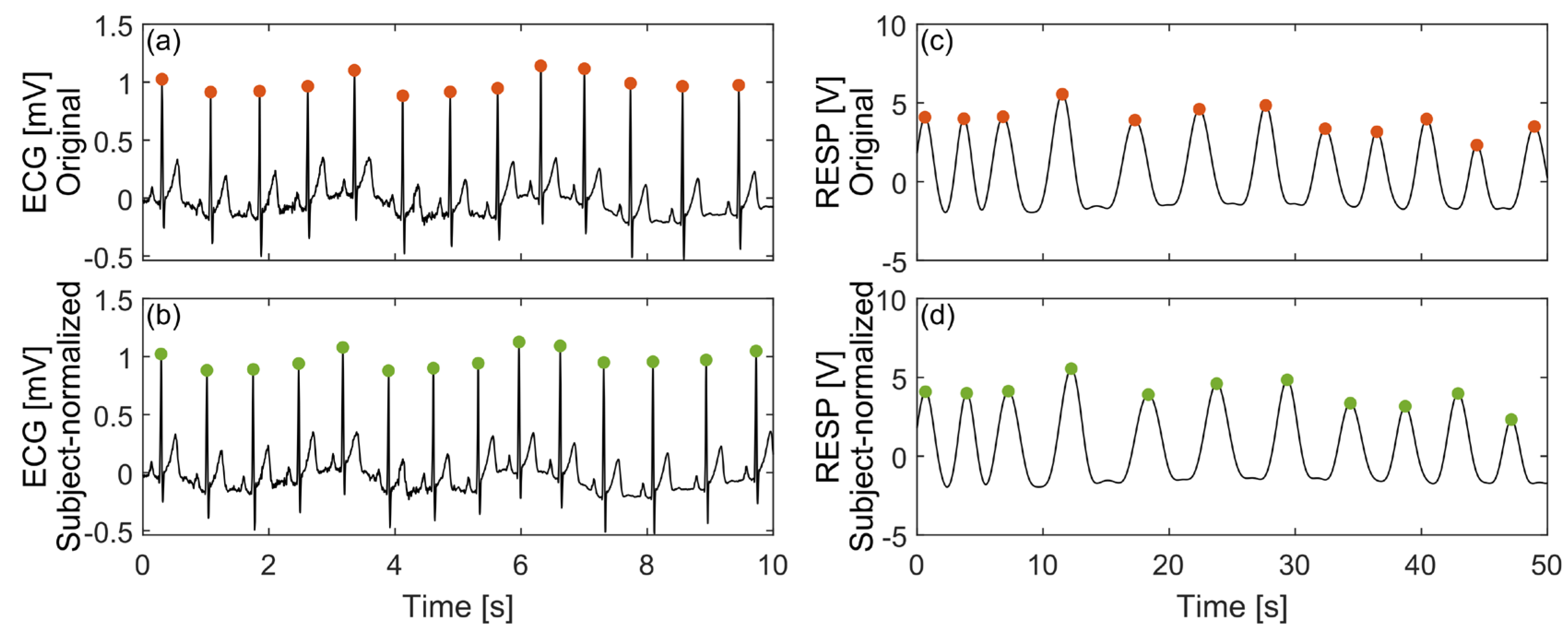
Figure 2.
Confusion matrix obtained by considering the original testing data in a single iteration.
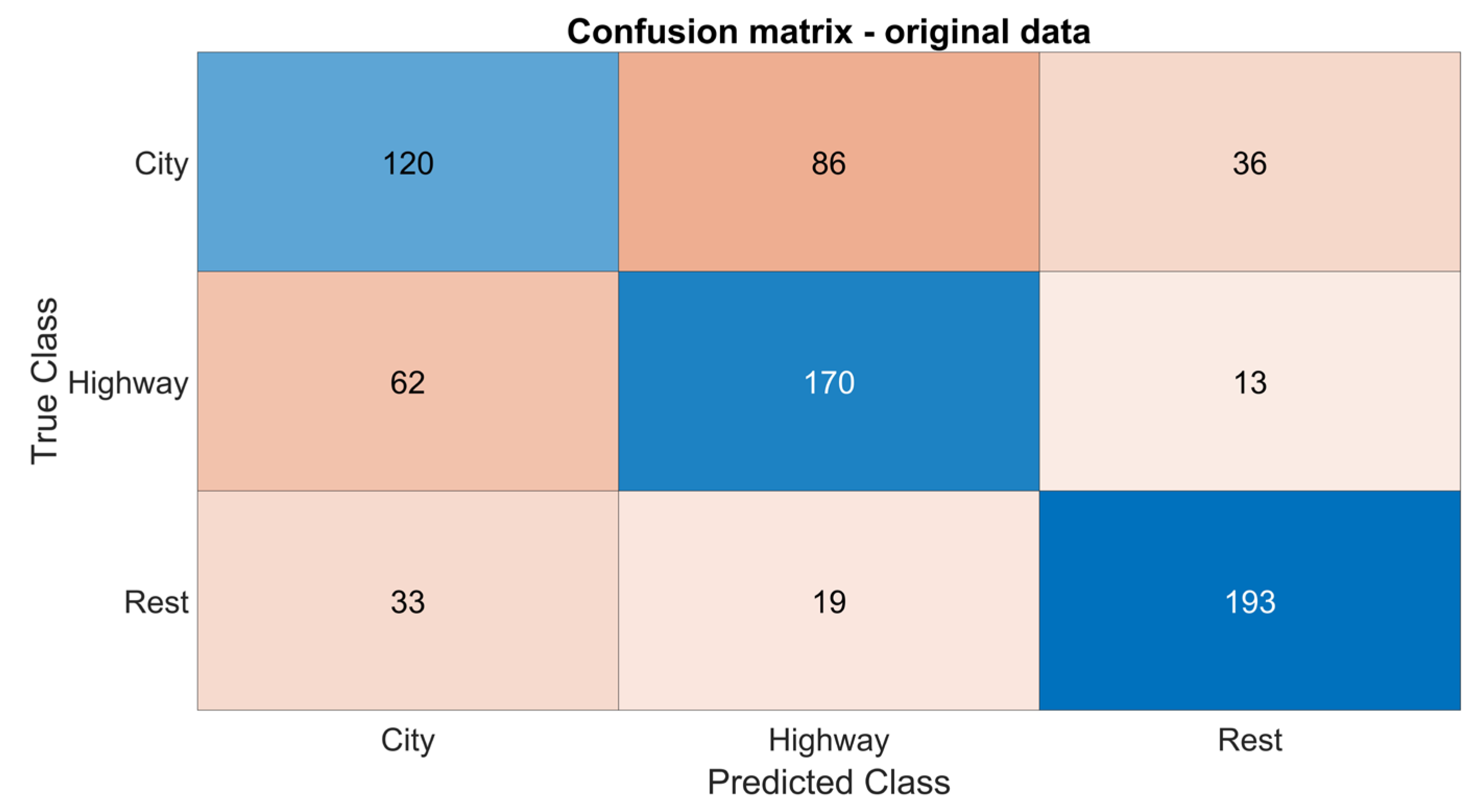
Figure 3.
Box plot and reported statistical significance obtained through a parametric Student’s t-test comparing model accuracy using features derived from original data, scaled features, standardized normalized features, and features obtained from inter-subject normalized signals.
Figure 3.
Box plot and reported statistical significance obtained through a parametric Student’s t-test comparing model accuracy using features derived from original data, scaled features, standardized normalized features, and features obtained from inter-subject normalized signals.
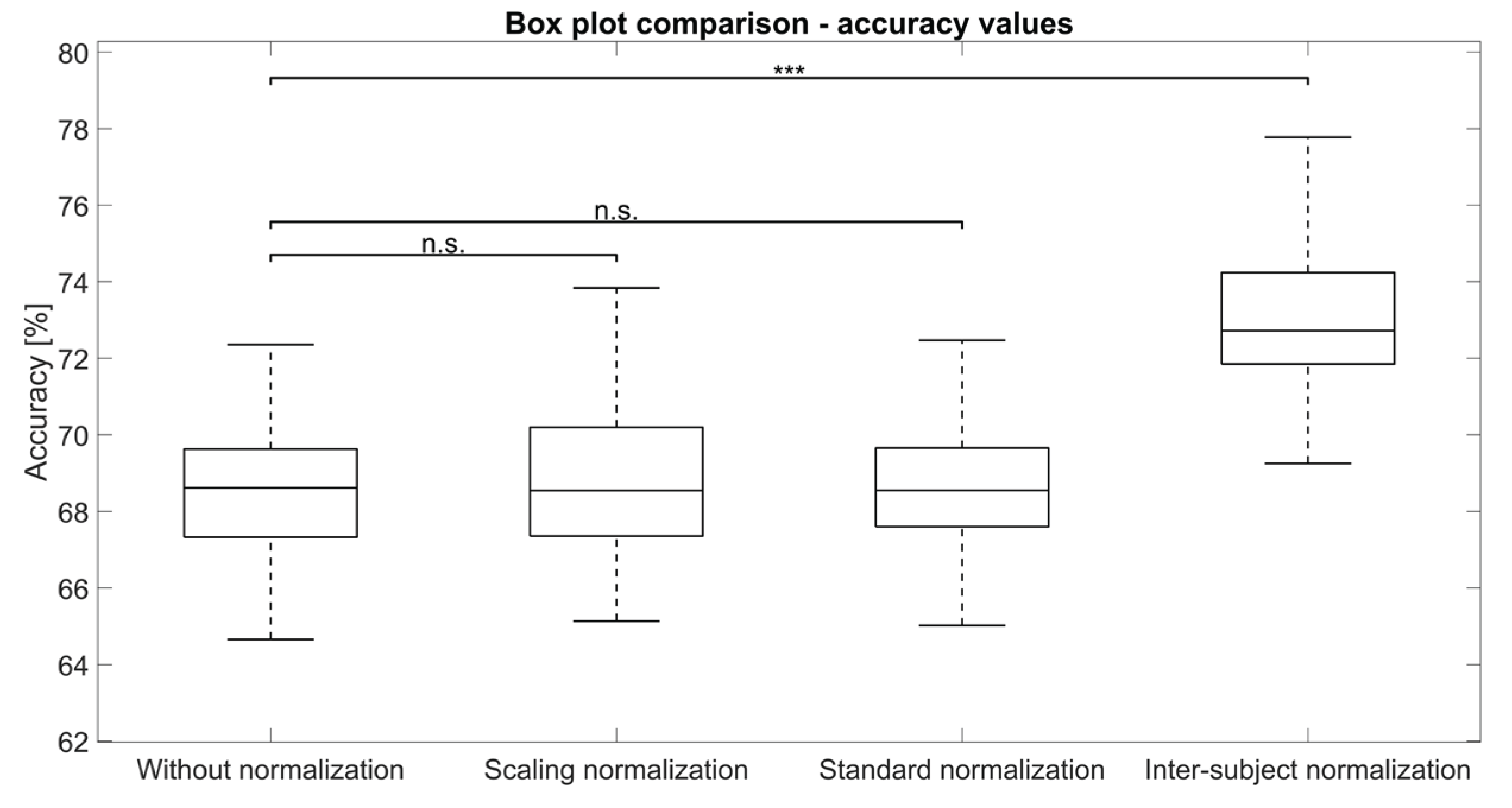

Table 1.
Heart rate derived from the original data and associated resampling frequencies in the subject-normalized domain.
Table 1.
Heart rate derived from the original data and associated resampling frequencies in the subject-normalized domain.
| Subject (n) |
Heart rate (beats per minute) |
Resampling frequency (Hz) |
|---|---|---|
| 1 | 67.3 | 260.0 |
| 2 | 66.2 | 264.4 |
| 3 | 80.7 | 216.9 |
| 4 | 71.9 | 243.4 |
| 5 | 61.3 | 285.5 |
| 6 | 76.6 | 228.5 |
| 7 | 61.4 | 285.0 |
| 8 | 60.7 | 288.3 |
| 9 | 83.7 | 209.1 |
| 10 | 62.4 | 280.4 |
Table 2.
Breath rate derived from the original data and associated resampling frequencies in the subject-normalized domain.
Table 2.
Breath rate derived from the original data and associated resampling frequencies in the subject-normalized domain.
| Subject (n) |
Breath rate (beats per minute) |
Resampling frequency (Hz) |
|---|---|---|
| 1 | 14.3 | 244.8 |
| 2 | 14.9 | 234.9 |
| 3 | 16.7 | 209.6 |
| 4 | 13.7 | 255.5 |
| 5 | 11.8 | 296.6 |
| 6 | 11.6 | 301.7 |
| 7 | 16.2 | 216.0 |
| 8 | 18.1 | 193.4 |
| 9 | 8.9 | 393.3 |
| 10 | 13.9 | 251.8 |
Table 3.
Performance obtained during classification using features derived from the original signals, features from the inter-subject normalized signals, standardized features, and scaled features. The characters ‘n.s.’ written as an apex denote no statistical significance, while three asterisks indicate statistical significance between the original data and the considered group. Significance was estimated comparing original data with other groups data.
| Metric | Original data | Standardization | Scaling | Inter-subject normalization |
|---|---|---|---|---|
| mean (SD) | mean (SD) | mean (SD) | mean (SD) | |
| Precision (%) | ||||
| Sensitivity (%) |
||||
| Specificity (%) | ||||
| Accuracy (%) |
Disclaimer/Publisher’s Note: The statements, opinions and data contained in all publications are solely those of the individual author(s) and contributor(s) and not of MDPI and/or the editor(s). MDPI and/or the editor(s) disclaim responsibility for any injury to people or property resulting from any ideas, methods, instructions or products referred to in the content. |
© 2025 by the authors. Licensee MDPI, Basel, Switzerland. This article is an open access article distributed under the terms and conditions of the Creative Commons Attribution (CC BY) license (http://creativecommons.org/licenses/by/4.0/).
Copyright: This open access article is published under a Creative Commons CC BY 4.0 license, which permit the free download, distribution, and reuse, provided that the author and preprint are cited in any reuse.


