Submitted:
01 September 2025
Posted:
03 September 2025
You are already at the latest version
Abstract
The relationship between humidity, pressure, temperature and wind speed measured at a network of stations on the Japanese islands and the seismic regime is studied for time 1973-2025. For each of the parameters, weighted average time series were constructed using the principal component method. Time series of weighted average parameters were subjected to wavelet decomposition. For wavelet decomposition levels the amplitudes of the envelopes and the points of their local extrema were found, which were compared with the times of earthquakes. The problem of estimating the advance measure of envelope extremum points relative to earthquake time moments was considered using a model of interacting point processes. For a sequence of 213 strong earthquakes with a magnitude of at least 6.5, the same number of the largest local maxima and the smallest local minima were selected for the extrema of envelopes amplitude of each parameter. It turned out that the largest advance measures occur for the 7th level of decomposition (periods from 16 to 32 days). Two advance mechanisms were identified: one mechanism is associated with the trigger effect of cyclones on seismicity, and the second with the occurrence of atmospheric earthquake precursors.
Keywords:
temperature
; humidity
; pressure
; wind speed
; earthquakes
; principal component analysis
; wavelets
; Hilbert transform
; coupled event intensity model
; Japan
1. Introduction
Changes in meteorological parameters associated with the preparation of earthquakes or occurring after seismic events have long been the subject of intensive research. These changes involve not only the atmosphere but also the electromagnetic fields in the ionosphere. In recent decades, these studies have led to the emergence of "new non-seismic precursors" that differ from traditional precursors associated with changes in the seismic regime, such as variations in the slope of the recurrence graph and oriented towards extracting information almost exclusively from seismic catalogues [1]. These precursors are considered to be the result of the interaction of many processes included in the global electric circuit and affecting air ionization and changes in the thermodynamic parameters of the atmosphere [2,3]. The general concept of the lithosphere-atmosphere-ionosphere interaction (LAIC) of the formation of short-term precursors as a result of the interaction of processes in the Earth's atmosphere, ionosphere and magnetosphere in the final stages of earthquake preparation is considered in [4,5]. From the point of view of the formation of precursors in the atmosphere, the key factor in these works is proposed to be considered as the ionization of air and the formation of water condensation nuclei by ions as a result of the action of radioactive radon on atmospheric gases. Radon emanation from the earth's interior occurs through the boundaries of the earth's crust blocks, including through active underwater tectonic faults. The application of this concept to the analysis of earthquake precursors is considered in articles [6,7]. In works [8,9,10], methods for analyzing radon emanation data (time series and spatial distribution) before strong earthquakes and for assessing potentially dangerous seismic areas are proposed based on the use of fractal statistics and power distribution laws.
Changes in the atmosphere are closely related to processes in the ionosphere. The works [11,12,13] study the electron density of the ionosphere, the formation of the distribution of electric potentials in the ionosphere and the features of electromagnetic ULF/ELF radiation before strong earthquakes, including the Tohoku mega-earthquake of March 11, 2011 in Japan. In the work [14] multiparameter observations before two strong earthquakes in Japan were analyzed from the point of view of the occurrence of low-frequency changes in the magnetic field, total electron content, as well as synchronous anomalous changes in meteorological parameters (temperature and humidity), which could be interpreted as precursors of seismic events. Similar studies are presented in the articles [15,16] before a series of earthquakes in New Zealand and Greece. In the work [17] using spectral and wavelet analysis the occurrence of an atmospheric gravity wave before an earthquake (M = 6.7) in India was studied. The occurrence of short-term precursors in China in the form of an anomalous vertical electric field of the atmosphere, due to the ionization of decay products of radioactive radon at different altitudes, was considered in the article [18]. In the work [19] it is shown that in the preparation zone of a large earthquake in Mexico (M=7.4), variations in temperature and relative humidity of the atmospheric air reach peak values within 10 days before the upcoming earthquake due to later disturbances of the total electron content in the ionosphere.
The occurrence of electrical impulses in the atmosphere in the vicinity of seismically active faults with subsequent air ionization and the formation of aerosols and ascending air currents was studied in [20]. Variations in the total electron content in the ionosphere before the earthquake in Haiti (M=7) were analyzed in [21] using parametric time series models and neural networks. The article [22] shows that some climatological anomalies may appear in the epicentral region weeks before large earthquakes. In particular, for several earthquakes in Central Italy, anomalies in temperature, water vapor and ozone content occurred within 2 months before the seismic events. The article [23] presents the results of detecting anomalies in air temperature, relative humidity and pressure that occurred one day before the seismic event in China. The article [24] shows that disturbances in atmospheric circulation in the form of interruption of climatic cyclone trajectories are a trigger for the occurrence of earthquake swarms in Iran. Similar studies on atmospheric processes such as abnormally low pressure, showers, storms and thunderstorms as triggers that provoke earthquakes in Japan are presented in [25].
The influence of the groundwater level and observed precipitation in the area of swarming earthquakes in southeastern Germany on the migration of hypocenters using the pore pressure diffusion model is presented in [26]. The problem of determining the most informative atmospheric and geochemical precursors in Japan for earthquakes with a magnitude of at least 6 is considered in [27]. The possibility of constructing a short-term forecast based on a model of interaction between the lithosphere, atmosphere and ionosphere was investigated in [28] using the example of a retrospective analysis of atmospheric parameters before a strong earthquake (M=7.8) in Mexico. The selection of short-term precursors based on the anomalous behavior of temperature, relative humidity and atmospheric chemical potential was studied in [29,30], including using the natural time apparatus to select critical behavior [29]. Similar studies are presented in [31] using the example of analyzing the processes of preparation for a strong seismic event in Altai. The use of satellite-based surface latent heat flux observations to extract the precursor behavior of large earthquakes (M=7.8, 7.3, 7.0) in Nepal and Japan using the natural time approach is presented in [32]. The analysis of surface latent heat flux together with atmospheric chemical potential for retrospective prediction of the Crete, Greece earthquake is presented in [33]. Multiparameter precursors of different physical nature describing the ionospheric and atmospheric states associated with the seismic event in Japan (M=7.1) are analyzed in [34] using several types of neural networks.
This work continues the study carried out in work [35] on the analysis of the relationships between anomalies of meteorological parameters (pressure, temperature and precipitation), recorded over a long period of time, from November 4, 1993 to September 30, 2024, with a time step of 3 hours, at the Pionerskaya meteorological station in Kamchatka with the seismic regime on the peninsula. In this study, the analysis was performed not for one station, but for a network of meteorological stations on the Japanese islands for a recording time of 52.5 years, from the beginning of 1973 to mid-2025.
2. Initial Data
The time series of temperature, humidity, barometric pressure and wind speed are freely available from https://www.ncei.noaa.gov/data/global-hourly/archive/csv/ . For meteorological stations belonging to Japan, the number of stations with available temperature data is 386, for humidity data the number of stations is 379, for barometric pressure 251 and for wind speed 387. The earliest start of the time series is dated back to 1946, but there are significant gaps in the data before 1973. Since 1973, the number of stations with available data increases sharply. Therefore, time series starting from 1973 with the longest gap duration not exceeding 0.5 year were further selected. The gaps were filled based on the behavior of the data to the left and right of the gap time interval in time segments whose length is equal to the gap length. The time series were then reduced to a uniform time step of 3 hours by averaging the data within successive 3-hour time intervals. As a result, time series of humidity for 111 stations, temperature for 112 stations, wind speed for 112 stations, and atmospheric pressure for 53 stations were obtained. The length of the obtained synchronous time series is 153452 readings with a step of 3 hours from the beginning of 1973 to July 7, 2025 (52.5 years).
For each meteorological parameter, the time series of the weighted average was calculated using the principal component method [36], in which the squares of the components of the eigenvector corresponding to the maximum eigenvalue of the correlation matrix of the multidimensional time series were taken as weights. By construction, the sum of the weights is equal to one. The station weight reflects the contribution of measurements made at the station to the overall average. In Figure 1, the positions of the meteorological stations for which the time series for humidity, temperature, wind speed and atmospheric pressure were used are shown in colored dots. The color of the dots reflects the rank of the station weight, which contributes to the calculation of the weighted average. A total of 6 ranks were used, for the calculation of which the range of change in weights for each parameter was divided into 6 intervals containing the same number of elements. On the maps shown in Figure 1, the remote station MINAMI TORISHIMA (Lat = 24.289697, Lon = 153.979119) stands out; its weight for all parameters belongs to the lowest rank.
Figure 2 shows the graphs of the average weighted time series of humidity, atmospheric pressure, temperature and wind speed. Once again, we note that these graphs represent one of the variants of the first principal component of the original multivariate time series.
3. Local Extremum Points of Envelopes After Wavelet Filtering
Each of the time series presented in Figure 2 was then subjected to decomposition into orthogonal components using a smooth 20th order symlet with 10 vanishing moments [37]. The choice of the optimal orthogonal wavelet was made based on the principle of minimum entropy of the distribution of the squared wavelet coefficients of all orthogonal Daubechies wavelets with a number of vanishing moments from 1 to 10.
The minimum period corresponding to the level of detail of the wavelet decomposition with number is , where is the time step of the time series. The maximum period of the level with number is . Since the time step is 3 hours, the range of periods for the 7th level varies from 384 to 768 hours, i.e. from 16 to 32 days.
For wavelet decompositions at level of detail number 7, the graphs of which are presented in Figure 3, their envelopes were calculated using the Hilbert transform [38].
To clarify these issues, we will apply the influence matrix method, which was previously used in [35,39,40,41] to analyze the relationships between the time moments of seismic events and the time points of local extremes of various statistics of meteorological time series, magnetic field fluctuations, earth surface tremors, and the influence of proton flux on the seismic process.
Figure 4.
The graphs are presented: (a) - moments of time of 213 earthquakes with a magnitude of at least 6.5; (b)-(e) - amplitudes of the envelopes of the wavelet components of the 7th level of detail of the weighted averages of humidity, atmospheric pressure, temperature and wind speed. The red dots on the graphs (b)-(e) mark the 213 largest local maxima of the envelopes of the 7th level of detail; the blue dots on the graphs (b)-(e) mark the 213 smallest local minima of the envelopes of the 7th level of detail.
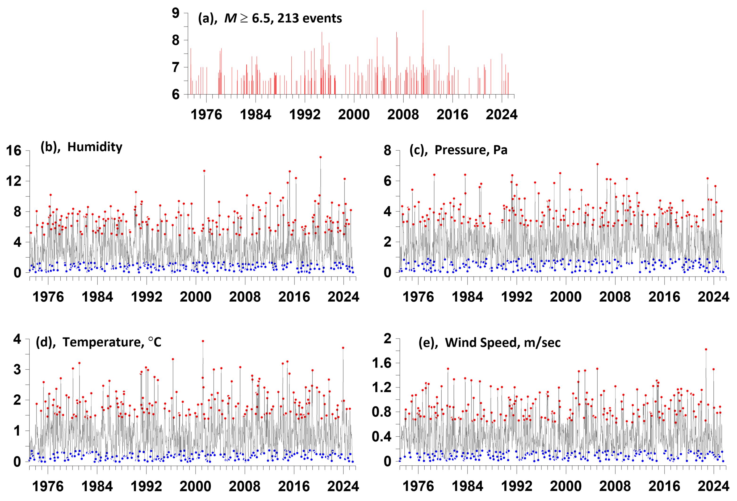
Figure 4(a) shows the time sequence of seismic events in the rectangular vicinity of the Japanese islands shown in Figure 1, with magnitudes of at least 6.5 for the time interval from the beginning of 1973 to July 7, 2025. Graphs 4(a, b, c, d) show the envelopes of the 7th level of the wavelet decomposition of the weighted average time series of humidity, pressure, temperature and wind speed and indicate the positions of the 213 most expressive local extrema of the envelopes: red dots - local maxima, blue dots - local minima.
4. Measures of Advance of Local Extrema of Envelope Time Moments with Respect to Times of Earthquakes
In what follows, we will be interested in the question of whether there is an advance of the times of the largest local maxima of the envelopes or the times of the smallest local minima of the envelopes of the 7th level of wavelet decompositions in Figure 4 with respect to time moments of earthquakes. In this case, we will separately consider the pairs of event sequences in Figure 4(a) and the largest local maxima of the envelopes of the 7th level of wavelet decompositions in Figure 4(b, c, d, e), red dots, and the smallest local minima of the envelopes in Figure 4(b, c, d, e), blue dots. In total, we will consider 4 pairs of time sequences, in which one of the sequences will always be the sequence of earthquakes with a minimum magnitude of 6.5, shown in Figure 4(a). Clarification of these issues requires also estimating the “reverse” advance and calculating their difference. If the average value of this difference is positive, then there is a trigger effect of the proton flux on seismicity. In addition, the value of the average difference of the lead measures will give a measure of the trigger effect.
To clarify these issues, we will apply the influence matrix method, which was previously used in [35,39,40,41] to analyze the relationships between the time moments of seismic events and the time points of local extremes of various statistics of meteorological time series, magnetic field fluctuations, earth surface tremors, and the influence of proton flux on the seismic process.
Let represent the moments of time of 2 event streams. In our case, these are:
1) a sequence of moments of time corresponding to the points of the most "expressive" local extrema of the envelopes of wavelet decompositions at the 7th level of detail;
2) a sequence of moments of time of earthquakes with a magnitude of at least 6.5.
Let us represent their intensities as follows:
where are the parameters, is the influence function of events of the flow with number :
According to formula (2), the weight of an event with number becomes non-zero for times and decays with characteristic time . The parameter determines the degree of influence of the event flow on the flow . The parameter determines the degree of influence of the flow on itself (self-excitation), and the parameter reflects a purely random (Poisson) component of intensity. Let us fix the parameter and consider the problem of determining the parameters The log-likelihood function for a non-stationary Poisson process is equal to over the time interval [42]:
It is necessary to find the maximum of functions (3) with respect to parameters . It can be shown that at the point of maximum of function (3) the condition is satisfied (for the derivation details see [35]):
Since the parameters must be non-negative, each term on the left-most part of this formula is zero at the point of maximum of function (3) – either due to the necessary conditions of the extremum (if the parameters are positive), or, if the maximum is reached at the boundary, then the parameters themselves are zero. Consequently, at the point of maximum of the likelihood function, the equality is satisfied:
Let's substitute the expression from (2) into (5) and divide by . Then we get another form of formula (5):
where . Substituting from (6) into (3), we obtain the following maximum problem:
where , subject to the following restrictions:
Having solved the problem (7-8) numerically for a given , we can enter the elements of the influence matrix according to the formulas:
The quantity is a part of the average intensity of the process with number , which is purely stochastic, the part is caused by the influence of self-excitation and is determined by the external influence . The normalization condition follows from formula (9):
As a result, we can determine the influence matrix:
The first column of matrix (11) is composed of Poisson fractions of mean intensities. The diagonal elements of the right submatrix of size 2×2 consist of self-excited elements of mean intensity, while the off-diagonal elements correspond to mutual excitation. The sums of the component rows of the influence matrix (11) are equal to 1. The influence matrices are estimated in a certain sliding time window of length with offset and with a given value of the attenuation parameter .
When analyzing variations of the components of influence matrices in sliding time windows corresponding to the mutual influence of the analyzed time sequences, the main attention is paid to their local maxima with their subsequent averaging. Below is described a method for processing these local maxima and averaging them for a set of time window lengths changing within specified limits.
1. The minimum and maximum lengths of time windows are selected and - the number of lengths of time windows in this interval. Thus, the lengths of time windows took the values , , , .
2. Each time window of length shifted from left to right along the time axis with some offset . Let us denote by , the sequence of time moments of the positions of the right windows of length . The number of time windows of length is determined by their time offset . We used a time window offset of 0.2 years.
3. For each position of the time window of length , the elements of the influence matrix (11) are estimated for a given relaxation time of the model (1), (2), corresponding to the mutual influence of the two analyzed processes. For definiteness, we will consider some one influence, for example, of the first process on the second. As a result of such estimates, we obtain their values in the form , where is the corresponding element of the influence matrix for the position with the number of the time window of length .
4. In the sequence , we select elements corresponding to local maxima of values , that is, from the condition .
5. We select a "small" time interval of length and for a sequence of such time fragments we calculate the average value of local maxima for which their time marks belong to these fragments. Averaging is performed over all lengths of time windows . In our calculations we took the length equal to 0.1 years.
5. Optimal Selection of Parameters and Two Advance Mechanisms
The complete set of free parameters of the influence matrix method is: , , , , , . The most critical for the calculation results is the choice of parameters , , . For each set of values , it is possible to calculate the average value of the lead measure between the moments of time of the most expressive local extrema of the envelopes relative to the moments of time of earthquakes and the average value of the inverse lead measure. We are interested in the difference of the average measures: . The choice of parameters was carried out from the condition:
The a priori limits of parameter variation in problem (12) were as follows (in years): , , , , , `. Problem (12) was solved numerically, using the random enumeration method, allowing parallel implementation of a large number of independent search flows (in total 3000 random trials for each variant) with the final selection of the best result.
As a result of calculating all the differences in the average lead measures for the optimal parameters found from the solution of problem (12), for the variants of sets of pairs of time moment sequences, those sequences of extremum points were selected for which the difference is maximum. The results of such a choice are presented in Table 1, which presents the optimal values of the parameters in years for all variants of the considered pairs of data and the corresponding maximum values of the difference .
The results of solving the problem (12) can be divided into 2 groups. The first group is a set of parameters of the model (1), (2), for which the value is maximum for each pair of local extremum points corresponding to each of the 4 meteorological quantities. This group corresponds to the points of local minimums of humidity, atmospheric pressure and temperature and the points of local maximums of wind speed. In Table 1, this group of parameters is highlighted in blue. The second group of parameters is made up of the remaining rows of Table 1, which are marked in black. The second group corresponds to the points of local maximums of humidity, pressure, temperature and the points of local minimums of wind speed.
The main difference between the first group and the second is the difference in the optimal values of the relaxation parameter found from the solution of problem (12) for humidity, pressure and temperature. In the first group, these values are 0.98, 0.98 and 0.78, while in the second group they are an order of magnitude greater: 9.74, 9.30 and 9.78.
Such a strong difference suggests that there are two physically different mechanisms of advance. We hypothesize that the first advance with small relaxation times (blue lines in Table 1) is related to the trigger mechanism of cyclone influence on the seismic process, since cyclones are characterized by low pressure, a drop in temperature, and increased wind. As for the second mechanism with large relaxation times (black lines in Table 1), we assume that it is related to the formation of atmospheric earthquake precursors [1,2,3,4,5,6,7,8,9,10,11,12,13,14,15,16,17,18,19,20,21,22,23,24,25,26,27,28,29,30,31,32,33,34], which are characterized by an increase in humidity and temperature as a result of the effect of radioactive radon on atmospheric gases and air ionization.
In the following, we will agree to call these two mechanisms the trigger and precursor advance. As can be seen from Table 1, the trigger atmospheric effect exceeds the precursor one, which is one of the reasons for the difficulties in detecting atmospheric precursors in practice.
The following Figure 5 shows the graphs of the change in the lead measures for all variants from Table 1. The left column of the graphs (blue) corresponds to the set of parameters from Table 1 that relate to the trigger mechanism of the lead, and the right column of the graphs (black) relates to the mechanism of the occurrence of atmospheric precursors.
6. Average Lead Measures
To highlight the general properties of the change in the lead measures separately for the trigger and precursor mechanisms, we average the curves in the left and right columns of Figure 5 in successive time fragments 0.1 years long and compare them with the graph of the logarithm of the released seismic energy calculated in a sliding time window of 1 year length also with a shift of 0.1 years for all earthquakes. The results of such calculations are presented in Figure 6.
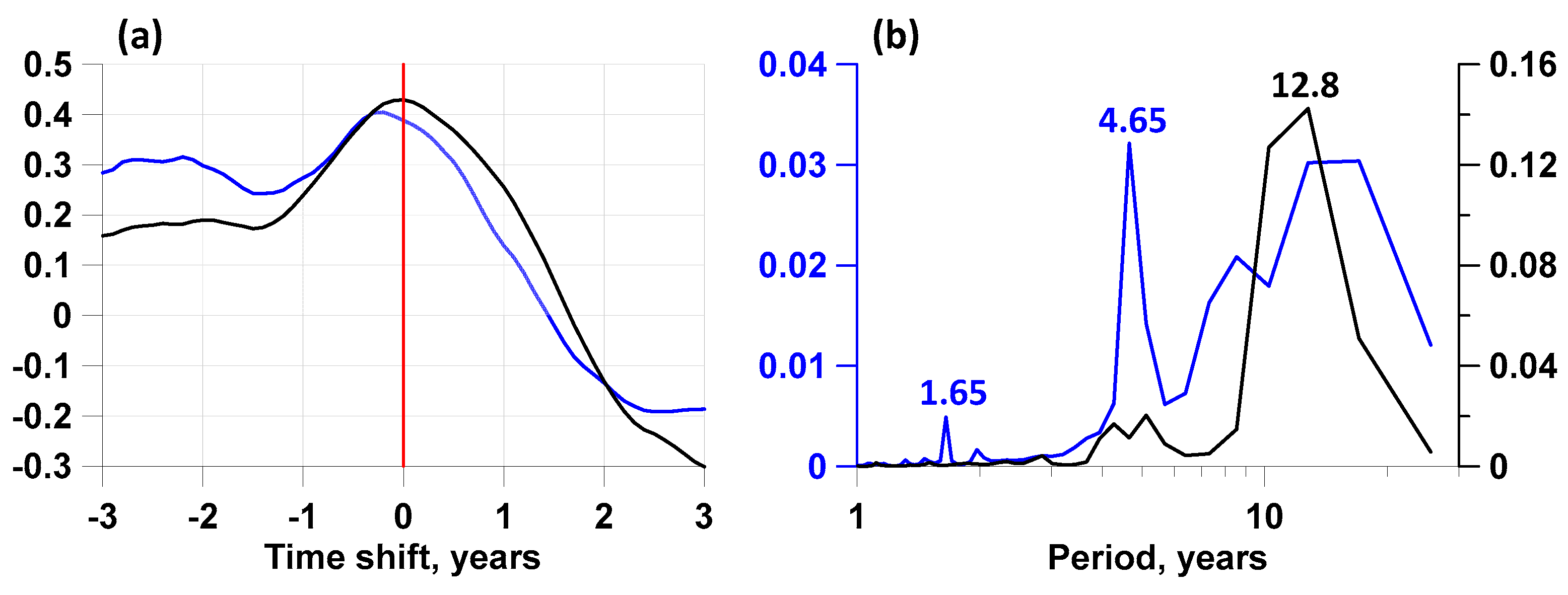
It is of interest to estimate the extent to which the curves of the change in the average lead measures in Figure 6(b, c) themselves additionally lead the seismic energy emissions shown in Figure 6(a). To do this, we calculate the correlation coefficients between the values of the logarithm of the discharged seismic energy (Figure 6(a)) and the average lead measures (Figure 6(b, c)), where is the discrete time index. We calculate the correlation coefficients between and , where the time shift changes within certain limits , that is, the correlation function. Due to the fact that the correlated values in Figure 6 differ greatly from the Gaussian ones, we will use the Spearman rank correlation coefficient [43]. Figure 6(a) shows the graphs of the Spearman correlation functions , the angle brackets mean the calculation of the correlation coefficient. The limits of the change in the time shift were taken from -3 to +3 years. From the graphs in Figure 7(a) it can be seen that the correlation functions are strongly asymmetric and shifted towards negative values, which means that the variations in the average measures of advancement of changes in the release of seismic energy are ahead.
In addition, Figure 7(b) presents the graphs of the estimates of the power spectra of the curves of the change in the average lead measures and indicates the periods corresponding to the spectral peaks. The spectral peak with a period of 12.8 years, which is close to the period of solar activity, is noteworthy. This spectral peak is most strongly expressed for the average lead measure in Figure 6(c), corresponding to the second lead mechanism with large values of the relaxation parameter , presumably associated with the formation of atmospheric precursors.
7. Discussion
This section is not mandatory but may be added if there are patents resulting from the work reported in this manuscript.
A method is proposed for analyzing a large number of long-term meteorological time series measured at a network of stations to compare their anomalies with the seismic regime. Data processing is based on the sequential application of the principal component method, wavelet decomposition, calculation of envelopes using the Hilbert transform, and application of a parametric model of coupled point processes to the points of local extrema of the envelope amplitudes and the sequence of seismic events.
The method is illustrated by the example of the analysis of data from a network of meteorological stations in Japan for the time period from early 1973 to mid-2025. As a result of the analysis, two mechanisms were discovered for the advance of local extremum points of the amplitudes of the envelopes of the wavelet decomposition of time series of humidity, pressure, temperature and wind speed at the low-frequency 7th level of detail (periods from 16 to 32 days) relative to the time moments of earthquakes with a magnitude of at least 6.5. The mechanisms differ in the values of the optimal relaxation time of the model of interacting point processes by an order of magnitude.
The first mechanism, which was classified as triggering, is characterized by the advance of local minimum humidity, pressure and temperature points and local maximum wind speed points relative to the time of seismic events. Its cause is the triggering effect of cyclones on the occurrence of earthquakes.
The second mechanism, which was classified as a precursor, is characterized by the advance of local maximums of humidity, pressure and temperature and local minimums of wind speed relative to the time of seismic events. Its cause is the occurrence of atmospheric precursors as a result of the impact of radioactive radon, released from faults in the earth's crust before earthquakes, on atmospheric gases and the subsequent ionization of air.
The averaged lead curves for both mechanisms also lead the seismic energy release calculated for all earthquakes, as follows from the asymmetry of the Spearman correlation function.
For the averaged curve of the precursor-type lead measure, a strong periodicity with a period close to the period of solar activity was discovered.
Author Contributions
A.L.—ideating the research, writing the text, data processing; E.R.—data preparation. All authors have read and agreed to the published version of the manuscript.
Funding
This research received no external funding.
Institutional Review Board Statement
Not applicable.
Informed Consent Statement
Not applicable.
Data Availability Statement
The original meteorological data are contained in the database by the address https://www.ncei.noaa.gov/data/global-hourly/archive/csv/ (accessed on 15 July 2025). The information about seismic process was taken from the site https://earthquake.usgs.gov/earthquakes/search (accessed on 15 July 2025).
Acknowledgments
This work was carried out within the framework of the state assignments of the Institute of Physics of the Earth of the Russian Academy of Sciences.
Conflicts of Interest
The authors declare that the research was conducted in the absence of any commercial or financial relationships that could be construed as a potential conflict of interest.
References
- Tritakis: V. Seismicity Precursors and their Practical Account. Geosciences 2025, 15, 147. [CrossRef]
- Pulinets, S.; Herrera, V.M.V. Earthquake Precursors: The Physics, Identification, and Application. Geosciences 2024, 14, 209. [CrossRef]
- De Santis, A.; Abbattista, C.; Alfonsi, L.; Amoruso, L.; Campuzano, S.A.; Carbone, M.; Cesaroni, C.; Cianchini, G.; De Franceschi, G.; De Santis, A.; et al. Geosystemics View of Earthquakes. Entropy 2019, 21, 412. [CrossRef]
- Pulinets, S.A.; Ouzounov, D.P.; Karelin, A.V.; Davidenko, D.V. Physical bases of the generation of short-term earthquake precursors: A complex model of ionization-induced geophysical processes in the lithosphere-atmosphere-ionosphere-magnetosphere system. Geomagn. Aeron. 2015, 55, 521-538. [CrossRef]
- Pulinets, S.; Ouzounov, D. Lithosphere-Atmosphere-Ionosphere Coupling (LAIC) model - An unified concept for earthquake precursors validation. J. Asian Earth Sci. 2011, 41, 371-382. [CrossRef]
- Dunajecka, M.A.; Pulinets, S.A. Atmospheric and thermal anomalies observed around the time of strong earthquakes in Mexico. Atmosfera 2005, 18, 235-247.
- Ouzounov, D.; Pulinets, S.; Kafatos, M.C.; Taylor, P. Thermal Radiation Anomalies Associated with Major Earthquakes. In Pre-Earthquakes Processes: A Multidisciplinary Approach to Earthquake Prediction Studies, AGU Geophysical Monograph Series; John Wiley & Sons Inc.: New York, NY, USA, 2018; Volume 234, pp. 259-274. [CrossRef]
- Nikolopoulos, D.; Cantzos, D.; Alam, A.; Dimopoulos, S.; Petraki, E. Electromagnetic and Radon Earthquake Precursors. Geosciences 2024, 14, 271. [CrossRef]
- Alam, A.; Nikolopoulos, D.; Wang, N. Fractal Patterns in Groundwater Radon Disturbances Prior to the Great 7.9 Mw Wenchuan Earthquake, China. Geosciences 2023, 13, 268. [CrossRef]
- Omori, Y.; Yasuoka, Y.; Nagahama, H.; Kawada, Y.; Ishikawa, T.; Tokonami, S.; Shinogi, M. Anomalous radon emanation linked to preseismic electromagnetic phenomena. Nat. Hazards Earth Syst. Sci. 2007, 7, 629-635. [CrossRef]
- Lukianova, R.; Daurbayeva, G.; Siylkanova, A. Ionospheric and Meteorological Anomalies Associated with the Earthquake in Central Asia on 22 January 2024. Remote Sens. 2024, 16, 3112. [CrossRef]
- Lukianova, R.; Christiansen, F. Modeling of the global distribution of ionospheric electric fields based on realistic maps of field-aligned currents. J. Geophys. Res. 2006, 111, A03213. [CrossRef]
- Hayakawa, M.; Izutsu, J.; Schekotov, A.; Yang, S.-S.; Solovieva, M.; Budilova, E. Lithosphere-atmosphere-ionosphere coupling effects based on multiparameter precursor observations for February-March 2021 earthquakes (M~7) in the offshore of Tohoku area of Japan. Geosciences 2021, 11, 481. [CrossRef]
- Hayakawa, M.; Schekotov, A.; Izutsu, J.; Yang, S.-S.; Solovieva, M.; Hobara, Y. Multi-Parameter Observations of Seismogenic Phenomena Related to the Tokyo Earthquake (M = 5.9) on 7 October 2021. Geosciences 2022, 12, 265. [CrossRef]
- Adil, M.A., Abbas, A., Ehsan, M., Shah, M., Naqvi, N.A., Alie, A., Investigation of ionospheric and atmospheric anomalies associated with three Mw > 6.5 EQs in New Zealand. J. Geodyn. 2021, 145, 101841 . [CrossRef]
- Sasmal, S.; Chowdhury, S.; Kundu, S.; Politis, D.Z.; Potirakis, S.M.; Balasis, G.; Hayakawa, M.; Chakrabarti, S.K. Pre-Seismic Irregularities during the 2020 Samos (Greece) Earthquake (M = 6.9) as Investigated from Multi-Parameter Approach by Ground and Space-Based Techniques. Atmosphere 2021, 12, 1059. [CrossRef]
- Biswas, S., Kundu, S., Ghosh, S., Chowdhury, S., Yang, S.-S., Hayakawa, M., Chakraborty, S., Chakrabarti, S.K. and Sasmal, S. Contaminated Effect of Geomagnetic Storms on Pre-Seismic Atmospheric and Ionospheric Anomalies during Imphal Earthquake. Open Journal of Earthquake Research, 2020, 9, 383-402. [CrossRef]
- Han, R.; Cai, M.; Chen, T.; Yang, T.; Xu, L.; Xia Q.; Jia, X.; Han, J. Preliminary Study on the Generating Mechanism of the Atmospheric Vertical Electric Field before Earthquakes. Appl. Sci. 2022, 12, 6896. [CrossRef]
- Salh H., Muhammad A., Ghafar M.M., Kulahci F. Potential utilization of air temperature, total electron content, and air relative humidity as possible earthquake precursors: A case study of Mexico M7.4 earthquake. Journal of Atmospheric and Solar-Terrestrial Physics 2022, 237, 105927, . [CrossRef]
- Liperovsky, V.A.; Meister, C.V.; Liperovskaya, E.V.; Davidov, V.F.; Bogdanov, V.V. On the possible influence of radon and aerosol injection on the atmosphere and ionosphere before earthquakes. Nat. Hazards Earth Syst. Sci. 2005, 5, 783-789. [CrossRef]
- Saqib, M., Sent?rk, E., Sahu, S.A., Adil, M.A., Comparisons of autoregressive integrated moving average (ARIMA) and long short term memory (LSTM) network models for ionospheric anomalies detection: a study on Haiti (Mw = 7.0) earthquake. Acta Geodaetica et Geophysica 2022, 57 (1), 195-213. [CrossRef]
- Piscini, A., De Santis, A., Marchetti, D., Cianchini, G., A multi-parametric climatological approach to study the 2016 amatrice-norcia (Central Italy) earthquake preparatory phase. Pure Appl. Geophys. 2017, 174 (10), 3673-3688. [CrossRef]
- Jing, F., Shen, X. H., Kang, C. L., and Xiong, P.: Variations of multi-parameter observations in atmosphere related to earthquake, Nat. Hazards Earth Syst. Sci., 2013, 13, 27-33, . [CrossRef]
- Daneshvar, M.R.M.; Tavousi, T.; Khosravi, M., M. Atmospheric blocking anomalies as the synoptic precursors prior to the induced earthquakes: a new climatic conceptual model. Int. J. Environ. Sci. Technol. 2015, 12, 1705-1718. [CrossRef]
- Freund, F.T.; Mansouri, Daneshvar, M.R.; Ebrahimi, M. Atmospheric Storm Anomalies Prior to Major Earthquakes in the Japan Region. Sustainability 2022, 14, 10241. [CrossRef]
- Kraft T., Wassermann J., Schmedes E., Igel H. Meteorological triggering of earthquake swarms at Mt. Hochstaufen, SE-Germany. Tectonophysics 2006, 424, 245-258. [CrossRef]
- Genzano, N.; Filizzaola, C.; Hattori, K.; Pergola, N.; Tramutoli, V. Statistical correlation analysis between thermal infrared anomalies observed from MTSATs and large earthquakes occurred in Japan (2005-2015). J. Geophys. Res. Solid Earth 2021, 126, e2020-JB020108. [CrossRef]
- Pulinets, S. A., Ouzounov, D., Ciraolo, L., Singh, R., Cervone, G., Leyva, A., Dunajecka, M., Karelin, A. V., Boyarchuk, K. A., and Kotsarenko, A.: Thermal, atmospheric and ionospheric anomalies around the time of the Colima M7.8 earthquake of 21 January 2003, Ann. Geophys., 2006, 24, 835-849, . [CrossRef]
- Hayakawa, M., Potirakis, S.M., Hirooka, S. and Hobara, Y. Meteorological Anomalies Based on Ground-Based AMeDAS Data for the 1995 Kobe Earthquake: Critical Natural Time Analysis. Open Journal of Earthquake Research, 2025, 14, 67-84. [CrossRef]
- Pulinets, S.; Budnikov, P. Atmosphere Critical Processes Sensing with ACP. Atmosphere 2022, 13, 1920. [CrossRef]
- Shitov, A.V.; Pulinets, S.A.; Budnikov, P.A. Effect of Earthquake Preparation on Changes in Meteorological Characteristics (Based on the Example of the 2003 Chuya Earthquake). Geomagn. Aeron. 2023, 63, 395-408. [CrossRef]
- Ghosh, S.; Chowdhury, S.; Kundu, S.; Sasmal, S.; Politis, D.Z.; Potirakis, S.M.; Hayakawa, M.; Chakraborty, S.; Chakrabarti, S.K. Unusual Surface Latent Heat Flux Variations and Their Critical Dynamics Revealed before Strong Earthquakes. Entropy 2022, 24, 23. [CrossRef]
- Ghosh, S.; Sasmal, S.; Maity, S.K.; Potirakis, S.M.; Hayakawa, M. Thermal Anomalies Observed during the Crete Earthquake on 27 September 2021. Geosciences 2024, 14, 73. [CrossRef]
- Draz, M.U.; Shah, M.; Jamjareegulgarn, P.; Shahzad, R.; Hasan, A.M.; Ghamry, N.A. Deep Machine Learning Based Possible Atmospheric and Ionospheric Precursors of the 2021 Mw 7.1 Japan Earthquake. Remote Sens. 2023, 15, 1904. [CrossRef]
- Lyubushin, A.; Kopylova, G.; Rodionov, E.; Serafimova, Y. An Analysis of Meteorological Anomalies in Kamchatka in Connection with the Seismic Process. Atmosphere 2025, 16, 78. [CrossRef]
- Jolliffe, I.T. Principal Component Analysis; Springer: Berlin/Heidelberg, Germany, 1986.
- Mallat, S.A. Wavelet Tour of Signal Processing, 2nd ed.; Academic Press: Cambridge, MA, USA, 1999.
- Bendat, J.S.; Piersol, A.G. Random Data. Analysis and Measurement Procedures, 4th ed.; Wiley & Sons: Hoboken, NJ, USA, 2010.
- Lyubushin, A.; Rodionov, E. Prognostic Properties of Instantaneous Amplitudes Maxima of Earth Surface Tremor. Entropy 2024, 26, 710. [CrossRef]
- Lyubushin, A.; Rodionov, E. Wavelet-based correlations of the global magnetic field in connection to strongest earthquakes. Adv. Space Res. 2024, 74, 3496-3510. [CrossRef]
- Lyubushin, A.; Rodionov, E. Quantitative Assessment of the Trigger Effect of Proton Flux on Seismicity. Entropy 2025, 27, 505. [CrossRef]
- Cox, D.R.; Lewis, P.A.W. The Statistical Analysis of Series of Events; Methuen: London, UK, 1966.
- Kendall, M.G.; Stuart, A. The Advanced Theory of Statistics, Volume 2: Inference and Relationship. Griffin. 1973.
Figure 1.
Locations of meteorological stations for humidity, temperature, wind speed and atmospheric pressure, for which time series with a time step of 3 hours were generated, starting from 1973 to mid-2025. The color scheme of the dots reflects the 6 ranks of the measurement of the weights of the time series from the stations, which were used to calculate the weighted average for each of the 4 meteorological parameters.
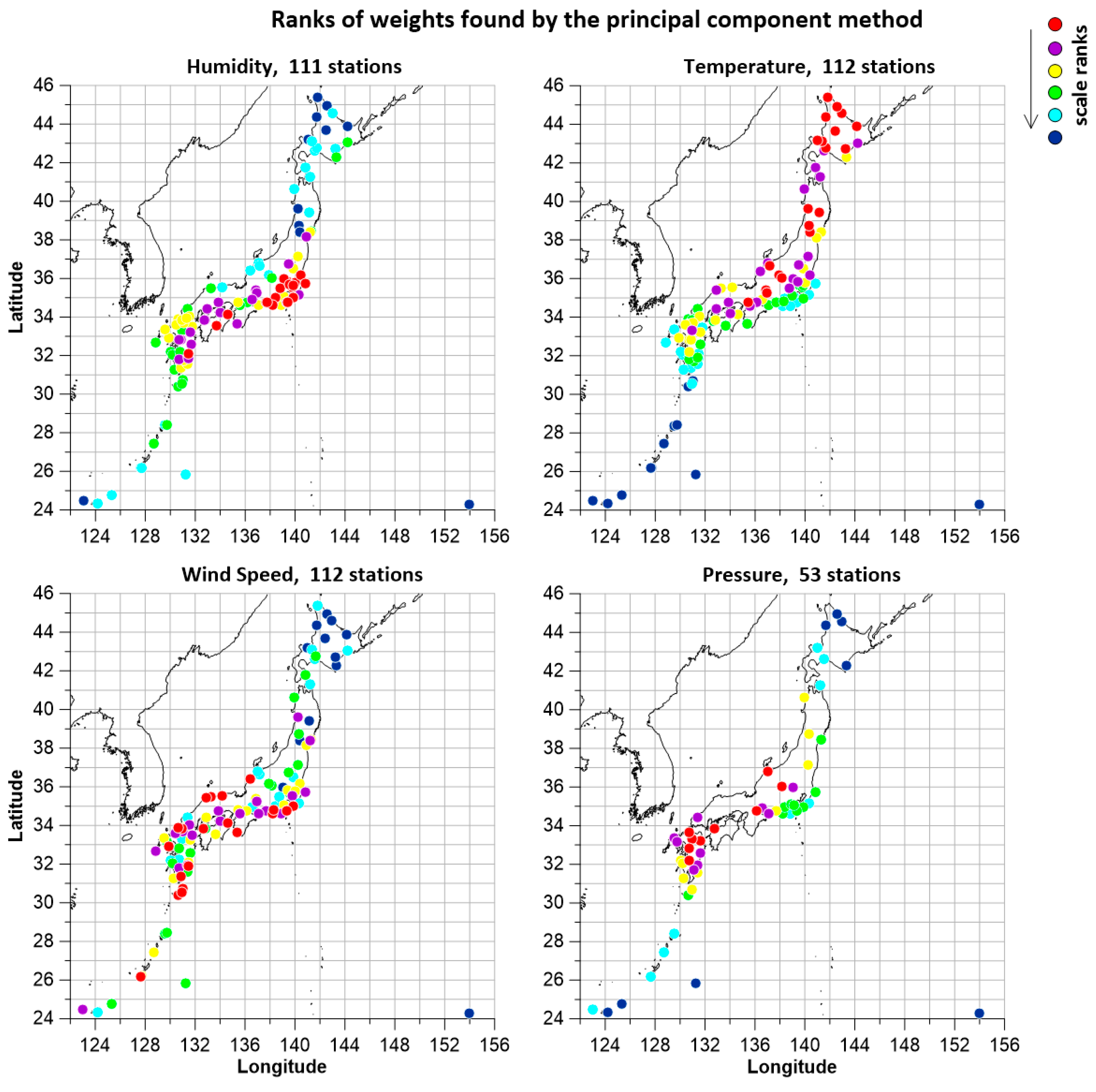
Figure 2.
Graphs of weighted average humidity, temperature, atmospheric pressure and wind speed for the network of meteorological stations on the Japanese islands.
Figure 2.
Graphs of weighted average humidity, temperature, atmospheric pressure and wind speed for the network of meteorological stations on the Japanese islands.
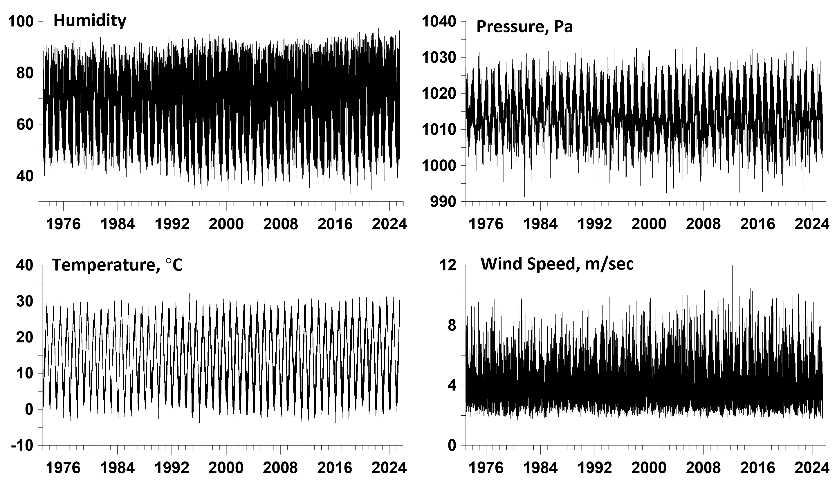
Figure 3.
Graphs of the wavelet decomposition components of weighted average meteorological parameters corresponding to detail level number 7.
Figure 3.
Graphs of the wavelet decomposition components of weighted average meteorological parameters corresponding to detail level number 7.
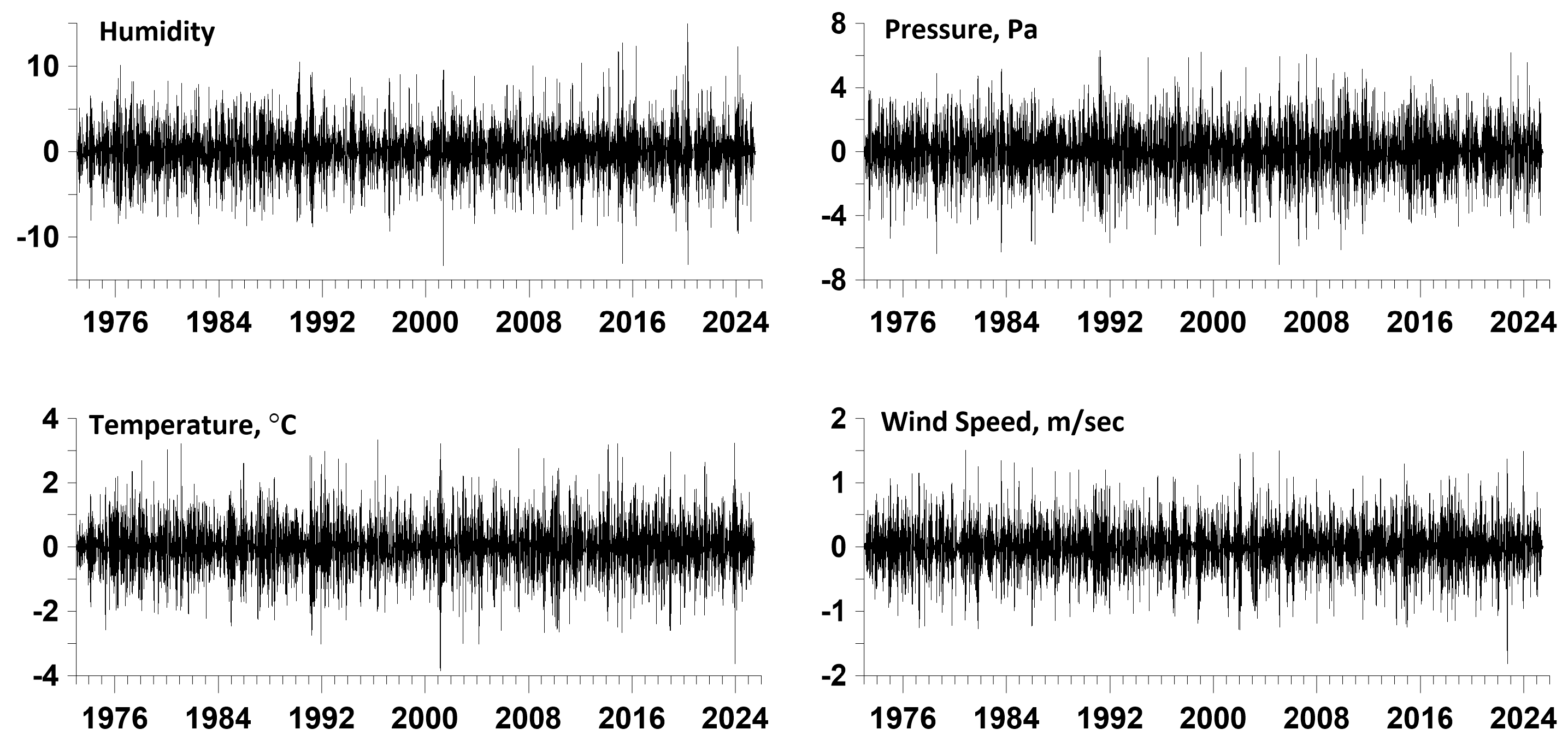
Figure 5.
The left column of graphs (blue lines), in figures (a1, b1, c1, d1) presents graphs of the lead measures (for the variants with the highest average values in Table 1) by the time points of the smallest local minima (a1, b1, c1) for the amplitudes of the humidity, pressure and temperature envelopes and the largest local maxima (d1) for wind speed relative to the time moments of earthquakes with magnitudes not lower than 6.5. The right column of graphs (black lines), in figures (a2, b2, c2, d2) presents graphs of the lead measures by the time points of the largest local maxima (a2, b2, c2) for the amplitudes of the humidity, pressure and temperature envelopes and the smallest local minima (d2) for wind speed relative to the time moments of earthquakes with magnitudes not lower than 6.5. All graphs show the values of optimal relaxation times , horizontal red lines and red numbers show the average values of the lead measures.
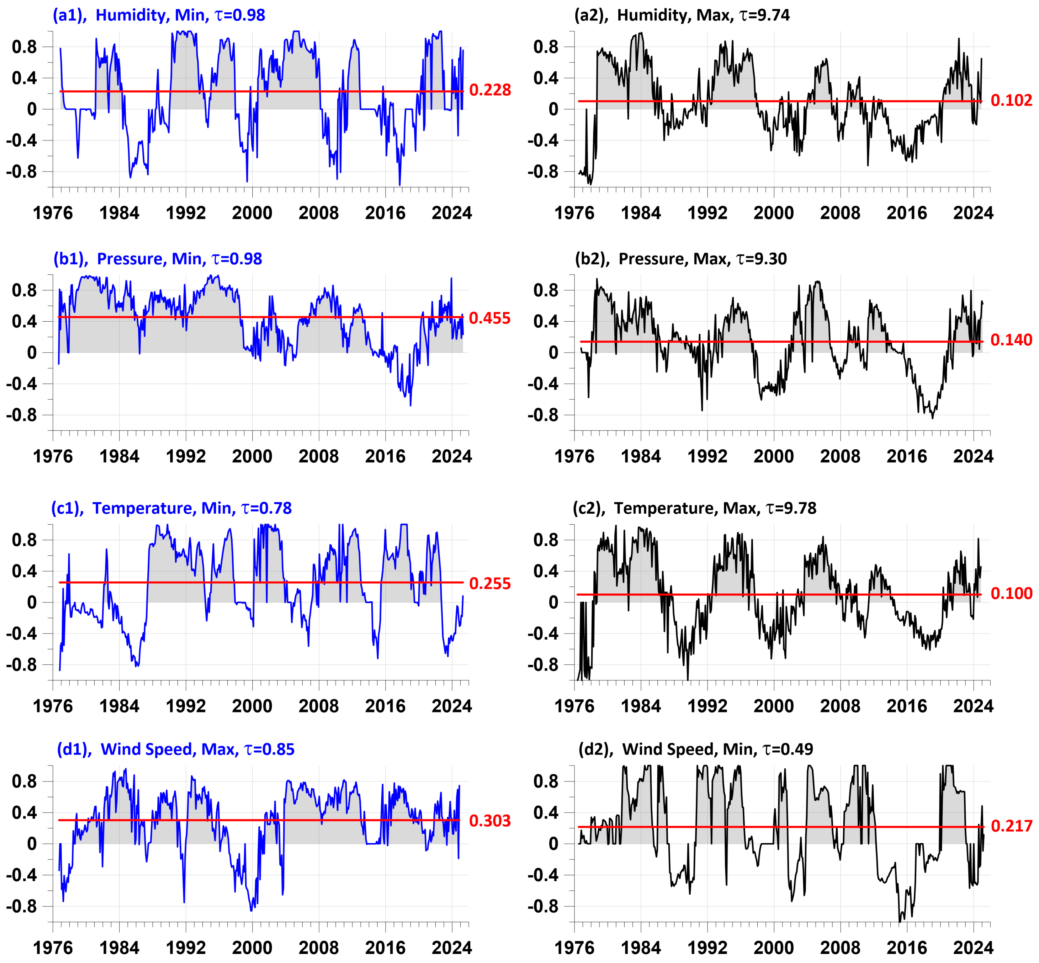
Figure 6.
Graph (a) presents the values of the logarithms of the released seismic energy (in joules) in a 365-day window with a shift of 36 days. Graph (b), blue line, presents the average measure of lead by the time points of the most pronounced local extremes of the amplitudes of the envelopes of four meteorological parameters relative to the time points of earthquakes with magnitudes not lower than 6.5 for the variants with the highest average values in Table 1. Graph (c), black line, presents the average measure of lead by the time points of the most pronounced local extremes of the amplitudes of the envelopes of four meteorological parameters relative to the time points of earthquakes with magnitudes not lower than 6.5 for the variants with the lowest average values in Table 1. The horizontal red lines and red numbers show the average values of the average measures of lead.
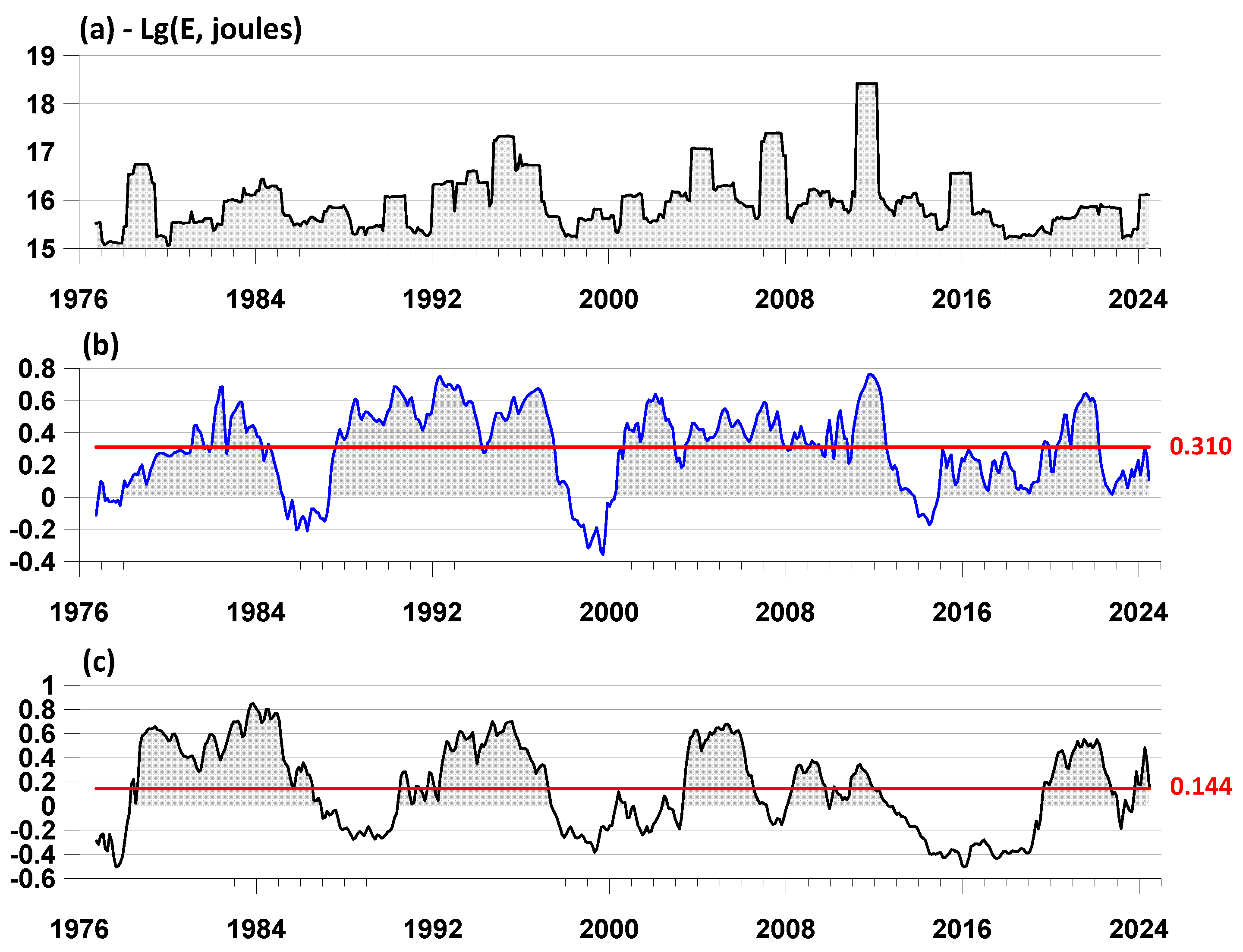
Figure 7.
In Figure 7(a), the blue line is the plot of the Spearman correlation function between the seismic energy release in a 365-day window with a 36-day shift (Figure 6(a)) and the average lead curve of the most pronounced local extremes for the variants with the highest average values in Table 1 of the amplitudes of the envelopes of the four meteorological parameters relative to the times of earthquakes with magnitudes not lower than 6.5 (Figure 6(b)). The black line in Figure 7(a) is the plot of the Spearman correlation function between the seismic energy release and the average lead time of the most pronounced local extremes for the variants with the lowest average values in Table 1 of the amplitudes of the envelopes of the four meteorological parameters relative to the times of earthquakes with magnitudes not lower than 6.5 (Figure 6(c)). Figure 7(b) shows graphs of estimates of the power spectra of the curves of changes in the average lead measures in Figure 6(a) and 6(b), respectively (blue and black lines); the numbers indicate the periods of the spectral peaks.

| Property | ||||
| Humidity, Max | 9.74 | 2.84 | 7.59 | 0.102 |
| Humidity, Min | 0.98 | 2.60 | 4.00 | 0.228 |
| Pressure, Max | 9.30 | 2.92 | 7.97 | 0.140 |
| Pressure, Min | 0.98 | 2.81 | 8.04 | 0.455 |
| Temperature, Max | 9.78 | 2.52 | 8.65 | 0.100 |
| Temperature, Min | 0.78 | 2.99 | 4.69 | 0.255 |
| Wind Speed, Max | 0.85 | 2.93 | 5.92 | 0.303 |
| Wind Speed, Min | 0.49 | 2.97 | 4.11 | 0.217 |
Disclaimer/Publisher’s Note: The statements, opinions and data contained in all publications are solely those of the individual author(s) and contributor(s) and not of MDPI and/or the editor(s). MDPI and/or the editor(s) disclaim responsibility for any injury to people or property resulting from any ideas, methods, instructions or products referred to in the content. |
© 2025 by the authors. Licensee MDPI, Basel, Switzerland. This article is an open access article distributed under the terms and conditions of the Creative Commons Attribution (CC BY) license (http://creativecommons.org/licenses/by/4.0/).
Copyright: This open access article is published under a Creative Commons CC BY 4.0 license, which permit the free download, distribution, and reuse, provided that the author and preprint are cited in any reuse.


