
Submitted:
01 September 2025
Posted:
02 September 2025
You are already at the latest version
Abstract
Ultraslow diffusion (slow subdiffusion) is usually defined as a random walk of a diffusing molecule such that its mean square displacement is controlled by a slowly varying function, in practice, by a combination of logarithmic functions. The Green’s function describing molecule diffusion is often determined in the long-time limit. We show that the g-subdiffusion equation with the fractional Caputo derivative with respect to another function g describes ultraslow diffusion in the entire time domain when the function g is appropriately chosen. To determine the Green’s function we use a method based on the Laplace transform with respect to the function g. We also use the g-subdiffusion equation to model a continuous transition between two different ultraslow diffusion processes.
Keywords:
ultraslow diffusion
; g-subdiffusion equation
; fractional Caputo derivative with respect to another function
; anomalous diffusion
; fractional calculus
1. Introduction
Most often, the type of diffusion is defined by the temporal evolution of the mean square displacement (MSD) of a diffusing molecule . When MSD is a power function of time, , then is for superdiffusion, for normal diffusion, and for subdiffusion [1,2,3,4,5]. The equations describing these processes can be derived within the continuous time random walk (CTRW) model [3,5,6]. Superdiffusion (facilitated diffusion) occurs when anomalously long molecule jumps can be performed with high probability, which occurs in turbulent media. This process is described by the superdiffusion equation with a fractional derivative with respect to spatial variable. Subdiffusion (hindered diffusion) occurs when the waiting time for a molecule to jump is anomalously long, which occurs, for example, in gels, bacterial biofilms, porous materials, dense polymer solutions, and crowded intracellular spaces like the cytoplasm and cell membranes, see [3,4,5,7,8,9,10,11,12,13,14,15]. Subdiffusion is described by an equation with a fractional derivative with respect to time [3,4,5,16,17].
The above examples are not a complete list of types of anomalous diffusion. One of the processes other than those mentioned above is ultraslow diffusion (slow subdiffusion), for which when , where is a slowly varying function which, in practice, is a combination of logarithmic functions [18,19,20]. This process is significantly slower than ordinary subdiffusion. Although ultraslow diffusion and ordinary subdiffusion are qualitatively different, it is rather difficult to distinguish them from experimental data (especially when is close to zero) unless these processes are considered over sufficiently long times. Ultraslow diffusion occurs when the movement of diffusing objects is extremely hindered, as in very crowded systems. The process has been observed in systems with extreme levels of heterogeneity and disorder. The examples are water transport in sucrose glasses at low temperatures [21], diffusion in highly congested media where particle motion is nearly arrested, and the dynamics of language, where the usage frequency of common words evolves logarithmically [22].
There exists experimental evidence in numerous systems for logarithmically slow time evolution, yet its full theoretical understanding remains elusive. In [23] there have been introduced and studied a generic transition process in complex systems, based on non-renewal, aging waiting times. This model provides a universal description for transition dynamics between aging and nonaging states. In [24] the authors develop the stochastic foundations for ultraslow diffusion based on random walks with a random waiting time between jumps whose probability tail falls off at a logarithmic rate. The Sinai model describes motion in a random potential [25,26]. Theoretical and simulation studies have generalized this result, showing that ultraslow diffusion appears in stationary Gaussian potentials with spatially vanishing correlations, provided the temperature is sufficiently low or the disorder is strong [20]. In [27] the authors use the inverse Mittag-Leffler function as the function in the structural derivative modeling ultraslow diffusion of a random system of two interacting particles. It has been noticed that the dynamics of two interacting particles are respectively the ballistic motion at the short time scale and the Sinai ultraslow diffusion at the long time scale [25]. Ultraslow-like behavior has been observed in aging colloidal glasses, where the nature of diffusion can be tuned by changing the density and heterogeneity of the system. Logarithmic aging phenomena, in which the relaxation of the system progresses logarithmically with time, are widespread in disordered materials and provide strong evidence of underlying ultraslow dynamics [28]. Another example is momentum space diffusion in billiard systems with specific geometry (e.g., a right triangle), where chaotic dynamics leads to a logarithmic increase in the MSD [29]. A medium in which ultraslow diffusion occurs may change over time due to changes in the medium structure or in external factors, such as temperature. Ultraslow diffusion in a medium with parameters changing over time was considered in [26].
In systems dominated by extreme heterogeneity, hierarchical energy landscapes, or long-range memory effects, classical diffusion and even ordinary subdiffusion models may prove insufficient. The study of ultraslow diffusion opens new perspectives for understanding dynamics in systems far from equilibrium, ranging from aging processes in amorphous materials to the evolution of complex social and informational networks.
To describe ultraslow diffusion we will use the g-subdiffusion equation with an appropriately chosen function g. This equation contains the time-fractional Caputo derivative with respect to the function g. The g-subdiffusion equation was first used in the paper [30] to model the smooth transition from ordinary subdiffusion to ultraslow diffusion. It has also been used to model superdiffusion [31], subdiffusion with anomalous decay of diffusing molecules [32], smooth transitions from subdiffusion to superdiffusion [33], and transition between two different subdiffusion processes [34]. A stochastic interpretation of the g-subdiffusion process is shown in [35]. The g-subdiffusion equation can be treated as a fairly general anomalous diffusion equation with certain restrictions imposed on the function g, see also [36].
The paper is organized as follows. Section 2 presents the basics of the standard model of anomalous diffusion, namely the continuous-time random walk model. It is shown how the Laplace transform of the distribution of the waiting time for a particle to jump determines the subdiffusion equation, its Green’s function, and the time evolution of MSD. The derivation of the ordinary subdiffusion equation and its Green’s function is shown in Section 3. In Section 4, the general form of the Green’s function and the time evolution of the MSD for ultraslow diffusion is derived in the long-time limit. Section 5 describes the g-subdiffusion equation along with a method for solving it based on the Laplace transform with respect to the function g. The application of the g-subdiffusion equation to ultraslow diffusion is shown in Section 6. The continuous transition between two different ultraslow diffusion processes is also considered. A discussion of the results and final remarks are provided in Section 7. Some of the mathematical formulas used in the calculations are shown in the Appendix.
2. Standard Model of Anomalous Diffusion
A frequently used stochastic diffusion model, providing equations for anomalous and normal diffusion, is the continuous time random walk (CTRW) model [3,5,6]. Within the standard version of this model, the random walk of a molecule is described by probability densities of the waiting time for a particle to jump and the jump length . The type of diffusion is defined by these distributions. For normal diffusion, both distributions have finite moments. For superdiffusion, the second moment is infinite and has finite moments. Subdiffusion occurs when is heavy-tailed and has infinite moments of natural order, while has finite moments. A more detailed description of subdiffusion processes requires consideration of fractional moments of , . For ordinary subdiffusion, there is a parameter a such that the fractional moments of order are finite, while for ultraslow diffusion (slow subdiffusion) these moments are infinite for any positive . The processes of ordinary subdiffusion and ultraslow diffusion are qualitatively different.
We consider diffusion in a one-dimensional homogeneous, unbounded system without a bias. Within the CTRW model, the diffusion equations and their Green’s functions are derived using the Fourier transform and the Laplace transform . The Green’s function is the probability density of finding a diffusing molecule at point x at time t. We assume that the initial position of the molecule at time is . The Green’s function is the solution to a diffusion equation for the initial condition , where is the delta-Dirac function; for an unbounded system, the boundary conditions are .
The CTRW model provide [6]
where is the probability that the particle will not make a jump in the time interval ,
We will consider subdiffusion processes, then by assumption has finite moments. When considering the random walk of a particle on a lattice, we can assume
being a length of a particle jump. Then,
The main contribution to (1) is given by (4) for small k. Therefore, it is assumed that
Equations (1), (2), and (5) give
By transforming Equation (6) we obtain the following diffusion equation in terms of the Fourier and Laplace transforms
Due to Equations (A1)-(A3) in Appendix, the inverse Fourier transforms of Equations (6) and (7) are
where
and
Equations (8) and (A12) provide the Laplace transform of the time evolution of MSD
The above considerations show that the Green’s function, equation, and also for subdiffusion are determined by the function . Thus, the appropriate choice of this function defines the process.
3. Ordinary Subdiffusion
For ordinary subdiffusion we assume
where is a parameter given in units of . Then, . Applying Equation (A8) we get for sufficiently short time , where , , is the two-parameter Mittag-Leffler function. In the long time limit there is . The subdiffusion coefficient is defined as . Equations (7)-(13) give
Due to Equations (A4)-(A7) in Appendix, we have in the time domain
where
is the Caputo fractional derivative defined here for , , H is the H-Fox function [3].
4. Slow Subdiffusion
Slowly varying functions are often entangled with functions describing ultraslow diffusion (slow subdiffusion). A slowly varying function at infinity meets the condition
when for any . Logarithmic functions and functions that have finite limits when are slowly varying functions.
A common problem is finding the inverse Laplace transform of a slowly varying function. One can then use the strong Tauberian theorem to determine this transform in the long-time limit [37]:
if , is ultimately monotonic like , is slowly varying at infinity, and , then each of the relations
as and
as implies the other.
To determine for ultraslow diffusion the Denisov and Kantz method can be used [18]. Within the method is expressed by a slowly varying function . Due to (2) one gets
Since U is a slowly varying function, there is
Thus,
Due to the normalization condition of , . In the following we assume . The ultraslow diffusion coefficient is defined by the relation , where is a parameter characterizing the distribution , this parameter ensures that the argument of the function U is dimensionless. For small s we get
The strong Tauberian theorem provides
Equations (A12) and (28) give
Even if the process is defined by in the entire time domain, the Green’s function (28) is determined only in the long-time limit. To obtain the Green’s function as well as the ultraslow diffusion equation for the process defined by Equation (29) in the entire time domain we use the g-subdiffusion equation.
5. G-Subdiffusion Equation
The g-subdiffusion process is defined as the ordinary subdiffusion process with time changed by the function g,
This function, given in units of time, is differentiable and satisfies the conditions
The g-subdiffusion equation is derived by changing the time variable (30) in Equation (18). To do this, we use the Laplace transform with respect to the function g (the g-Laplace transform) [38,39]:
The relation between Laplace transforms is as follows
Equation (33) provides the relation
We note that the above relation can be used to determine the g-Laplace transform when the Laplace transform is known.
The derivation of the g-subdiffusion equation can be performed in two steps. First, the following substitution is made in the ordinary subdiffusion equation given in terms of the Laplace transform Equation (15)
is the Green’s function for g-subdiffusion. We get
Next, the inverse g-Laplace transform of Equation (36) is determined.
Due to Equation (A9), the g–subdiffusion equation is [30,35]
where the g-Caputo fractional derivative of the order with respect to the function g is defined for as [40]
The g–Laplace transform of Green’s function reads
From Equations (39) and (A11), we obtain
The g-Laplace transform of the time evolution of the mean square displacement is
Using Equation (A10) we get
6. G-Subdiffusion That Describes Slow Subdiffusion
As mentioned, Green’s functions for ultraslow diffusion processes are often determined for appropriately long times. Let us assume that the process is defined by the function for . The g-subdiffusion equation can describe the process in the entire time domain. The main task is to determine the function . For this purpose, we assume
Equations (29), (42), and (43) provide
The conditions imposed on the function Equation (31) provide the following conditions for the function U,
Then,
The equation describing the ultraslow diffusion process in the entire time domain reads
The g-subdiffusion equation can also be used to describe the continuous transition process from ultraslow diffusion defined by to another process defined by the function . Let us assume that the transition process occurs in time interval . The process is described by the g-subdiffusion equation with function
where functions and satisfy the conditions , , , . These functions control the rate of change of the process. When we put .
As an example, we consider a transition process in which
and
Equations (44), (49), and (50) provide
and
We assume
. Then,
and
The function characterises the transition process controlled by the parameter . We note that the process A is faster than B and is a decreasing function in a certain time interval. It is interesting to study the transition process from slower to faster process . Suppose that
Then,
The Green’s functions for the transition process for different times are presented in Figure 1, Figure 2 and Figure 3. Figure 4 shows the time evolution of MSD for both transition processes and . In all cases , , , and , the values of the parameters and variables are given in arbitrarily chosen units. The Green’s function has been determined by taking the 50 leading terms in the series defining the function.
The Green’s function for g-subdiffusion Equation (46), which describes ultraslow diffusion, depends on the parameter . Putting into Equation (46) yields the Green’s function for ultraslow diffusion Equation (28),
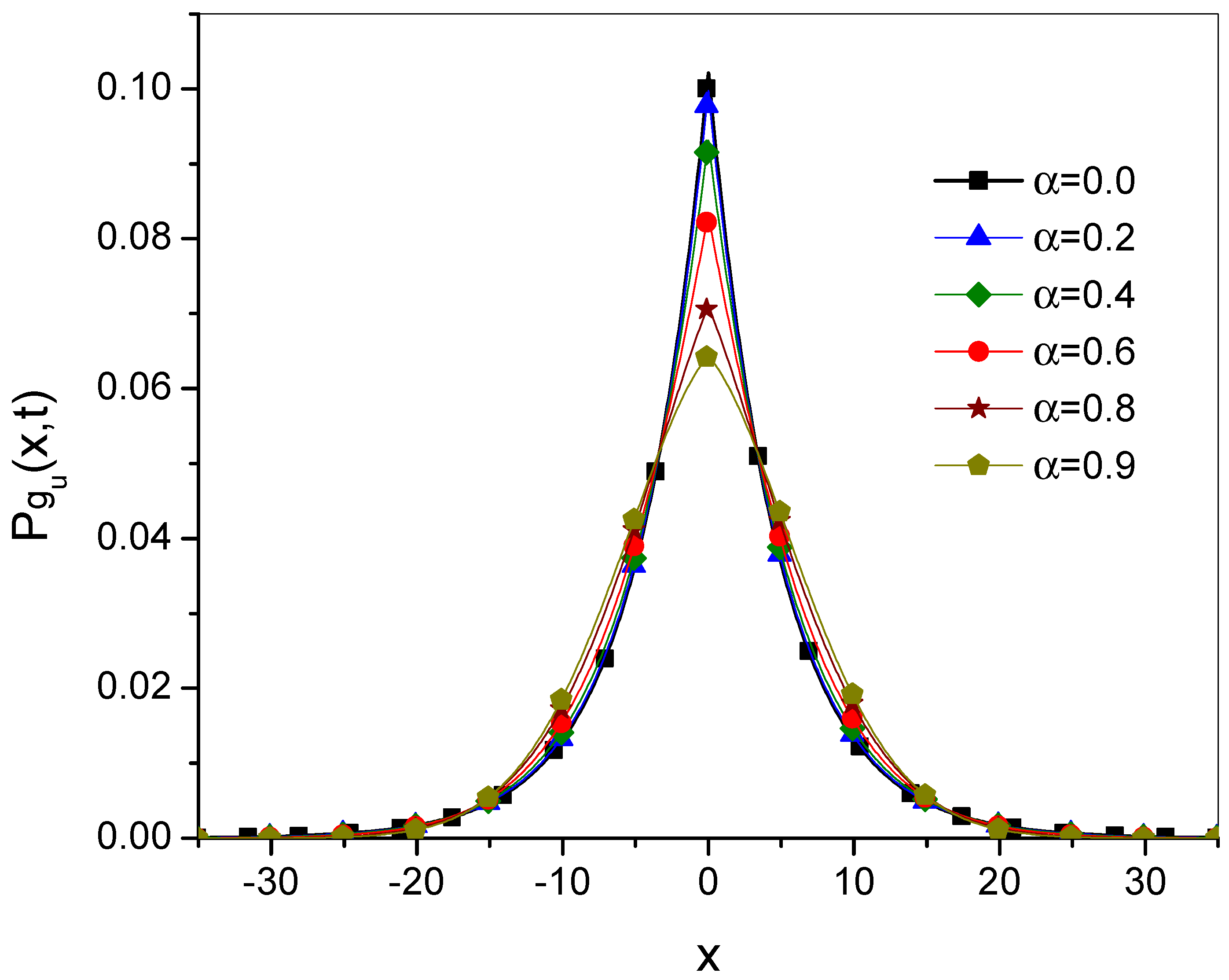
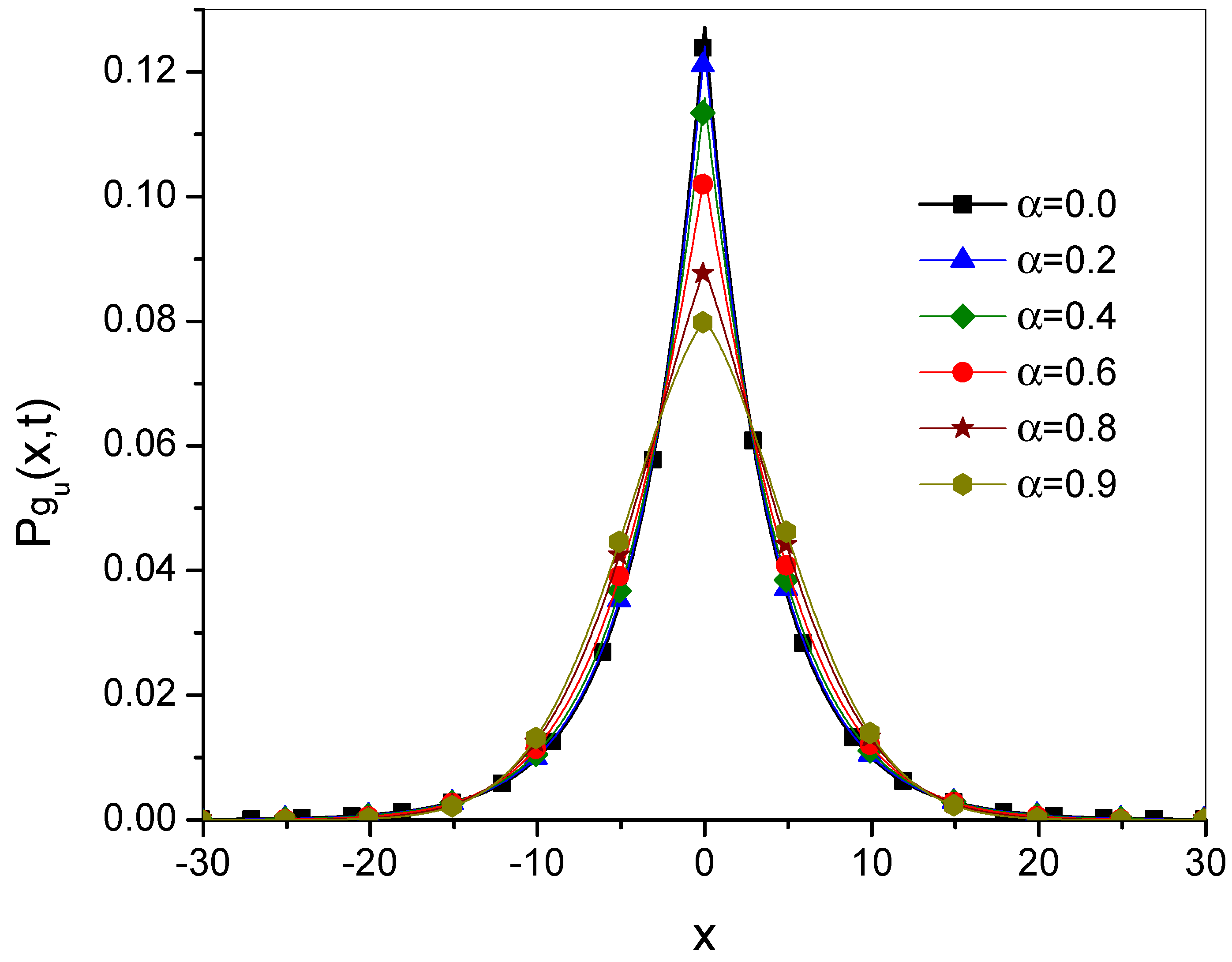
The parameter "accelerates" ultraslow subdiffusion; for larger this effect is greater. The acceleration is evident in the fact that a diffusing molecule is more likely to leave the vicinity of its initial position within a given time for larger values of . However, this acceleration is not large, and the process is still classified as ultraslow diffusion. The plots of the Green’s function Equation (46) for different values of for the processes generated by and are shown in Figure 5 and Figure 6. It can be seen that generates a slightly faster ultraslow diffusion process than .
7. Discussion
The g-subdiffusion equation (47) with the function defined by Equation (44) is useful in modeling ultraslow diffusion (slow subdiffusion) processes in the entire time domain. Ultraslow diffusion is defined here by a slowly varying function generating a slowly varying time evolution of the MSD. The g-subdiffusion equation can also be used to describe the continuous transition between different ultraslow diffusion processes.
The Green’s function for ultraslow diffusion Equation (28) is generated by a slowly varying time-decreasing function such that . Usually, has a stochastic interpretation based on the CTRW model in the long-time limit only [18]. The g-subdiffusion equation and the Green’s function have the stochastic interpretation for , it can be derived from a modified CTRW model [35]. If the function satisfies conditions Equation (45), it generates the function and, consequently, the g-subdiffusion equation describing ultraslow diffusion over entire time domain.
The g-subdiffusion equation can also describe the transition between different diffusion processes. A change in the diffusion process can be caused, for example, by a change in temperature or a change in the density of the diffusing medium. For example, the latter process occurs when a bacterial biofilm reacts to an antibiotic, thereby hindering the diffusion of antibiotic molecules within the biofilm (see the references cited in [15]). In Figure 1, Figure 2 and Figure 3 the gradual transition of the Green’s function from process A to B is shown. It can be seen that the GF for process moves away from the GF for A and is getting closer to the GF for B. In Figure 4, the time evolutions of the MSD for processes A and B and the transition processes and are shown. Note that the process A is faster than the process B (although both are processes much slower than other types of diffusion). Within the model, the transition rate between processes is controlled by the parameter . A larger value of makes the transition process approach the final process more quickly.
The time evolution of MSD has been used to describe the transition process only, not to define the diffusion type. In other words, it describes a transition process that is a time-varying combination of processes A and B. The remark is consistent with the conclusions of articles [41,42] that the time evolution of the MSD cannot always be used as a definition of the diffusion type. When the transition goes from a faster to a slower process, must be a decreasing function over some time interval. Then certainly does not describe a process of spontaneous random walk of a particle.
The order of the time fractional derivative plays an auxiliary role. We note that does not depend on , see Equation (43), while the function does. For the GF Equation (46) coincides with the GF (28) derived in the long-time limit. This fact is consistent with the remark that the ultraslow diffusion process described by the latter GF has a stochastic interpretation when [18]. Then, the distribution of the waiting time for a molecule to jump has a heavy tail that is a slowly varying function, see Equation (26). The g-subdiffusion equation extends the possibility of describing ultraslow diffusion by an equation with a time fractional derivative of order . Larger value of provides a slight acceleration of ultraslow diffusion. The influence of parameter on this process requires further study, including the dependence of the first passage time distribution on both the parameter and the function .
Author Contributions
Conceptualization, T.K. and A.D.; methodology, T.K. and A.D.; validation, T.K. and A.D.; formal analysis, T.K. and A.D.; writing—original draft preparation, T.K. and A.D.; writing—review and editing, T.K. and A.D. All authors have read and agreed to the published version of the manuscript.
Funding
This research received no external funding.
Conflicts of Interest
The authors declare no conflicts of interest.
Abbreviations
The following abbreviations are used in this manuscript:
| MSD | Mean Square Displacement |
| CTRW | Continuous Time Random Walk |
| GF | Green’s Function |
Appendix A
References
- Muñoz-Gil, G. et al. Objective comparison of methods to decode anomalous diffusion. Nature Communications 2021, 12, 6253. [Google Scholar] [CrossRef]
- Oliveira, F.A.; Ferreira, R. M. S.; Lapas, L.C.; Vainstein, M.H. Anomalous Diffusion: A Basic Mechanism for the Evolution of Inhomogeneous Systems. Frontiers in Physics 2019, 7, 00018. [Google Scholar] [CrossRef]
- Metzler, R.; Klafter, J. The random walk’s guide to anomalous diffusion: A fractional dynamics approach. Phys. Rep. 2000, 339, 1–77. [Google Scholar] [CrossRef]
- Metzler, R.; Klafter, J. The restaurant at the end of the random walk: Recent developments in the description of anomalous transport by fractional dynamics. J. Phys. A 2004, 37, R161–R208. [Google Scholar] [CrossRef]
- Klafter, J.; Sokolov, I.M. First Step in Random Walks. From Tools to Applications; Oxford UP: New York, NY, USA, 2011. [Google Scholar]
- Montroll, E.W.; Weiss, G.H. Random walks on lattices II. J. Math. Phys. 1965, 6, 167–181. [Google Scholar] [CrossRef]
- Alcázar-Cano, N.; Delgado-Buscalioni, R. A general phenomenological relation for the subdiffusive exponent of anomalous diffusion in disordered media. Soft Matter 2018, 14, 9937–9949. [Google Scholar] [CrossRef]
- Luo, M.B.; Hua, D.Y. Simulation Study on the Mechanism of Intermediate Subdiffusion of Diffusive Particles in Crowded Systems. ACS Omega 2023, 8, 34188–34195. [Google Scholar] [CrossRef]
- Sokolov, I. M. Models of anomalous diffusion in crowded environments. Soft Matter, 2012, 8, 9043. [Google Scholar] [CrossRef]
- Stauffer, D. , Schulze, C. and Heermann, D.W. Superdiffusion in a Model for Diffusion in a Molecularly Crowded Environment. J. Biol. Phys. 2007, 33, 305–312. [Google Scholar] [CrossRef]
- Mathur, A.; Ghosh, R.; and Nunes-Alves, A. Recent Progress in Modeling and Simulation of Biomolecular Crowding and Condensation Inside Cells. J. Chem. Inf. Model. 2024, 64(24), 9063–9081. [Google Scholar] [CrossRef] [PubMed]
- Bressloff, P. C. and Newby, J. M. Stochastic models of intracellular transport. Rev. Mod. Phys. 2013, 85, 135–196. [Google Scholar] [CrossRef]
- Bouchaud, J.P.; Georgies, A. Anomalous diffusion in disordered media: Statistical mechanisms, models and physical applications. Phys. Rep. 1990, 195, 127–293. [Google Scholar] [CrossRef]
- Kosztołowicz, T.; Dworecki, K.; Mrówczyński, S. How to measure subdiffusion parameters. Phys. Rev. Lett. 2005, 94, 170602. [Google Scholar] [CrossRef]
- Kosztołowicz, T.; Metzler, R. Diffusion of antibiotics through a biofilm in the presence of diffusion and absorption barriers. Phys. Rev. E 2020, 102, 032408. [Google Scholar] [CrossRef]
- Compte, A. Stochastic foundations of fractional dynamics. Phys. Rev. E 1996, 53, 4191–4193. [Google Scholar] [CrossRef]
- Barkai, E.; Metzler, R.; Klafter, J. From continuous time random walks to the fractional Fokker-Planck equation. Phys. Rev. E 2000, 61, 132–138. [Google Scholar] [CrossRef] [PubMed]
- Denisov, S.I. and Kantz, H. Continuous-time random walk with a superheavy-tailed distribution of waiting times. Phys. Rev. E 2011, 83, 041132. [Google Scholar] [CrossRef] [PubMed]
- Denisov, S.I.; Yuste, S.B.; Bystrik Yu, S.; Kantz, H. and Lindenberg K. Asymptotic solutions of decoupled continuous-time random walks with superheavy-tailed waiting time and heavy-tailed jump length distributions. Phys. Rev. E 2011, 84, 061143. [Google Scholar] [CrossRef]
- Godec, A.; Chechkin, A. V.; Barkai, E.; Kantz, H.; Metzler, R. Localisation and universal fluctuations in ultraslow diffusion processes. J. Phys. A: Math. Theor. 2014, 47, 492002. [Google Scholar] [CrossRef]
- Zorbist, B.; Soonsin, V.; Luo, B. P.; Krieger, U. K.; Marcolli, C.; Peter, T.; and Koop, T. Ultra-slow water diffusion in aqueous sucrose glasses. Phys. Chem. Chem. Phys. 2011, 13, 3514. [Google Scholar] [CrossRef] [PubMed]
- Watanabe, H. Relations between anomalous diffusion and fluctuation scaling: the case of ultraslow diffusion and time-scale-independent fluctuation scaling in language. Eur. Phys. J. B 2021, 94, 227. [Google Scholar] [CrossRef]
- Lomholt, M.A.; Lizana, L.; Metzler, R.; and Ambjornsson, T. Microscopic origin of the logarithmic time evolution of aging processes in complex systems. Phys Rev Lett. 2013, 110(20), 208301. [Google Scholar] [CrossRef]
- Meerschaert, M. M.; Scheffler, H. P. Stochastic model for ultraslow diffusion. Stochastic Processes and their Applications 2006, 116, 1215–1235. [Google Scholar] [CrossRef]
- Sinai, Y.G. The limiting behavior of a one-dimensional random walk in a random medium. Theor. Probab. Appl. 1983, 27, 256–268. [Google Scholar] [CrossRef]
- Liang, Y.; Wang, S.; Chen, W.; Zhou, Z.; and Magin, R. L. A Survey of Models of Ultraslow Diffusion in Heterogeneous Materials. ASME. Appl. Mech. Rev. 2019, 71(4), 040802. [Google Scholar] [CrossRef]
- Hu, D.L.; Chen, W.; Liang, Y.J. Inverse Mittag-Leffler stability of structural derivative nonlinear dynamical systems. Chaos, Solitons, Fractals 2019, 123, 304–308. [Google Scholar] [CrossRef]
- Li, C.; Liu, H.; and Xie, X. C. Route of Random Process to Ultraslow Aging Phenomena. Phys. Rev. Lett. 2025, 134, 197102. [Google Scholar] [CrossRef] [PubMed]
- Huang, J. and Zhao, H. Ultraslow diffusion and weak ergodicity breaking in right triangular billiards. Phys. Rev. E 2017, 95, 032209. [Google Scholar] [CrossRef]
- Kosztołowicz, T.; Dutkiewicz, A. Subdiffusion equation with Caputo fractional derivative with respect to another function. Phys. Rev. E 2021, 104, 014118. [Google Scholar] [CrossRef]
- Kosztołowicz, T. Subdiffusion equation with fractional Caputo time derivative with respect to another function in modeling superdiffusion. Entropy 2025, 27, 48. [Google Scholar] [CrossRef] [PubMed]
- Kosztołowicz, T. First-passage time for the g-subdiffusion process of vanishing particles. Phys. Rev. E 2022 106, L022104. [CrossRef] [PubMed]
- Kosztołowicz, T. Subdiffusion equation with fractional Caputo time derivative with respect to another function in modeling transition from ordinary subdiffusion to superdiffusion. Phys. Rev. E 2023, 107, 064103. [Google Scholar] [CrossRef]
- Kosztołowicz, T. and Dutkiewicz, A. Composite subdiffusion equation that describes transient subdiffusion. Phys. Rev. E 2022, 106, 044119. [Google Scholar] [CrossRef]
- Kosztołowicz, T.; Dutkiewicz, A. Stochastic interpretation of g-subdiffusion process. Phys. Rev. E 2021, 104, L042101. [Google Scholar] [CrossRef]
- Kosztołowicz, T.; Dutkiewicz, A.; Lewandowska, K.D. G-Subdiffusion Equation as an Anomalous Diffusion Equation Determined by the Time Evolution of the Mean Square Displacement of a Diffusing Molecule. Entropy 2025, 27, 816. [Google Scholar] [CrossRef]
- Hughes, B. D. Random Walk and Random Environments. Vol. I, Random Walks; Clarendon: Oxford, 1995. [Google Scholar]
- Jarad, F.; Abdeljawad, T. Generalized fractional derivatives and Laplace transform. Discret. Contin. Dyn. Syst. Ser. S 2020, 13, 709–722. [Google Scholar] [CrossRef]
- Jarad, F.; Abdeljawad, T.; Rashid, S.; Hammouch, Z. More properties of the proportional fractional integrals and derivatives of a function with respect to another function. Adv. Differ. Equ. 2020, 2020, 303. [Google Scholar] [CrossRef]
- Almeida, R. A Caputo fractional derivative of a function with respect to another function. Commun. Nonlinear Sci. Numer. Simulat. 2017, 44, 460–481. [Google Scholar] [CrossRef]
- Meroz, Y.; Sokolov, I. M.; and Klafter, J. Unequal twins: probability distributions do not determine everything. Phys. Rev. Lett. 2011, 107, 260601. [Google Scholar] [CrossRef]
- Dybiec, B. and Gudowska-Nowak, E. Discriminating between normal and anomalous random walks. Phys. Rev. E 2009, 80, 061122. [Google Scholar] [CrossRef] [PubMed]
- Kosztołowicz, T. From the solutions of diffusion equation to the solutions of subdiffusive one. J. Phys. A Math. Gen. 2004, 37, 10779–10789. [Google Scholar] [CrossRef]
- Gorenflo, R.; Kilbas, A. A.; Mainardi, F.; and Rogosin, S. V. Mittag-Leffler Functions, Related Topics and Applications; Springer: Berlin, 2014; p. 84. [Google Scholar]
Figure 1.
Plots of the Green’s functions Fequation (46) for the transition from process A to B (solid line with half-filled symbols), for process A (dashed line with empty symbols), and for process B (dotted line with full symbols), for and .
Figure 1.
Plots of the Green’s functions Fequation (46) for the transition from process A to B (solid line with half-filled symbols), for process A (dashed line with empty symbols), and for process B (dotted line with full symbols), for and .
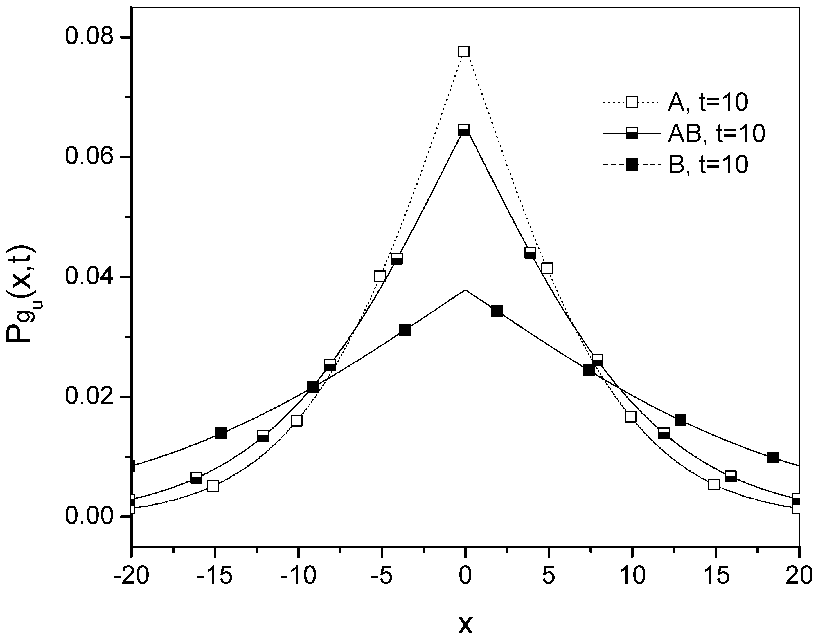
Figure 2.
Similar description as in Figure 1, but for .
Figure 2.
Similar description as in Figure 1, but for .
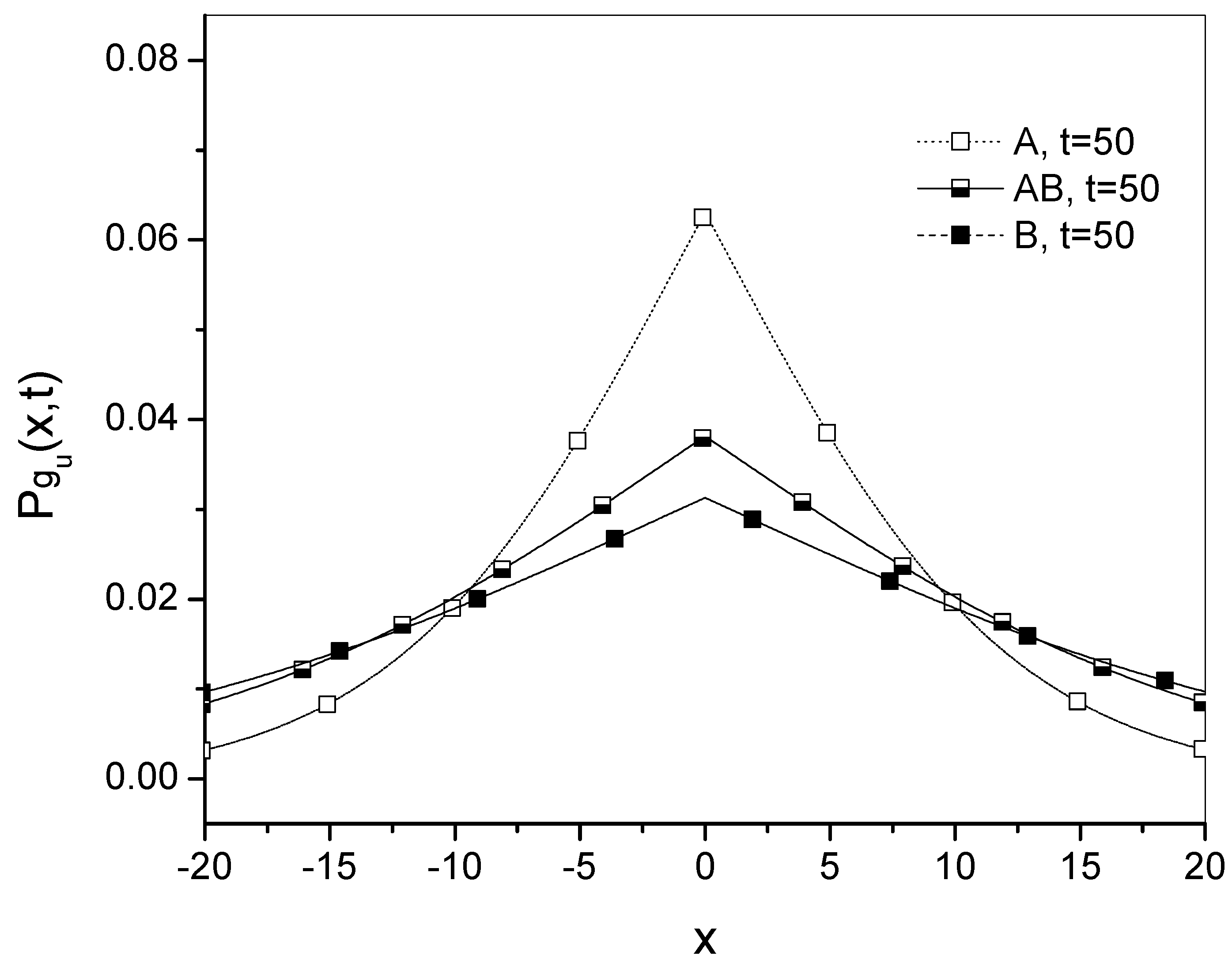
Figure 3.
Similar description as in Figure 1, but for . .
Figure 3.
Similar description as in Figure 1, but for . .
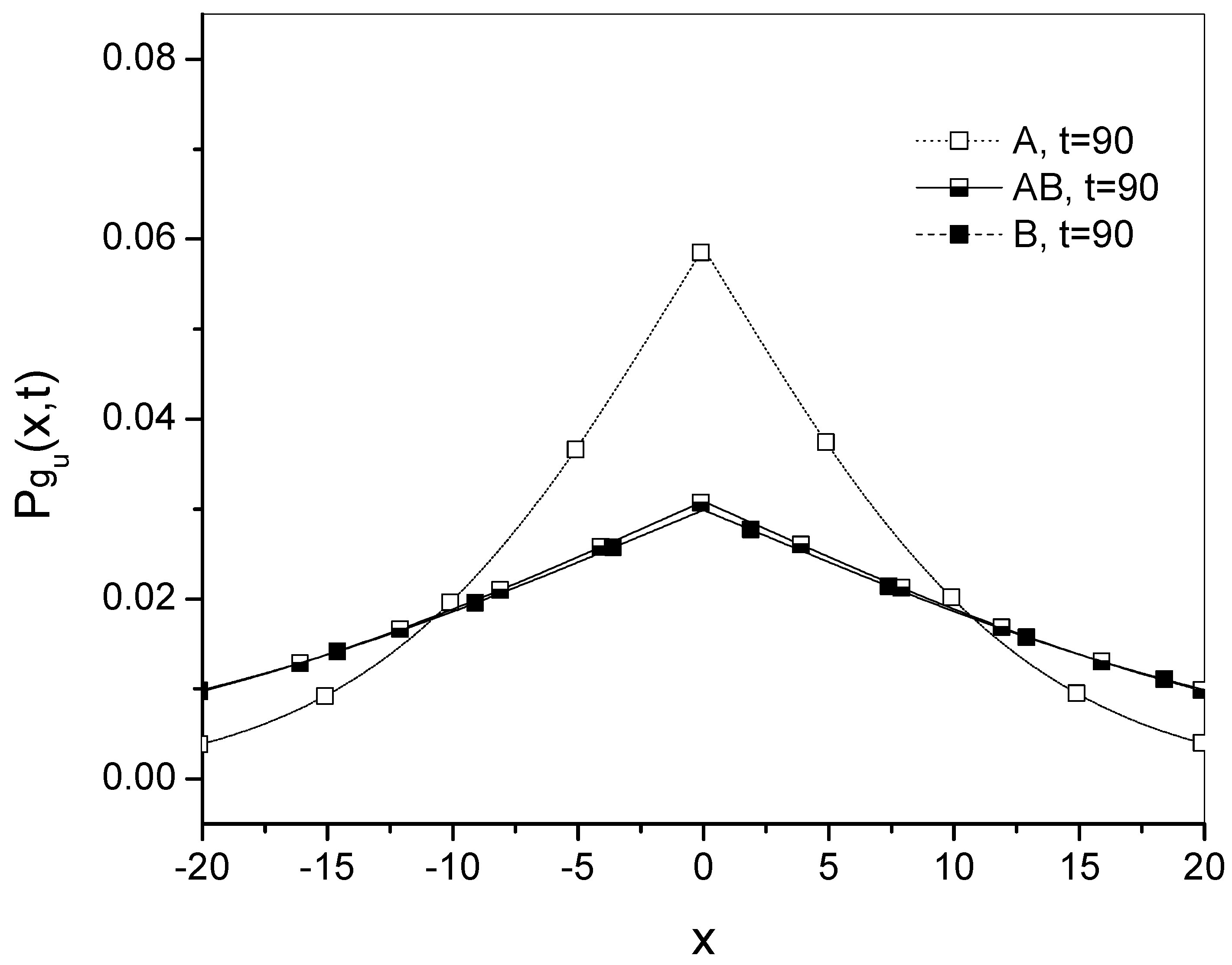
Figure 4.
Plots of the time evolution of MSD Equations (43), (57), and (59) for processes A and B, and for the transition processes from A to B (marked as in the legend) and from B to A (), for different values of the parameter given in the legend.
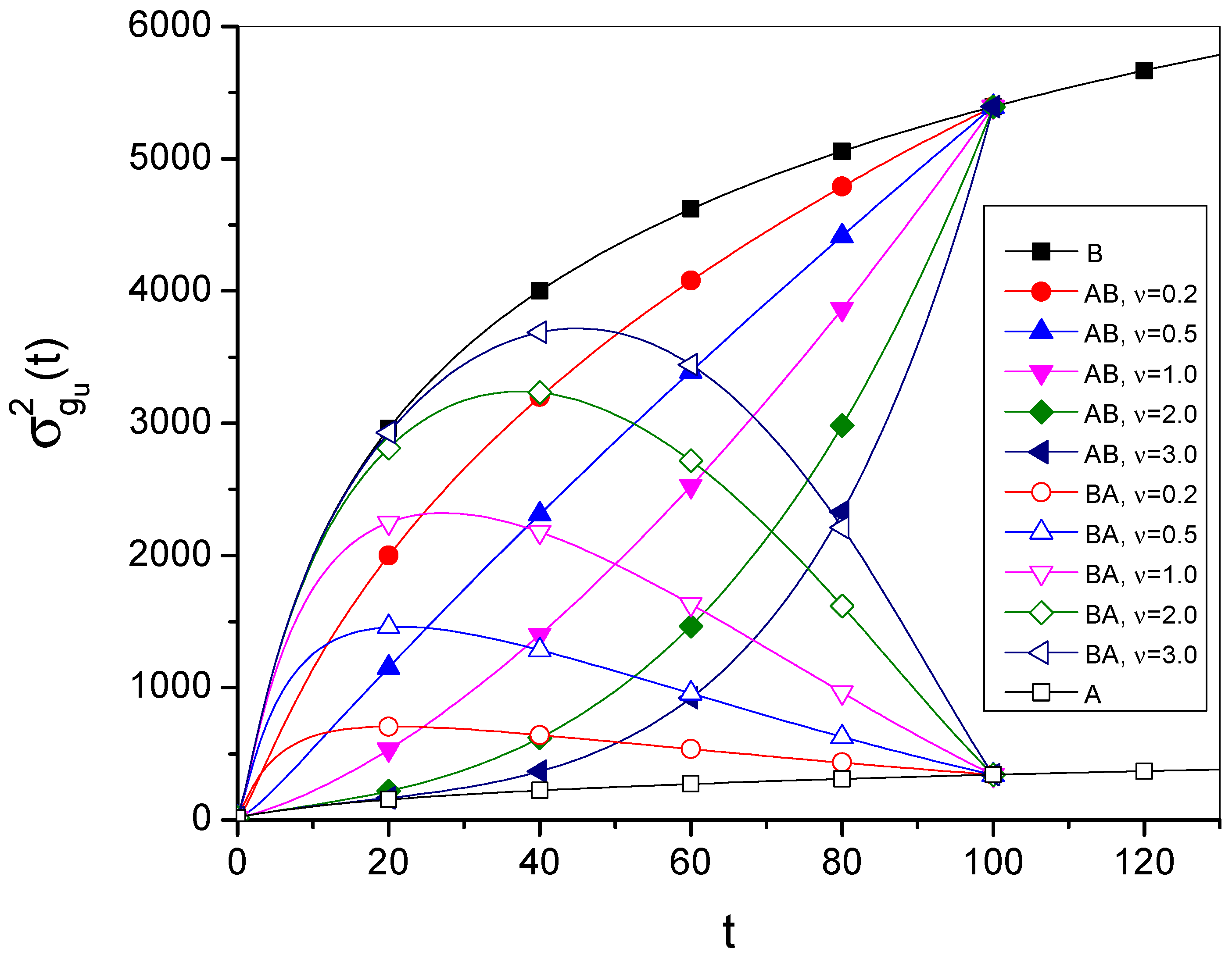
Figure 5.
Plots of the Green’s functions Equation (46) generated by Equation (49) for different values of given in the legend, for .
Disclaimer/Publisher’s Note: The statements, opinions and data contained in all publications are solely those of the individual author(s) and contributor(s) and not of MDPI and/or the editor(s). MDPI and/or the editor(s) disclaim responsibility for any injury to people or property resulting from any ideas, methods, instructions or products referred to in the content. |
© 2025 by the authors. Licensee MDPI, Basel, Switzerland. This article is an open access article distributed under the terms and conditions of the Creative Commons Attribution (CC BY) license (http://creativecommons.org/licenses/by/4.0/).
Copyright: This open access article is published under a Creative Commons CC BY 4.0 license, which permit the free download, distribution, and reuse, provided that the author and preprint are cited in any reuse.


