
Submitted:
29 August 2025
Posted:
02 September 2025
You are already at the latest version
Abstract
Convolution Neural Network (CNN) has excellent performance in various fields such as machine learning, computer vision, and image recognition. With the development of CNNs, huge amount of data in computing and transmission has imposed significant pressure in circuit and architecture design, and RRAM based computing-in-memory (CIM) is one of the promising solutions to alleviate this problem. However, because of the current deviation phenomenon and the resistance on/off ratio (R ratio) issue in RRAM, there is a tradeoff problem between computing accuracy and efficiency for CIM. In this paper, we propose a layer-wise word-line activation strategy to configure the appropriate number of word-line activations for each layer. Based on the observed risk factors, we design a risk index to activated word-lines mapping methodology. Meanwhile, based on the proposed quantization and error calculation methods, we design a CIM simulation framework to simulate the accuracy of CNNs in the inference stage. Experiment results show that for small R ratio, our proposed layer-wise word-line activation methodology reduces up to 63% and 56% of the computation cycles for Cifar-10 and VGG-8, respectively; while the accuracy is decreased by only 0.65% and 0.11%, respectively. On the exploration of increasing the size of R ratio, experiment results show that large R ratio allows our methodology to have a more flexible planning space and better computational efficiency.
Keywords:
CIM
; R ratio
; word-line
; quantization
; CNN
; RRAM
1. Introduction
1.1. Overview
Convolution Neural Networks (CNNs) [1] get excellent performance in many fields such as machine learning, computer vision, and image recognition [2], its brilliant performance depends on massive amount of calculation. In recent years, CNNs architecture becomes much deeper and more complex than before, large amounts of memory access are often the bottleneck that affects the performance and energy consumption of hardware accelerators. Therefore, reducing the access distance between the chip’s external memory and the computing unit or integrating computing power into the memory is the research trend in the architecture design of CNN hardware accelerators [1,2,3]. Among them, methods to reduce the distance between the chip’s external memory and the computing unit include embedded memory (embedded DRAM) or stacking the memory on the computing unit in a three-dimensional manner.
In order to reduce the power consumption and delay caused by data relocation during CNN calculations, in addition to placing on-chip memory close to the computing unit, another way is to use the computing in memory architecture, MAC operations can be integrated into the bit cells of SRAM or non-volatile resistive memories (RRAM). Research results [4] show that the computing in memory architecture can further improve performance and reduce power consumption. Therefore, computing-in-memory (CIM) technique is expected to be the future direction to reduce the amount of external data migration. Some previous works [1,5] have use CIM techniques to successfully reduce large amount of external data migration during CNN computations.
CIM is a technique to reduce data migration in CNNs computation [3]. Its computation architecture and operation method are as illustrated in Figure 1. Input feature map (IFP) input into the CIM array from word-line (WL) in the form of voltage. Weights are stored in memory cells in the form of conductance. The currents produced by memory cells accumulate along the bit-line (BL) and then through the ADC and shifter to convert to computing results.
Computational memory circuits can be roughly divided into two categories: volatile computing-in-memory circuits and non-volatile computing-in-memory circuits. Volatile computing-in-memory circuits are mainly implemented with SRAM; non-volatile computing-in-memory circuits are mainly implemented with RRAM. RRAM has the advantage of short reading latency, low area cost, near zero leakage power [6]. Therefore, it is a good choice for computational memory in the CIM architecture [7]. However, the tiny current produced by the RRAM cells in the high-resistance state may cause an error in the computation result [8]. Ideally, we can activate all word-line at the same time to complete a lot of computation. But in the real world, more word-lines are activated at the same time means more errors are accumulated. Therefore, many works [3,9,10,11] limit the maximum word-lines activated number to avoid error accumulation, and hence has a negative impact on the computation efficiency of CIM.
In this paper, we propose a layer-wise word-line activation strategy to configure the appropriate number of word-line activations for each layer. Based on the observed risk factors, we design a risk index to activated word-lines mapping methodology. Meanwhile, based on the proposed quantization and error calculation methods, we design a CIM simulation framework to simulate the accuracy of CNNs in the inference stage. The proposed methodology improves computation efficiency with only slight accuracy loss.
The rest of this paper is organized as below. In section 2, we describe the background and motivation of layer-wise word-line activation, the effect of current deviation and resistance on/off ratio on computing accuracy and efficiency. Section 3 describe our inference accuracy predictor and layer-wise word-line activation strategy, including risk index, quantization and error calculation methods. In section 4, we show the results of our methodology on Cifar-10 and VGG, analyze and discuss the effect of different R ratio. Finally, we draw conclusions in section 5.
2. Background and Motivation
2.1. Background
2.1.1. Current Deviation
Some features of RRAM may influence the CIM array’s computation result, and the most important one is current deviation. RRAM is consisting of two metal layers and one transition metal oxide layer, and the transition metal oxide layer is between the two metal layers. By applying an external bias to RRAM, an oxidation channel connecting the two metal layers will be formed in the transition metal oxide layer, this state is the low resistance state (LRS). Applying an external bias to cut off the oxidation channel in the transition metal oxide layer is a high resistance state (HRS). By applying different biases, RRAM will transit between the low resistance state and the high resistance state. Since the resistance value is affected by the external bias to affect the formation or interruption of the oxidation channel, so the generated resistance value will not be a constant value.
In the RRAM CIM calculation, it generates a current ILRS through the low-resistance RRAM cell, and generate a current IHRS through the high-resistance RRAM cell. Then the current accumulated by the cells of the same bit line is converted through the analog-to-digital converter and the shifter to get the final calculation result. Ideally, the current generated by the high-resistance RRAM cell should be zero (IHRS=0), which means that only ILRS will accumulate and participate in the subsequent conversion process. However, in reality, the high-resistance RRAM cell will still generate a weak current (IHRS≠0), and the accumulation of multiple IHRS will exceed the tolerance range of the analog-to-digital converter, and causing errors. For the example in Figure 2, there are one HRS and three LRS memory cells on the left most bit line. The ideal situation is accumulating current = 3 x , but the real situation is = + 3 x . The extra may cause an error in the result.
2.1.2. Resistance On/Off Ratio (R Ratio)
The resistance on/off ratio is the ratio of the high-resistance resistance value to the low-resistance resistance value (RHRS / RLRS = R OFF / R ON). Derived from the formula of Figure 3, assuming that the resistance on/off ratio is 10 and the voltage is 1, that is, RHRS : RLRS = 10 : 1. Through the formula I = V /R, we get IHRS : ILRS = 1 : 10, and finally we get 10 x IHRS = ILRS.
Therefore, it can be seen that the larger the resistance on/off ratio, the more IHRS can be tolerated in the calculation (the current deviation part mentioned that IHRS will cause errors). We can reduce the negative factors of current deviation problem by using a large R ratio. However, because a small R ratio has the advantages of low leakage power, low programming cost, high density and high retention time, it is necessary to make a trade-off between large and small R ratios without greatly affecting reliability. By the example of the Cifar-10 network, Figure 4 shows that the larger the R ratio, the larger the AWL (number of WL activated) that can be used.
2.1.3. Number of Activated Word-Lines (AWL)
In CIM calculation, we can choose the number of word-line to be activated at one time. The more WLs activated at one time, the faster the calculation can be completed. However, due to the current deviation problem mentioned above, the more WLs activated, the more IHRS will be generated. In summary, the more WLs activated, the greater the generated error will be. Take Figure 5 as an example, there are three high-resistance cells and one low-resistance cell in the RRAM array on the leftmost column, and the resistance on/off ratio is 2. The example on the left activates one WL at a time, and the example on the right activates all WLs at a time. The calculation on the left requires 4 calculation cycles, and the calculation result is accurate. The calculation on the right only requires 1 calculation cycle, but the calculation result is inaccurate. Obviously, activating one WL at a time can minimize the calculation error, but the calculation time is longer. Activating all WLs at a time can have the fastest calculation efficiency, but the generated calculation error is the largest.
2.2. Motivation
Due to the current deviation problem of the computing memory, the more word-lines are activated at the same time, the more IHRS will be generated, and the greater the calculation error will be. We can reduce the calculation error by controlling the maximum number of word-line activations to be less than the resistance on/off ratio, but from the perspective of computing efficiency, it is not a good thing. This shows that the reliability problem causes the CIM array to not be fully utilized.
By increasing the number of word-line activations, we can effectively increase computing efficiency, but at the same time reduce computing accuracy. For the example of Cifar-10 in Figure 6, when the R ratio is 10, we set the AWL number to be 8 as the benchmark (less than the R ratio so there will be no error). When the AWL is 16, the calculation cycle is reduced by half, and the accuracy rate drops by 5.3%; when the AWL is 64, the calculation cycle only needs one eighth, but the accuracy rate drops to 9.85%. This shows that when the entire network uses the same number of activated word-lines, the scope of increasing calculation efficiency will be very limited because of reliability consideration.
The adjustment of the number of word-line activations in Figure 6 is based on the entire network, that is, all layers use the same number of AWL. However, the number of word-line activations does not have such a big impact on all layers. As shown in Figure 7, we only adjust the AWL of one layer at a time, and the other layers maintain the AWL that will not cause computation errors. From Figure 7, we can see that the second layer of Cifar-10 is the most affected layer by AWL, because this layer has the greatest number of rows in the weight matrix. In contrast, the third layer is less affected by AWL in comparison with the second layer, because it has fewer rows in the weight matrix than the second layer. The first, fourth, and fifth layers are only slightly affected by AWL because the number of rows in the weight matrix is not large in these layers. Through this experiment, we know that the layer with more rows in the weight matrix is more sensitive to the change of AWL. We can use a larger AWL for the layers that are less sensitive to AWL, and a smaller AWL for the layers that are sensitive to AWL.
In addition, current deviation occurs when the weight bit is 0 and the IFM bit is 1. Reducing this situation can also reduce the occurrence of computation errors. Because the highest bit has the greatest impact on the result, we will also use the proportion of 0 in the highest bit to adjust AWL. Figure 8 and Figure 9 show the proportion of weights of 0 in Cifar-10 and VGG-8, respectively.
2.3. Related Works
Although there have been many researches on the computation optimization of CIM [3,4,5,6,7,8,9,10,11,12], only a few of them discuss the issue of activated word-lines number, and its effect on computing accuracy and computing efficiency. In our study, some works for RRAM-based CIM limit the maximum number of concurrently activated word-lines. For example, manuscripts [9,10] show that only 9 out of 256 word-lines are activated at the same time, and manuscript [11] shows that only 16 out of 512 word-lines are activated at the same time.
Manuscript [3] is the seldom one that exploring the AWL problem of CIM on inference DNN accelerators. Their method is to first adjust the number of word-line activations in layers for experiments (error caused by only one layer), and record the information of accuracy drop. Then use the greedy algorithm to select the layer and word-line activation number that causes the smallest error and then conduct experiments to evaluate the accuracy. Only one layer is selected for adjustment in each round until the accuracy drops beyond the set threshold. However, this method requires multiple experiments to determine the AWL number for each layer, and they do not consider the proportion of 0 in weight bits as described above.
Except the computation optimization methodology, there have also been some developed memristor-based DNN simulation frameworks [13,14,15,16,17,18,19,20,21,22,23,24] to evaluate accuracy and efficiency. NeuroSIM [17,18] is a circuit-level simulation platform that can be used to assess accelerator area, power consumption, and performance, but its architecture is not easily modified to meet our needs. MNSIM [19] offers a hierarchical modular design approach, allowing for area, power consumption, and inference accuracy assessments. However, MNSIM assesses accuracy under worst-case and average scenarios, resulting in lower accuracy than actual conditions. MemTorch [20,21] and AIHWKit [22] can support multiple types of layers and use a modular approach for hardware design. DL-RSIM [23] can simulate various factors that affect computational memory reliability. These simulation frameworks have their own areas of expertise, but they do not meet the needs of layer-wise AWL architecture. Therefore, development of a layer-wise DNN framework based on RRAM is necessary.
Due to these issues, in this paper, we propose a methodology to config suitable AWL size for each layer according to features of the neural network (length of weight matrix, layer type, etc.), R ratio, and others. While increasing computation efficiency, we also consider the maintenance of accuracy. In addition, we also developed a layer-wise CIM simulation framework to evaluate the accuracy and efficiency of our proposed methodology in the inference stage.
3. Proposed Framework and Methodology
3.1. Inference Accuracy Predictor
We designed a CIM simulation tool: inference accuracy predictor that simulates the CIM operation in the inference stage and was developed in Windows 10, Anaconda 23.3.1 and Python 3.10.9. The tool simulates the error that appeared from the CIM operation with the hardware restriction (R ratio, ADC precision, and AWL) given by the user, then it gives the accuracy report.
The architecture of inference accuracy predictor is shown in Figure 10. Before we use inference accuracy predictor, we need to train and keep the weight by Keras. Then weights, model, test dataset, and hardware constraints are fed into inference accuracy predictor. Weights and model are used to build the inference model, and test dataset is input of the inference model. In convolution layers and fully connected layers, weights and IFMs are quantized according to ADC precision. Then they are fed into the CIM array, calculated in batches according to AWL. Finally, the output current is converted into the value by ADC according to R ratio and ADC precision. After the inference phase, inference accuracy predictor gives the accuracy result of the impact of AWL and ADC precision.
3.2. Quantization Method
In CNN computations, weights and IFMs are typically stored as floating-point numbers. To conserve hardware resources and increase computational efficiency, the original values are typically quantized to reduce the number of bits required to represent them.
In the proposed inference accuracy predictor, we use linear transformation method to convert weight and IFMs to the specified interval. For the example of 8-bit quantization, formula (1) shows that since the weight range is [-1, 1], the weight is converted from a floating-point number between [-1, 1] to an integer between [-128, 127]. Because the input feature map doesn’t have a clear range, we use the maximum and minimum values as the range boundaries for conversion, that is, convert [IFM minimum, IFM maximum] to [0, 255] as shown in formula (2).
In the convolutional computation, we add 128 to the converted weight, so the weight conversion range becomes [0, 255]. The additional 128 will be deducted after the calculation is completed and will not affect the result. As shown in Figure 11, we can simply deduct Σ(Ai∗128) after the calculation without affecting the computing result. This allows us to avoid the need of considering the positive and negative signs during the calculation process.
Figure 12 is the weight distribution of Cifar-10. We can observe that the weight distribution exhibits a normal distribution, with most weights concentrated around 0 (the center), and the weight distribution decreasing towards either side. Therefore, during quantization, we narrow the weight range from [-1, 1] to [-0.8, 0.8]. Weights greater than 0.8 are stored as 0.8, and weights less than -0.8 are stored as -0.8. By quantizing within a narrow range, we can create greater disparity between weights in the densely populated middle range, thereby improving the accuracy. Formula (3) is the final weight quantification equation.
3.3. Error Calculation
To calculate the current error, we need to compute it in bits, but this is far inefficient. So, we compute the correct result and the error current separately to speed up the simulation as shown in Figure 13. The correct result is calculated as in Keras, multiplying the weights and the IFM and accumulating them. The error current is calculated by accumulating the number along the BL with a weight of 0 and an IFM of 1. It is calculated in batches according to the AWL, converted into a value, then added to the correct result and stored. We use this approach to avoid performing accurate numerical calculations at the bit level, and to discard the numerical conversion of the current of the high-configuration computing memory unit that does not cause errors.
3.4. Layer-wise AWL Decision Methodology
In our research, several factors influence the AWL size selection. The first is the size of the R ratio. The larger the R ratio, the greater the error current that can be tolerated in the calculation. The second is the type of neural network layer. Convolutional layers require higher accuracy because they are typically ranked earlier. If accuracy is lost early in the computation, subsequent layers are more likely to experience worse accuracy. Fully connected layers are typically ranked later, so a larger AWL can be used for these layers. The third is the number of expanded weight rows. This represents the number of dot products that need to be accumulated for one output pixel. A larger value indicates more rows need to be accumulated, which in turn means a greater potential for accumulated current deviation. The last is the proportion of 0 in the highest-weighted bit. A higher proportion of 0 indicates a higher number of high-configuration computing memory cells, which increases the probability of current error. The above four observations are collectively called risk factors.
Table 1 shows the risk factors and their impact value on risk index. We calculate the risk index layer by layer according to the characteristics of each layer. Initially the risk index of each layer is 0, the final risk index of a layer is obtained by summing its corresponding impact values. Among the risk factors, except matrix row, we consider all other risk factors to be equally important, and the impact values of them are ±1 as shown in Table 1. Therefore, for a convolution layer, we increase its risk index by one, while for a FC layer we decrease its risk index by one; if the ratio of 0 in MSB is large enough in a layer, we also increase its risk index by one; if the R ratio is small, we will increase the risk index of all layers by one, and vice versa. Finally, we observe that the size span of matrix row is large, so we calculate its impact value by .
For each layer, the selected AWL size is based on its risk index. The larger the risk index, the greater the error that may occur, so a small AWL should be used to reduce the error. On the contrary, a large AWL can be used for layers with smaller risk index. The corresponding mapping is as shown in Table 2.
4. Evaluation Results
4.1. Experiment Setup
We verify our methodology on Cifar-10 [25] and VGG-8 [26], and use the proposed RRAM accuracy predictor to simulate accuracy and efficiency. The CIM hardware settings are shown in Table 3. We use a 512*512 CIM array based on RRAM, each RRAM cell represents one bit data. We analyze the number of word-line layer-wise activations and computation efficiency under different R ratios.
The selection of R ratio has an obvious impact on the generated current error. In manuscript [3], they use the R ratio size of 15, 25, and 35 to simulate the number of word-line activations. In this paper, we firstly use a small R ratio to discuss the effect of number of word-line activations, so set the R ratio sizes to be 10, 15, and 20 in the experiments.
4.1.1. Cifar-10
Table 4 shows the architecture of Cifar-10, matrix row is the number of rows of the weight matrix, its formula is , and matrix col. is Depth. Table 5 lists the risk factors of each layer based on the Cifar-10 architecture, we calculate the risk index of each layer based on the impact values of the risk factors in Table 1, the results are shown in Table 6.
Take the second layer with R ratio 15 as an example, the risk factors of the second layer including (1) layer type is convolution, (2) matrix ow (R) >= 256, (3) ratio of 0 in MSB >= 55%. Therefore, the risk index is (1)+(2)+(3) = 1+⌊log2800−7⌋+1=4. After calculating the risk index and referring to Table 2, we can get that the AWL size of the second layer with R ratio 15 is 16. The AWL size of the first layer with R ratio 15 is 32 instead of 64 as shown in Table 6, this is because that the matrix row of the first layer is only 27, AWL size of 32 is enough to fully calculated in one go. The same reason is also applied to the AWL size of the first layer with R ratio 20, and the AWL size of the last two layers with R ratio 15 and 20, respectively.
4.1.2. VGG-8
Table 7, Table 8 and Table 9 show the VGG-8 architecture, risk factors, risk index, and AWL of each layer. Taking layer 7 with R ratio of 15 as an example, the risk factors including (1) matrix row (R) >= 256, (2) ratio of 0 in MSB >= 55%, (3) layer type is fully connected and R ratio > 10. The risk index is calculated as (1)+(2)+(3) = . Referring to Table 2, we see that the AWL size of layer 7 is 16.
4.2. Analysis of Accuracy and Efficiency for Small R Ratio
4.2.1. Results
The AWL and accuracy of each layer of Cifar-10 are shown in Table 10. Since we mainly discuss the impact of AWL on accuracy, we use the quantified accuracy as the benchmark which is 59%. By using our methodology, the accuracy is reduced by 3.35% when R ratio is 10; when R ratio is 15, the accuracy is reduced by 1.8%; when R ratio is 20, the accuracy is reduced by 0.65%.
The computation efficiency is shown in Table 11. We set the AWL of all layers to be 8 as the benchmark (no error) for comparison. By using our methodology, when R ratio is 10, the cycles required for calculation is reduced by 9%; when R ratio is 15, the cycles is reduced by 54%; when R ratio is 20, the cycles is reduced by 63%.
The AWL and accuracy of each layer of VGG-8 are shown in Table 12, we also use the quantified accuracy as the benchmark which is 64.9%. By using our methodology, the accuracy is reduced by 2.9% when R ratio is 10; when R ratio is 15, the accuracy is reduced by 1%; when R ratio is 20, the accuracy is reduced by 0.11%.
The computation efficiency is shown in Table 13. We set the AWL of all layers to be 8 as the benchmark (no error) for comparison. By using our methodology, when R ratio is 10, the cycles is reduced by 5%; when R ratio is 15, the cycles is reduced by 52%; when R ratio is 20, the cycles is reduced by 56%.
4.2.2. Discussion
Experiments on Cifar-10 and VGG-8 have verified that our methodology can effectively reduce the cycles required for computation without losing too much accuracy. When R ratio = 20, our methodology performs best in terms of accuracy and computational efficiency. This is because that the larger the R ratio, the more current deviations can be tolerated. Therefore, when R ratio = 20, we can use a larger AWL. Compared with R ratio = 10, we can more flexibly plan the AWL size of each layer. These results show that the methodology we proposed to plan AWL layer by layer performs better in terms of computational efficiency and maintains a certain level of accuracy compared to the methodology that using the same AWL size for all layers.
4.3. Exploration on Large R Rario and AWL Size
4.3.1. Risk Index and AWL Mapping
In order to demonstrate that the methodology proposed in this paper can also effectively improve computing efficiency under large R ratio, we refer to manuscript [3] and verify our methodology on the Cifar-10 architecture with R ratio 25 and 35, Table 14 lists the corresponding risk index. Because the larger the R ratio, the larger the minimal AWL size can be used. Therefore, for R ratio 25 and 35, the minimal AWL size can be modified from 16 to 32 or even larger. In addition to the original risk index and AWL mapping for small R ratio (min. AWL = 16), Table 15 shows the mapping of risk index and different min. AWL for large R ratio.
4.3.2. Results
Table 16 and Table 17 show the AWL size for each layer of Cifar-10, respectively, when R ratios are 25 and 35, and when the minimum AWL value ranges from 16 to 256. The accuracy and computational efficiency gains achieved with these AWL configurations are also shown. With a minimum AWL of 128, we speculate that the slight increase in accuracy is due to the fact that the error introduced by this configuration just causes some data that the original model had previously misjudged to be correct. These two tables show a significant drop in accuracy only at a minimum AWL of 256. Therefore, for R ratios of 25 and 35, increasing the minimum AWL value from 16 to 64 or 128 yields the best results.
From these two tables, we know that increasing the size of R ratio allows our methodology to use a larger AWL and achieve better computation efficiency. At the same time, we know that increasing the size of R ratio can improve the problem of declining accuracy. However, manuscript [23] mentioned that the current range of R ratio mostly falls between 10 and 50, so this problem cannot be solved by infinitely increasing R ratio. Furthermore, increasing the R ratio size will also increase the hardware area, which is a burden for devices with limited size. For our methodology, increasing the size of R ratio to solve the problem of declining accuracy is not a blow but a help. Increasing the size of R ratio allows our methodology to have a more flexible planning space and better computational efficiency.
Because the two experimental results with a Min AWL of 128 in Table 16 and Table 17 both show a slight increase in accuracy, we also try to increase the AWL size used with a small R ratio for exploration. Table 18 and Table 19 are the experimental results with R ratios of 10, 15, and 20 and Min AWLs of 32 and 64. From these two tables, we can see that the accuracy also shows a slight increase when R ratio = 20 and Min AWL is 64.
4.3.3. Discussion
We plot the accuracy rates in Table 16 and Table 17 as a function of the amount of input data in line graphs (Figure 14 and Figure 15). The baseline represents the accuracy change without error. The blue, red, yellow, and green lines in both figures almost overlap. The orange lines represent the accuracy change with a Min AWL of 128. The orange line in Figure 14 initially shows a higher accuracy than the blue line representing the baseline, the orange line in Figure 15 starts slightly lower than the baseline, then gradually converges to the baseline in both figures.
Errors in calculations can cause the model to identify previously correct results incorrectly, or incorrect results correctly. Therefore, accuracy doesn’t simply decrease or increase. From Figure 14, we can see that the initial orange line has a higher accuracy than the baseline, this indicates that the errors in the early stages just caused a larger number of incorrect results to become correct, resulting in a higher accuracy than the baseline. As the orange line gradually approaches the baseline, it indicates a continuous decrease in accuracy. Therefore, we can infer that errors in the later stages caused a larger number of correct results to become incorrect, leading to a continuous decrease in accuracy. As previously mentioned, a smaller R ratio results in greater error. An R ratio of 25 will produce a larger error than an R ratio of 35. Therefore, under the same AWL plan, an R ratio of 25 will cause a more drastic change in accuracy than an R ratio of 35.
5. Conclusions
This paper proposes a CIM simulation platform based on inference-phase simulation and accuracy evaluation, considering factors influencing accuracy, such as AWL and R ratio. We also propose a layer-by-layer word-line activation method that calculates a risk index based on the network type, weight matrix size, R ratio, and the proportion of the highest bit 0 at each layer to determine the required AWL size for each layer.
For small R ratio, experimental results show that our method reduces the number of computational cycles required for Cifar-10 by up to 63%, while simultaneously decreasing accuracy by 0.65%. For VGG-8, the number of computational cycles required is reduced by up to 56%, while decreasing accuracy by 0.11%. These results demonstrate that our proposed method can reduce computational costs while maintaining relatively stable accuracy. On the exploration of large R ratio, increasing the size of R ratio allows our methodology to have a more flexible planning space and better computational efficiency.
Author Contributions
Conceptualization and methodology, W.-K.C. and S.-Y.P.; validation and formal analysis, S.-Y.P.; investigation, W.-K.C. and S.-Y.P.; writing—original draft preparation, W.-K.C. and S.-Y.P.; writing—review and editing, W.-K.C. and S.-H.H; supervision, S.-H.H. All authors have read and agreed to the published version of the manuscript.
Funding
This work was supported in part by the National Science and Technology Council, Taiwan, under grant number 111-2221-E-033-042 and grant number 113-2221-E-033-030.
Data Availability Statement
The data used to support the findings of this study are included in
this paper.
Conflicts of Interest
The authors declare no conflict of interest.
References
- Lecun, Y.; Bengio, Y.; Hinton, G. Deep learning. Nature 2015, 521, 436–444. [Google Scholar] [CrossRef] [PubMed]
- Krizhevsky, A.; Sutskever, I.; Hinton, G. ImageNet Classification with Deep Convolutional Neural Networks. In Proceedings of the Neural Information and Processing Systems (NIPS), Lake Tahoe, NV, USA, 3-8 December 2012. [Google Scholar]
- Park, Y.; Lee, S.Y.; Shin, H.; Heo, J.; Ham, T.J.; Lee, J.W. Unlocking Wordline-level Parallelism for Fast Inference on RRAM-based DNN Accelerator. In Proceedings of the 39th International Conference on Computer-Aided Design (ICCAD), San Diego, CA, USA, 2-5 November 2020. [Google Scholar]
- Verma, N.; Jia, H.; Valavi, H.; Tang, Y.; Ozatay, M.; Chen, L.Y.; Zhang, B.; Deaville, P. In-Memory Computing: Advances and prospects. IEEE Solid-State Circuits Magazines 2019, 11, 43–55. [Google Scholar] [CrossRef]
- Shafiee, A.; Nag, A.; Muralimanohar, N.; Balasubramonian, R.; Strachan, J.P.; Hu, M.; Williams, R.S.; Srikumar, V. ISAAC: A Convolutional Neural Network Accelerator with In-Situ Analog Arithmetic in Crossbars. In Proceedings of the 43rd International Symposium on Computer Architecture (ISCA), Seoul, Korea, 18-22 June 2016. [Google Scholar]
- Wong, H.S.P.; Lee, H.Y.; Yu, S.; Chen, Y.S.; Wu, Y.; Chen, P.S.; Lee, B.; Chen, F.T.; Tsai, M.J. Metal–Oxide RRAM. Proceedings of the IEEE 2012, 100, 1951–1970. [Google Scholar] [CrossRef]
- Hu, M.; Strachan, J.P.; Li, Z.; Grafals, E.M.; Davila, N.; Graves, C.; Lam, S.; Ge, N.; Yang, J.J.; Williams, R.S. Dot-product engine for neuromorphic computing: Programming 1T1M crossbar to accelerate matrix-vector multiplication. In Proceedings of the 53rd ACM/EDAC/IEEE Design Automation Conference (DAC), Austin, TX, USA, 5-9 June 2016. [Google Scholar]
- Feinberg, B.; Wang, S.; Ipek, E. Making Memristive Neural Network Accelerators Reliable. In Proceedings of the IEEE International Symposium on High Performance Computer Architecture (HPCA), Vienna, Austria, 24-28 February 2018. [Google Scholar]
- Chen, W.H.; Li, K.X.; Lin, W.Y.; Hsu, K.H.; Li, P.Y.; Yang, C.H.; Xue, C.X.; Yang, E.Y.; Chen, Y.K.; Chang, Y.S.; Hsu, T.H.; King, Y.C.; Lin, C.J.; Liu, R.S.; Hsieh, C.C.; Tang, K.T.; Chang, M.F. A 65nm 1Mb nonvolatile computing-in-memory ReRAM macro with sub-16ns multiply-and-accumulate for binary DNN AI edge processors. In Proceedings of the IEEE International Solid-State Circuits Conference (ISSCC), San Francisco, CA, USA, 11-15 February 2018. [Google Scholar]
- Xue, C.X.; Chen, W.H.; Liu, J.S.; Li, J.F.; Lin, W.Y.; Lin, W.E.; Wang, J.H.; Wei, W.C.; Chang, T.W.; Chang, T.C.; Huang, T.Y.; Kao, H.Y.; Wei, S.Y.; Chiu, Y.C.; Lee, C.Y.; Lo, C.C.; King, Y.C.; Lin, C.J.; Liu, R.S.; Hsieh, C.C.; Tang, K.T.; Chang, M.F. A 1Mb Multibit ReRAM Computing-In-Memory Macro with 14.6ns Parallel MAC Computing Time for CNN Based AI Edge Processors. In Proceedings of the IEEE International Solid-State Circuits Conference (ISSCC), San Francisco, CA, USA, 17-21 February 2019. [Google Scholar]
- Xue, C.X.; Huang, T.Y.; Liu, J.S.; Chang, T.W.; Kao, H.Y.; J. Wang, J.H.; Liu, T.W.; Wei, S.Y.; Huang, S.P.; Wei, W.C.; Chen, Y.R.; Hsu, T.H.; Chen, Y.K.; Lo, Y.C.; Wen, T.H.; Lo, C.C.; Liu, R.S.; Hsieh, C.C.; Tang, K.T.; Chang, M.F. A 22nm 2Mb ReRAM Compute-in-Memory Macro with 121–28TOPS/W for Multibit MAC Computing for Tiny AI Edge Devices. In Proceedings of the IEEE International Solid-State Circuits Conference (ISSCC), San Francisco, CA, USA, 16-20 February 2020.
- Chi, P.; Li, S.; Qi, Z.; Gu, P.; Xu, C.; Zhang, T.; Zhao, J.; Liu, Y.; Wang, Y.; Xie, Y. PRIME: A Novel Processing-In-Memory Architecture for Neural Network Computation in ReRAM-based Main Memory. In Proceedings of the 43rd International Symposium on Computer Architecture (ISCA), Seoul, Korea, 18-22 June 2016. [Google Scholar]
- Imani, M.; Samragh, M.; Kim, Y.; Gupta, S.; Koushanfar, F.; Rosing, T. RAPIDNN: In-Memory Deep Neural Network Acceleration Framework. arXiv:1806.05794, 2018.
- Ankit, A.; Hajj, I.E.; Chalamalasetti, S.R.; Ndu, G.; Foltin, M.; Williams, R.S.; Faraboschi, P.; Hwu, W.; Strachan, J.P.; Roy, K.; Milojicic, D.S. PUMA: A Programmable Ultra-efficient Memristor-based Accelerator for Machine Learning Inference. arXiv:1901.10351, 2019.
- Ma, X.; Yuan, G.; Lin, S.; Ding, C.; Yu, F.; Liu, T.; Wen, W.; Chen, X.; Wang, Y. Tiny but Accurate: A Pruned, Quantized and Optimized Memristor Crossbar Framework for Ultra Efficient DNN Implementation. arXiv:1908.10017, 2019.
- Yuan, G.; Ma, X.; Ding, C.; Lin, S.; Zhang, T.; Jalali, Z.S.; Zhao, Y.; Jiang, L.; Soundarajan, S.; Wang, Y. An Ultra-Efficient Memristor-Based DNN Framework with Structured Weight Pruning and Quantization Using ADMM. arXiv:1908.11691, 2019.
- Peng, X.; Huang, S.; Luo, Y.; Sun, X.; Yu, S. DNN+NeuroSim: An End-to-End Benchmarking Framework for Compute-in-Memory Accelerators with Versatile Device Technologies. In Proceedings of the IEEE International Electron Devices Meeting (IEDM), San Francisco, CA, USA, 7-11 December 2019. [Google Scholar]
- Peng, X.; Huang, S.; Jiang, H.; Lu, A.; Yu, S. DNN+NeuroSim V2.0: An End-to-End Benchmarking Framework for Compute-in-Memory Accelerators for On-Chip Training. IEEE Transactions on Computer-Aided Design of Integrated Circuits and Systems 2021, 40, 2306–2319. [Google Scholar] [CrossRef]
- Xia, L.; Li, B.; Tang, T.; Gu, P.; Yin, X.; Huangfu, W.; Chen, P.Y.; Yu, S.; Cao, Y.; Wang, Y.; Xie, Y.; Yang, H. MNSIM: Simulation platform for memristor-based neuromorphic computing system. In Proceedings of the Design, Automation & Test in Europe Conference & Exhibition (DATE), Dresden, Germany, 14-18 March 2016. [Google Scholar]
- Lammie, C.; Azghadi, M.R. MemTorch: A Simulation Framework for Deep Memristive Cross-Bar Architectures. In Proceedings of the IEEE International Symposium on Circuits and Systems (ISCAS), Seville, Spain, 12-14 October 2020. [Google Scholar]
- Lammie, C.; Xiang, W.; Linares-Barranco, B.; Azghadi, M.R. MemTorch: An open-source simulation framework for memristive deep learning systems. Neurocomputing 2022, 485, 124–133. [Google Scholar] [CrossRef]
- Rasch, M.J.; Moreda, D.; Gokmen, T.; Gallo, M.L.; Carta, F.; Goldberg, C.; Maghraoui, K.E.; Sebastian, A.; Narayanan, V. A Flexible and Fast PyTorch Toolkit for Simulating Training and Inference on Analog Crossbar Arrays. In Proceedings of the 3rd IEEE International Conference on Artificial Intelligence Circuits and Systems (AICAS), Washington, DC, USA, 6-9 June 2021. [Google Scholar]
- Lin, M.Y.; Cheng, H.Y.; Lin, W.T; Yang, T.H.; Tseng, I.C.; Yang, C.L.; Hu, H.W.; Chang, H.S.; Li, H.P.; Chang, M.F. DL-RSIM: A Simulation Framework to Enable Reliable ReRAM-based Accelerators for Deep Learning. In Proceedings of the 37th International Conference on Computer-Aided Design (ICCAD), San Diego, CA, 5-8 November 2018. [Google Scholar]
- Lammie, C.; Xiang, W.; Azghadi, M.R. Modeling and simulating in-memory memristive deep learning systems: An overview of current efforts. Array 2022, 13, Article–100116. [Google Scholar] [CrossRef]
- Shahrestani, A. Classifying CIFAR-10 using a simple CNN. https://medium.com/analytics-vidhya/classifying-cifar-10-using-a-simple-cnn-4e9a6dd7600b.
- Simonyan, K.; Zisserman, A. Very Deep Convolutional Networks for Large-Scale Image Recognition. arXiv:1409.1556, 2014.
Figure 1.
CIM computing architecture.
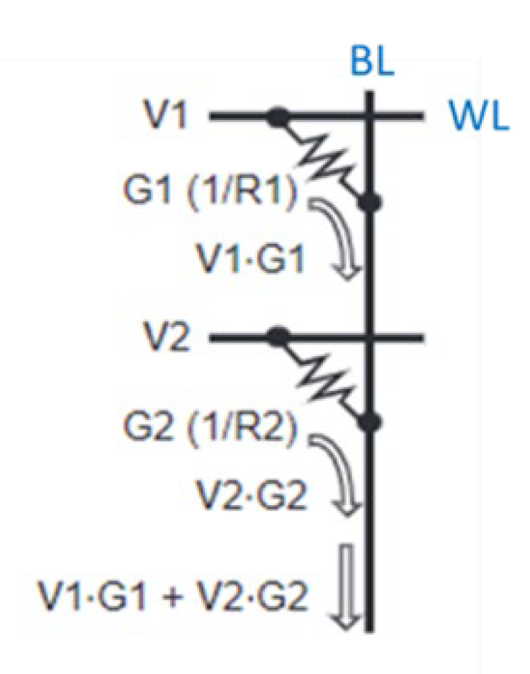
Figure 2.
Example of current deviation.
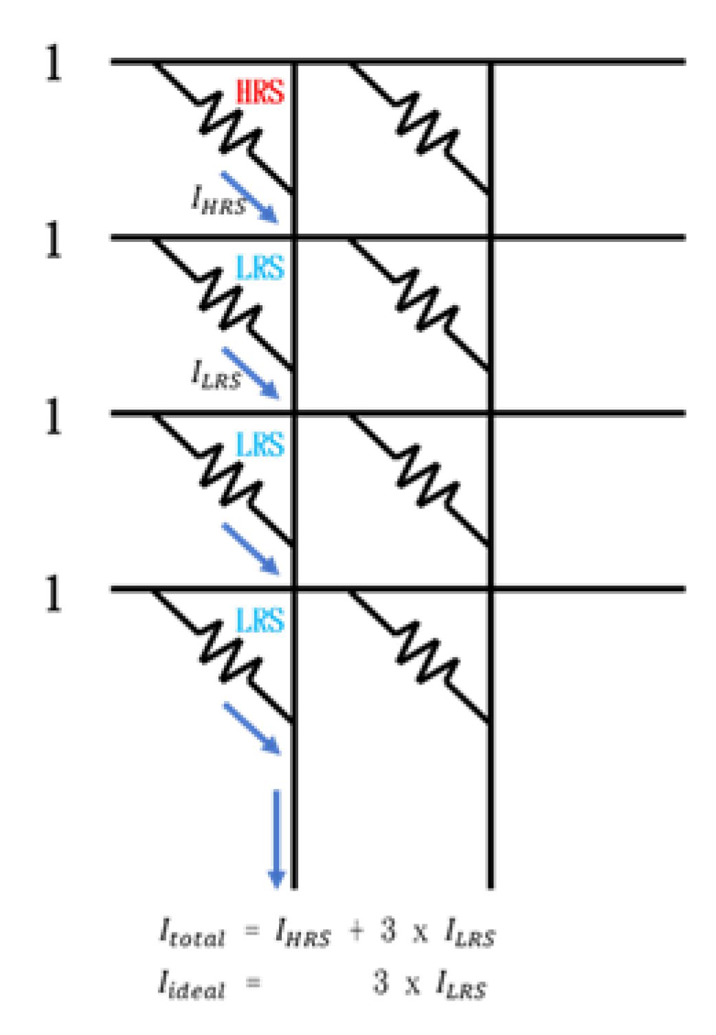
Figure 3.
Example of R ratio and IHRS vs. ILRS.
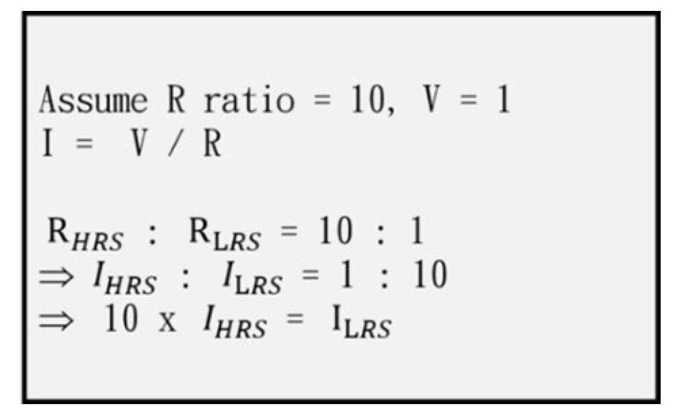
Figure 4.
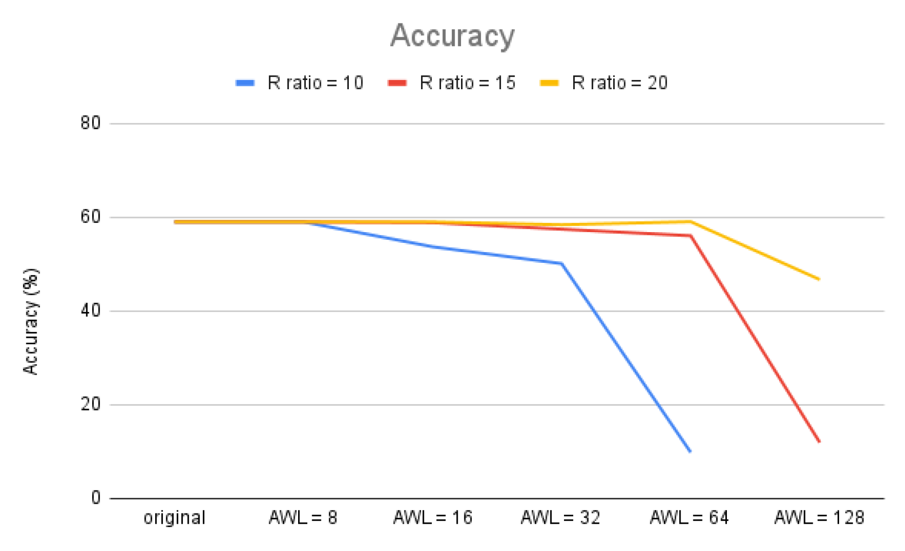
Figure 5.
Example of AWL effect on the calculation cycle and calculation error.
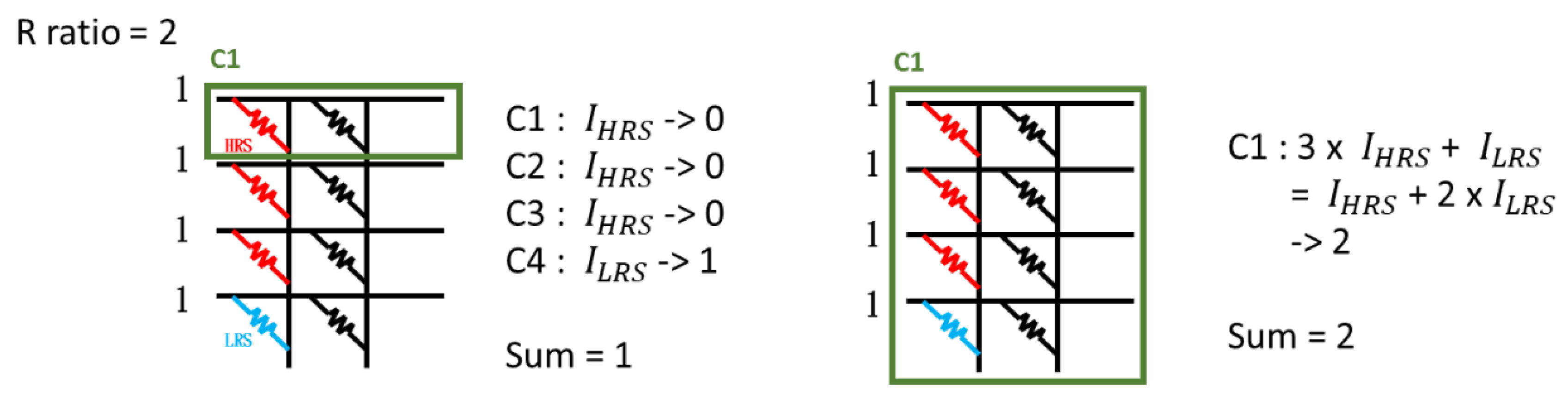
Figure 6.
Impact of the AWL on accuracy under R ratio 10.

Figure 7.
Accuracy of adjusting the AWL in a single layer with R ratio 10.
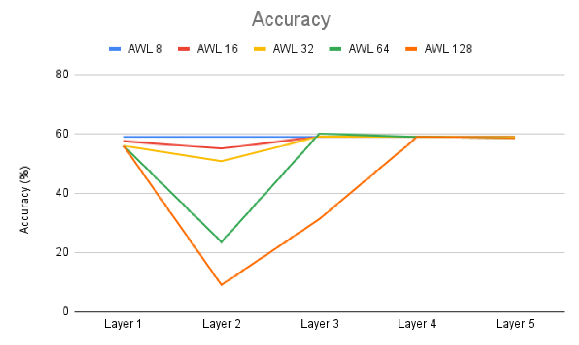
Figure 8.
The proportion of 0 in the weights in Cifar-10.
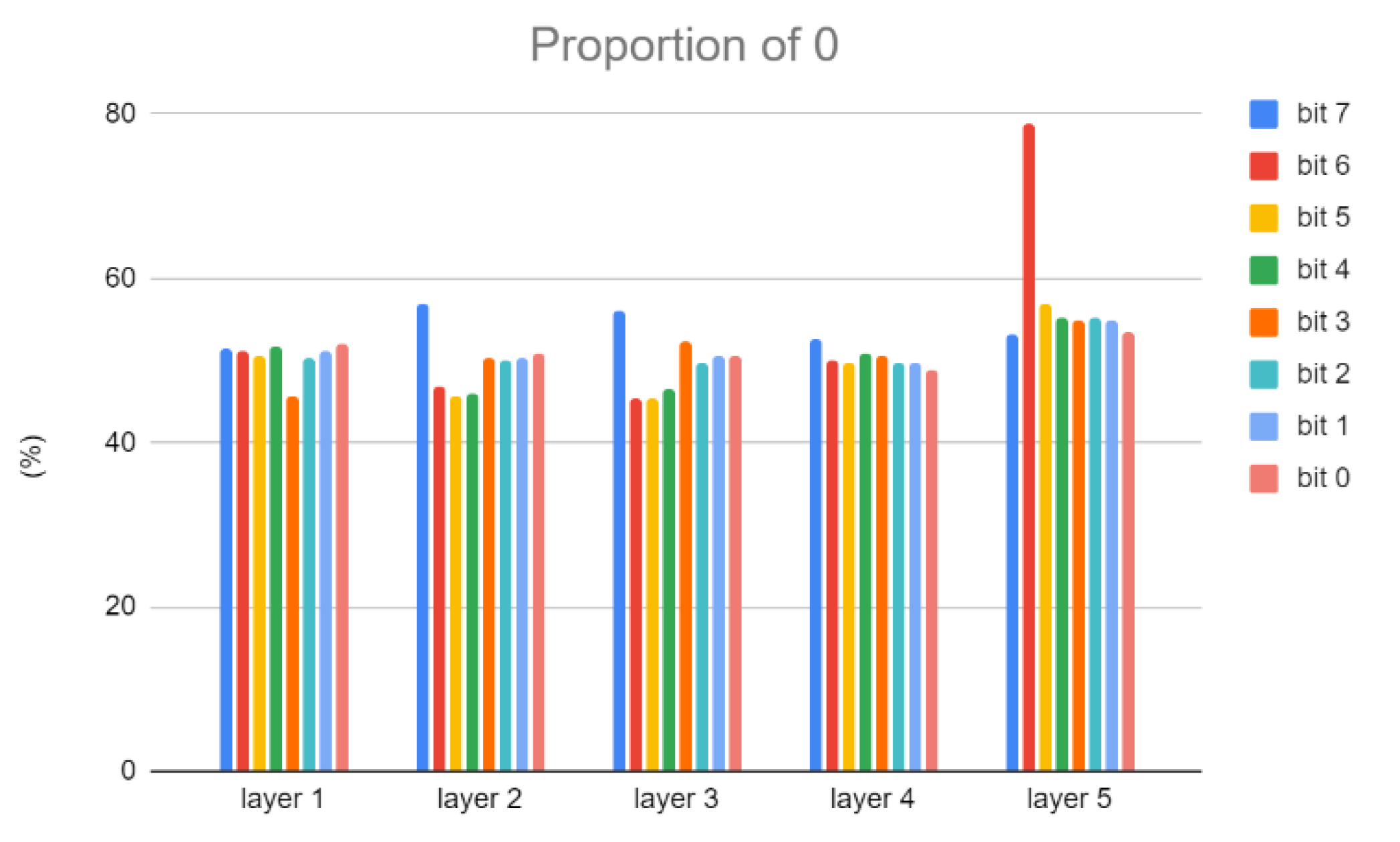
Figure 9.
The proportion of 0 in the weights in VGG-8.
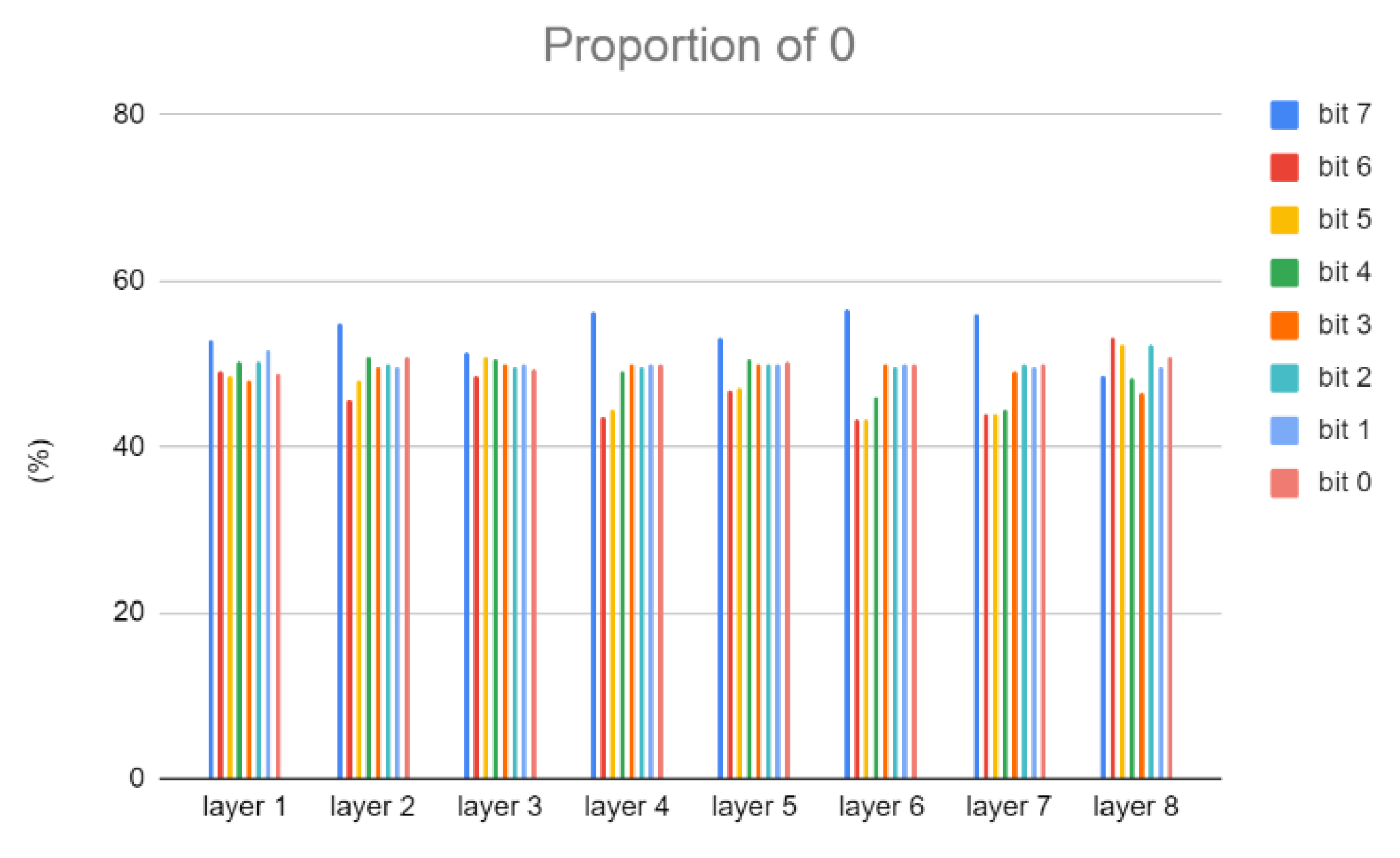
Figure 10.
Architecture of inference accuracy predictor.
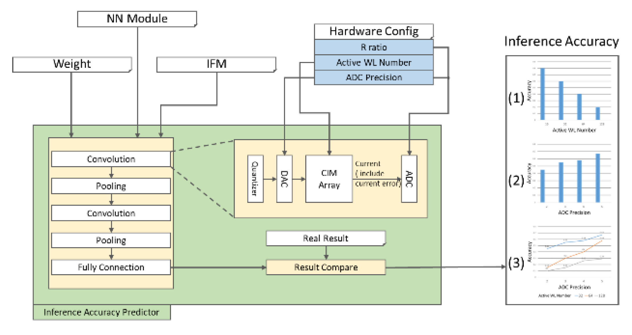
Figure 11.
Derivation of weight quantization.
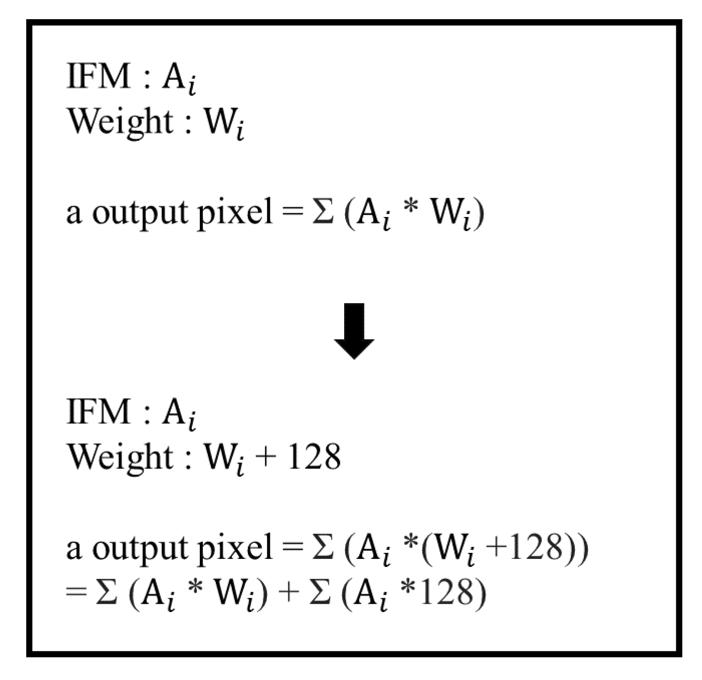
Figure 12.
Weight distribution of Cifar-10.
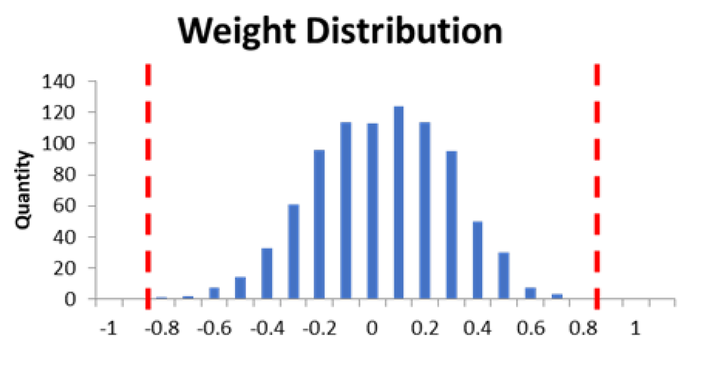
Figure 13.
Convolutional layer and fully connected layer operation process.
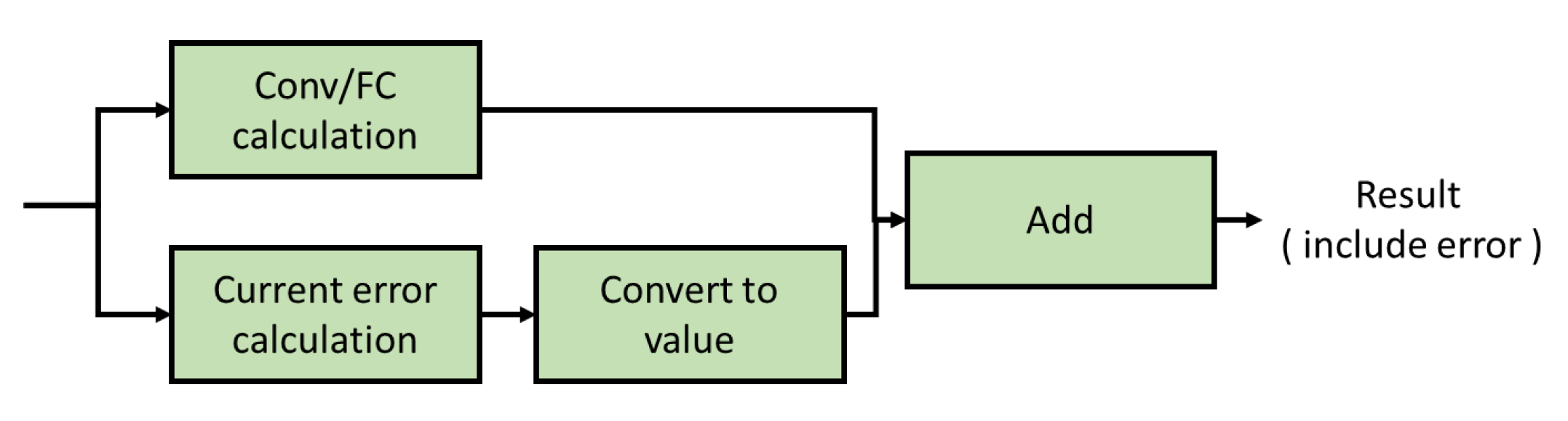
Figure 14.
Accuracy changing under different Min AWL (R ratio = 25).
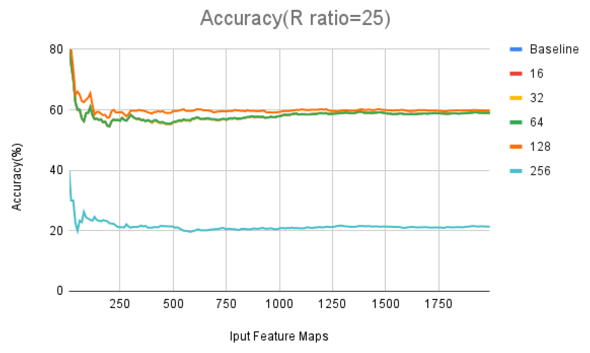
Figure 15.
Accuracy changing under different Min AWL (R ratio = 35).


Table 1.
Risk factors and their impact value on risk index.
| Risk Factor | Impact Value |
|---|---|
| R ratio <= 10 | +1 |
| Convolution Layer | +1 |
| Matrix Row (R) >= 256 | + |
| Ratio of 0 in MSB >= 55% | +1 |
| R ratio >= 20 | -1 |
| ( FC(Dense) Layer || Next Layer = FC Layer ) && R ratio > 10 |
-1 |
Table 2.
Risk index and corresponding AWL value.
| Risk Index | AWL |
|---|---|
| >3 (ratio <= 10) | 8 |
| >= 3 | 16 |
| 2 | 32 |
| 1 | 64 |
| <= 0 | 128 |
Table 3.
Experiment setup.
| Simulator | RRAM Accuracy Predictor |
| CNN | Cifar-10, VGG-8 |
| CIM array size | 512 * 512 |
| RRAM cell | 1 bit/pre cell |
| Resistance ON/OFF ratio | 10, 15, 20 |
Table 4.
Cifar-10 architecture.
| Input | Channel | Kernel | Depth | Matrix Row | Matrix Col. | |
|---|---|---|---|---|---|---|
| Layer 1 | 32 | 3 | 3 | 32 | 27 | 32 |
| Layer 2 | 15 | 32 | 5 | 64 | 800 | 64 |
| Layer 3 | 3 | 64 | 3 | 64 | 576 | 64 |
| Layer 4 | 1 | 64 | 1 | 64 | 64 | 64 |
| Layer 5 | 1 | 64 | 1 | 10 | 64 | 10 |
Table 5.
Cifar-10 layer-wise risk factor.
| Layer Type | Matrix Row | Ratio of 0 in MSB | |
|---|---|---|---|
| Layer 1 | Conv | 27 | 51.39 % |
| Layer 2 | Conv | 800 | 57 % |
| Layer 3 | Conv | 576 | 56.18 % |
| Layer 4 | Dense | 64 | 52.59 % |
| Layer 5 | Dense | 64 | 53.28 % |
Table 6.
Cifar-10 layer-wise risk index and AWL.
| Risk Index | Active WL Number | |||||
|---|---|---|---|---|---|---|
| R Ratio | 10 | 15 | 20 | 10 | 15 | 20 |
| Layer 1 | 2 | 1 | 0 | 32 | 32 | 32 |
| Layer 2 | 5 | 4 | 3 | 8 | 16 | 16 |
| Layer 3 | 5 | 3 | 2 | 8 | 16 | 32 |
| Layer 4 | 1 | -1 | -2 | 64 | 64 | 64 |
| Layer 5 | 1 | -1 | -2 | 64 | 64 | 64 |
Table 7.
VGG-8 architecture.
| Input | Channel | Kernel | Depth | Matrix Row | Matrix Col. | |
|---|---|---|---|---|---|---|
| Layer 1 | 32 | 3 | 3 | 32 | 27 | 32 |
| Layer 2 | 32 | 32 | 3 | 32 | 288 | 32 |
| Layer 3 | 16 | 32 | 3 | 64 | 288 | 64 |
| Layer 4 | 16 | 64 | 3 | 64 | 576 | 64 |
| Layer 5 | 8 | 64 | 3 | 128 | 576 | 128 |
| Layer 6 | 8 | 128 | 3 | 128 | 1152 | 128 |
| Layer 7 | 1 | 2048 | 1 | 128 | 2048 | 128 |
| Layer 8 | 1 | 128 | 1 | 10 | 128 | 10 |
Table 8.
VGG-8 layer-wise risk factor.
| Layer Type | Matrix Row | Ratio of 0 in MSB | |
|---|---|---|---|
| Layer 1 | Conv | 27 | 52.78 % |
| Layer 2 | Conv | 288 | 54.83 % |
| Layer 3 | Conv | 288 | 51.54 % |
| Layer 4 | Conv | 576 | 56.31 % |
| Layer 5 | Conv | 576 | 53.25 % |
| Layer 6 | Conv | 1152 | 56.76 % |
| Layer 7 | Dense | 2048 | 56.02 % |
| Layer 8 | Dense | 128 | 48.67 % |
Table 9.
VGG-8 layer-wise risk index and AWL.
| Risk Index | Active WL Number | |||||
|---|---|---|---|---|---|---|
| R Ratio | 10 | 15 | 20 | 10 | 15 | 20 |
| Layer 1 | 2 | 1 | 0 | 32 | 32 | 32 |
| Layer 2 | 3 | 2 | 1 | 16 | 32 | 64 |
| Layer 3 | 3 | 2 | 1 | 16 | 32 | 64 |
| Layer 4 | 5 | 4 | 3 | 8 | 16 | 16 |
| Layer 5 | 4 | 3 | 2 | 8 | 16 | 32 |
| Layer 6 | 6 | 4 | 3 | 8 | 16 | 16 |
| Layer 7 | 6 | 4 | 3 | 8 | 16 | 16 |
| Layer 8 | 1 | -1 | -2 | 64 | 128 | 128 |
Table 10.
Accuracy of Cifar-10 using layer-wise AWL.
| Active WL Number | |||
|---|---|---|---|
| R Ratio | 10 | 15 | 20 |
| Layer 1 | 32 | 32 | 32 |
| Layer 2 | 8 | 16 | 16 |
| Layer 3 | 8 | 16 | 32 |
| Layer 4 | 64 | 64 | 64 |
| Layer 5 | 64 | 64 | 64 |
| ACC | 55.65 % | 57.2 % | 58.35 % |
| Loss | -3.35 % | -1.8 % | -0.65 % |
Table 11.
Layer-wise computation cycle of Cifar-10.
| Baseline | R Ratio = 10 | R Ratio = 15 | R Ratio = 20 | |
|---|---|---|---|---|
| Layer 1 | 4 | 1 | 1 | 1 |
| Layer 2 | 100 | 100 | 50 | 50 |
| Layer 3 | 72 | 72 | 36 | 18 |
| Layer 4 | 8 | 1 | 1 | 1 |
| Layer 5 | 8 | 1 | 1 | 1 |
| Total | 192 | 175 | 89 | 71 |
| Benefit | X | -9 % | -54 % | -63 % |
Table 12.
Accuracy of VGG-8 using layer-wise AWL.
| Active WL Number | |||
|---|---|---|---|
| R Ratio | 10 | 15 | 20 |
| Layer 1 | 32 | 32 | 32 |
| Layer 2 | 16 | 32 | 64 |
| Layer 3 | 16 | 32 | 64 |
| Layer 4 | 8 | 16 | 16 |
| Layer 5 | 8 | 16 | 32 |
| Layer 6 | 8 | 16 | 16 |
| Layer 7 | 8 | 16 | 16 |
| Layer 8 | 64 | 128 | 128 |
| ACC | 62 % | 63.9 % | 64.79 % |
| Loss | -2.9 % | -1 % | -0.11 % |
Table 13.
Layer-wise computation cycle of VGG-8.
| Baseline | R Ratio = 10 | R Ratio = 15 | R Ratio = 20 | |
|---|---|---|---|---|
| Layer 1 | 4 | 1 | 1 | 1 |
| Layer 2 | 36 | 18 | 9 | 5 |
| Layer 3 | 36 | 18 | 9 | 5 |
| Layer 4 | 72 | 72 | 36 | 36 |
| Layer 5 | 144 | 144 | 72 | 36 |
| Layer 6 | 288 | 288 | 144 | 144 |
| Layer 7 | 512 | 512 | 256 | 256 |
| Layer 8 | 16 | 2 | 1 | 1 |
| Total | 1108 | 1055 | 528 | 484 |
| Benefit | X | -5 % | -52 % | -56 % |
Table 14.
Cifar-10 layer-wise risk index (large R ratio).
| Risk Index | ||
|---|---|---|
| R Ratio | 25 | 35 |
| Layer 1 | 0 | 0 |
| Layer 2 | 3 | 3 |
| Layer 3 | 2 | 2 |
| Layer 4 | -2 | -2 |
| Layer 5 | -2 | -2 |
Table 15.
Risk index and different min. AWL mapping table (large R ratio).
| AWL | |||||
|---|---|---|---|---|---|
| Risk Index | Min. AWL = 16 | Min. AWL = 32 | Min. AWL = 64 | Min. AWL = 128 | Min. AWL = 256 |
| >= 3 | 16 | 32 | 64 | 128 | 256 |
| 2 | 32 | 64 | 128 | 256 | 512 |
| 1 | 64 | 128 | 256 | 512 | 512 |
| <= 0 | 128 | 256 | 512 | 512 | 512 |
Table 16.
Accuracy and cycle benefit of Cifar-10 under different Min AWL (R ratio = 25).
| Active WL Number | |||||
|---|---|---|---|---|---|
| Min AWL | 16 | 32 | 64 | 128 | 256 |
| Layer 1 | 32 | 32 | 32 | 32 | 32 |
| Layer 2 | 16 | 32 | 64 | 128 | 256 |
| Layer 3 | 32 | 64 | 128 | 256 | 512 |
| Layer 4 | 64 | 64 | 64 | 64 | 64 |
| Layer 5 | 64 | 64 | 64 | 64 | 64 |
| ACC (%) | 59 | 59 | 58.9 | 59.65 | 21.14 |
| Loss (%) | -0 | -0 | -0.1 | +0.65 | - 37.86 |
| Cycle benefit (%) | -71 | -81 | -89 | -93 | -95 |
Table 17.
Accuracy and cycle benefit of Cifar-10 under different Min AWL (R ratio = 35).
| Active WL Number | |||||
|---|---|---|---|---|---|
| Min AWL | 16 | 32 | 64 | 128 | 256 |
| Layer 1 | 32 | 32 | 32 | 32 | 32 |
| Layer 2 | 16 | 32 | 64 | 128 | 256 |
| Layer 3 | 32 | 64 | 128 | 256 | 512 |
| Layer 4 | 64 | 64 | 64 | 64 | 64 |
| Layer 5 | 64 | 64 | 64 | 64 | 64 |
| ACC (%) | 59 | 59 | 59 | 59.15 | 51.83 |
| Loss (%) | -0 | -0 | -0 | +0.15 | -7.17 |
| Cycle benefit (%) | -71 | -81 | -89 | -93 | -95 |
Table 18.
Accuracy of Cifar-10 using layer-wise AWL (Min AWL = 32).
| Active WL Number | |||
|---|---|---|---|
| R Ratio | 10 | 15 | 20 |
| Layer 1 | 32 | 32 | 32 |
| Layer 2 | 32 | 32 | 32 |
| Layer 3 | 32 | 32 | 64 |
| Layer 4 | 64 | 64 | 64 |
| Layer 5 | 64 | 64 | 64 |
| ACC | 49.9 % | 57.35 % | 58.35 % |
| Loss | -9.1 % | -1.65 % | -0.65 % |
Table 19.
Accuracy of Cifar-10 using layer-wise AWL (Min AWL = 64).
| Active WL Number | |||
|---|---|---|---|
| R Ratio | 10 | 15 | 20 |
| Layer 1 | 32 | 32 | 32 |
| Layer 2 | 64 | 64 | 64 |
| Layer 3 | 64 | 64 | 128 |
| Layer 4 | 64 | 64 | 64 |
| Layer 5 | 64 | 64 | 64 |
| ACC | 9.85 % | 56.05 % | 59.6 % |
| Loss | -49.15 % | -2.95 % | +0.6 % |
Disclaimer/Publisher’s Note: The statements, opinions and data contained in all publications are solely those of the individual author(s) and contributor(s) and not of MDPI and/or the editor(s). MDPI and/or the editor(s) disclaim responsibility for any injury to people or property resulting from any ideas, methods, instructions or products referred to in the content. |
© 2025 by the authors. Licensee MDPI, Basel, Switzerland. This article is an open access article distributed under the terms and conditions of the Creative Commons Attribution (CC BY) license (http://creativecommons.org/licenses/by/4.0/).
Copyright: This open access article is published under a Creative Commons CC BY 4.0 license, which permit the free download, distribution, and reuse, provided that the author and preprint are cited in any reuse.


