
Submitted:
27 August 2025
Posted:
28 August 2025
You are already at the latest version
Abstract
We present \emph{Temporal Dynamics} (TD) as a time-first reparameterization of General Relativity (GR). In TD, mass sources a local slow-time fraction $\Delta T(\mathbf{x})$; keeping the universal converter $\mathrm{UC}=1/c$ exact implies that the straight-path delay over a segment of length $D$ corresponds to a curve-length increment $\Delta L=\overline{\Delta T}\,D$. Fixing the single TD mass constant to $k=4G/c^{2}$ (m\,kg$^{-1}$) makes the TD$\leftrightarrow$GR bridge exact: $\Delta L_{\rm rad}=r_s$, $\Delta L_{\rm diam}=2r_s$, and the TD horizon rule $D_{\rm BH}=kM$. The TD potential $\phi=-(c^{2}/2)\Delta T$ yields the general motion law $\mathbf{a}=(c^{2}/2)\nabla\Delta T$, reproducing the Newtonian limit $a_r=-GM/r^{2}$. Taking $\Delta T(r)=r_s/r$ reconstructs the Schwarzschild line element, so the PPN parameters match GR ($\beta=\gamma=1$) along with classic tests (gravitational redshift, light bending, Shapiro delay, perihelion precession). A variational formulation identifies $\Delta T$ with the ADM lapse via $N^{2}=1-\Delta T$; varying the action yields the Einstein equations with no extra propagating degrees of freedom (GR-equivalent dynamics, including gravitational waves with speed $c$ and GR polarizations/flux). Cosmologically, a residual micro-push $\epsilon$ per clock unit defines $\kappa=\epsilon/c$ and recovers the Hubble law $v=\kappa D$; constant $\kappa$ maps to $\Lambda=3\kappa^{2}/c^{2}$, while a slow drift $\kappa(z)$ corresponds to $w(z)\neq -1$, reframing the $H_{0}$ tension as differing $\epsilon_{0}$ estimates. TD thus organizes tested GR physics with a single constant $k$ and provides a micro$\to$macro interpretation of dark energy via $\epsilon$, without modifying GR’s empirical content.
Keywords:
general relativity
; Schwarzschild metric
; gravitational time dilation
; ADM formalism
; post-Newtonian parameters
; Shapiro delay
; light deflection
; dark energy
; Hubble constant
; cosmology
1. Introduction: The Cosmic Clock and the TD↔GR Dictionary
Temporal Dynamics (TD) is a time–first description of gravity and expansion. Building on earlier TD work [1], its basic premise is that gravitational phenomena can be organized by a single bookkeeping of time flow: where the local flow of time along an otherwise straight path is fractionally slower, the corresponding null path acquires exactly the extra length that General Relativity (GR) encodes as curvature. In this sense TD and GR are two languages for the same physics.
We refer to the conversion between time and length as the Universal Constant (s m−1), which turns a geometric length D into the empty–space traversal time . TD quantifies a path–averaged slow–time fraction (dimensionless) along a straight segment; the accumulated delay is
Converting back with gives the curve–length increment
This is the TD→GR bridge: slow time along a straight path corresponds to extra geometric length along the actual path.
Fixing a single mass constant
the bridge collapses to compact identities in the static, spherical sector:
where is the Schwarzschild radius. Thus a single constant k ties the TD time–delay bookkeeping to the familiar GR lengths.
The equivalence to GR may be stated more geometrically. In the static sector we identify the GR lapse with the TD time–offset via
so that . With the radial profile , this immediately reproduces the Schwarzschild line element and, therefore, all classic tests in the solar system (light deflection, Shapiro delay, perihelion precession, gravitational redshift). Linearizing the theory around flat spacetime yields two tensor polarizations propagating at speed c with the standard quadrupole energy flux; the gravitational–wave sector thus coincides with GR.
For cosmology, TD introduces a microscopic residual rate (an extra “push” per light–second unit) whose macroscopic imprint is
The late–time recession law is , so today and a constant is exactly a cosmological constant,
If desired, a gentle drift maps one–to–one to in the standard dark–energy language; distances, growth, and BAO/SNe/CMB inferences then proceed with the usual Friedmann machinery.
Scope and posture.
TD is presented here as a reparameterization of GR, not a modification: we write the Einstein–Hilbert action in TD variables and recover Einstein’s equations by variation. No new propagating degrees of freedom are introduced, and all tested predictions of GR are preserved. Conceptual pictures (e.g. viewing expansion via a global “cosmic clock”) are kept as interpretational aids; quantitative statements are anchored to the dictionary above.
Contributions.
(i) We establish the TD→GR bridge and, with , obtain the compact identities , , and . (ii) We construct the metric from and verify the PPN parameters (classic tests matched). (iii) We show that the linear gravitational–wave sector (polarizations, speed c, quadrupole flux) is identical to GR. (iv) We map the TD micro–parameter to the macroscopic cosmology via and , provide observable formulas (distances and growth), and outline a data strategy consistent with BAO/SNe/CMB analyses.
Organization.
Section 2 fixes notation and units. Section 3 develops the TD→GR bridge and a solar example. Section 4 gives the variational principle and the lapse identification. Section 5 builds the metric from ; Section 6 presents the PPN validation. Section 7 treats gravitational waves. Section 9 covers cosmology and observables. Conceptual notes and technical expansions appear in the Appendices.
2. The Mass Constant k: Definition, Units, and Equivalences
2.1. Purpose
To maintain continuity with prior TD papers [1] we retain the symbol k while fixing its definition and units so all TD results (gravitational acceleration, black–hole diameter, TD→GR bridge) are consistent and exactly aligned with GR.
2.2. Definition (Operational and Fundamental)
Operational (used throughout TD).
Fundamental equivalence (fixes the value by GR correspondence).
2.3. Units and Numerical Value
2.4. Unit Audit and Immediate Consequences
2.5. Canonical Identities (Single–Constant Form)
Scope: the following hold in the static, spherically symmetric exterior (vacuum) solution. Let .
- (1)
-
Schwarzschild match (any spherical mass).(See Sec. 5 for the line element derived from .)
- (2)
- Black–hole diameter (TD horizon rule). Horizon when :
- (3)
- Radial form (take ).
- (4)
- Potential and surface gravity (Newtonian limit). Define , then(Consistency with PPN is shown in Sec. 6.)
- (5)
- Total time delay across a diameter (mass–only invariant).
2.6. Backward–Compatibility
Symbol. We continue to write k to match earlier publications.
Units. Any occurrence of in older text should be corrected to . Prior formulas remain numerically consistent because was used as dimensionless and in meters.
Numerics. The prior value differs by ∼0.005%; fixing removes rounding and makes TD↔GR identities exact at the Schwarzschild scale.
2.7. Interpretation (What k Means)
- Mass → curve–length converter. k (m kg−1) tells how much effective path length space must add per unit mass to keep the universal clock exact: and .
- Built–in GR alignment. Since , one gets , and the horizon rule .
- Time–slowing as horizon fraction. With , —the local slow–time is literally the “how close to horizon” fraction.
- Newtonian limit. gives and automatically (see Sec. 6).
- Mass–energy view. Using , —a length per energy, echoing GR’s coupling scale.
- Null–path signature. The factor “4” echoes familiar lightlike coefficients in GR (e.g. deflection ), signaling that k encodes how light (or expansion at c) couples to mass in TD.
One–line meaning.
is TD’s mass–to–curve (mass–to–time–offset) proportionality that makes the TD time–delay and GR’s geometric curvature two faces of the same calculation, exactly.
Drop–in summary.
We retain the mass constant k for continuity and fix its value by the Schwarzschild correspondence: (m kg−1). Then is dimensionless and , , , , , , and the invariant diameter delay .
Fixing k from the Newtonian limit (one line)
Linearizing the Schwarzschild lapse gives so the potential is . TD defines with , hence .
Fixing k from the diameter delay
TD gives the mass–only invariant . Shapiro–type analyses isolate the same mass factor in the one–body limit; therefore .
3. TD→GR Bridge: Core Identity and Solar Example
This section establishes the algebraic bridge between TD’s path–averaged slow–time fraction and the geometric excess length that GR encodes as curvature. The result is a pair of identities that will be used repeatedly: a time-delay identity and a length identity. With (Sec. 2), these immediately reproduce the Schwarzschild scale.
3.1. Core Identities
Consider a straight segment of geometric length D through (or past) a mass M.
Empty-space traversal time.
Accumulated slow-time (TD).
If the path–averaged slow–time fraction is (dimensionless), the total delay is
Convert back to length (GR).
Multiplying by c gives the curve–length increment across the diameter:
For “radius–style” quantities:
Insert the operational TD law.
3.2. Worked Example: The Sun
Constants (SI): (exact), . Solar values: , .
TD time–offset (diameter).
Curve–length increments.
Schwarzschild check.
The Sun’s Schwarzschild radius is
matching within rounding, as predicted by Eq. (15).
3.3. Remark on Unit Handling (“No Double Conversion”)
3.4. Looking Ahead
4. Variational Principle and Field Equations for Temporal Dynamics (TD)
4.1. Aim and Philosophy
We present a variational formulation in which the TD “time–offset field” is not a new dynamical degree of freedom but a repackaging of the lapse function in the ADM form of General Relativity (GR). Varying the action yields the usual Einstein equations. In this sense, TD is a covariant reparameterization of GR: carries the causal interpretation (time slowdown), while the metric carries the geometry. This section makes that equivalence precise.
4.2. Minimal Setup and Units
Constants: c (speed of light), G (Newton’s constant), (units m kg−1). TD time–offset: (dimensionless).
ADM decomposition (shift-free for clarity).
TD identification (core dictionary).
4.3. Action
We take the standard Einstein–Hilbert action with matter, written in ADM variables, and express the lapse through :
with the identifications and (for clarity here) . Here is the Ricci scalar of , is the extrinsic curvature,
and denotes matter fields. A Gibbons–Hawking–York boundary term is understood to make the metric variation well-posed; it does not affect the bulk field equations and is omitted here for brevity.
4.4. Variations and Field Equations (Equivalence to GR)
Variation with respect to (Hamiltonian constraint)
Because ,
By the chain rule,
But is precisely the ADM Hamiltonian constraint:
where is the energy density measured by the unit normal to the spatial slice. Hence the “ equation” is not extra dynamics; it is exactly the GR Hamiltonian constraint.
Variation with respect to (evolution equations)
Variation with respect to the shift (momentum constraint)
If the shift is included, varying with respect to gives the ADM momentum constraints (equivalent to the mixed Einstein equations). In the present shift-free presentation they are trivially satisfied.
Takeaway.
The full GR field–equation content (Hamiltonian and momentum constraints, plus evolution equations) is recovered by varying the TD–augmented action. The “TD field equation” is exactly the Hamiltonian constraint; TD introduces no extra gravitating degree of freedom.
4.5. Static, Spherically Symmetric Sector (Schwarzschild)
In vacuum and static symmetry, and we may set for the Schwarzschild case. The Hamiltonian constraint reduces to on each slice, and the evolution equations fix the 3-metric together with the lapse N to the Schwarzschild solution. In TD language this is
recovering Sec. 5. All classic tests (light deflection, Shapiro delay, perihelion advance, gravitational redshift) follow because the line element is Schwarzschild.
4.6. Cosmology (Consistency with and H)
In homogeneous, isotropic slicing (FLRW) with zero shift, the ADM action reduces to the standard cosmological action. Choosing implies for the background clock (as usual in comoving time). A cosmological constant gives . The TD dark–energy dictionary identifies
so the GR sector and the TD micro–rate are in one–to–one correspondence. Linear perturbations proceed in the usual way; TD does not add a propagating scalar beyond GR.
4.7. Covariant “Link” Formulation
To make the identification manifestly covariant, introduce a scalar “clock” field whose level sets define the time foliation. Define the (future–pointing) unit normal to slices by
The lapse is . Impose the TD link via a Lagrange multiplier:
Variations give: and on–shell; the Einstein–Hilbert dynamics are unchanged. This simply ties to the foliation without introducing new dynamics.
4.8. Interpretation and Novelty
- plays the role of the lapse via (21). Varying enforces the Hamiltonian constraint; there is no extra dynamical scalar.
- The action principle is GR’s action written in TD variables. Hence the field equations are exactly Einstein’s equations.
- The novelty is interpretational and organizational: the single constant and the TD time–offset bookkeeping yield compact, mass–only identities (e.g., ) and a micro–to–macro path for cosmic acceleration () without modifying GR’s tested predictions.
4.9. What Would Change TD into a New Theory (and Why We Do Not Do That Here)
If one added a genuine kinetic term for (e.g., gradients of in the Lagrangian), would become dynamical and generally produce deviations from GR (extra propagating modes, fifth forces, or modified wave speeds). We do not introduce such terms; TD is presented here as a reparameterization of GR with a causal interpretation, not as a modification.
Boxed field–equation summary (TD form)
Action (bulk):
TD dictionary: (so ).
Variations: Hamiltonian constraint (GR); evolution equations (GR); momentum constraints (if shift included).
Static spherical vacuum: , , .
Cosmology: , , .
5. Metric Construction from
This section builds the static, spherically symmetric line element from the TD radial profile
and the dictionary (so ). Building on Sec. 4, we now recover the Schwarzschild metric.
5.1. Ansatz and TD Dictionary
For a static, spherically symmetric vacuum exterior we write
with . The TD dictionary fixes the lapse via
Thus is fixed by TD; it remains to determine .
5.2. Fixing the Radial Factor from Vacuum Einstein Equations (Sketch)
5.3. Result: Schwarzschild Line Element
5.4. Immediate Checks
(i) Gravitational redshift / proper time.
From (31), clocks at fixed r satisfy , which equals the TD rule once .
(ii) Radial null rays and the horizon.
Setting gives so is a null surface (the horizon). This matches the TD “horizon rule” at .
(iii) Weak–field expansion and PPN match.
For ,
and
Reading off the Parametrized Post-Newtonian coefficients gives , which we collect and test in Sec. 6.
5.5. Summary of the Construction
TD fixes the lapse via the slow–time profile ; imposing the vacuum Einstein equations then determines the radial factor and returns the unique exterior solution (31). Thus the TD time–offset bookkeeping and GR geometry are exactly equivalent in the static, spherical sector.
6. PPN Validation of Temporal Dynamics (TD)
6.1. Goal and Strategy
We show that TD makes the same first–post-Newtonian (PPN) predictions as General Relativity (GR). Strategy: (i) build the line element from ; (ii) expand to 1PN in isotropic coordinates and read off ; (iii) list classic tests and verify agreement.
Conventions.
(Schwarzschild radius), (positive magnitude), , and the local TD clock relation .
TD motion law (Newtonian limit).
With one has ; for this gives .
6.2. Line Element from (Schwarzschild Sector)
From with we have
Spherical vacuum fixes , with angular part . Thus
Because this is Schwarzschild, TD inherits all GR test results; the PPN check below makes this explicit.
6.3. PPN Extraction
The PPN template (isotropic spatial metric) to 1PN is
Write Schwarzschild in isotropic radius using
which gives the exact form
Define and note at this order. Expanding for :
Comparing with the template yields
and (in this static, spherically symmetric vacuum) vanishing preferred–frame parameters (), i.e. the GR point in PPN space.
6.4. Classic Tests (TD = GR)
Gravitational redshift / time dilation.
From TD: . Weak field: . Frequency shift between and :
Deflection of light by mass M.
PPN: . With : ( for a grazing solar ray).
Shapiro time delay (radar echo).
Near superior conjunction, one–way extra delay for impact parameter b and endpoints :
With : coefficient (one–way); round–trip doubles to .
Perihelion precession (bound orbits).
PPN per–orbit advance:
With : (e.g. for Mercury after Newtonian perturbations).
6.5. Scope and Coordinates
The extraction uses isotropic coordinates because the PPN template is defined there; the TD metric in standard Schwarzschild coordinates (33) is coordinate–equivalent at this order. For rotating sources (Kerr), additional frame–dragging terms enter the full PPN counting; TD as formulated here (static mapping with ) covers the non–rotating sector. Extending the dictionary to rotation is left for future work.
Boxed results (quick reference)
Metric (TD): .
PPN: , , (static, spherical vacuum).
Light deflection: .
Shapiro delay (one–way): .
Perihelion precession: .
Redshift: (weak field). (See Table 1).
7. Gravitational Waves: TD = GR in the Radiative Sector
7.1. Claim and Scope
Temporal Dynamics (TD) introduces no new propagating degree of freedom: is a repackaging of the lapse (; Sec. 4). Therefore the radiative sector coincides with GR: two transverse–traceless tensor polarizations, waves propagate at c, and the far–zone flux is the standard quadrupole formula. This section shows the equivalence by linearizing around flat spacetime.
7.2. Linearization and Gauge
Linearize the metric about Minkowski:
In ADM language with vanishing background curvature, and at zeroth order. A first–order perturbation of the TD field appears only through the lapse perturbation ; since has no kinetic term (Sec. 4), its variation enforces a constraint rather than a wave equation. After imposing the linearized constraints (Hamiltonian and momentum), the two radiative tensor modes in remain, just as in GR.
7.3. Propagation Speed and Polarizations
In vacuum (), Eq. (41) reduces to
whose plane–wave solutions travel at speed c. In the transverse–traceless (TT) gauge, only the spatial components survive and are traceless and transverse:
For a wave propagating along ,
revealing the two tensor polarizations , identical to GR.
7.4. Far–Zone Solution and Energy Flux
In the slow–motion, weak–field source regime, the far–zone TT strain at distance R is
where is the (trace–free) mass quadrupole moment of the source. The averaged GW stress–energy (Isaacson) is
which yields the standard quadrupole luminosity
and the energy flux at large R. Equations (45)–(47) are the GR results and follow here because TD introduces no extra wave modes and no modified couplings.
7.5. Observational Mapping
Because the wave equation, polarizations, speed, and flux are all the GR ones, TD makes the same quantitative predictions for compact–binary inspirals: phase evolution (chirp), amplitude–distance relation (standard sirens), and polarization response in detector networks. In particular, the propagation speed equals c and no scalar/vector polarizations are present, aligning TD with the current interferometer constraints.
Boxed Results (Quick Reference)
Wave equation (vacuum): (speed c).
Polarizations: two tensor modes in TT gauge.
Far–zone strain: .
Power: .
TD role: is non-propagating (lapse), so no extra GW modes; TD = GR for GWs.
8. Dark Energy from Temporal Dynamics (TD)
8.1. Postulates
(1) Cosmic clock (normal expansion).
Space expands at the universal clock rate set by light. Define the cosmic unit length
(one light–second of length). Earlier sections used (s m−1); here we work in lengths, so there is no conflict.
(2) Residual field (dark energy).
Today’s space carries a faint residual “push” per unit per second, denoted . Units: has dimensions of m s−2 per cosmic unit (i.e., extra velocity gained each second per light–second of separation).
8.2. Geometry of Separation
For two masses at physical distance D, the number of cosmic units (light–second lengths) between them is
8.3. Residual Expansion Adds Linearly Over Units
Each unit contributes (m s−2) of extra velocity per second. Over one second, summing across N units gives the recession speed due to dark energy:
8.4. Macroscopic Residual Rate and Hubble Identification
Define the macroscopic residual rate
so that the TD recession law is
Comparing with Hubble’s law gives
Thus, in TD, is not free; it is derived from the micro–rate .
8.5. Deriving and from Observations
Given a single galaxy (peculiar motion removed) with measured recession speed and proper distance :
Step 1 — solve for .
Illustrative example.
Step 2 — from to .
8.6. Time Evolution / Acceleration (Optional)
If (hence ) varies with cosmic time,
With constant (de Sitter) and ,
8.7. Units and Symbols (Quick Check)
Summary box (key results)
Core law: . Macroscopic rate: . Hubble identification: .
Inference from data: . Constant : (de Sitter–like).
9. Cosmology from TD: Friedmann Equations, Mapping, and Observational Constraints
9.1. Setup (TD → Macro)
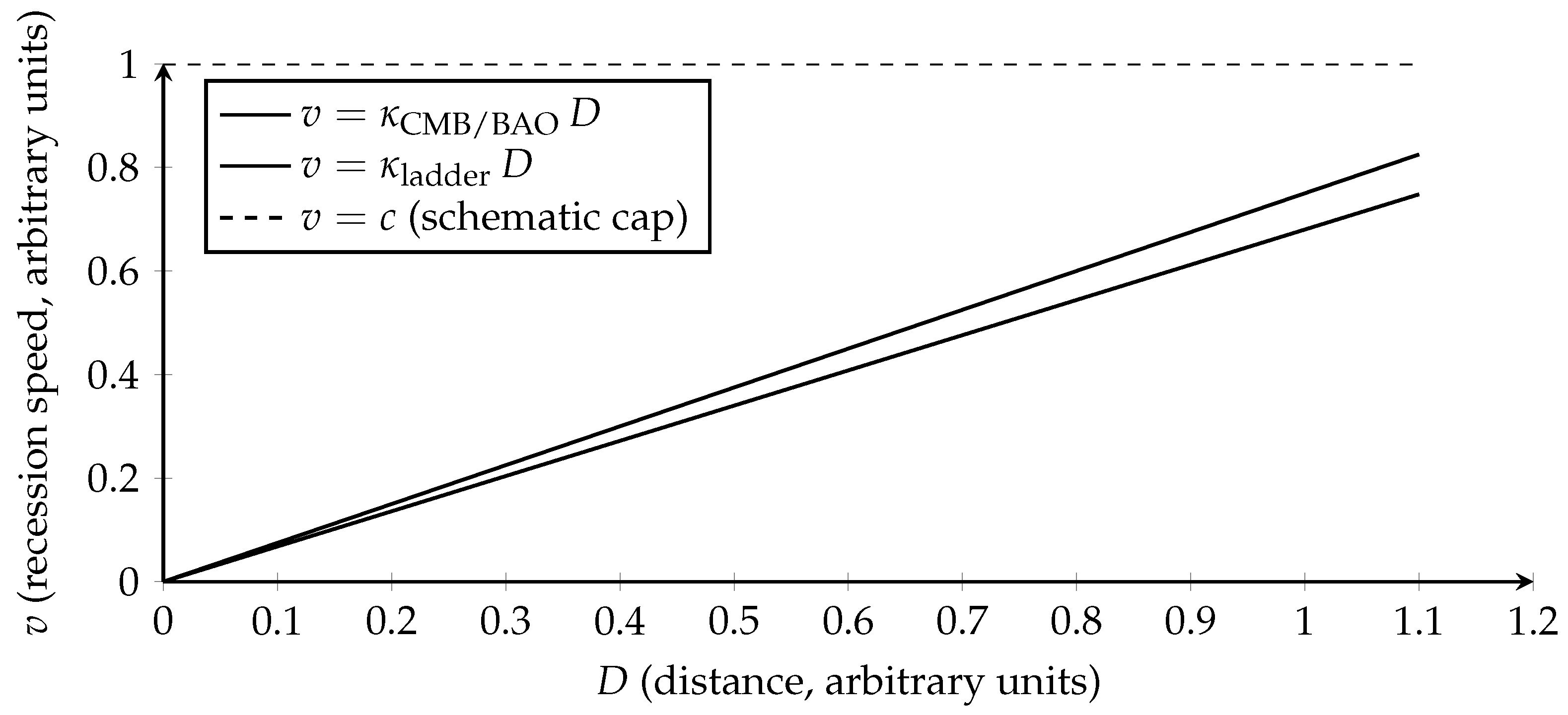
Micro parameter: (per–unit residual push, m s−2 per ). Macro rate: (s−1). TD recession law: . In homogeneous, isotropic FLRW, treat as the dark–energy driver. (See Figure A2).
9.2. Friedmann Equations in TD Variables
A constant corresponds exactly to a cosmological constant:
Then the Friedmann pair (curvature ) reads
In a flat matter+ case,
9.3. If Varies with Time
Define . The continuity equation gives an effective equation of state
In DE–domination () this reduces to .
9.4. Background in Terms of Redshift
With and flat geometry,
Two common calibrations: (i) TD–dominant late time (heuristic): . (ii) GR split (exact): with in flat space. In either case, is the micro residual rate today.
9.5. Distances and Observables
Given from Eq. (63),
Thus SNe (via ), BAO (via and ), and CMB (via the acoustic angle) are computed as usual once is specified.
9.6. Growth of Structure
TD does not modify gravity (Sec. 4); linear growth follows the GR equation in the chosen background:
Predictions for and lensing therefore match GR given the same .
9.7. Numerical Mapping ()
By Definition :
(Use m s−1 and m. Values shown are illustrative.)
9.8. Observational Constraints and the Tension (TD View)
In TD, the tension is simply two estimates of the same micro rate : an early–time inference (CMB/BAO–anchored) versus a late–time distance–ladder inference. If is constant, TD reduces to CDM (). Allowing a mild late drift corresponds to via Eq. (62), offering a controlled way to adjust local while preserving early–time observables.
Boxed identities (cosmology)
; ; ; .
. . .
10. Observables, Parameterizations, and Data Strategy for TD Dark Energy
10.1. Distance–Redshift Relations (SNe and BAO)
Use from Sec. 9 (Friedmann with ):
Flat baseline: , with and . For curvature, add in and use the standard prescription for distances.
10.2. Linear Growth of Structure (RSD and Weak Lensing)
TD (as presented) is GR–equivalent for background and linear perturbations, so
where primes denote . A useful summary is with for CDM; mild shifts slightly.
10.3. Parameterizing (or )
Option A (direct TD).
Option B (CPL equation of state).
10.4. Curvature and the Sound Horizon (Degeneracies)
Allow if needed: For BAO, specify whether (sound horizon) is fixed by an early–universe prior (CMB–informed) or floated in late–time–only fits.
10.5. Minimal Fitting Workflow (Practical)
- Choose geometry: flat by default () unless testing curvature.
- Choose parameterization: constant () or one of the drifts above.
- Compute , then , , , .
- Growth: integrate or use for RSD/lensing likelihoods.
- Likelihoods: combine SNe (distance moduli), BAO (, ), and CMB anchors (acoustic angle or prior) as appropriate.
- Report posteriors for and derived .
- Model comparison: if you freed , quote AIC/BIC against constant .
Boxed formulas (quick reference)
;; ; ; .
; ; ; .
Growth: ; (near ).
Worked numerical example (from to and )
Constants.
, , .
Definitions.
in s−1: .
TD micro rate: . Mapping: , .
Calibration A (GR split; flat CDM).
Here .
Example A1 (Planck-like): .
Example A2 (ladder-like): .
Calibration B (TD late–time heuristic; DE-dominated).
Here (pure de Sitter at late times).
Example B1: .
Example B2: .
Comment.
Calibration A (GR split) uses the measured and reproduces the standard values; Calibration B (TD heuristic) is appropriate only in a DE-dominated asymptotic view where . In all cases the TD micro value follows transparently as .
11. Conclusions
We presented Temporal Dynamics (TD) as a time-first reparameterization of General Relativity (GR). The single mass constant makes TD’s path-averaged slow-time quantitatively equivalent to GR curvature: and . From the variational principle (Sec. 4), varying enforces the Hamiltonian constraint, so TD introduces no new degrees of freedom. The metric built from (Sec. 5) is Schwarzschild; the PPN parameters (Sec. 6) are ; gravitational waves (Sec. 7) have the GR tensor polarizations, speed c, and quadrupole flux.
In cosmology (Sec. 9), a uniform micro residual rate maps to a macroscopic rate and to . Constant reproduces CDM; mild late-time drift is equivalent to in the standard language and can be constrained by BAO/SNe/CMB and growth.
Outlook.
Natural next steps include: (i) extending the TD dictionary to rotation (Kerr and Lense–Thirring), (ii) a full cosmological perturbation treatment with fits, and (iii) exploring whether TD’s bookkeeping yields new compact analytic identities (e.g., lensing integrals, timing delays) useful for data analysis. TD, as formulated here, is observationally GR-equivalent in the tested regimes; any phenomenology beyond GR would arise only if were promoted to a dynamical field (which we do not do here).
Author contributions
Conceptualization, formal analysis, writing, and verification: O. O. Francis.
Competing interests
The author declares no competing interests.
Data and code availability
No new datasets or custom code were generated. Numerical values use standard physical constants; all reproducible numbers are given in the text and appendices.
Acknowledgments
I thank OpenAI’s ChatGPT for interactive help with algebraic rearrangements, unit/notation checks, and LaTeX formatting during the preparation of this manuscript. All derivations, physical interpretations, and final text were produced and verified by the author; any errors are mine alone. No external funding was received for this work. I am grateful to the Overleaf community for tooling and to the anonymous referees for their time and comments.
Appendix L Conceptual Notes: The Cosmic Clock and TD Intuition
Appendix L.1. The Cosmic Clock and the Unit Length L★ = c
The starting picture is a universal clock: for every second of time, light marks out exactly one light–second of length. Two equivalent conversion constants are useful:
Earlier sections sometimes use (time per length) while here we use (length per second). They are reciprocals, so switching between “time-first” and “length-first” viewpoints is straightforward.
Intuition.
Think of the universe as a giant metronome: every tick of duration lays down of “clock length” in every direction. TD asks: what happens to this steady mapping between time and length when mass or a residual cosmic push is present?
Appendix L.2. Two Rulers: Straight Time vs. Curved Space
GR measures how paths bend: the geometry between two points becomes longer than the Euclidean straight line. TD measures how the straight path’s local time slows by a fraction ; to keep the global clock exact, space “adds” just enough extra length along the actual path.
Bridge identity.
If a straight segment has geometric length D and a path–averaged slow–time fraction ,
No double conversion: multiply by once to get a time delay, then multiply by c once to get a length increment.
Sun thought experiment.
For a diameter through (or a limb–skimming chord past) the Sun, using and gives , matching the Schwarzschild scale. GR’s curved surface length and TD’s straight–path slow–time are two readings of the same mass effect.
Appendix L.3. Mass as Concentrated Time; the Meaning of k = 4G/c2
TD uses one constant
so that
Interpretations:
- Length per mass. k tells how many meters of effective path length are “added” per kilogram to preserve the universal clock.
- Per energy. Using , is the same meter-per-joule scale that appears in GR’s coupling (compare ).
- Horizon fraction. With , .
- Diameter invariant. The mass-only time delay across a diameter is .
Appendix L.4. Where Gravity “Comes from” in TD Language
In weak fields, define a potential
With this gives and
TD says: matter drifts toward regions where local time runs slower (larger ), which is equivalent to sliding down . GR says: free fall follows geodesics in the curved metric. Both statements describe the same motion.
Appendix L.5. Dark Energy as a Residual Micro–Push
TD posits a tiny per–unit residual push (m s−2 per light–second). Over a separation D there are units, so in one second the extra recession is
Define the macroscopic rate (s−1). Then
Constant reproduces CDM (). A slowly drifting is equivalent to via
What observations “measure.”
A direct slope of v vs. D at low z gives ; then . Early–time probes (CMB+BAO) infer indirectly through the background expansion; late–time distance ladders infer it locally. In TD language the tension is two estimates of the same micro rate .
Appendix L.6. What TD Does Not Change
- Field equations. The variational principle with reproduces Einstein’s equations; is not a new propagating field.
- Solar–system tests. PPN parameters are ; light bending, Shapiro delay, perihelion advance, and redshift match GR.
- Gravitational waves. Two tensor polarizations, speed c, and quadrupole flux; same wave equation as GR.
- Early universe. TD does not modify pre–recombination physics at the background or linear level; the sound horizon and CMB acoustic physics are unchanged once (or ) is specified.
- Causality and c. The speed of light is constant; TD never requires c to vary.
Appendix L.7. What Would Make TD a New Theory (and Why We Avoid It)
Promoting to a dynamical field by adding gradient or kinetic terms in the action would introduce an extra scalar mode (“fifth force”), alter wave speeds, and generically deviate from GR. The formulation in this paper deliberately does not add such terms: TD is GR in time–first coordinates.
Appendix L.8. Frequently Asked Questions
Why ΔT(r) = rs/r?
Because TD fixes the lapse via and matches the Newtonian limit through . This pins , which then yields the Schwarzschild metric.
Does TD Change Coordinates?
No. TD gives a dictionary for the lapse; the resulting metric is Schwarzschild in standard coordinates. For PPN comparisons one passes to isotropic coordinates in the usual way.
Is the factor “4” in k = 4G/c2 special?
Yes: it encodes null–path effects (e.g., for light deflection) and ensures the diameter invariant .
Is the residual ϵ just H0c?
At , yes: . If drifts, maps one–to–one to .
What about rotation and frame dragging?
This paper treats the static spherical sector. Extending the TD dictionary to include off–diagonal pieces recovers Lense–Thirring and, in full, the Kerr metric (left for future work).
How should I think about gravitational waves in TD?
As tiny, transverse ripples in how the global clock synchronizes across space; mathematically they are the same tensor waves GR describes.
Appendix L.9. Minimal TD↔GR Dictionary (One Page)
- (m kg−1); ; ; .
- ; ; ; .
- ; .
- (m s−2 per ); (s−1); ; ; .
Appendix L.10. Common Pitfalls (and Quick Fixes)
- Double converting time and length. Use then .
- Mixing and . Work either in time–per–length () or length–per–time () consistently; they are reciprocals.
- Treating as clock time, not a fraction. is dimensionless (a “seconds per second” fraction). The actual delay is .
- Forgetting is per unit . The macroscopic law is , not .
Appendix L.11. Roadmap Back to the Mathematics
Appendix L.12. Normal Expansion (the Baseline Clock Field)
Definition.
The normal expansion is the global mapping between time and length set by light:
By itself, this clock field acts uniformly everywhere. Two co–moving masses that share the same frame do not acquire relative motion from the normal expansion, because there is no differential between them.
Operational statement.
Let D be the physical separation between two co–moving masses. The normal expansion contributes the same of coordinate time along either worldline; therefore it creates no separation. Relative motion arises only from (i) gravity (through gradients), (ii) peculiar velocities, or (iii) the residual “micro push” summed over units (Sec. 8).
Appendix L.13. TD Gravity Ratio and the General Motion Law
Local clock ratio (the right “gravity ratio”).
In TD (and GR), the local slow–time factor is
We call the gravity ratio. It is dimensionless, , and exactly reproduces gravitational redshift/time–dilation.
Lvoid a common pitfall (path fraction vs. local ratio).
If one forms the path fraction
this is a path-averaged ratio, not a local clock factor. Here
For small , while the correct local ratio is . Use for dynamics and clocks.
Flow speed and the “never crosses c” statement.
Define the local flow speed of the clock field
As , decreases but never exceeds c. This captures the intuition that gravity “slows the flow” locally.
General motion law (weak field / Newtonian limit).
The acceleration of a slow test particle follows from the TD potential
For a point mass with ,
i.e. the standard Newtonian acceleration. Thus TD’s dynamics are encoded in the gradient of , not in the difference .
Relation to the velocity-style heuristic.
The heuristic “c minus gravity ratio times c” is a good intuition for a local speed deficit:
But has units of speed; acceleration comes from spatial variation:
which reproduces Eq. (A76) exactly when you use the TD potential .
Boxed: TD motion and ratios (quick reference)
Local gravity ratio: . Clock flow speed: . TD potential: . General motion law: . Point mass: .
Worked example: Earth surface gravity (numbers).
Constants. , , , .
Schwarzschild scale.
Local slow–time at the surface.
Clock-flow “speed deficit” (intuition only).
Acceleration from the TD motion law. Using and ,
which equals the Newtonian result to the stated precision.
Lssumptions and domain (scope of formulas)
Unless stated otherwise, we assume: static, spherically symmetric, exterior region ; weak–field expansions use . Coordinates are Schwarzschild (standard) unless noted; isotropic coordinates are used only for PPN matching. Local slow–time is ; path-averaged quantities carry a bar, e.g. . Units. c exact (SI); (CODATA 2018 [2]).
Notation (quick reference)
(s m−1): time-per-length converter. (m per s): length per tick (one light-second). (m kg−1). . (local, dimensionless); (path average). . (m s−2 per ); (s−1).
Appendix L.14. Dark Energy as a Residual (“Twin”) Expansion: An Expanded Intuition
Dark energy has long been described operationally as a negative–pressure component that accelerates expansion. TD adds a causal picture: the universe carries a faint residual expansion imprint, a micro push per light–second (Sec. 8), left over from an earlier, faster epoch. Summing this imprint across many clock units reproduces the macroscopic Hubble law and, in GR variables, is exactly a cosmological constant (or a mild if the imprint drifts).
Normal expansion vs. relative motion.
- Cosmic clock field. The normal expansion is the global mapping (Sec. L). It acts uniformly and synchronously, so two co–moving masses sharing the same frame do not separate because of it.
- No differential, no drift. If gravity between and vanishes and both are co–moving, their relative motion from the clock alone is zero. TD and GR agree: relative motion requires a differential driver (gravity, peculiar velocity, or—in TD—the residual micro push).
Why dark energy is not the normal clock.
If the normal clock itself created relative motion, any two co–moving galaxies would drift apart purely from the background, contrary to how the FRW frame is defined. TD therefore separates:
The residual does create relative motion because its effect adds across the units between two points.
The “twin expansion” hypothesis (cartoon).
Think of two expansion signatures:
- Normal expansion: defines the spacetime ruler (the clock) and keeps c exact.
- Dark expansion: a faint twin with a slightly different temporal rate.
The mismatch leaves a residual “memory” per unit, . Across a separation D there are units, so in one second the extra recession is
Thus the farther the separation, the larger the accumulated residual and the larger the recession speed—exactly the observed linear law. In GR variables,
so a constant is indistinguishable from CDM at the background level (Sec. 9).
Light and temporal signatures.
- No second metric. TD remains single–metric GR (Sec. 4). The normal clock sets the null cone; locally measured light speed is c, everywhere.
- Operational view. Light is bound to the normal clock: it rides the same lapse that defines time flow. The residual expansion never introduces a new propagation channel; it only changes the background rate that distances accumulate against (hence , , etc.).
Putting the pieces together.
- Cause. A past, faster phase left a uniform micro residual per unit, .
- Effect. Summed over units, it yields .
- GR face. maps to (constant case) or to (drifting case).
Figure A2.
TD dark energy as a residual rate : recession is . Different data combinations infer slightly different slopes (the tension recast as or ).
Figure A2.
TD dark energy as a residual rate : recession is . Different data combinations infer slightly different slopes (the tension recast as or ).
Referee-facing clarifications.
- Not bimetric: There is no second metric or extra mode; is an auxiliary lapse variable, not a propagating field.
- Energy–momentum: The residual maps to an effective with , the standard GR vacuum form.
- Predictions: Constant ⇒CDM. Mild late drift in ⇒ standard – phenomenology. Discriminants are BAO/SNe distances, CMB acoustic angle, and growth (Sec. 10).
One–paragraph summary.
In TD, the universe’s acceleration is not a new force but an echo of its own past: a tiny, uniform residual micro push per light–second, , accumulated across many units into a macroscopic rate . This reproduces Hubble’s law and maps one–to–one to GR’s (or to if drifts), while preserving a single metric, local c, and all tested GR phenomenology.
Appendix L.15. What “One Unit of Space per Second” Really Means
The clock unit is a conversion, not a wind.
TD uses two reciprocal constants to translate between time and length:
Saying “one unit of space per second” means one light–second of length corresponds to one second of time by definition of c. It does not mean space streams past objects adding c meters every second.
Replication vs. addition (the cartoon vs. the math).
The “each unit replicates every second” image is a cartoon for counting. The mathematics is continuous:
- Normal clock (shared): contributes equally to all co–moving worldlines. Two co–moving masses separated by D remain at fixed comoving separation from the clock alone: no differential ⇒ no relative drift.
-
Residual push (dark energy): a tiny per–unit imprint (m s−2 per ) does sum across the units, giving in one secondThis is Hubble’s law in TD variables. If is (approximately) constant, the separation solves (de Sitter).
Mapping to FRW (no new physics).
In an FLRW background with scale factor , TD’s is just the vacuum component in the Friedmann equations:
Constant reproduces CDM (); a slow drift is a standard model via .
No “space wind,” no second metric.
Local physics uses the single GR metric; light speed is c everywhere. The clock unit is a bookkeeping device (a ruler synchronized to c), not a fluid that flows through matter.
A 30-second thought experiment.
Place two free test masses that are co–moving (no peculiar velocity, no mutual gravity) at separation D.
- Normal clock only: both accumulate the same coordinate time per light-second; separation remains D.
- Add residual ϵ: across units, one second later their relative velocity gained is . This is the observed late-time acceleration.
Units sanity check.
Dimensional chain: gives .
Edge cases and scope.
All statements here refer to the exterior region and to background expansion at sub-horizon scales where the FLRW picture applies. Normal expansion produces no local relative motion between co–moving masses; relative drift arises from (gravity) or from (the residual).
Glossary (mini–card)
- c
- Speed of light; sets the clock length .
- Universal converter (s m−1), time↔length.
- G
- Newton’s constant.
- k
- TD mass constant (m kg−1); mass→curve converter.
- Schwarzschild radius .
- Local slow-time fraction (dimensionless).
- Path-averaged slow-time fraction along a segment.
- Local gravity ratio .
- TD potential .
- Motion law (Newtonian limit) .
- Curve–length increment for a segment: .
- Residual micro push per clock unit (m s−2 per ).
- Macroscopic residual rate (s−1).
- Cosmological constant (m−2) for constant .
- Vacuum density/pressure: , .
- Hubble rate, present value.
- Scale factor, redshift ( with ).
- Density parameters (today).
- Dark-energy equation-of-state and CPL params.
- Comoving distance .
- Angular-diameter, luminosity distance; distance modulus .
- Hubble radius ; event horizon (de Sitter); particle horizon (observable radius).
- Proper separation; number of clock units .
- 4-metric; spatial 3-metric; lapse; shift (ADM).
- Extrinsic curvature; 3-Ricci scalar (ADM).
- PPN parameters (TD/GR give in tested regimes).
Notation hygiene.
(1) We reserve for the TD gravity ratio; to avoid collision with cosmology, we use for comoving distance (not ). (2) We use for “number of clock units”, reserving N for the ADM lapse. (3) Curvature index is written to avoid confusion with the TD constant . (4) Context disambiguates (TD residual rate) from BH “surface gravity” ; we never use here.
References
- Francis, O.O. Temporal Dynamics: For Space–Time and Gravity. Preprints, preprint, version 2 (posted 2025-05-02); 2025. [Google Scholar] [CrossRef]
- Tiesinga, E.; Mohr, P.J.; Newell, D.B.; Taylor, B.N. The 2018 CODATA recommended values of the fundamental physical constants. Reviews of Modern Physics 2021, 93, 025010. [Google Scholar] [CrossRef] [PubMed]
- Will, C.M. The Confrontation between General Relativity and Experiment. Living Reviews in Relativity 2018, 21. [Google Scholar] [CrossRef]
- Arnowitt, R.; Deser, S.; Misner, C.W. Republication of: The Dynamics of General Relativity. General Relativity and Gravitation 2008, 40, 1997–2027. [Google Scholar] [CrossRef]
- Wald, R.M. General Relativity; University of Chicago Press, 1984. [Google Scholar] [CrossRef]
- Misner, C.W.; Thorne, K.S.; Wheeler, J.A. Gravitation; W. H. Freeman (1973); reprint Princeton Univ. Press (2017); 1973. [Google Scholar]
- Schwarzschild, K. On the Gravitational Field of a Point-Mass, According to Einstein’s Theory. Sitzungsberichte der Königlich Preussischen Akademie der Wissenschaften [arXiv:physics.hist-ph/physics/9905030]. English translation: arXiv:physics/9905030. 1916, arXiv:physics.hist-ph/physics/9905030], 189–196. [Google Scholar] [CrossRef]
- Dyson, F.W.; Eddington, A.S.; Davidson, C. A Determination of the Deflection of Light by the Sun’s Gravitational Field. Philosophical Transactions of the Royal Society A 1920, 220, 291–333. [Google Scholar] [CrossRef]
- Pound, R.V.; Rebka, G.A. Apparent Weight of Photons. Physical Review Letters 1960, 4, 337–341. [Google Scholar] [CrossRef]
- Shapiro, I.I. Fourth Test of General Relativity. Physical Review Letters 1964, 13, 789–791. [Google Scholar] [CrossRef]
- Abbott, B.P.; et al. Observation of Gravitational Waves from a Binary Black Hole Merger. Physical Review Letters 2016, 116, 061102. [Google Scholar] [CrossRef] [PubMed]
- Aghanim, N.; et al. Planck 2018 Results. VI. Cosmological Parameters. Astronomy & Astrophysics 2020, arXiv:astro-ph.CO/1807.06209]641, A6. [Google Scholar] [CrossRef]
- Scolnic, D.; et al. The Pantheon+ Analysis: Cosmological Constraints. The Astrophysical Journal 2022, arXiv:astro-ph.CO/2112.03863]938, 113. [Google Scholar] [CrossRef]
- Francis, O.O. Temporal Conundrums: Navigating the Gravitational Time of Flow. Preprints, preprint, version 1 (posted 2024-10-24); 2024. [Google Scholar] [CrossRef]
- Adame, A.G.; et al. DESI 2024 VI: Cosmological Constraints from the Measurements of Baryon Acoustic Oscillations. arXiv e-prints 2024, arXiv:astro-ph.CO/2404.03002]. [Google Scholar] [CrossRef]
- Adame, A.G.; et al. DESI 2024 III: Baryon Acoustic Oscillations from Galaxies and Quasars. arXiv e-prints 2024, arXiv:astro-ph.CO/2404.03000]. [Google Scholar] [CrossRef]
- Chevallier, M.; Polarski, D. Accelerating Universes with Scaling Dark Matter. International Journal of Modern Physics D 2001, 10, 213–224. [Google Scholar] [CrossRef]
- Linder, E.V. Exploring the Expansion History of the Universe. Physical Review Letters 2003, 90, 091301. [Google Scholar] [CrossRef]
Figure 1.
Two rulers describing the same physics. (a) TD: mass creates a local slow–time fraction along a straight diameter D; the integrated delay is . (b) GR: the same effect appears as an added curve length . With one gets and .
Figure 1.
Two rulers describing the same physics. (a) TD: mass creates a local slow–time fraction along a straight diameter D; the integrated delay is . (b) GR: the same effect appears as an added curve length . With one gets and .
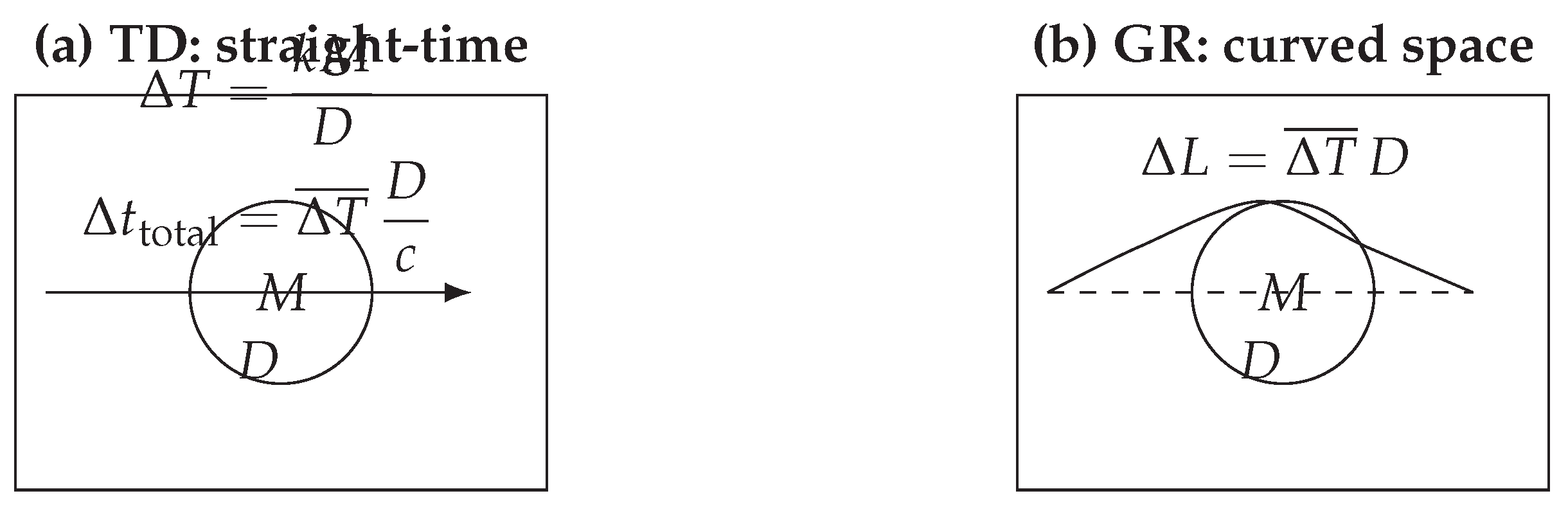

Table 1.
Classic tests in the TD/GR mapping (PPN with ).
| Effect | Prediction |
|---|---|
| Gravitational redshift | |
| Light deflection | |
| Shapiro delay (one way) | |
| Perihelion precession |
Disclaimer/Publisher’s Note: The statements, opinions and data contained in all publications are solely those of the individual author(s) and contributor(s) and not of MDPI and/or the editor(s). MDPI and/or the editor(s) disclaim responsibility for any injury to people or property resulting from any ideas, methods, instructions or products referred to in the content. |
© 2025 by the authors. Licensee MDPI, Basel, Switzerland. This article is an open access article distributed under the terms and conditions of the Creative Commons Attribution (CC BY) license (http://creativecommons.org/licenses/by/4.0/).
Copyright: This open access article is published under a Creative Commons CC BY 4.0 license, which permit the free download, distribution, and reuse, provided that the author and preprint are cited in any reuse.


