
Submitted:
28 August 2025
Posted:
28 August 2025
You are already at the latest version
Abstract
This paper presents the implementation of a nonlinear state observer in real-time applied to an erbium-doped fiber laser system. The observer is designed to estimate population inversion, a state variable that cannot be directly measured due to the physical limitations of the sensing devices. Taking advantage of the fact that laser intensity can be acquired in real time, an observer was developed that reconstructs the dynamics of population inversion from this measurable variable. To validate and reinforce the estimate obtained through the observer, a recurrent wavelet first-order neural network (RWFONN) was implemented, trained to identify both state variables: laser intensity and population inversion. This network efficiently captures the nonlinear dynamic characteristics of the system, complementing the observer’s performance. To evaluate the accuracy and reliability of the results, two metrics were applied: the Euclidean distance and the mean squared error (MSE), both of which confirmed the consistency between the estimated and expected values. The ultimate goal of this research is to establish a neural control architecture that combines the estimation capabilities of state observers with the generalization and modeling power of artificial neural networks. This hybrid approach opens the door to the development of more robust and adaptive control schemes for highly dynamic complex laser systems.
Keywords:
state observer
; erbium-doped fiber laser
; recurrent wavelet first order neural network
1. Introduction
Erbium-doped fiber lasers (EDFLs) have diverse applications in optical communications and photonics. These lasers can be compact and tunable, with one design incorporating a microfiber coupled to a silica microsphere for wavelength tuning and filtering [1]. EDFLs are particularly useful in long-distance communication, amplifying optical signals without conversion to electrical signals [2]. Recent research has focused on producing ultra-short pulse widths and high repetition rates. A tunable EDFL based on random distributed feedback has demonstrated a broad tuning range of 40 nm with a narrow linewidth [3]. A novel configuration called erbium-doped fiber laser amplifier (EDFLA) combines laser and amplifier functionalities, serving as an optical amplifier, laser source, and ON/OFF optical tool [4]. These advancements in EDFL technology contribute to improved performance and versatility in optical communication systems and other photonic applications.
This collection of papers explores various aspects of laser fiber systems and their control. [5] demonstrated an operation state switchable erbium-doped fiber laser, studying pulse-splitting and multi-level modulation. [6] focused on process observation in selective laser melting, developing a variable retro-focus system and real-time signal acquisition for improved manufacturing processes. [7] compared Proportional Integral Derivative (PID) control with Observer-Based State Feedback (OBSF) control for precise laser beam positioning, finding OBSF to be superior in disturbance rejection. [8] introduced a novel approach using principal states of polarization to describe tunability in fiber lasers, validating their method for a 4-m fiber laser over a 2 nm wavelength range. These studies collectively contribute to advancing laser fiber technology, addressing challenges in beam control, process observation, and system tunability across various applications.
Recurrent Wavelet First-Order Neural Networks (RWFONNs) have emerged as powerful tools for real-time identification and control of complex systems. These networks utilize a single-layer, single-neuron structure with a Morlet wavelet activation function [9,10]. RWFONNs have demonstrated effectiveness in identifying and controlling robot manipulators [9] and chaotic systems implemented in Field-Programmable Analog Arrays [10]. Notably, a fixed-parameter RWFONN has shown the ability to identify multiple chaotic systems without recalibration [11]. These networks offer advantages in online training and real-time applications without requiring multiple epochs or data batches [10]. Additionally, first-order recurrent neural networks have been classified hierarchically based on their expressive powers, providing insights into their computational capabilities and attractive behaviors [12].
The integration of artificial neural networks with Luenberger observers has been explored for state estimation in nonlinear and uncertain systems. Recurrent Neural Networks (RNN) have been used to create Luenberger-like observers for discrete-time nonlinear systems with partial information [13]. Extended Luenberger observers have been connected to Grossberg’s additive model for dynamic neural networks, enabling state estimation for systems with partially known or unknown dynamics [14]. A multilayer recurrent neural network has been developed for real-time synthesis of asymptotic state observers in linear time-varying systems [15]. Additionally, robust asymptotic neuro-observers with time delay terms have been designed for unknown nonlinear systems, using dynamic neural networks to estimate unknown dynamics and compensate for differential effects in Luenberger observers [16]. These approaches have demonstrated effectiveness in various applications, including the van der Pol oscillator and robotic systems.
This paper presents the mathematical models of the fiber laser, the state observer, and the artificial neural network in Section 2; the methodology and process description are presented in Section 3; the results obtained from the implementation of the state observer and the RWFONN are presented in Section 4; the discussion is presented in Section 5; and the conclusion of the paper is presented in Section 6.
2. Mathematical Models
This section describes the three mathematical models employed in the proposed implementation: The EDFL model, the State observer model, and the RWFONN model.
2.1. Erbium-Doped Fiber Laser Mathematical Model
The dynamics of a laser operating in a single emission mode can be described by a system of three coupled differential equations, which account for the evolution of the optical field, population inversion, and polarization. Each of these variables relaxes on different time scales. In certain regimes, this difference allows for adiabatic approximations, where one or more variables are considered to evolve instantaneously relative to the others. These approximations simplify the mathematical model by reducing the number of equations needed to describe the system’s behavior.
Depending on the relative relaxation times of these variables, lasers are classified into three categories. In class A lasers, both the population inversion and polarization relax much faster than the optical field, typically resulting in a single stable stationary state. Class B lasers, where only polarization relaxes quickly, can exhibit relaxation oscillations due to energy exchange between the optical field and the inversion. In class C lasers, all three variables relax on comparable time scales, allowing for more complex dynamics, such as sustained oscillations or deterministic chaos. External perturbations—like parameter modulation—can also induce periodic or chaotic behavior in class B lasers, which includes many solid-state and semiconductor devices [17,18,19,20,21].
From a nonlinear dynamics standpoint, fiber lasers doped with rare-earth elements (such as erbium), when subjected to external modulation, are also considered class B systems [22]. In such lasers, the fast-relaxing polarization variable is commonly eliminated via adiabatic approximation, reducing the model to two rate equations: one for the optical field and another for the population inversion. While the nonlinear behavior of lasers has been extensively studied, the analysis of erbium-doped fiber lasers (EDFLs) is a more recent endeavor. Experimental results indicate that EDFLs share the fundamental dynamic traits of class B systems, including the emergence of chaotic regimes [23,24]. Importantly, a more comprehensive model—one that retains all three dynamic variables without adiabatic simplifications—has been developed and validated in prior studies. This full model enables a more accurate representation of transient phenomena, nonlinear interactions, and complex behaviors such as self-pulsing, self-modulation, and chaos induced by internal or external perturbations [25].
2.1.1. Normalized Equations of EDFL
To achieve a synthesis and generalization of the laser model, the complete system was transformed into the following compact form
the system can be expressed in vector notation as
where
wich can be rewritten as
where

Table 1.
Table of parameters and values of the Normalized Equations.
| Parameters and values | Parameters and values |
|---|---|
The variable x represents the normalized laser intensity, while y corresponds to the population inversion. The parameter denotes the pump power, and the pump modulation, .
2.2. Mathematical Model of State Observer
In dynamic systems, particularly those of a non-linear nature, direct access to all state variables is often impractical due to physical, technological, or cost constraints on instrumentation. Given this limitation, nonlinear state observers are essential tools for the real-time estimation of non-measurable variables. For the construction of the state observer, we define the state vector and the input, taking as reference the equation (3)
Since the system contains non-linear terms such as , it is generally represented as a non-linear system
where
So the complete system is expressed as
The output of the system is defined as
For the construction of the state observer, we define the vectors
where and are gains of the observer. Then, the non-linear observer can be expressed as
where is named the estimated error. The estimated output is
In this work, a state observer has been designed to estimate the state variable corresponding to the population inversion (y). This decision is due to the impossibility of measuring this variable directly in real time and to the lack of adequate electronic instrumentation for its acquisition. The stability analysis of the proposed observer is presented in the Appendix A.
2.3. Mathematical Model of RWFONN
In the present work, a Recurrent Wavelet First-Order Neural Network (RWFONN) was adopted due to its advantageous characteristics over other neural network architectures commonly used in nonlinear system identification. One of the main reasons for this selection lies in its capacity to estimate the internal states of the dynamic system in real time, using an adaptive mechanism that updates its synaptic weights online based on the filtered estimation error. This feature makes the RWFONN particularly suitable for observer-based architectures in systems where certain internal variables, such as population inversion in EDFL, cannot be measured directly. In addition, its wavelet-based structure enables a compact representation of the signal with strong time-frequency localization, improving the network’s generalizability and convergence speed. Compared to more complex models such as the Recurrent High-Order Neural Network (RHONN) or the Recurrent Sigmoid First-Order Neural Network (RSFONN), the RWFONN exhibits a simpler architecture with reduced computational burden, making it more practical for real-time control applications and hardware-limited environments.
In [32], the authors identified a dynamical UDS type I by numerical approximation using an RWFONN, where the general structure is as follows:
where , are the states of the i-th neuron. for is part of the underlying network architecture and will remain fixed during the training process. is the k-th adjustable synaptic weight connecting the j-th state to the i-th neuron, and is a Morlet wavelet activation function defined by , where is the state of the original system to identify; the parameters and are the expansion and dilation terms. The system given in (3) is identified online using RWFONN, with synaptic weights adjusted via the filtered error algorithm. A more detailed description of the network structure can be reviewed in [10] and [25].
3. Methodology and Description of the Process
3.1. Experimental Setup
Figure 1 shows the experimental configuration of the Erbium-Doped Fiber Laser (EDFL). The cavity, with a total length of 6.5 m, includes a 70 cm segment of Erbium-Doped Fiber (Thorlabs, SM-EDF-7/125) with a core diameter of 2.7 m. The EDF is optically pumped by a 977 nm laser diode (LD-BL976PAG500, Thorlabs), whose current is regulated by a Laser Diode Controller (LDC-ITC510, Thorlabs) that also ensures thermal stabilization of the pump source. The pump current is modulated using a sinusoidal signal generated by a waveform generator (WFG-AFG3102, Tektronix), which is connected to the modulation input of the LDC. The optical signal from the LD passes through a Polarization Controller (Thorlabs, FPC020) and is injected into the cavity via a Wavelength Division Multiplexer (WDM-WD9850FD, Tektronix). The resonator comprises two Fiber Bragg Gratings (FBG1 and FBG2, Thorlabs), centered at 1550 nm, with reflectivities of 100% and 95.88%, respectively. The cavity also includes an Optical Isolator (Thorlabs, IO-H-1550APC) at the FBG2 port to eliminate back-reflections. The output laser signal from the FBG2 port is detected by a photodiode (PD2, Thorlabs PDA10CS-AC), and the resulting electrical signal is digitized through a data acquisition card DAC (dSPACE DS1104). The sampled signal is processed by a nonlinear state observer (see SubSection 2.2), as explained in the following SubSection 3.2, which estimates non-measurable internal states such as population inversion. This observer also enables comparison between experimental and numerically reconstructed signals and can optionally generate feedback to the modulation input via the WFG-LDC interface. All optical components are based on single-mode fiber (SMF-28, Thorlabs) with a cladding diameter of 200 m. During all measurements, the EDFL system was maintained under active thermal stabilization.
3.2. Schematic Implementation of State Observer in Real-Time
Figure 2 shows the real-time schematic of the implementation of the nonlinear state observer applied to the EDFL system. The diagram consists of three main processes. The first block, labeled EDFL experimental system, represents the physical laser setup, from which the laser intensity x is measured and sent to the observer. In the second block, labeled State observer, a nonlinear observer estimates both the measured variable and reconstructs the unmeasured internal state , which corresponds to population inversion. The observer dynamics are governed by a system of differential equations shown within the block, and the error between the measured and estimated outputs drives the estimation.
These estimated states () are then input to the third block, RWFONN, which performs system identification by generating outputs and based on the neural model. Additionally, the diagram includes error signals , , and , which quantify the estimation and identification accuracy by comparing observed, estimated, and neural network outputs.
3.3. Temporary Rescaling
Since the integration step size for numerically solving the differential equations describing the observer dynamics implemented in Simulink is very small compared to the sampling rate of the real-time DAC, the observer equation is temporarily rescaled as follows: If we consider with , where H is the scale parameter of the observer, the equation changes to
by multiplying equations (11) and (12) by H, these become
Setting the parameter H to a suitable value allows the observer model implemented in Simulink and the real-time acquisition platform to work in real time with the DAC.
4. Real-Time Observer and Neural Identification Results
To evaluate the performance and practical viability of the proposed nonlinear state observer, the system was implemented in real time, incorporating the RWFONN for state reconstruction. This section presents the experimental results obtained from a setup based on an erbium-doped fiber laser, where direct measurement of critical internal states, such as population inversion, is not feasible. The observer was designed to estimate these non-measurable variables from the measured laser intensity, and the RWFONN was trained online using the filtered estimation error to adaptively improve the accuracy of the reconstruction. The following results demonstrate the effectiveness of the proposed architecture under varying operating conditions, highlighting its convergence behavior, robustness against unmodeled dynamics, and suitability for real-time control scenarios.
The structure of the artificial neural network used to carry out the identification of the state variables obtained through the state observer is the following
The state vector
the system matrix, which contains the linear coefficients of the variables and , is defined as
the vector of wavelet activation functions evaluated is
the weighted parameters for each nonlinear input are grouped into the following vector
Finally, the external input to the system is represented as
Then, the equations can be written in matrix form as
where ∘ represents the element-by-element product.
Table 3.
Parameters of the state observer and RWFONN.
| Parameters | Parameters |
|---|---|
Figure 3 presents the laser intensity and reconstructed population inversion of an EDFL under three distinct initial conditions in each row. These conditions arise from independent experimental acquisitions at 80kHz, where the measurement system, comprising the photo-detector, DAC, and computer, was reinitialized before each run. This variability tests the robustness of the proposed estimation framework. The left column [a)–c)] presents the laser intensity signals: experimental measurements (red dashed line), estimates from the nonlinear state observer (blue continuous line), and predictions by a RWFONN (black dashed line). The right column [d)–f)] shows the corresponding reconstructions of the nonmeasurable state variable, the population inversion, obtained from both the observer (red dashed line) and the neural network (black continuous line). The consistent agreement between the observer and neural network across all three initial conditions confirms the effectiveness and repeatability of the hybrid approach for real-time state reconstruction in complex EDFL systems.
Figure 4 show the results of the real-time observer and identification of the Laser Intensity. The results shown in the graphs were obtained for different frequency values. For this study, the frequencies of interest were considered to be every 10kHz. The efficiency of the observer and the artificial neural network is indicated in achieving both estimation and identification. Each figure shows a box with detail, in which good estimation and identification of laser intensity can be observed.
Figure 5 shows the results of the estimated population inversion and neural identification. In the same way as for the laser intensity graphs, the results shown in the graphs were obtained for different frequency values. The frequencies of interest were considered to be every 10kHz. The efficiency of the observer and the artificial neural network is indicated in achieving both estimation and identification. Each figure shows a box with detail, in which good estimation and identification of population inversion can be observed.
4.1. Euclidean Distance and MSE Metrics
Two metrics were employed to quantitatively validate the accuracy of the proposed state observer and the implemented artificial neural network: Euclidean distance [33] and mean square error (MSE). These metrics allow for the comparison of the behavior of observed and estimated variables concerning simulated or measured references, offering an objective criterion for evaluating system performance. Specifically, the Euclidean distance between the trajectories of the estimated and actual variables was calculated, and MSE was used to measure the level of error dispersion over time. These analytical tools were applied to different pairs of relevant system variables, which allowed identifying the degree of agreement and reliability of the proposed model in estimating variables that cannot be directly measured.
Figure 6.
Euclidean distance metric to 80kHz value of frequency. Difference between: a) laser intensity and the first variable estimated by the state observer , b) laser intensity and first variable of the RWFONN , and c) second variable estimated by the state observer and the second variable of the RWFONN .
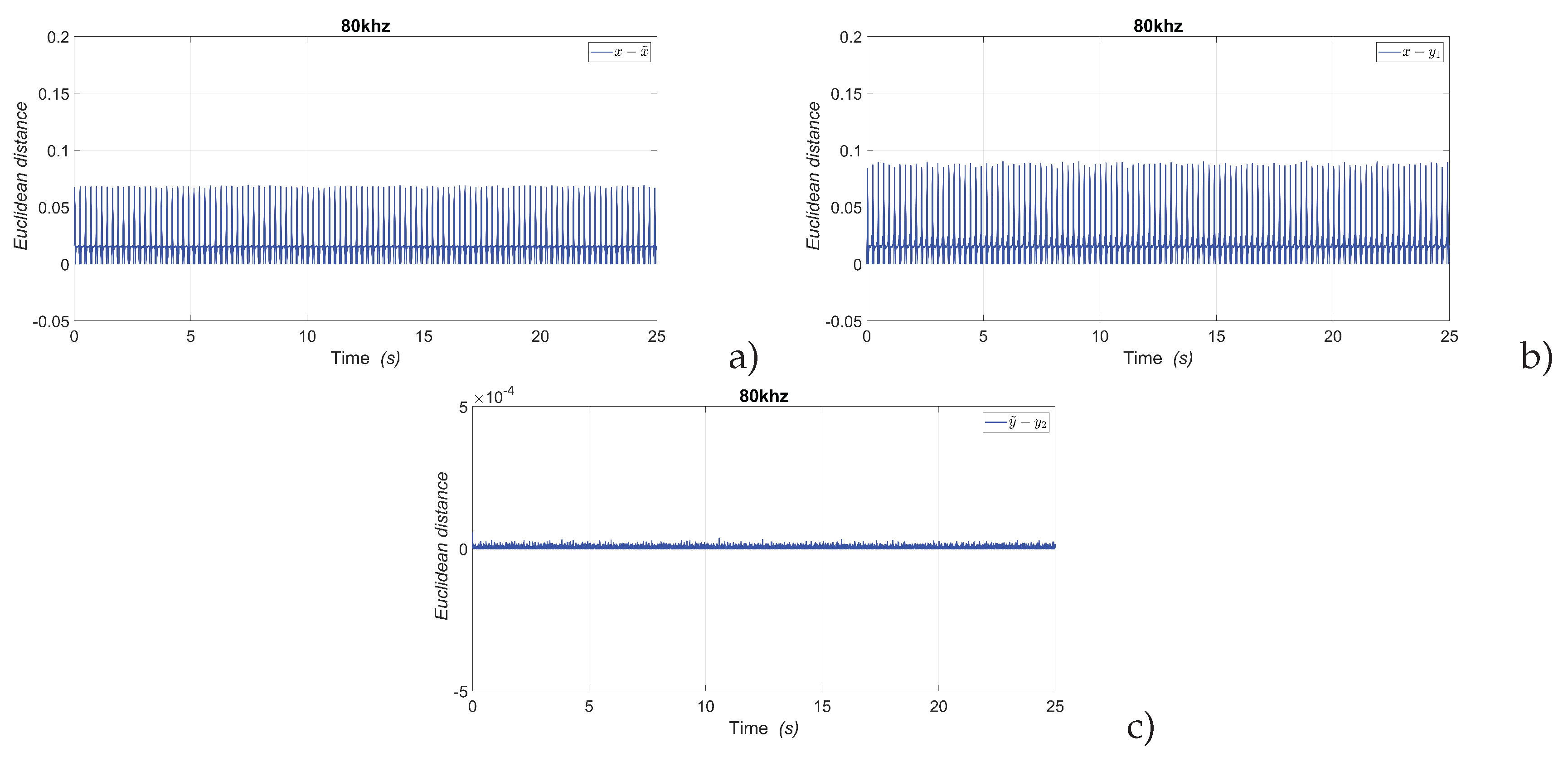
To check the accuracy of the estimates under steady-state conditions, the selected metrics were applied to the case where the input signal to the system was 80kHz. In this scenario, three specific combinations were compared: the difference between the real laser intensity and observed state , the difference between the real laser intensity and the first variable of neural network , and finally, the difference between the variable estimated by the state observer and the second variable of neural network . In all three scenarios, it can be observed that the error is close to zero, and this guarantees good observation and identification of the laser system.
The results obtained from Table 4, calculating the mean square error for each frequency value evaluated show values consistently close to zero. This trend indicates a high accuracy of the proposed state observer, since the difference between the estimated and actual signals is minimal throughout the operating range. Consequently, the correct reconstruction of the non-measurable variable and the adequate identification of the system’s dynamic behavior are confirmed. These results support the reliability of the approach adopted for real-time estimation within the EDFL.
5. Discussion
The implementation of the proposed state observer demonstrates the feasibility of estimating the population inversion in an erbium-doped laser fiber. This variable cannot be directly measured due to the physical limitations of the system. The estimation was based on the measurement of the laser output intensity, allowing the complete dynamics of the system to be inferred with an acceptable margin of error. This strategy represents an efficient alternative for monitoring internal variables in complex optical systems, without the need to modify their physical architecture or interrupt their operation.
The incorporation of an artificial neural network allowed the behavior estimated by the observer to be validated, showing a significant correlation between the two methods. Furthermore, the ANN proved capable of capturing nonlinearities inherent to the system, suggesting its usefulness as a backup or support under more demanding operating conditions or when faced with variations in the laser’s physical parameters.
An important observation is that, while the state observer offers a more transparent solution from a physical and mathematical perspective, the neural network provides flexibility and generalization capabilities when sufficient training data are available. However, its performance depends heavily on the quality of the data and the selected architecture.
Overall, the combination of both methodologies not only improves the robustness of the estimation system but also opens the possibility of designing more advanced hybrid strategies for controlling and monitoring laser systems. This research lays the groundwork for future real-time implementations in more complex experimental setups.
6. Conclusions
The results obtained in this work demonstrate the effectiveness of the proposed state observer, in conjunction with the RWFONN, for the estimation and reconstruction of internal variables in an erbium-doped laser system. In particular, the second state variable, which cannot be directly measured due to the system’s physical limitations, was estimated in real time. Furthermore, both observed state variables were accurately identified, validating the proposed scheme’s ability to represent system dynamics robustly and adaptively. This approach not only reduces the need for invasive or expensive instrumentation but also lays the groundwork for the design of future advanced control schemes in nonlinear optical systems. The RWFONN structure, with its online learning and low computational cost, proved particularly well-suited for real-time applications where efficiency and accuracy are critical.
Author Contributions
D.A.M.G.: Conceptualization, Investigation, Methodology, Validation, Writing—Original Draft, Writing—Review, and Editing. D.L.M.: Conceptualization, Methodology, Validation, Writing—Review, and Editing. R.J.R.: Validation, Writing—Review, and Editing. J.H.G.L.: Methodology, Validation, Writing—Original Draft, Writing—Review, and Editing. G.H.C.: Validation, Writing—Review, and Editing. L.J.O.G.: Validation, Writing—Review, and Editing. All authors have read and agreed to the published version of the manuscript.
Data Availability Statement
The data related to the paper are available from the corresponding authors upon reasonable request.
Acknowledgments
D.A.M.G. acknowledges the support of SECIHTI, which received an academic postdoctoral fellowship with application number: 2290436. L.J.O.G. Thanks to the Potosino Council of Science and Technology (COPOCYT) for the support in Trust project 23871 of the 2023-01 Call.
Conflicts of Interest
The authors declare no conflict of interest.
Appendix A Stability analysis
Analyzing the stability of the error system between the original laser ( Equation (6)) and the state observer (Equation (8)), the representation in terms of the dynamic estimated error is defined as follows
Reducing and factoring, the Equation (A1) can be rewritten as follows
The next positive definite Lyapunov function guarantees that the error tends to zero
once that the derivative of the Lyapunov function become
On the other hand, Equation (A4) can be written in matrix form, to find the values of and to find the optimal gains that guarantee the stability of the complete system
in the form , with 0, if
and
References
- Sulaiman, A.; Harun, S.W.; Ahmad, H. Erbium-doped fiber laser with a microfiber coupled to silica microsphere. IEEE Photonics Journal 2012, 4, 1065–1070. [Google Scholar] [CrossRef]
- Subramaniam, T.K. Erbium doped fiber lasers for long distance communication using network of fiber optics. Am. J. Opt. Photonics 2015, 3, 34. [Google Scholar] [CrossRef]
- Wang, Y.; Suzek, T.; Zhang, J.; Wang, J.; He, S.; Cheng, T.; Shoemaker, B.A.; Gindulyte, A.; Bryant, S.H. PubChem bioassay: 2014 update. Nucleic acids research 2014, 42, D1075–D1082. [Google Scholar] [CrossRef]
- Bouzid, B. Erbium Doped Fiber Laser and Amplifier. Optics and Photonics Journal 2014, 2014. [Google Scholar] [CrossRef]
- Lin, K.H.; Kang, J.J.; Wu, H.H.; Lee, C.K.; Lin, G.R. Manipulation of operation states by polarization control in an erbium-doped fiber laser with a hybrid saturable absorber. Optics express 2009, 17, 4806–4814. [Google Scholar] [CrossRef]
- Thombansen, U.; Gatej, A.; Pereira, M. Process observation in fiber laser–based selective laser melting. Optical engineering 2015, 54, 011008–011008. [Google Scholar] [CrossRef]
- Konadu, K.A.; Yi, S.; Choi, W.; Abu-Lebdeh, T. Robust positioning of laser beams using proportional integral derivative and based observer-feedback control. American Journal of Applied Sciences 2013, 10, 374. [Google Scholar] [CrossRef]
- Friedman, N.; Geiger, D.; Goldszmidt, M. Bayesian network classifiers. Machine learning 1997, 29, 131–163. [Google Scholar] [CrossRef]
- Vázquez, L.A.; Jurado, F. Continuous-time decentralized wavelet neural control for a 2 DOF robot manipulator. In Proceedings of the 2014 11th International Conference on Electrical Engineering, Computing Science and Automatic Control (CCE). IEEE; 2014; pp. 1–6. [Google Scholar]
- Magallón-García, D.; García-López, J.; Huerta-Cuellar, G.; Jaimes-Reátegui, R.; Diaz-Diaz, I.; Ontanon-Garcia, L. Real-time neural identification using a recurrent wavelet first-order neural network of a chaotic system implemented in an FPAA. Integration 2024, 96, 102134. [Google Scholar] [CrossRef]
- Echenausía-Monroy, J.L.; Pena Ramirez, J.; Álvarez, J.; Rivera-Rodríguez, R.; Ontañón-García, L.J.; Magallón-García, D.A. A recurrent neural network for identifying multiple chaotic systems. Mathematics 2024, 12, 1835. [Google Scholar] [CrossRef]
- Cabessa, J.; Villa, A.E. A hierarchical classification of first-order recurrent neural networks. In Proceedings of the International Conference on Language and Automata Theory and Applications. Springer; 2010; pp. 142–153. [Google Scholar]
- Salgado, I.; Chairez, I. Nonlinear discrete time neural network observer. Neurocomputing 2013, 101, 73–81. [Google Scholar] [CrossRef]
- Erdogmus, D.; Genç, A.U.; Príncipe, J.C. A neural network perspective to extended Luenberger observers. Measurement and Control 2002, 35, 10–16. [Google Scholar] [CrossRef]
- Wang, J.; Wu, G. A multilayer recurrent neural network for on-line synthesis of minimum-norm linear feedback control systems via pole assignment. Automatica 1996, 32, 435–442. [Google Scholar] [CrossRef]
- Yu, W.; Poznyak, A.S. Robust Asymptotic Neuro Observer with Time Delay Term. submitted to CDC, 99.
- Fischer, I.; Liu, Y.; Davis, P. Synchronization of chaotic semiconductor laser dynamics on subnanosecond time scales and its potential for chaos communication. Physical Review A 2000, 62, 011801. [Google Scholar] [CrossRef]
- Vanwiggeren, G.D.; Roy, R. Communication with chaotic lasers. Science 1998, 279, 1198–1200. [Google Scholar] [CrossRef]
- Donati, S.; Mirasso, C.R. Introduction to the feature section on optical chaos and applications to cryptography. IEEE Journal of Quantum Electronics 2002, 38, 1138–1140. [Google Scholar] [CrossRef]
- Ohtsubo, J.; Davis, P. Chaotic optical communication. Unlocking Dynamical Diversity: Optical Feedback Effects on Semiconductor Lasers, 2005; 307–334. [Google Scholar]
- Soriano, M.C.; Ruiz-Oliveras, F.; Colet, P.; Mirasso, C.R. Synchronization properties of coupled semiconductor lasers subject to filtered optical feedback. Physical Review E 2008, 78, 046218. [Google Scholar] [CrossRef]
- Arecchi, F.T.; Harrison, R.G. Instabilities and chaos in quantum optics; Vol. 34, Springer Science & Business Media, 2012.
- Lacot, E.; Stoeckel, F.; Chenevier, M. Dynamics of an erbium-doped fiber laser. Physical Review A 1994, 49, 3997. [Google Scholar] [CrossRef]
- Tehranchi, A.; Kashyap, R. Extremely efficient DFB lasers with flat-top intra-cavity power distribution in highly erbium-doped fibers. Sensors 2023, 23, 1398. [Google Scholar] [CrossRef]
- Magallón-García, D.A.; López-Mancilla, D.; Jaimes-Reátegui, R.; García-López, J.H.; Huerta Cuellar, G.; Ontañon-García, L.J.; Soto-Casillas, F. Experimental State Observer of the Population Inversion of a Multistable Erbium-Doped Fiber Laser. In Proceedings of the Photonics. MDPI, Vol. 11; 2024; p. 951. [Google Scholar]
- Pisarchik, A.N.; Kir’yanov, A.V.; Barmenkov, Y.O.; Jaimes-Reátegui, R. Dynamics of an erbium-doped fiber laser with pump modulation: theory and experiment. Journal of the Optical Society of America B 2005, 22, 2107–2114. [Google Scholar] [CrossRef]
- Pisarchik, A.N.; Jaimes-Reátegui, R.; Sevilla-Escoboza, R.; Huerta-Cuellar, G.; Taki, M. Rogue waves in a multistable system. Physical Review Letters 2011, 107, 274101. [Google Scholar] [CrossRef]
- Sevilla-Escoboza, R.; Pisarchik, A.N.; Jaimes-Reátegui, R.; Huerta-Cuellar, G. Selective monostability in multi-stable systems. Proceedings of the Royal Society A: Mathematical, Physical and Engineering Sciences 2015, 471, 20150005. [Google Scholar] [CrossRef]
- Pisarchik, A.; Jaimes-Reátegui, R.; Sevilla-Escoboza, R.; Huerta-Cuellar, G. Multistate intermittency and extreme pulses in a fiber laser. Physical Review E—Statistical, Nonlinear, and Soft Matter Physics 2012, 86, 056219. [Google Scholar] [CrossRef] [PubMed]
- Huerta-Cuellar, G.; Pisarchik, A.N.; Barmenkov, Y.O. Experimental characterization of hopping dynamics in a multistable fiber laser. Physical Review E—Statistical, Nonlinear, and Soft Matter Physics 2008, 78, 035202. [Google Scholar] [CrossRef] [PubMed]
- Reategui, R.J. Dynamic of complex systems with parametric modulation: duffing oscillators and a fiber laser. PhD thesis, Centro de Investigaciones en Optica Leon, Mexico, 2004.
- Magallón-García, D.A.; Ontanon-Garcia, L.J.; García-López, J.H.; Huerta-Cuéllar, G.; Soubervielle-Montalvo, C. Identification of chaotic dynamics in jerky-based systems by recurrent wavelet first-order neural networks with a morlet wavelet activation function. Axioms 2023, 12, 200. [Google Scholar] [CrossRef]
- Liberti, L.; Lavor, C.; Maculan, N.; Mucherino, A. Euclidean distance geometry and applications. SIAM review 2014, 56, 3–69. [Google Scholar] [CrossRef]
Figure 1.
Experimental setup of the EDFL system. The output intensity is acquired and processed by a nonlinear observer that estimates the state of the population inversion. The observer compares experimental and numerical intensity for real-time analysis.
Figure 1.
Experimental setup of the EDFL system. The output intensity is acquired and processed by a nonlinear observer that estimates the state of the population inversion. The observer compares experimental and numerical intensity for real-time analysis.
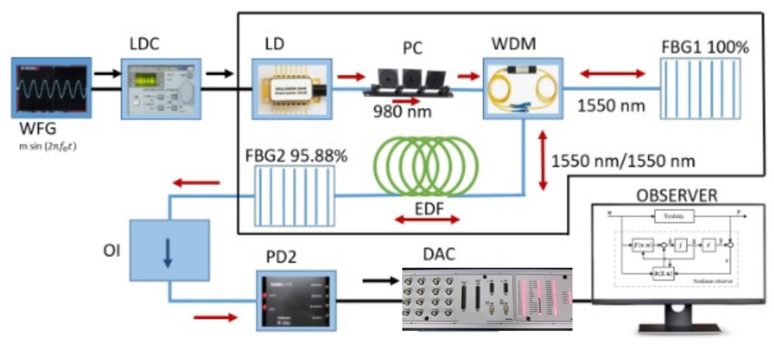
Figure 2.
Schematic implementation of the nonlinear observer for the EDFL system. The observer estimates laser intensity and reconstructs population inversion in real time. A neural network (RWFONN) validates the observer’s performance using the estimated states.
Figure 2.
Schematic implementation of the nonlinear observer for the EDFL system. The observer estimates laser intensity and reconstructs population inversion in real time. A neural network (RWFONN) validates the observer’s performance using the estimated states.
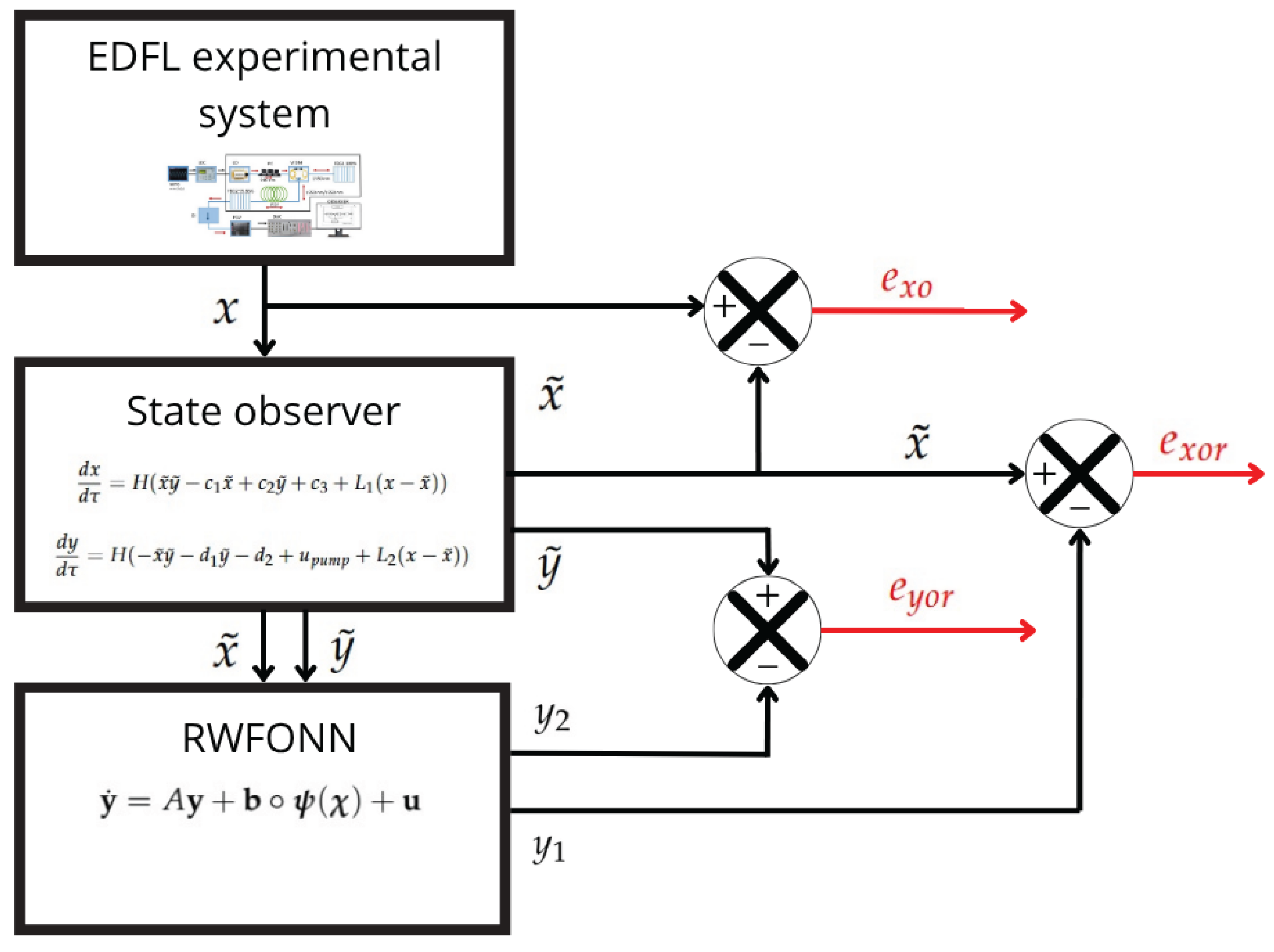
Figure 3.
Laser intensity and population inversion estimations for an EDFL. Left column [a)–c)] shows experimental laser intensity (red dashed line), observer estimate (blue continuous line), and RWFONN output (black dashed line). Right column [d)–f)] shows population inversion estimated by the observer (red dashed line) and RWFONN (black continuous line). Each row corresponds to different initial conditions from the acquisition system.
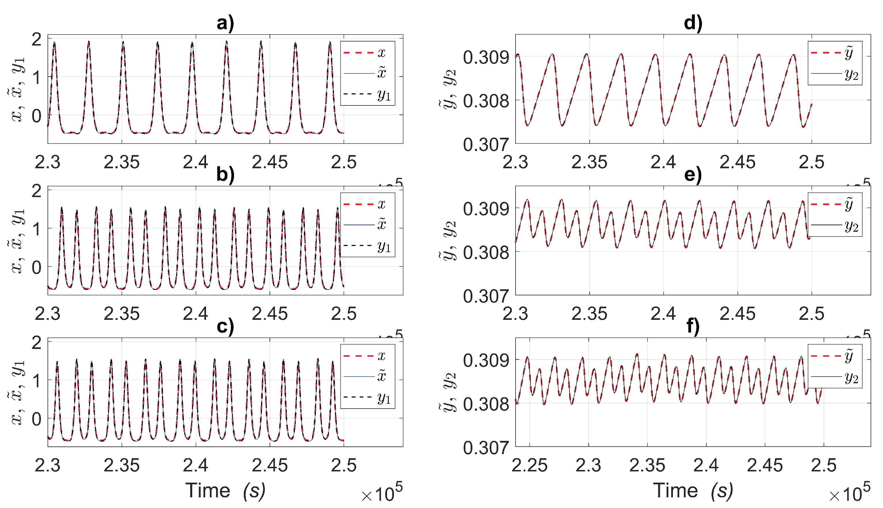
Figure 4.
Real laser intensity (red dashed line), state observer (blue solid line), and artificial neural network (blue solid line), respectively, for every value of frequency.
Figure 4.
Real laser intensity (red dashed line), state observer (blue solid line), and artificial neural network (blue solid line), respectively, for every value of frequency.
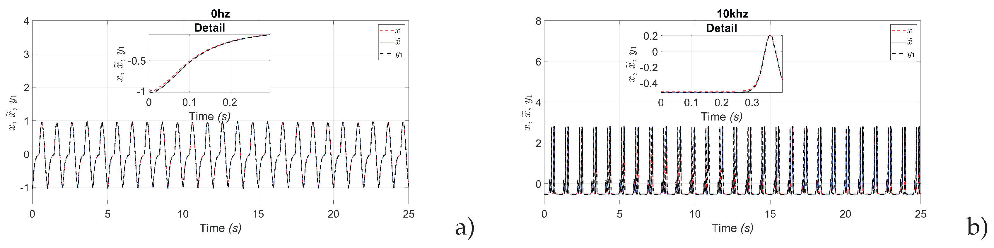
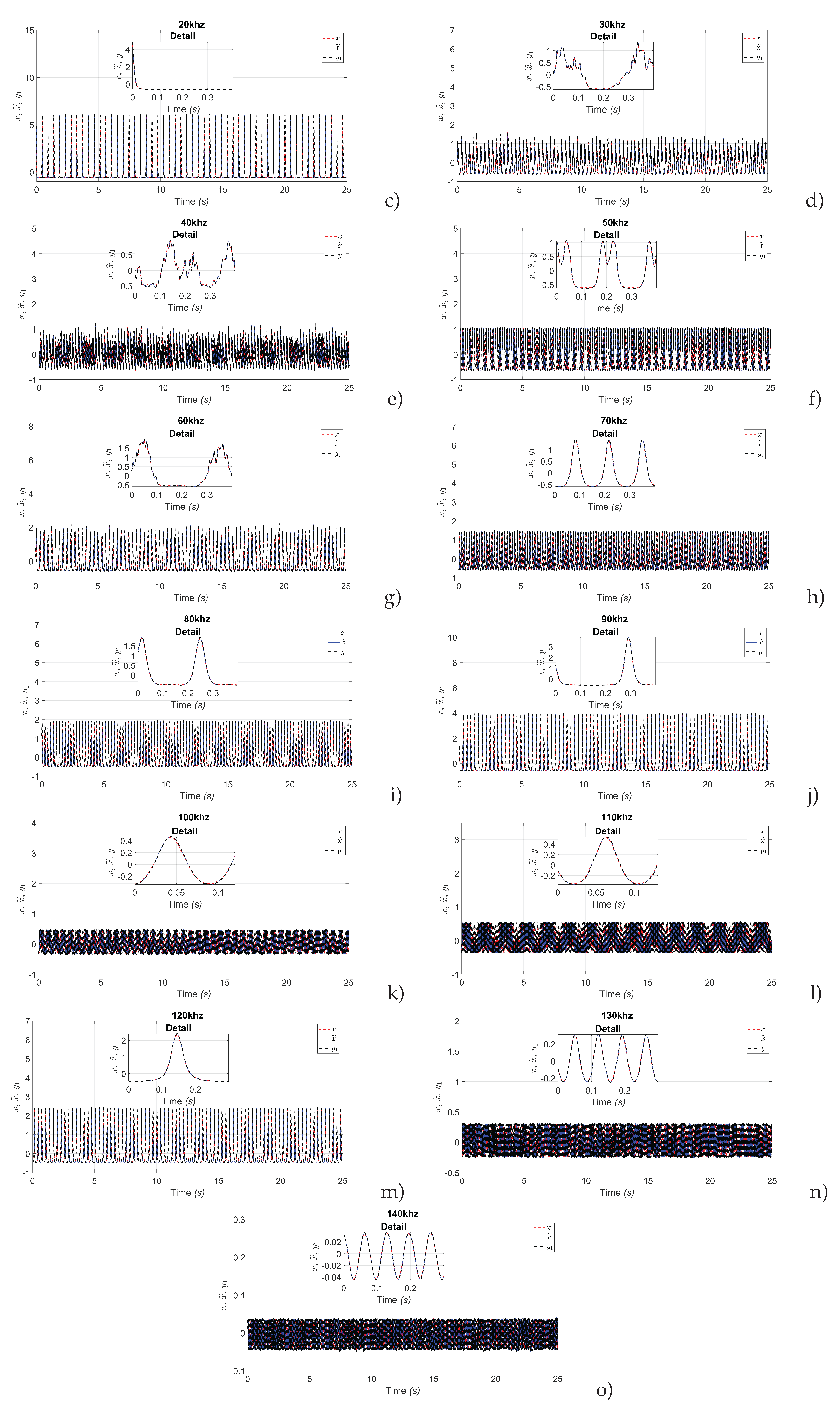
Figure 5.
Population inversion estimated (red dashed line), artificial neural network (black solid line), respectively, for every value of frequency.
Figure 5.
Population inversion estimated (red dashed line), artificial neural network (black solid line), respectively, for every value of frequency.
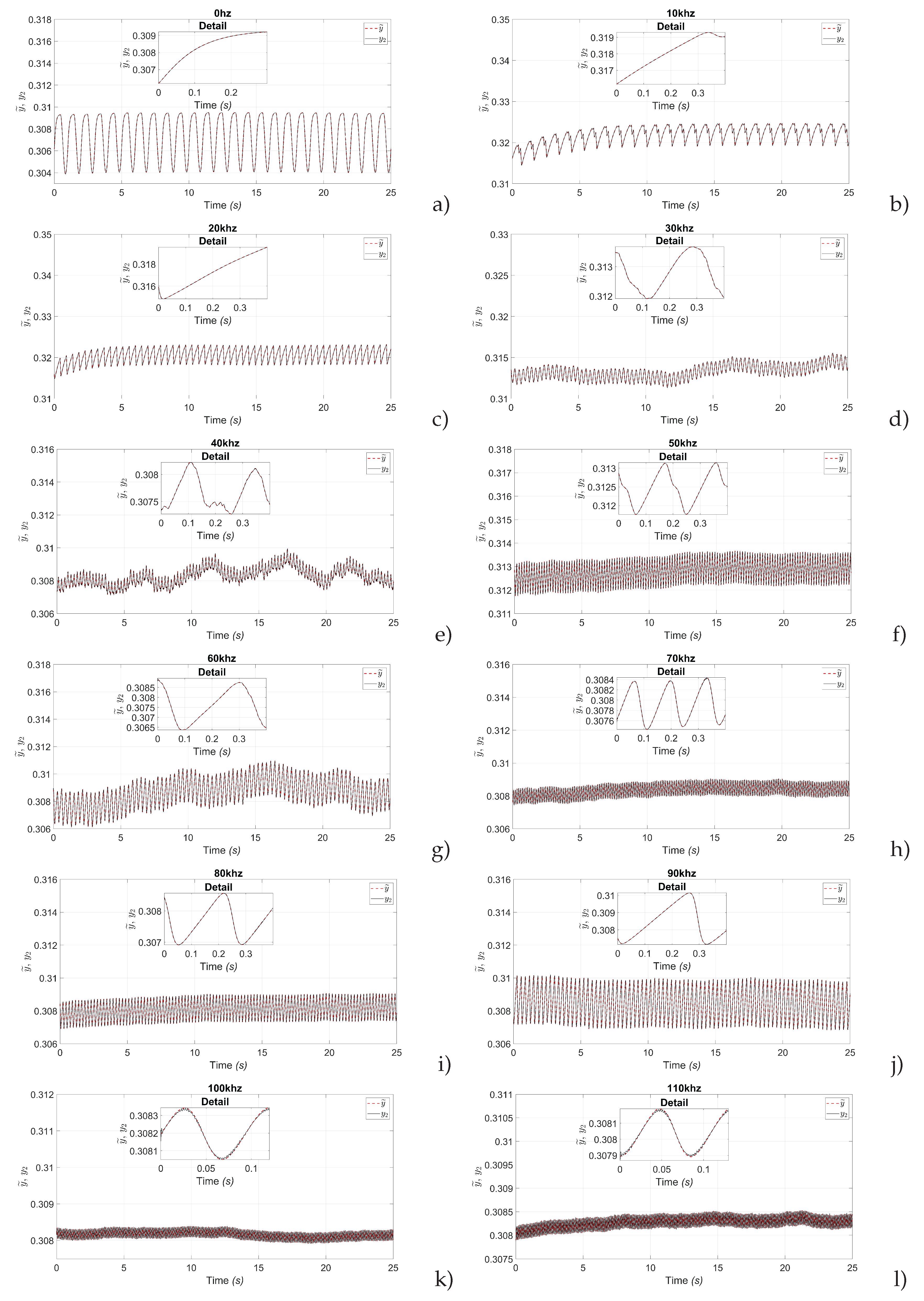
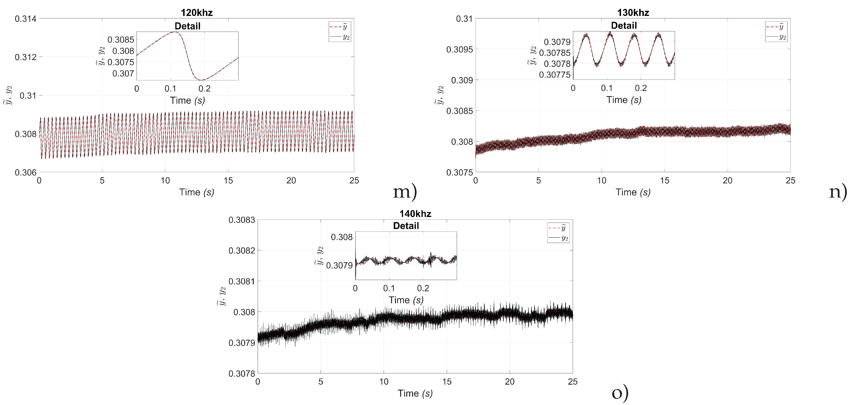
Table 4.
MSE for every value of frequency.
| Frequency | |||
|---|---|---|---|
| 10kHz | 10.0 | 20.0 | 1.008 |
| 20kHz | 30.0 | 50.0 | 2.449 |
| 30kHz | 3.91 | 7.71 | 0.412 |
| 40kHz | 3.25 | 10.0 | 0.265 |
| 50kHz | 5.23 | 9.51 | 0.521 |
| 60kHz | 7.11 | 10.0 | 0.701 |
| 70kHz | 5.81 | 10.0 | 0.565 |
| 80kHz | 6.31 | 9.33 | 0.652 |
| 90kHz | 10.0 | 20.0 | 1.426 |
| 100kHz | 1.06 | 2.13 | 0.177 |
| 110kHz | 1.42 | 3.10 | 0.200 |
| 120kHz | 7.05 | 10.0 | 0.725 |
| 130kHz | 0.56 | 1.36 | 0.135 |
| 140kHz | 0.01 | 0.03 | 0.097 |
Disclaimer/Publisher’s Note: The statements, opinions and data contained in all publications are solely those of the individual author(s) and contributor(s) and not of MDPI and/or the editor(s). MDPI and/or the editor(s) disclaim responsibility for any injury to people or property resulting from any ideas, methods, instructions or products referred to in the content. |
© 2025 by the authors. Licensee MDPI, Basel, Switzerland. This article is an open access article distributed under the terms and conditions of the Creative Commons Attribution (CC BY) license (http://creativecommons.org/licenses/by/4.0/).
Copyright: This open access article is published under a Creative Commons CC BY 4.0 license, which permit the free download, distribution, and reuse, provided that the author and preprint are cited in any reuse.


