Functional Nonparametric Estimation of a Conditional Distribution Function under Spatial Weak Dependence

1. Introduction

In recent years, the field of statistical analysis has witnessed significant advancements, particularly in the context of dependent data. This evolution is evident in a variety of groundbreaking studies that have contributed to our understanding and methodologies [1]. Functional Data Analysis (FDA) is a statistical method that is used to analyze data that are considered functions, rather than just single values.

In traditional data analysis, observations are typically represented by single values such as numbers or categories. However, in many scenarios, data are collected over a continuum, such as time, space, or another ordered domain. FDA treats these data as continuous functions or curves rather than discrete points (for an example, see [2,3,4]).

Association refers to the relationship or connection between different elements within a dataset. In statistical analysis and data science, the association between variables and associated data is fundamental to understanding relationships and patterns within data sets. Associations help to explore how changes in one variable may impact another or how variables relate to each other in a dataset. By exploring associations, analysts and researchers can gain insight into how different variables interact and influence each other, leading to informed decision-making and a deeper understanding of the underlying phenomena represented by the data.

Newman’s early work in 1984 set the foundation by exploring the role of research within this domain. The concept of weak dependence, pivotal in this field, was further elaborated by Doukhan and Louhichi in 1999, providing a new perspective on dependence conditions and their applications to moment inequalities [5].

Studies addressing both positive and negative dependent random variables have been explored in various references [6,7,8]. In their work [9], the authors introduced the concept of quasi-association to analyze stochastic occurrences with real values, illustrating the notion of weak dependence. The idea, which is elaborated on by the work mentioned in [10], offers a unified framework for evaluating groups of randomly dependent variables that are positively or negatively dependent. This framework is applicable to the domain of real-valued random fields.

In the corpus of research that is currently available, the approach of nonparametric estimation of quasi-associated random variables has only attracted a small amount of attention. The research conducted by [11] focuses on a limit theorem that pertains to quasi-associated Hilbertian random variables. This theoretical framework was the topic of the examination. Furthermore, in circumstances where dependency is weak, the asymptotic outcomes of an M-estimator of regression are explored according to the findings of [12]. In the research work that is referred to as [13], the asymptotic normality of an estimator is investigated, with particular emphasis placed on the single-index structure of the conditional hazard function.

One of the areas that was considered significant in the study presented in [14,15] was the examination of nonparametric estimation for linked random variables. This was the topic of the work mentioned in [16]. The authors demonstrate the resilient uniform consistency properties of the partial derivatives of multivariate density functions under weak dependency using the approach provided in [17]. In addition to this, they determine the necessary rates of convergence in order to demonstrate the asymptotic normality of these estimators. Regarding the most recent research on quasi-associated data, the work has been carried out by [18,19,20].

In the context of a single-index regression model, the objective of this study is to evaluate the application of the kernel (k-nn) technique, especially in circumstances in which the explanatory variable is measured in functional space. The implementation of this method in circumstances that include association dependency is another aspect that is investigated in this work. The research given in [21] is an investigation of the use of k-nn in a regression model using a single index. This work follows a similar line of thought. Specifically, the study focuses on situations that include functional predictors and it reveals that almost ideal rates of convergence may be attained even in situations where there is an absence of strong reliance.

The purpose of the work mentioned in [22] is to identify the asymptotic characteristic of nonparametric estimation strategies for the regression function in the single functional index model (SFIM), with the assumption of quasi-association dependence.

In addition, the progress of this topic is characterized by the investigation of limit theorems for quasi-associated variables, as Douge’s paper from 2010 [11] demonstrates. Significant advances were made in 2016 with the work that Mechab and Laksaci did on nonparametric relative regression for associated random variables [23]. Daoudi et al. further advanced of research by establishing the asymptotic normality of the estimator of conditional hazard functions in the context of quasi-associated data [24].

In the realm of kernel density estimation on random fields, Lanh.Tat. Tran’s 1990 work was seminal [25], followed by significant contributions by Dabo-Niang and Yao in 2007 and Carbon, Francq and Tran in the same year [26,27]. J. Li and L.T. Tran in 2009 on nonparametric estimation of conditional expectation further underscores the evolving nature of statistical methods and their applications [28].

Moreover, the introduction of kernel nearest neighbors (k-nn) methodologies and the concept of a single functional index have further enriched the landscape of statistical analysis [29]. These approaches offer robust solutions for dealing with various types of data, including those that exhibit complex dependencies. The single functional index approach introduces an efficient way to model the influence of predictor variables on a response variable, simplifying complex multivariate relationships in a more manageable form [30]. This innovation has been instrumental in the advancement of the field, allowing for a more refined and insightful analysis of dependent data.

The integration of these advanced methodologies has opened new avenues in the realm of statistical analysis, particularly in the handling of complex datasets [29,30]. The k-nn approach adapts to the local structure of the data, providing a more accurate representation of the underlying relationships, which is crucial in various fields like finance, healthcare and environmental studies.

Spatial variables and spatial data play a critical role in understanding and analyzing geographic phenomena, patterns, and the development of predictive models and simulations to predict spatial patterns, trends, and future scenarios. Spatial data consists of information that is explicitly tied to geographic locations or coordinates on the Earth’s surface or in a specified area. Spatial data can be represented in various formats, including points, lines, polygons, grids, and rasters. It encompasses both the spatial coordinates and associated attribute data.

Using spatial data analysis techniques, researchers, policymakers, and practitioners can gain valuable insights into spatially distributed processes and make informed decisions for sustainable development, environmental conservation, and improved quality of life.

The contributions of Cressie, Banerjee, Carlin, Gelfand, and others have been pivotal in advancing the field of spatial statistics, with significant implications for environmental science, urban studies, and other disciplines [31,32].

In summary, the field of statistical analysis has undergone a remarkable transformation, driven by the development of new methodologies and the refinement of existing ones. The incorporation of kernel nearest neighbors, the single functional index model, and advancements in spatial data analysis represent significant leaps forward in our ability to analyze and interpret complex data. As we continue to explore and expand these methodologies, we pave the way for more sophisticated and insightful data analysis across various scientific disciplines.

In the following sections, we unveil our spatial model estimator in Section 2, propose hypotheses, and delve into the near-complete convergence of this estimator in Section 3. Through simulation studies, we scrutinize the asymptotic behavior using finite sample data in Section 4, culminating in conclusions outlined in Section 5. Appendix A contains detailed proofs to support our assertions.

2. Model Construction and Its Estimator

2.1. Model

To construct our model, we define:

$${\mathcal{Z}}_{\mathbf{i}}=({\mathcal{A}}_{\mathbf{i}},{\mathcal{B}}_{\mathbf{i}}),\mathbf{i}\in {\mathbb{N}}^N,$$

where ${\mathcal{Z}}_{\mathbf{i}}$ takes values in $\mathcal{F}\times$, $N\in {\mathbb{N}}^{*}$, and $(\mathcal{F},d)$ denotes a space of infinite-dimensional functions. Accordingly, we consider the sequence ${\left({\mathcal{A}}_{\mathbf{i}}\right)}_{\mathbf{i}\in {\mathbb{N}}^N}$ as a functional random field.

In order to achieve the objective of our study, we introduce a kernel-type estimator ${\widehat{F}}^a$ of the conditional distribution function $F^a$. This estimation assumes that the functional random field is observed over the domain:

$$I_{\mathbf{n}}=\left\{\mathbf{i}=(i_1,\dots ,i_N)\in {\mathbb{N}}^N:1\le i_k\le n_k,k=1,\dots ,N\right\},$$

with $\mathbf{n}=(n_1,\dots ,n_N)\in {\mathbb{N}}^N$.

The kernel estimator of the conditional distribution function is given by:

$$F_{\mathrm{K}}(a,b)={\displaystyle \frac{{\sum }_{\mathbf{i}\in I_{\mathbf{n}}}K\left(h_K^{-1}d(a,{\mathcal{A}}_{\mathbf{i}})\right)H\left(h_H^{-1}(b-Y_{\mathbf{i}})\right)}{{\sum }_{\mathbf{i}\in I_{\mathbf{n}}}K\left(h_K^{-1}d(a,{\mathcal{A}}_{\mathbf{i}})\right)}},\forall b\in \mathbb{R}.$$

(1)

We can also express the numerator and denominator of the estimator separately as:

$$F_{\mathrm{K}}^N(a,b)={\displaystyle \frac{{\sum }_{\mathbf{i}\in I_{\mathbf{n}}}{K}_{\mathbf{i}}\left(a\right)H_{\mathbf{i}}\left(b\right)}{\widehat{\mathbf{n}}E\left[K_{\mathbf{1}}\left(a\right)\right]}},$$

(2)

$$F_{\mathrm{K}}^D\left(a\right)={\displaystyle \frac{{\sum }_{\mathbf{i}\in I_{\mathbf{n}}}{K}_{\mathbf{i}}\left(a\right)}{\widehat{\mathbf{n}}E\left[K_{\mathbf{1}}\left(a\right)\right]}},$$

(3)

where

$$K_{\mathbf{i}}\left(a\right)=K\left(h_K^{-1}d(a,{\mathcal{A}}_{\mathbf{i}})\right),H_{\mathbf{i}}\left(b\right)=H\left(h_H^{-1}(b-{\mathcal{B}}_{\mathbf{i}})\right).$$

(4)

Here, $K_{\mathbf{i}}\left(a\right)$ denotes a kernel function, while $H_{\mathbf{i}}\left(b\right)$ is a smoothing (cumulative distribution-type) function. The parameters $h_K=h_{K,n}$ and $h_H=h_{H,n}$ are sequences of positive real numbers representing bandwidths. The symbol $\mathbf{1}$ denotes the unit multi-index in the spatial field.

The central aim of this study is to analyze the almost sure convergence of the estimator $F_{\mathrm{K}}(a,b)$ toward $F^a$ with respect to the random field ${\left({\mathcal{Z}}_{\mathbf{i}}\right)}_{\mathbf{i}\in {\mathbb{N}}^N}$.

2.2. Spatial Dependence Measures

There exists a function $\phi \left(t\right)$ such that $\phi \left(t\right)\to 0$ as $t\to \infty$, and for all finite subsets $E_0,E_{\iota }\subset {\mathbb{N}}^N$, the following inequality holds:

$$\begin{array}{cc}\hfill \alpha \left(\mathcal{B}\left(E_0\right),\mathcal{B}\left(E_{\iota }\right)\right)& =\underset{B\in \mathcal{B}\left(E_0\right),C\in \mathcal{B}\left(E_{\iota }\right)}{sup}\left|\mathbb{P}\left(B\cap C\right)-\mathbb{P}\left(B\right)\mathbb{P}\left(C\right)\right|\hfill \\ \hfill & \le \psi \left(\mathrm{Card}\left(E_0\right),\mathrm{Card}\left(E_{\iota }\right)\right)\phi \left(\mathrm{dist}(E_0,E_{\iota })\right).\hfill \end{array}$$

(5)

Here, $\mathcal{B}\left(E_0\right)$ (resp. $\mathcal{B}\left(E_{\iota }\right)$) denotes the Borel $\sigma$-algebra generated by $\left(Z_{\mathbf{i}}:\mathbf{i}\in E_0\right)$ (resp. $\left({\mathcal{Z}}_{\mathbf{i}}:\mathbf{i}\in E_{\iota }\right)$). The notation $\mathrm{Card}\left(E_0\right)$ (resp. $\mathrm{Card}\left(E_{\iota }\right)$) stands for the cardinality of $E_0$ (resp. $E_{\iota }$), while $\mathrm{dist}(E_0,E_{\iota })$ represents the Euclidean distance between the two sets.

The function $\psi :{\mathbb{N}}^2\to {\mathbb{R}}^{+}$ is symmetric and non-increasing in each argument. It satisfies one of the following regularity conditions:

$$\psi (n,n_1)\le \mathbf{C}min(n,n_1)\forall n,n_1\in \mathbb{N},$$

(6)

or

$$\psi (n,n_1)\le \mathbf{C}{\left(n+n_1+1\right)}^{\zeta },\forall n,n_1\in \mathbb{N},$$

(7)

where $\zeta \ge 1$ and $\mathbf{C}>0$ is a constant.

Definition 1.

Let ${\mathcal{A}}_1,\dots ,{\mathcal{A}}_n$ be real-valued random variables satisfying the following conditions:

• $\mathbb{E}\left({\mathcal{A}}_j\right)=0$ for all $j=1,\dots ,n$,
• $\mathbb{P}\left(\right|{\mathcal{A}}_j|\le M)=1$ for all $j=1,\dots ,n$, with $M<\infty$.

Let ${\sigma }_n^2=\mathrm{Var}\left({\sum }_{i=1}^n{\mathcal{A}}_i\right)$, and suppose there exist constants $K>0$ (bounded) and $\beta >0$ such that the following covariance inequality holds for all multi-indices:

$$(s_1,\dots ,s_u)\in {\mathbb{N}}^u,(t_1,\dots ,t_v)\in {\mathbb{N}}^v,\mathrm{with}1\le s_1\le \dots \le s_u\le t_1\le \dots \le t_v\le n:$$

$$\left|\mathrm{Cov}\left(\prod _{i=1}^u{\mathcal{A}}_{s_i},\prod _{j=1}^v{\mathcal{A}}_{t_j}\right)\right|\le K^2{M}^{u+v-2}vexp\left\{-\beta (t_1-s_u)\right\}.$$

(8)

Then, for any $t>0$, the following exponential inequality holds:

$$\mathbb{P}\left(\left|\sum _{j=1}^n{\mathcal{A}}_j\right|>t\right)\le exp\left\{-{\displaystyle \frac{t^2/2}{G_n+J_n^{1/3}{t}^{5/2}}}\right\},$$

(9)

where the constants $G_n$ and $J_n$ are given by:

$$G_n\le {\sigma }_n^2,J_n=\left({\displaystyle \frac{16n{K}^2}{9G_n·\left(1-e^{-\beta }\right)\vee 1}}\right)·{\displaystyle \frac{2KvM}{1-e^{-\beta }}}.$$

3. Asymptotic Properties

3.1. Background Information and Assumptions

Throughout this section, we denote by $\mathbf{C}$ and ${\mathbf{C}}^{\prime }$ strictly positive constants. We assume that for all $y\in S$:

$$F^a\left(b\right)<1.$$

(10)

In the spatial context, the notation $\mathbf{n}\to \infty$ means that:

$$min\left\{n_k\right\}\to \infty ,$$

and for all $1\le j,k\le N$, the ratio of components satisfies:

$$\left|{\displaystyle \frac{n_j}{n_k}}\right|<\mathbf{C}<\infty .$$

(11)

We now introduce the following hypotheses:

(H1)

$$\mathbb{P}(\mathcal{A}\in \mathbb{B}(a,r))={\varphi }_a\left(r\right)>0.$$

(12)

Here, $\mathbb{B}(a,r)$ denotes the ball of radius r centered at a.

(H2)

The function $\phi$ satisfies the summability condition:

$$\sum _{i=1}^{\infty }{i}^{\delta }\phi \left(i\right)<\infty ,\mathrm{with}\delta >5N.$$

(13)

(H3)

For all $\mathbf{i}\ne \mathbf{j}$, the following holds:

$$0<\underset{\mathbf{i}\ne \mathbf{j}}{sup}\mathbb{P}\left[({\mathcal{A}}_{\mathbf{i}},{\mathcal{A}}_{\mathbf{j}})\in \mathbb{B}(a,h)\times \mathbb{B}(a,h)\right]\le \mathbf{C}{\left({\varphi }_a\left(h\right)\right)}^{{\displaystyle \frac{e+1}{e}}},$$

(14)

where $1<e<{\displaystyle \frac{1}{N}}$.

(H4)

There exists a neighborhood $N_a$ of a such that for all $(a_1,a_2)\in N_a^2$ and $(b_1,b_2)\in {\mathcal{S}}^2$,

$$|F^{a_1}\left(b_1\right)-F^{a_2}\left(b_2\right)|\le \mathbf{C}\left(d^{m_1}(a_1,a_2)+{|b_1-b_2|}^{m_2}\right),$$

(15)

with $m_1>0$, $m_2>0$.

(H5)

The kernel K has compact support on $[0,1]$ and satisfies:

$$\mathbf{C}{\mathrm{Be}}_{(0,1)}(·)\le K(·)\le {\mathbf{C}}^{\prime }{\mathrm{Be}}_{(0,1)}(·),$$

(16)

where ${\mathrm{Be}}_{(0,1)}$ denotes the indicator function of the interval $(0,1)$.

(H6)

The function H belongs to the class ${\mathbf{C}}^2$, has compact support, and possesses bounded derivatives.

(H7)

There exist constants:

$$0<\alpha <{\displaystyle \frac{\delta -5N}{2N}},{\eta }_0>0,$$

(17)

such that:

$$\underset{\mathbf{n}\to \infty }{lim}{\widehat{\mathbf{n}}}^{\alpha }=\infty ,$$

(18)

and

$$\mathbf{C}·{\widehat{\mathbf{n}}}^{{\displaystyle \frac{(5+3\alpha )N-\delta }{\delta }}+{\eta }_0}\le {\varphi }_a\left(h\right),$$

(19)

where:

$$\widehat{\mathbf{n}}=n_1\dots n_N.$$

(20)

3.2. Main Result

Theorem 1.

Under the hypotheses (H1-H7), we have the following uniform convergence rate:

$$F_{\mathrm{K}}^a\left(b\right)-F^a\left(b\right)=O_{a.\mathrm{co}}\left({\left({\displaystyle \frac{log\left(\widehat{\mathbf{n}}\right)}{\widehat{\mathbf{n}}{\varphi }_a\left(h_K\right)}}\right)}^{1/2}\right)+O_{a.\mathrm{co}}\left(h_K^{m_1}+h_H^{m_2}\right),$$

(21)

In the particular case where $N=1$, we recover the same convergence rate as in Ferraty et al. [33]. The proof of this result relies on the following decomposition:

$$\begin{array}{cc}\hfill F_{\mathrm{K}}(a,b)-F^a\left(b\right)=& {\displaystyle \frac{1}{F_{\mathrm{K}}^D\left(a\right)}}\left\{\left(F_{\mathrm{K}}^N(a,b)-\mathbb{E}{F}_{\mathrm{K}}^N(a,b)\right)-\left(F^a\left(b\right)-\mathbb{E}{F}_{\mathrm{K}}^N(a,b)\right)\right\}\hfill \\ \hfill & +{\displaystyle \frac{F^a\left(b\right)}{F_{\mathrm{K}}^D\left(a\right)}}\left(\mathbb{E}{F}_{\mathrm{K}}^D\left(a\right)-F_{\mathrm{K}}^D\left(a\right)\right).\hfill \end{array}$$

(22)

The following results form the basis of the proof of Theorem 1:

Lemma 1.

Under hypotheses (H1-H5) and (H7), we have:

$$F_{\mathrm{K}}^D\left(a\right)-\mathbb{E}{F}_{\mathrm{K}}^D\left(a\right)=O_{a.\mathrm{co}}\left({\left({\displaystyle \frac{log\left(\widehat{\mathbf{n}}\right)}{\widehat{\mathbf{n}}{\varphi }_a\left(h_K\right)}}\right)}^{1/2}\right).$$

(23)

Lemma 2.

Under the assumptions of Theorem 1, we have:

$$\left|F_{\mathrm{K}}^N(a,b)-\mathbb{E}{F}_{\mathrm{K}}^N(a,b)\right|=O_{a.\mathrm{co}}\left({\left({\displaystyle \frac{log\left(\widehat{\mathbf{n}}\right)}{\widehat{\mathbf{n}}{\varphi }_a\left(h_K\right)}}\right)}^{1/2}\right).$$

(24)

Lemma 3.

Under hypotheses (H1-H5) and (H7), it holds that:

$$F^a\left(b\right)-\mathbb{E}{F}_{\mathrm{K}}^N(a,b)=O_{a.\mathrm{co}}\left(h_K^{m_1}+h_H^{m_2}\right).$$

(25)

Corollary 1.

Under the assumptions of Lemma 1, we obtain:

$$\sum _{\mathbf{n}\in {\mathbb{N}}^N}\mathbb{P}\left(F_{\mathrm{K}}^D\left(a\right)<{\displaystyle \frac{1}{2}}\right)<\infty .$$

(26)

4. A Simulation Study

To assess the finite-sample performance of the proposed kernel estimator for the conditional distribution function $F^a\left(b\right)$, we conduct a simulation study tailored to spatially weakly dependent functional data. The goal is to empirically validate the asymptotic properties established in our theoretical framework, particularly the almost complete convergence (a.co) and the rate of convergence under quasi-association.

4.1. Simulation Design

We consider a spatial domain of dimension $N=2$, defined over a regular grid of locations $\mathbf{i}\in I_{\mathbf{n}}=\{1,\dots ,n_1\}\times \{1,\dots ,n_2\}$, with a total sample size $\widehat{\mathbf{n}}=n_1\times n_2$. At each spatial index, a functional covariate${\mathcal{A}}_{\mathbf{i}}\in L^2[0,1]$ is generated using smooth basis functions (e.g., B-splines), and perturbed with a spatially quasi-associated noise field to induce spatial weak dependence. This reflects a realistic spatial functional data scenario.

The scalar response variable ${\mathcal{B}}_{\mathbf{i}}$ is simulated via a known conditional model:

$$F^a\left(b\right)=\mathbb{P}({\mathcal{B}}_{\mathbf{i}}\le b\mid {\mathcal{A}}_{\mathbf{i}}=a)=\Phi \left({\displaystyle \frac{b-m\left(a\right)}{\sigma \left(a\right)}}\right),$$

(27)

where $\Phi$ is the standard normal cumulative distribution function, and $m\left(a\right)$, $\sigma \left(a\right)$ are smooth functions of the norm $\parallel a\parallel$. This setup allows exact computation of the true conditional distribution for validation.

4.2. Visualization of Functional Data

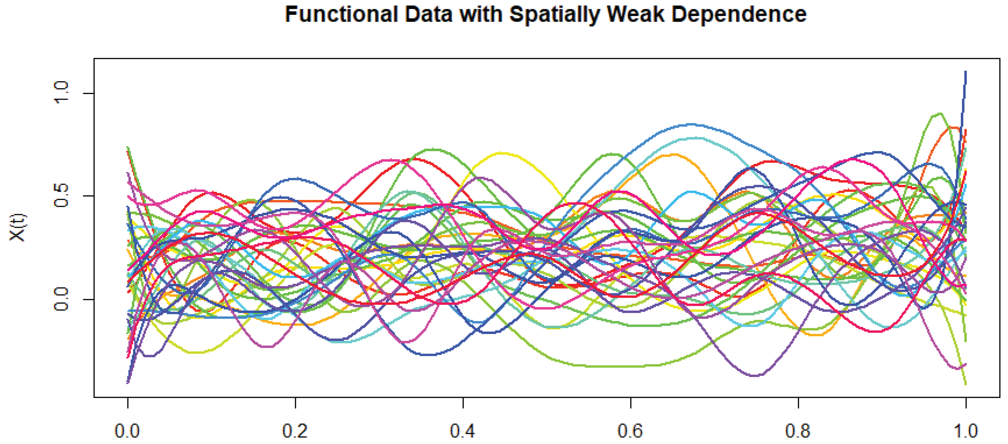
To illustrate the nature of the spatially weakly dependent functional covariates ${\mathcal{A}}_{\mathbf{i}}$, we plot a sample of these curves. Each function is observed on the interval $[0,1]$, and smoothness is ensured via B-spline basis functions.

As seen in Figure 1, we display a representative sample of 35 functional curves. These curves are smooth and exhibit gradual variability across space, consistent with the quasi-associated dependence structure. This visualization highlights the functional nature of the covariates and supports the assumptions used in our theoretical results.

4.3. Simulation Procedure

The simulation process proceeds as follows:

• Parameter Initialization: Define $n_1=n_2=10$, bandwidths $h_K$, $h_H$, and basis size (e.g., 15 B-splines). Choose functions $m\left(a\right)=\langle a,\psi \rangle$, and $\sigma \left(a\right)=0.3+0.1\parallel a\parallel$.
• Data Generation: Each functional covariate is generated as:

  $${\mathcal{A}}_{\mathbf{i}}\left(t\right)=\sum _{j=1}^J{\theta }_j^{\left(\mathbf{i}\right)}{\varphi }_j\left(t\right)+{\delta }_{\mathbf{i}}\left(t\right),$$

  where ${\theta }_j^{\left(\mathbf{i}\right)}\sim \mathcal{N}(0,0.3^2)$, and ${\delta }_{\mathbf{i}}$ is a spatially correlated perturbation modeled via exponential decay: $\mathrm{Cov}({\delta }_{\mathbf{i}},{\delta }_{\mathbf{j}})\propto exp(-\parallel \mathbf{i}-\mathbf{j}\parallel )$.
• Response Variable: For each $\mathbf{i}$, compute:

  $${\mathcal{B}}_{\mathbf{i}}=m\left({\mathcal{A}}_{\mathbf{i}}\right)+{\eta }_{\mathbf{i}},{\eta }_{\mathbf{i}}\sim \mathcal{N}(0,\sigma {\left(a\right)}^2).$$
• Kernel Estimation: We employ the nonparametric estimator defined in Equation (1), where $d(·,·)$ denotes the $L^2$ distance between functional covariates, H corresponds to the Gaussian cumulative distribution function, and K is the Epanechnikov kernel defined by:

  $$K\left(u\right)={\displaystyle \frac{3}{4}}(1-u^2){\mathbb{1}}_{\left\{\right|u|\le 1\}}.$$
  K is the Epanechnikov kernel, and H is the Gaussian CDF.
• Evaluation and Metrics: We compute pointwise metrics:

  $$\mathrm{Bias}(a,b)=\mathbb{E}\left[{\widehat{F}}_K(a,b)\right]-F^a\left(b\right),\mathrm{MSE}(a,b)=\mathbb{E}\left[{({\widehat{F}}_K(a,b)-F^a\left(b\right))}^2\right],$$

  estimated via Monte Carlo replications.
• Visualization: Plot ${\widehat{F}}_K(a,b)$ against $F^a\left(b\right)$ to visually assess the quality of the estimator across different ranges of b.

4.4. Results and Visual Analysis

To visually validate the performance of the kernel estimator, we plot the estimated conditional distribution function versus the true function for a fixed reference curve a. The figure below, generated from R, shows the estimated ${\widehat{F}}_K(a,b)$ in red (dashed) and the true function $F^a\left(b\right)$ in blue (solid).

Figure 2. Comparison between the estimated and true conditional distribution functions ${\widehat{F}}_K(a,b)$ and $F^a\left(b\right)$ for fixed functional input a.

Figure 2. Comparison between the estimated and true conditional distribution functions ${\widehat{F}}_K(a,b)$ and $F^a\left(b\right)$ for fixed functional input a.

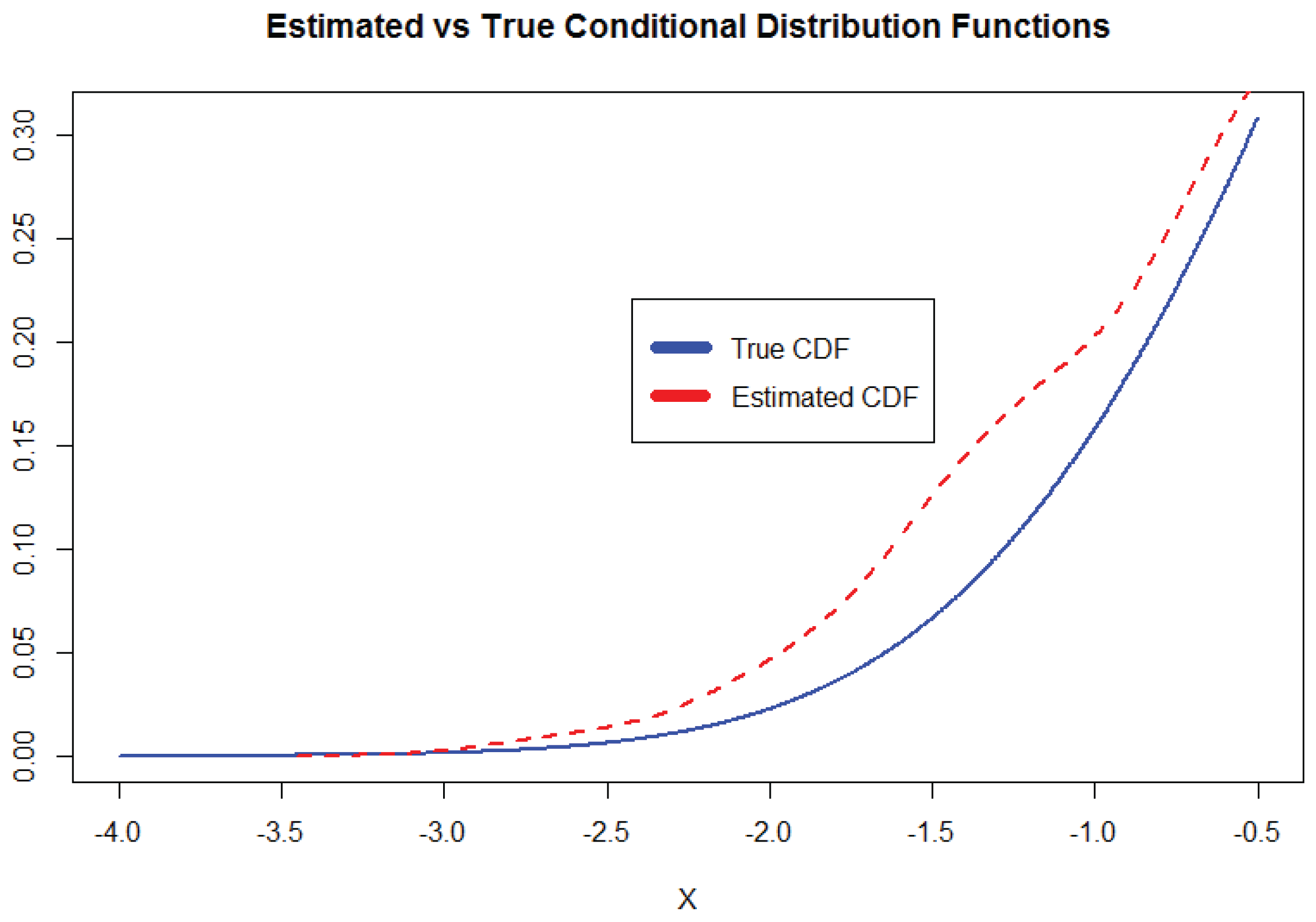
We observe that the estimator aligns closely with the true distribution in the central region. Slight overestimation near the tails may arise from finite-sample effects or boundary bias. Overall, the estimator exhibits robust behavior under weak spatial dependence and functional variability.

4.5. Summary of Findings

The kernel estimator performs well in capturing the true conditional distribution under spatially quasi-associated functional covariates. Simulation results corroborate the theoretical properties, particularly the convergence rate stated in Theorem 1. Estimation accuracy improves with increased sample size and suitable bandwidth selection. Visualization confirms strong agreement between estimated and true CDFs, with mild deviation at boundaries. This simulation study confirms the consistency and practical feasibility of the proposed estimator. It supports our asymptotic results and highlights its flexibility in the spatial functional context.

5. Conclusions and Perspectives

This study provides a comprehensive investigation of a kernel-type estimator for conditional distribution functions in the context of spatially indexed functional data, particularly when covariates take values in infinite-dimensional spaces. The core objective was to examine the asymptotic properties of the estimator, focusing on its almost complete convergence (a. co) and the associated convergence rates.

We considered a spatial sampling framework with quasi-associated dependence structures, reflecting realistic conditions in many applied settings. Under a set of regularity conditions, we derived uniform convergence results and provided theoretical guarantees for the performance of the estimator. The theoretical developments were supported by a simulation study, which confirmed the estimator’s consistency and highlighted its sensitivity to spatial correlation and bandwidth selection.

From a broader perspective, our findings emphasize the critical role of incorporating spatial structure into statistical modeling. Ignoring such dependence can lead to inaccurate inference, especially in high-dimensional or functional data settings. The kernel-based approach demonstrated here offers a flexible and nonparametric alternative, well-suited for complex spatial data.

Future Research Directions

Building upon this foundation, several promising avenues for further research emerge:

The current framework can be generalized to irregular spatial lattices or continuous spatial domains using tools from spatial stochastic processes.

Investigating the behavior of the estimator under deviations from the quasi-association assumption, heavy-tailed distributions, or outliers would enhance its practical relevance.

Developing adaptive or cross-validated procedures for selecting kernel bandwidths $h_K$ and $h_H$ remains an open challenge, especially in functional settings.

Applying the methodology to spatial datasets in geostatistics, climate science, or public health would provide practical insights and further validate the approach.

Creating efficient algorithms and open-source software for kernel estimation in spatially dependent functional data would facilitate broader adoption in applied contexts.

Overall, this work contributes to the understanding of nonparametric inference for conditional distributions in spatial data and lays the groundwork for future theoretical and applied developments in this growing area of statistical research.

References

- Newman, M. The Role of Research in This Association. Journal of School Health 1984, 54. [Google Scholar] [CrossRef]
- Aneiros, G.; Cao, R.; Fraiman, R.; Genest, C.; Vieu, P. Recent advances in functional data analysis and high-dimensional statistics. J. Multivariate Anal.170, 3–9. [CrossRef]
- Ramsay, J.; Silverman, B. W. Functional Data Analysis; Springer: New York, USA, 2005. [Google Scholar]
- Ramsay, J.; Hooker, G.; Graves, S. Functional Data Analysis with R and MATLAB; Springer: New York, USA, 2009. [Google Scholar]
- Doukhan, P.; Louhichi, S. A new weak dependence condition and applications to moment inequalities. Stochastic Process. Appl. 1999, 84, 313–342. [Google Scholar] [CrossRef]
- Matula, P. A note on the almost sure convergence of sums of negatively dependent random variables. Stat. Probab. Lett. 1992, 15, 209–213. [Google Scholar] [CrossRef]
- Newman, C.M. Asymptotic independence and limit theorems for positively and negatively dependent random variables. In Inequalities in Statistics and Probability; IMS Lecture Notes Monograph Series 1984, 5, 127–140. [Google Scholar]
- Roussas, G.G. Positive and negative dependence with some statistical applications. In Asymptotics, Nonparametrics and Time Series; Ghosh, S., Ed.; Marcel Dekker, Inc.: New York, USA, 1999; pp. 757–788. [Google Scholar]
- Doukhan, P.; Louhichi, S. A new weak dependence condition and applications to moment inequalities. Stochastic Process. Their Appl. 1999, 84, 313–342. [Google Scholar] [CrossRef]
- Bulinski, A.; Suquet, C. Normal approximation for quasi-associated random fields. Stat. Probab. Lett. 2001, 54, 215–226. [Google Scholar] [CrossRef]
- Douge, L. Théorèmes limites pour des variables quasi-associées hilbertiennes. Ann. Inst. Stat. Univ. Paris 2010, 54, 51–60. [Google Scholar]
- Attaoui, S.; Laksaci, A.; Ould-Said, E. Asymptotic Results for an M-estimator of the Regression Function for Quasi-Associated Processes. In Functional Statistics and Applications. Contributions to Statistics; Springer International Publishing: Cham, 2015; pp. 3–28. [Google Scholar] [CrossRef]
- Daoudi, H.; Mechab, B.; Chikr Elmezouar, Z. Asymptotic normality of a conditional hazard function estimate in the single index for quasi-associated data. Commun. Stat. Theory Methods 2020, 49, 513–530. [Google Scholar]
- Daoudi, H.; Mechab, B. Asymptotic Normality of the Kernel Estimate of Conditional Distribution Function for the quasi-associated data. Pak. J. Stat. Oper. Res. 2019, 15, 999–1015. [Google Scholar] [CrossRef]
- Daoudi, H.; Mechab, B.; Benaissa, S.; Rabhi, A. Asymptotic normality of the nonparametric conditional density function estimate with functional variables for the quasi-associated data. Int. J. Stat. Econ. 2019, 20, 94–106. [Google Scholar]
- Laksaci, A.; Mechab, W. Nonparametric relative regression for associated random variables. Metron 2016, 74, 75–97. [Google Scholar] [CrossRef]
- Allaoui, S.; Bouzebda, S.; Chesneau, C.; Liu, J. Uniform almost sure convergence and asymptotic distribution of the wavelet-based estimators of partial derivatives of multivariate density function under weak dependence. J. Nonparametr. Stat. 2021, 33, 170–196. [Google Scholar] [CrossRef]
- Bouaker, I.; Belguerna, A.; Daoudi, H. The consistency of the kernel estimation of the function conditional density for associated data in high-dimensional statistics. J. Sci. Arts 2022, 22, 247–256. [Google Scholar] [CrossRef]
- Daoudi, H.; Belguerna, A.; Elmezouar, Z.C.; Alshahrani, F. Conditional Density Kernel Estimation Under Random Censorship for Functional Weak Dependence Data. J. Math. 2025, Article ID 2159604. Available online: https://doi.org/10.1155/jom/2159604.
- Daoudi, H.; Elmezouar, Z.C.; Alshahrani, F. Asymptotic Results of Some Conditional Nonparametric Functional Parameters in High Dimensional Associated Data. Mathematics 2023, 11, 4290. [Google Scholar] [CrossRef]
- Bouzebda, S.; Laksaci, A.; Mohammedi, M. The k-nearest neighbors method in single index regression model for functional quasi-associated time series data. Rev. Mat. Complut. 2023, 36, 361–391. [Google Scholar] [CrossRef]
- Bouzebda, S.; Laksaci, A.; Mohammedi, M. Single Index Regression Model for Functional Quasi-Associated Time Series Data. REVSTAT-Statistical Journal 2023, 20, 605–631. [Google Scholar]
- Mechab, W.; Laksaci, A. Nonparametric relative regression for associated random variables. Metron 2016, 74, 75–97. [Google Scholar] [CrossRef]
- Daoudi, H.; Mechab, B.; Elmezouar, C.Z. Asymptotic Normality of a Conditional Hazard Function Estimate in the Single Index for Quasi-Associated Data. Commun. Stat. Theory Methods2018, Article ID 1549248.
- Tran, L.T. Kernel density estimation on random fields. J. Multivariate Anal. 1990, 34, 37–53. [Google Scholar] [CrossRef]
- Dabo-Niang, S.; Yao, A.F. Kernel regression estimation for continuous spatial processes. Math. Methods Statist. 2007, 16, 298–317. [Google Scholar] [CrossRef]
- Carbon, M.; Francq, C.; Tran, L.T. Kernel regression estimation for random fields. J. Statist. Plann. Inference 2007, 137, 778–798. [Google Scholar] [CrossRef]
- Li, J.; Tran, L.T. Nonparametric estimation of conditional expectation. J. Statist. Plann. Inference 2009, 139, 164–175. [Google Scholar] [CrossRef]
- Fix, E.; Hodges, J.L. Discriminatory Analysis, Nonparametric Discrimination: Consistency Properties. Technical Report 4, USAF School of Aviation Medicine, Randolph Field, 1951.
- Cover, T.M.; Hart, P.E. Nearest neighbor pattern classification. IEEE Trans. Inf. Theory 1967, 13, 21–27. [Google Scholar] [CrossRef]
- Cressie, N.A. Statistics for Spatial Data; Wiley: New York, USA, 1991. [Google Scholar]
- Biau, G.; Cadre, B. Nonparametric spatial prediction. Stat. Inference Stoch. Process. 2004, 7, 327–349. [Google Scholar] [CrossRef]
- Ferraty, F.; Rabhi, A.; Vieu, P. Estimation non-paramétrique de la fonction de hasard avec variable explicative fonctionnelle. Rev. Roumaine Math. Pures Appl. 2008, 53, 1–18. [Google Scholar]
- Masry, E. Recursive probability density estimation for weakly dependent stationary processes. IEEE Trans. Inf. Theory 1986, 32, 254–267. [Google Scholar] [CrossRef]
- Gasser, T.; Hall, P.; Presnell, B. Nonparametric estimation of the mode of a distribution of random curves. J. R. Stat. Soc. Ser. B 1998, 60, 681–691. [Google Scholar] [CrossRef]
- Ferraty, F.; Vieu, P. Nonparametric Functional Data Analysis: Theory and Practice; Springer Series in Statistics: New York, USA, 2006. [Google Scholar]
- Ferraty, F.; Laksaci, A.; Tadj, A.; Vieu, P. Rate of uniform consistency for nonparametric estimates with functional variables. J. Stat. Plann. Inference 2010, 140, 335–352. [Google Scholar] [CrossRef]
- Kara-Zaitri, L.; Laksaci, A.; Rachdi, M.; Vieu, P. Uniform in bandwidth consistency for various kernel estimators involving functional data. J. Nonparametr. Stat. 2017, 29, 85–107. [Google Scholar] [CrossRef]
- Ferraty, F.; Peuch, A.; Vieu, P. Modèle à indice fonctionnel simple. Comptes Rendus Math. 2003, 336, 1025–1028. [Google Scholar] [CrossRef]
- Ezzahrioui, M.; Ould-Saïd, E. Asymptotic Results of a Nonparametric Conditional Quantile Estimator for Functional Time Series. Commun. Stat. Theory Methods 2008, 37, 2735–2759. [Google Scholar] [CrossRef]
- Ezzahrioui, M.; Ould-Saïd, E. On the asymptotic properties of a nonparametric estimator of the conditional mode for functional dependent data. J. Nonparametr. Stat. 2008, 20, 3–18. [Google Scholar] [CrossRef]
- Laksaci, A. Convergence en moyenne quadratique de l’estimateur à noyau de la densité conditionnelle avec variable explicative fonctionnelle. Ann. Inst. Stat. Univ. Paris 2007, 51, 69–80. [Google Scholar]
- Laksaci, A.; Maref, F. Estimation non paramétrique de quantiles conditionnels pour des variables fonctionnelles spatialement dépendantes. Comptes Rendus Math. 2009, 347, 1075–1080. [Google Scholar] [CrossRef]
- Doob, J.L. Stochastic Processes; John Wiley and Sons: New York, USA, 1953. [Google Scholar]
- Kallabis, R.S.; Neumann, M.H. An exponential inequality under weak dependence. Bernoulli 2006, 12, 333–350. [Google Scholar] [CrossRef]
- Bosq, D. Linear Processes in Function Spaces: Theory and Applications; Lecture Notes in Statistics 149; Springer: Berlin/Heidelberg, Germany, 2000. [Google Scholar]
- Ramsay, J.O.; Silverman, B.W. Applied Functional Data Analysis: Methods and Case Studies; Springer-Verlag: New York, USA, 2002. [Google Scholar]
- Ferraty, F.; Laksaci, A.; Vieu, P. Estimating some characteristics of the conditional distribution in nonparametric functional models. Stat. Inference Stoch. Process. 2006, 9, 47–76. [Google Scholar] [CrossRef]
- Ferraty, F.; Laksaci, A.; Vieu, P. Functional time series prediction via conditional mode estimation. C. R. Math. Acad. Sci. Paris 2005, 340, 389–392. [Google Scholar] [CrossRef]
- Cardot, H.; Crambes, C.; Sarda, P. Spline estimation of conditional quantiles for functional covariates. C. R. Math. Acad. Sci. Paris 2004, 339, 141–144. [Google Scholar] [CrossRef]
- De Gooijer, J.; Gannoun, A. Nonparametric conditional predictive regions for time series. Comput. Statist. Data Anal. 2000, 33, 259–257. [Google Scholar] [CrossRef]
- Araujo, A.; Gin, E. The Central Limit Theorem for Real and Banach Valued Random Variables; Wiley Series in Probability and Mathematical Statistics; John Wiley and Sons: New York, NY, USA; Chichester, UK; Brisbane, Australia, 1980; p. xiv+233.
- Mohammedi, M.; Bouzebda, S.; Laksaci, A.; Bouanani, O. Asymptotic normality of the k-NN single index regression estimator for functional weak dependence data. Commun. Stat. Theory Methods 2022, 33, 1–26. [Google Scholar] [CrossRef]
- Daoudi, H.; Mechab, B.; Belguerna, A. Asymptotic Results of a Conditional Risk Function Estimate for Associated Data Case in High-Dimensional Statistics. In Proceedings of the International Conference on Recent Advances in Mathematics and Informatics (ICRAMI), 2021; Conference Paper. Available online: https://ieeexplore.ieee.org/document/9585904.
Figure 1.
Sample of 35 functional covariates , spatially quasi-associated.
Disclaimer/Publisher’s Note: The statements, opinions and data contained in all publications are solely those of the individual author(s) and contributor(s) and not of MDPI and/or the editor(s). MDPI and/or the editor(s) disclaim responsibility for any injury to people or property resulting from any ideas, methods, instructions or products referred to in the content. |
© 2025 by the authors. Licensee MDPI, Basel, Switzerland. This article is an open access article distributed under the terms and conditions of the Creative Commons Attribution (CC BY) license (http://creativecommons.org/licenses/by/4.0/).
Copyright: This open access article is published under a Creative Commons CC BY 4.0 license, which permit the free download, distribution, and reuse, provided that the author and preprint are cited in any reuse.