
Submitted:
25 August 2025
Posted:
26 August 2025
You are already at the latest version
Abstract
This paper investigates the asymptotic behavior of the conditional hazard function by kernel method , with particular focus on functional weakly dependent data. Specifically, we establish the asymptotic normality for the proposed estimator when the covariate be a functional quasi-associated process. This result contributes to the broader framework of nonparametric inference under weak dependence and functional data analysis. The estimator is constructed using kernel smoothing techniques inspired by the classical Nadaraya-Watson approach, and its theoretical properties are rigorously derived under suitable regularity conditions. To assess its practical performance, we carry out an extensive simulation study, comparing finite-sample results to their asymptotic counterparts. The findings demonstrate the robustness and reliability of the estimator across various settings, confirming the validity of the stated limit theorem in empirical contexts.
Keywords:
kernel method
; conditional hazard function
; almost consistency
; limit theorem
; quasi-associated functional data
MSC: 60E15; 60G50; 62J02; 62M10
1. Introduction
Recent advances in computational technology and data acquisition systems have made it possible to store and process massive datasets that vary over time, including curves and images. These types of observations are commonly referred to as functional data. Effectively analyzing and modeling such data presents both a challenge and an opportunity for statisticians, leading to the development of powerful statistical tools—chief among them, nonparametric estimation methods.
Pioneering contributions by Bosq and Lecoutre [1], Ferraty and Vieu [2], Ferraty, Mas, and Vieu [3], and Laksaci and Mechab [4] have laid the foundation for nonparametric estimation in the functional data context. Their works have significantly influenced the theoretical aspect and practical implementation of kernel method, making them key references in the domain of nonparametric functional statistics.
Numerous researchers have addressed the study of nonparametric models from both theoretical and practical perspectives. For instance, in the context of kernel estimation, Ferraty and Vieu [5], and Ferraty, Goia, and Vieu [6] investigated regression operators for functional data. Laksaci and Mechab [7] explored the asymptotic behavior of regression functions under weak dependence, Azzi et al. [8] present the function modal regression for functional data, while Hyndman and Yao [9] proposed estimation techniques and symmetry tests for conditional density functions. Daoudi et al. [10] show conditional density estimation under weak dependence and Censorship phenomena. Other notable contributions include those of Attaoui, Laksaci, and Ould Said [11], as well as Xu [12] and Abdelhak et al. [13], who studied single-index models, Daoudi and Mechab [14], who focused on estimating the conditional distribution function under quasi-association assumptions.
These contributions, centered around kernel-based methods for conditional models, have led to significant insights into the asymptotic properties of estimators related to prediction, conditional distribution functions, and their derivatives, particularly the conditional density function. Furthermore, Bulinski and Suquet [15] examined random fields with both positive and negative dependence structures, Bouaker et al. [16] examine the consistency of the kernel estimator for conditional density in high dimensional statistics, and Newman [17] investigated asymptotic independence and limit theorems in similar settings.
Regarding the hazard function, several works have addressed its estimation in dependent contexts. Ferraty, Rabhi, and Vieu [18], Laksaci and Mechab [19], and Gagui and Chouaf [20] obtained the asymptotic normality results in the case of -mixing conditions. Belguerna et al. [21] further analyzed the MSE of the conditional hazard function estimator.
The concept of quasi-association for real-valued stochastic processes, presented in [22] as a particular form of weak dependence, was later extended by Bulinski and Suquet [23]. Further contributions were made by Kallabis and Neumann [24], who derived exponential inequalities under weak dependence conditions.
More recently, a number of studies have investigated nonparametric models involving quasi-associated random variables. Bassoudi et al. [25] evaluate the asymptotic characteristics of the conditional hazard estimator derived from the local linear technique for ergodic data. Attaoui [26], Tabti and Ait Saidi [27], and Douge [28] have contributed to this direction.
Furthermore, recent research has increasingly focused on the asymptotic analysis of conditional functional models under weak dependence structures, particularly quasi-association. Daoudi, Mechab, and Chikr Elmezouar [29], as well as Daoudi et al. [30], have investigated asymptotic properties of estimators of conditional hazard functions in single-index models for quasi-associated data. Similarly, Bouzebda, Laksaci, and Mohammedi [31] studied the single-index regression model, while Rassoul et al. [32] examined the mean squared error of the conditional hazard rate, highlighting its asymptotic behavior under weak dependence assumptions. Daoudi et al. [35] demonstrate asymptotic results of a conditional risk function estimate for associated data case in high-dimensional statistics.
In the same context, additional contributions have strengthened the theoretical foundation of kernel-based nonparametric estimators. For instance, the asymptotic normality and consistency of the conditional density and hazard function estimators have been addressed under quasi-associated and weakly dependent functional data settings [33]. High-dimensional statistics and complex dependence frameworks have also been tackled, including the asymptotic behavior of regression estimator under quasi-associated functional censored time series [35] and [36]. These works confirm the growing interest in developing robust asymptotic results for conditional models in dependent functional data, offering theoretical tools that support their practical implementation.
This study examines the asymptotic characteristics of the conditional hazard function estimator for functional data under quasi-associated phenomena, with the aim of establishing its asymptotic properties. We begin by introducing the functional model along with all necessary notation and mathematical tools. As a first result, we establish the almost complete consistency. Then, we derive its asymptotic normality by employing various analytical techniques and decomposition strategies. All theoretical developments are supported with rigorous proofs.
To validate the theoretical findings, we conduct a numerical study demonstrating the asymptotic normal approximation of the proposed estimator. In this context, we generate three datasets of different sizes to examine the impact of key parameters such as sample size and bandwidth on estimator performance. Graphical comparisons between theoretical and empirical results are provided to illustrate the estimator’s effectiveness and assess the quality of the estimation.
This paper is structured as follows. In Section 2, we present the quasi-associated sequence, outline the model construction, and present the estimator. Section 3 states the necessary assumptions and develops the results concerning almost complete convergence and asymptotic normality of the estimator. Section 4 provides a comprehensive numerical study supporting the theoretical findings and offering asymptotic confidence bounds. Finally, the detailed proofs of our main results are given in Appendices Appendix A and Appendix B.
2. The Model
Let , be an -valued measurable and strictly stationary stochastic process defined on a probability space , where denotes a semi metric space, where is a normed Hilbert space, provided with an inner product . The semi metric noted d defined by . We consider a fixed point s in , a fixed neighborhood of s and be a fixed compact subset of . We assume the existence of a regular version of the conditional probability distribution of the random variable T given S. Furthermore, for all , we suppose that the conditional distribution function of T given denoted by is three times continuously differentiable. We denote its corresponding conditional density function by .
In this paper, we investigate the kernel estimation of the conditional hazard function of T given , denoted , for all such that , is given by:
In our functional context, the kernel estimate of this function is given by:
where is the conditional distribution functional estimator, given by:
and is the conditional density functional estimator, given by:
with K denote a kernel function, H be a given differentiable distribution function with derivative . The quantities and represent sequences of positive bandwidth parameters. Under this framework, the estimator can be expressed as:
where
with notational convenience:
Our primary objective is to establish both the consistency and the asymptotic normality of the estimator (4) under suitable hypothesis, where the sequence of variables verify the quasi-association as defined by Bulinski and Suquet [18].
Definition 1.
Given and subsets of where , for all lipschitzian and functions, we consider as a sequence of quasi associated random vector if :
represent the component of , defined as , where is an orthonormal basis.
3. Main Results
3.1. Assumptions
In the sequel, when no confusion will likely to arise, we will denote by and strictly positive constants, and by the covariance coefficient defined as:
Where
For , let be a small ball, shis center and his radius.
To achieve the desired goal, we begin by stating the following required assumptions.
- ()
- , and is a differentiable at 0. Moreover, such that
- ()
- Assume that the Hölder continuity condition is hold for both functions and .for all and , with constants , , and be a subset of ( compact).
- ()
- H is an even and bounded function, with a bounded and Lipschitz continuous derivative , satisfying:
- ()
-
For a differentiable, Lipschitz continuous and bounded kernel K, and such:: is the indicator function on , is derivative of with:.
- ()
- The random pairs is a quasi-associated sequence with covariance coefficient , satisfying :
- ()
- ()
-
The bandwidths and satisfy :
- i-
- ,
- ii-
- and .
- iii-
- ()
-
For , the functions andare derivable at 0.
3.2. Comments on the Assumptions
() This assumption specifies conditions governing the probability that S lies within a neighborhood of s, along with the consistence behavior of the corresponding probability ratio as the neighborhood size approaches zero. These conditions are essential for applying local convergence theorems. () The Hölder continuity assumption imposed on the conditional distribution and their derivatives represents a standard regularity condition in the literature. (), (), and () are technical, ensuring the convergence of the convolution kernel, and enabling the use of Taylor expansions. () This quasi-association assumption on the data is interesting, as it covers a more general framework than classical independence. () This assumption characterizes the asymptotic behavior of the joint distribution. () This last assumption concerns the control of the joint probability of two S variables in a neighborhood of s, which helps control the covariance terms in the asymptotic developments. Such assumptions are typical in the setting of nonparametric estimation when dealing with functional covariate.
3.3. Main Results
3.3.1. The Almost Consistency
Our goal is to derive the almost complete convergence (a.co.) of to , and this result is formalized in the following theorem.
Theorem 1.
Under the conditions ()-(), we have
Proof
(Proof of theorem 1). needed this decomposition:
And the following subsequent results.
Lemma 1.Under the assumptions (), ()-(), and for any fixed t, we have
Lemma 2.Assuming that the conditions ()-() hold, then for , we infer:
where
Corollary 1. Making use the assumptions ()-(), we get:
Lemma 3. Under the assumptions of Theorem 1
And
with
□
3.3.2. Asymptotic Normality
Theorem 2.
Under ()-(), we infer:
where
and is defined in Lemma 3.
Proof of Theorem 2.
Needed the decomposition (6), the results shown in above Lemmas (2 and 3) and the following subsequent result (Lemma 4):
Lemma 4. Assuming that ()-() hold, then
with
The rigorous proof and demonstrations of the intermediate results (Lemmas 1,2,3 and 4), and Corollary □
4. Application and Numerical Study
4.1. Confidence Bounds
Constructing reliable confidence bounds is a key aspect of statistical analysis, as they characterize the variability and reliability of model estimators. Proper interpretation of these bounds enables more informed and robust conclusions about the underlying estimator. In the context of survival and hazard function estimation, confidence bounds are particularly valuable since they provide a quantitative assessment of the uncertainty surrounding the estimated conditional hazard function, thereby guiding both theoretical analysis and practical decision-making. Moreover, confidence bounds serve as a diagnostic tool: narrow bounds suggest stable and precise estimators, while wider bounds highlight regions where the estimator is less reliable due to limited data or high variability.
As an application of the result established in Theorem 2, we construct confidence bounds for at the confidence level . To this end, we must first estimate the unknown components of the asymptotic variance as follows: these include the conditional density, the conditional survival function, and kernel-based quantities that appear in the variance expression. Consistent estimation of these components is essential, since any bias or misspecification would directly affect the coverage probability of the resulting bounds. Once these quantities are estimated, the asymptotic normality result in Theorem 2 allows us to approximate the distribution of the estimator and derive pointwise confidence intervals for across the range of t. This methodology not only validates the theoretical properties of the proposed estimator but also ensures its applicability in empirical studies where inference on the conditional hazard function is required.
where represents the cardinality of the set A. Also, is estimated by:
Corollary 2.
When the assumptions of Theorem 2 hold, we set:
Moreover, the confidence bounds will be,
where is the quartile of .
4.2. Numerical Study
In this part, we conduct a numerical study using R software to illustrate and validate the theoretical results through graphical representations. The aim of this simulation is to assess the finite-sample performance of the proposed estimator and to highlight the extent to which the asymptotic properties established in the theoretical framework are reflected in practice. By generating controlled data under specific dependence structures and censoring mechanisms, we are able to visualize the behavior of the conditional density and hazard estimators, compare them with their theoretical counterparts, and evaluate their accuracy across different sample sizes. This numerical experiment also provides insights into the rate of convergence, the influence of the smoothing parameters, and the robustness of the estimator under varying conditions.
This simulation is based on the following points: we describe the data-generating process and the dependence structure imposed, specify the choice of kernel functions and bandwidths, outline the implementation of the random censoring mechanism, and finally present the graphical outputs and error metrics that allow for a systematic comparison between theoretical and empirical curves. The numerical results obtained will not only complement the theoretical findings but also serve as practical evidence of the efficiency and reliability of the proposed estimation methodology.
-
Definite our model by choosing functional covariate as :The process satisfies a specific dependence structure,namely a quasi-associated sequence, which is generated as a non-strong mixing auto-regressive process of order 1. This process is constructed by setting the auto-regressive coefficient and modeling the innovation term as a binomial distribution [18]. We use 100 discretization points of u to obtain the curves shown below in Figure 1, Figure 2 and Figure 3, corresponding to different sample sizes.For the real variable is defined as . Where m is the nonlinear regression operator,Where is standard normal distribution. Its clear that the explicit form of the conditional density given by:. In the next, we select the distance in as:Also.
-
A bandwidth Selection Algorithm: The smoothness of the estimators (2) and (3) is controlled by the smoothing parameter and the regularity of the cumulative distribution function (CDF). Therefore, choosing these parameters plays a critical role in the computational process. An optimal selection leads to effective estimation with a small mean squared error (MSE), which, for the conditional hazard function, is given by:Let be a distribution function on and . Note that as .This indicates that can be interpreted as a regression of on , Consequently, we adapt this regression framework to our estimation problem. By combining this approach with the normal reference rule [7], we derive an effective algorithm for selecting the bandwidth parameters.
- i-
- Compute the bandwidth using the normal reference rule.
- ii-
- Given , use cross-validation (as proposed by [1]) to determine the optimal value of (using the function fregre.np.cv in the package fda.usc) for our calculation of .
-
Calculate the estimates of both the conditional distribution and the conditional density functions, and compare these estimates with their theoretical counterparts on the same graphs.(Figure 4 and Figure 5).It is apparent that our estimations exhibit high accuracy when optimal bandwidths are selected. To assess the performance of each model more rigorously, we compute the mean squared error, as shown in Table 1.For the next step in achieving the desired objective and firmly establishing the normal approximation of with high effectiveness, we selected the sample that produced an estimate with the smallest MSE (sample size ), and followed the subsequent steps:
5. Conclusion and Some Perspectives
Due to the complexity of the conditional hazard function estimate by the kernel approach, we began by decomposing the estimator into three parts, as shown in (6). The first part corresponds to the numerator of the density function estimator, denoted , which is considered the dominant component influencing the estimator’s properties. We showed that the denominator of the corresponding term converges in probability to . The remaining two parts account for the bias in both the conditional distribution and density function estimators, arising from and .
From a practical perspective, we conducted a simulation study to validate the theoretical findings. Despite the inherent challenges in selecting and tuning parameters such as bandwidths, the proposed estimator demonstrated strong performance, achieving a low mean squared error.
These results are promising and contribute to the growing body of research in this field. However, further investigation is needed to assess the robustness of the method in diverse real-world settings and to explore potential extensions that could improve its applicability and generalizability.
A potential direction for future work is to examine the sensitivity of the estimator to kernel choice and bandwidth selection procedures. Exploring data-driven or adaptive bandwidth strategies may enhance finite-sample performance. Additionally, investigating the behavior of the estimator in high-dimensional or complex data settings could broaden its practical utility.
This study enhances both the theoretical and empirical comprehension of the asymptotic characteristics of the proposed estimator, laying the foundation for future developments and applications in areas where estimating conditional functional parameters is essential.
Author Contributions
Conceptualization, A.R., Z.C.E., H.D. and A.B.; methodology, Z.C.E. and H.D.; software, A.R.; validation, Z.C.E., A.B., and H.D.; formal analysis, A.R., Z.C.E., F.A. and H.D.; investigation, A.R., Z.C.E., F.A., A.B., and H.D.; resources, A.R., Z.C.E., F.A. and H.D.; data curation, A.R.; writing original draft preparation, H.D. and A.R.; writing review and editing, A.R.,Z.C.E., A.B, and H.D.; visualization, A.R. and H.D.; supervision, Z.C.E. and F.A.; project administration, Z.C.E.; funding acquisition, Z.C.E. and F.A. All authors have read and approved the final version of the manuscript for publication.
Funding
This research project was funded by (1) Princess Nourah bint Abdulrahman University Researchers Supporting Project Number (PNURSP2023R358), Princess Nourah bint Abdulrahman University, Riyadh, Saudi Arabia, and (2) The Deanship of Research and Graduate Studies at King Khaled University for funding this work through small under grant numbergroup research RGP1/163/45
Data Availability Statement
The data used to support the findings of this study are available on request from the corresponding author.
Acknowledgments
The authors thank and express their sincere appreciation to the funders of this work: (1) Princess Nourah bint Abdulrahman University Researchers Supporting Project (Project Number: PNURSP2025R358), Princess Nourah bint Abdulrahman University, Riyadh, Saudi Arabia; (2) The Deanship of Scientific Research at King Khalid University, through the Research Groups Program under grant number R.G.P. 1/118/46.
Conflicts of Interest
The authors declare no conflict of interest.
Appendix A
Proof of Lemma 1.
The proof of this lemma is based on the exponential inequality of Kallabis and Nymann which is given in the following lemma:
Lemma A1. [19] Let real random variables with and for all and , let .
Assume that there exist and such that the following inequality is true for all u-tuplets and r-tuplets with
Then,
for some
We use Lemma 1 on the variables:
Where moreover, we have:
And
In order to apply Lemma 1 we have to choose the variable which is conditioned by the variance of , starting by upper bound the as follow:
Where,
Thus, under () and (), and by integration on the real component z It follows that
We show for n enough large using Taylor expansion (first order)
Hence
We denote by for , then
In accordance with Ferraty et al.[2] (refer to Lemma 1, page 26), we establish:
The last line is justified by the order of the Taylor expansion for around 0, and . Additionally, we employ the results of Lemma 2 on page 27 in Ferraty et al.[2].
Then, (A4) become,
This enables us to deduce
For the 2nd term in the equation(A3), by the same steps followed above, () satisfy, we demonstrate
Which implies that
And
For the 2nd term , we decompose the sum in 2 sets by with , as .
Under assumptions (), () and (), we infer for
Now, under the assumptions ()-(), we set
Taking , we get
Now, we need to evaluate the the covariance term , for all and with . For that we distingue the following cases:
The variables fulfill the requirements of Lemma 1 for:
Thus,
Where
Hence
Finally, for a suitable choice of , the proof is achieved. □
Proof
(Proof of Lemma 2). Taking , using the stationarity property, we can write:
-
For the bias term ofWithUsing a Taylor expansion of the function :Under (A21) and hypothesis (), we deduce:Denote by for , thenWhereWith the same steps following to evaluate (A5), we set:The last line justifies by the order Taylor expansion for around 0. Additionally, we employ the results of Ferraty et al.[2] (Lemma 2, page 27).Which allow us under (A25) to set:Hence,
-
For the bias term of , we start by writing:Using a Taylor expansion under (), we infer:The same steps used to studying can be followed ( see Rassoul et al. [36] page 16) to infer that:
□
Proof of Corollary 1.
Using (A1), we can write:
Then, to calculate , we replace by and follow the same steps used in the evaluation of (A2), in conclusion, we get:
For the second result about , keeping the same notation with respect the definition of in (5), we set
Moreover,
Furthermore, the 2nd term , we decompose as follows:
Now, under the assumption (), we have
From the condition (), we infer that
This implies that
Next, taking
which allows to write that:
Finally, we get:
Now we evaluate as follows:
Where
For the first term in right-hand of (A31), we have
The first order Taylor expansion of G around t for n large enough justified the last line, furthermore, replacing K by in (A24), and following the same steps and techniques, then by the fact that , the second term allow us to get:
Then,
Furthermore, for the 2nd term , we follow the steps used to analysis in lemma 1, we divide the sum below:
We keep the same notation and under hypothesis (), () and (), we infer,
Both K and H are bounded, so :
Taking , we get:
□
Proof of Lemma 3.
It is clear that the result of Lemma 2 and corollary 1 permits to write:
And
Then, by Markov Inequality:
Finally, by combining this result with the fact that
we get the required result. □
Appendix B
Proof
(Proof of Lemma 3). By the definition of in (5), it follows that
Where
And
The result is:
To do this, we employ Doob’s basic technique ( pages 228-231)[26]. We indeed choose two sequences of natural numbers that extend to infinity.
And we divide into
Where
With
Remark that, for , , we have , and , which means as as . Our asymptotic result is now founded on:
and
Proof of (A41). Stationary gives us:
And
Using (A10) and the fact that . we set
In the other side, we have
Similarly to (A11), we write for this last covariance;
Thus, by the same steps using to evaluate (A11) we obtain:
Then
For the second term of (A43), we use the stationary to evaluate the right-hand side.
For all , we have , then
By this last result and (A49) we set:
By the fact we get for the sequence ;
Hence,
Proof of (A42). based in the following two results
And
□
roof of (A52).
And successively, we have:
Once again we apply Lemma 1, to write:
For all , we have then
Therefore, inequality (A54) becomes
□
Proof of (A53). By the definition of and , we have
Using the result of (A9) and the fact that , Which imply that
For the second term of (A53), we conclude by , and Tchebychev’s inequality to get:
This concludes Lemma 3’s proof. □
References
- D. Bosq, J.B. Lecoutre, Théorie de l’estimation fonctionnelle, Ed. Economica, (1987).
- F. Ferraty, P. Vieu, Nonparametric functional data analysis: Theory and practice, Springer Series in Statistics, Springer, Berlin (2006) ISBN 978-0-387-30369-7.
- F. Ferraty, A. Mas, And P. Vieu, Nonparametric regression on functional data: inference and practical aspects, Australian and New Zealand Journal of Statistics, 49 (2007), 267–286. [CrossRef]
- A. Lakcasi, B. Mechab, Conditional hazard estimate for functional random fields., Journal of Statistical Theory and Practice, 08 (2014), 192-220. [CrossRef]
- F. Ferraty, P. Vieu, Nonparametric models for functional data, with application in regression, time series prediction and curve discrimination, Journal of Nonparametric Statistics, 16 (2004), 111–125. [CrossRef]
- F. Ferraty, A. Goia, P. Vieu, Régression non-paramétrique pour des variables aléatoires fonctionnelles mélangeantes, Comptes Rendus Mathematique, 334 (2002), 217-220. [CrossRef]
- W. Mechab, A. Lakcasi, Nonparametric relative regression for associated random variables, Metron, 74 (2016), 75-97. [CrossRef]
- Azzi, A., Belguerna, A., Laksaci, A., & Rachdi, M. (2023). The scalar-on-function modal regression for functional time series data. Journal of Nonparametric Statistics, 36(2), 503–526. [CrossRef]
- R.J. Hyndman, Q. Yao, Nonparametric estimation and symmetry tests for conditional density functions, Journal of Nonparametric Statistics, 14 (2002), 259–278. [CrossRef]
- H. Daoudi, A. Belguerna, Z. C. Elmezouar, F. Alshahrani, Conditional Density Kernel Estimation Under Random Censorship for Functional Weak Dependence Data. Journal of mathematics. 2159604 (2025). [CrossRef]
- S. Attaoui, A. Laksaci, E. Ould Said, A note on the conditional density estimate in the single functional index model, Statistics and Probability Letters, 81 (2011), 45–53. [CrossRef]
- N. Ling, Q. Xu, Asymptotic normality of conditional density estimation in the single index model for functional time series data, Statistics and Probability Letters, 82 (2012), 2235-2243. [CrossRef]
- K. Abdelhak, A. Belguerna, and Z Laala, Local Linear Estimator of the Conditional Hazard Function for Index Model in Case of Missing at Random Data, Applications and Applied Mathematics: An International Journal (AAM), 17(1), (2022). https://digitalcommons.pvamu.
- H. Daoudi, B. Mechab, Asymptotic Normality of the Kernel Estimate of Conditional Distribution Function for the quasi-associated data, Pakistan Journal of Statistics and Operation Research, 15 (2019), 999–1015. [CrossRef]
- A. Bulinski, C. Suquet, Asymptotical behaviour of some functionals of positively and negatively dependent random fields, Fundamentalnaya i Prikladnaya Matematika, 04 (1998), 479-492. https://www.mathnet.
- I. Bouaker, A. Belguerna, H. Daoudi, The Consistency of the Kernel Estimation of the Function Conditional Density for Quasi-Associated Data in High-Dimensional Statistics, Journal of Science and Arts, 22 (2022), 247–256. [CrossRef]
- C.M. Newman, Asymptotic independence and limit theorems for positively and negatively dependent random variables : Inequalities in Statistics and Probability, Lecture Notes-Monograph Series, 05 (1984), 127-140. http://www.jstor.org/stable/4355492.
- F. Ferraty, A. Rabhi And F. Vieu, Estimation nonparametric de la fonction de hasard avec variable explicative fonctionnelle, Revue roumaine de mathématiques pures et appliquées, 53 (2008), 1-18.
- A. Laksaci, B. Mechab, Estimation non-paramétrique de la fonctionde hasard avec variable explicative fonctionnelle : cas des données spatiales, Revue roumaine de mathématiques pures et appliquées, 55 (2010), 35–51.
- A. Gagui, A. Chouaf, On the nonparametric estimation of the conditional hazard estimator in a single functional index, Statistics in Transition new series, 23 (2022), 89–105. [CrossRef]
- A. Belguerna, H. Daoudi, K. Abdelhak, B. Mechab, Z. Chikr Elmezouar, F. Alshahrani, A Comprehensive Analysis of MSE in Estimating Conditional Hazard Functions: A Local Linear, Single Index Approach for MAR Scenarios, Mathematics, 12 (2024), 495. [CrossRef]
- P. Doukhan, S. Louhichi, A new weak dependence condition and applications to moment inequalities, Stochastic Processes and their Applications, 84 (1999), 313–342. [CrossRef]
- A. Bulinski, C. Suquet, approximation for quasi-associated random fields., Statistics and Probability Letters, 54 (2001), 215–226. [CrossRef]
- R.S. Kallabis, M.H. Neumann, An exponential inequality under weak dependence, Bernoulli, 12 (2006), 333–350.
- M. Bassoudi, A. Belguerna, H. Daoudi And Z. Laala, Asymptotic properties of the conditional hazard function estimate by the local linear method for functional ergodic data, journal of Applied Mathematics and Informatics, 41 (2023), 1341-364. [CrossRef]
- S. Attaoui, Sur l’estimation semi paramètrique robuste pour statistique fonctionnelle, Université du Littoral Côte d’Opale Sciences pour l’Ingénieur (Lille); Université Djillali Liabès (Sidi Bel-Abbès, Algérie), (2012).
- H. Tabti, A. Ait Saidi, Estimation and simulation of conditional hazard function in the quasi-associated framework when the observations are linked via a functional single-index structure, Communications in Statistics - Theory and Methods, 47 (2017), 816-–838. [CrossRef]
- L. Douge, Thèorèmes limites pour des variables quasi-associes hilbertiennes, annales de l’ISUP, 04 (2010), 51–60.
- H. Daoudi, B. Mechab, Z. Chikr Elmezouar, Asymptotic normality of a conditional hazard function estimate in the single index for quasi-associated data, Communications in Statistics - Theory and Methods, 49 (2020), 513–530. [CrossRef]
- H. Daoudi, Z. Chikr Elmezouar, F. Alshahrani, Asymptotic Results of Some Conditional Nonparametric Functional Parameters in High Dimensional Associated Data, Mathematics, 11 (2023), 4290. [CrossRef]
- S. Bouzebda, A. Laksaci, M. Mohammedi, Single Index Regression Model for Functional Quasi-Associated Times Series Data, REVSTAT-Statistical Journal, 20 (2023), 605–631. [CrossRef]
- A. Rassoul, A. Belguerna, H. Daoudi, Z. C. Elmezouar, F. Alshahrani, On the Exact Asymptotic Error of the Kernel Estimator of the Conditional Hazard Function for Quasi-Associated Functional Variables, mathematics, 13(13) (2025).
- H. Daoudi, B. Mechab, S. Benaissa, A. Rabhi, Asymptotic normality of the nonparametric conditional density function estimate with functional variables for the quasi-associated data. Int. J. Stat. Econ. 20 (2019). http://www.ceser.in/ceserp/index.php/bse/article/view/6131.
- H. Daoudi, B. Mechab and A. Belguerna, Asymptotic Results of a Conditional Risk Function Estimate for Associated Data Case in High-Dimensional Statistics, Asymptotic Results of a Conditional Risk Function Estimate for Associated Data Case in High-Dimensional Statistics, Tebessa, Algeria, 2021, pp. 1-6. [CrossRef]
- S. Attaoui, O. Benouda, S. Bouzebda, A. Laksaci, Limit theorems for kernel regression estimator for quasi-associated functional censored time series within single index structure, Mathematics, 13 (2025). [CrossRef]
- J. L. Doob, Stochastic Processes, Wiley, New York (1953), pp. 228-231.
Figure 1.
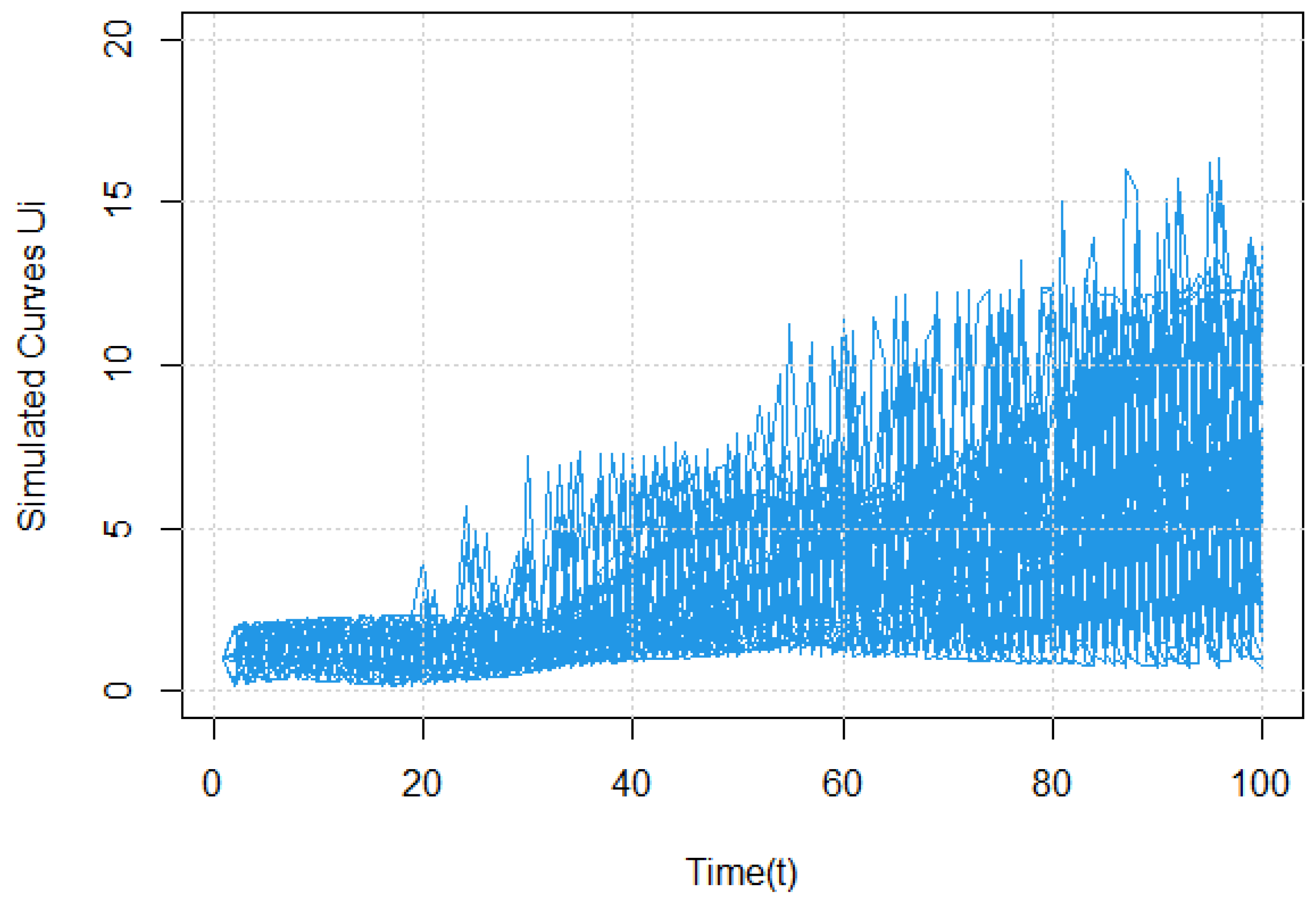
Figure 2.
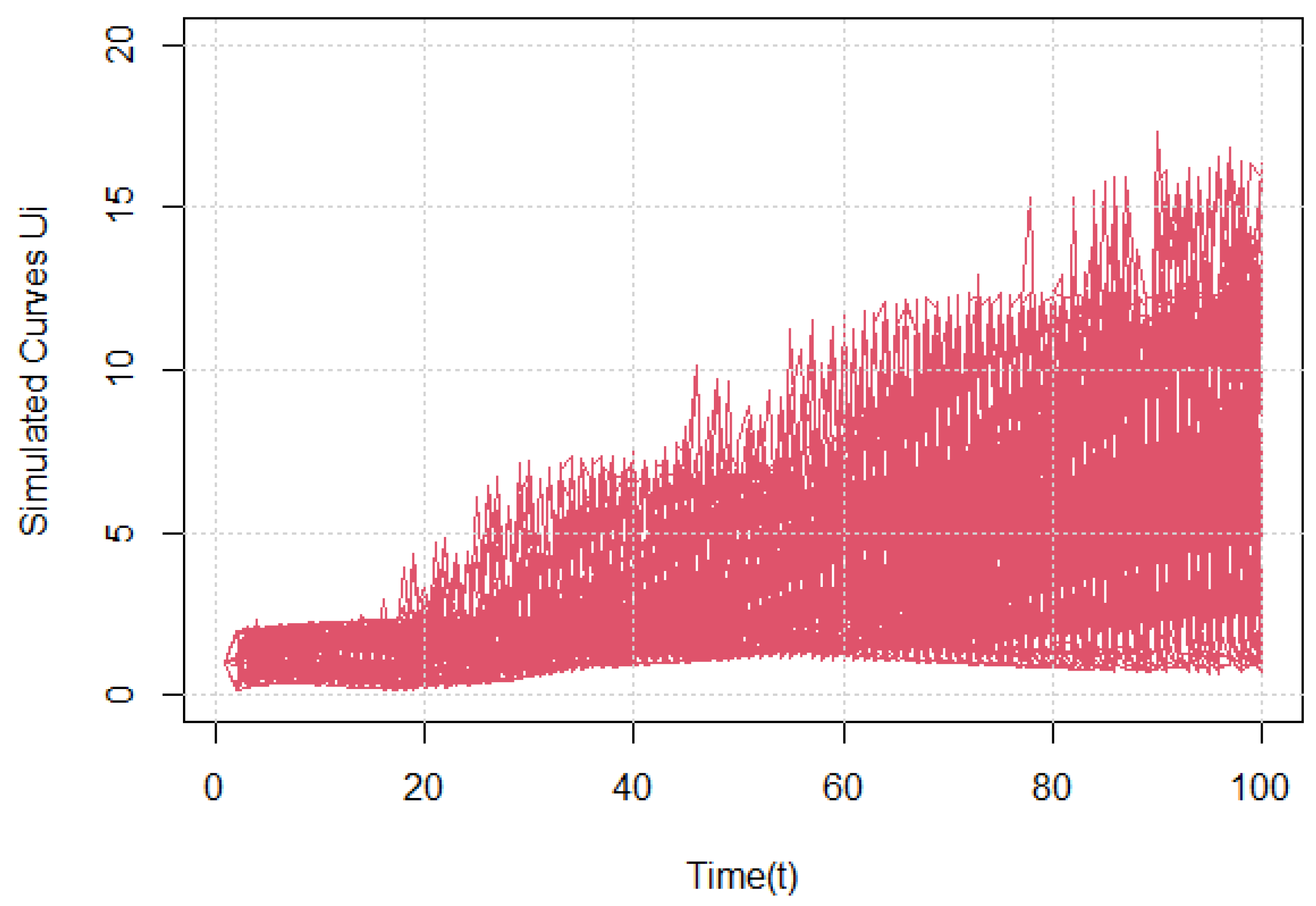
Figure 3.
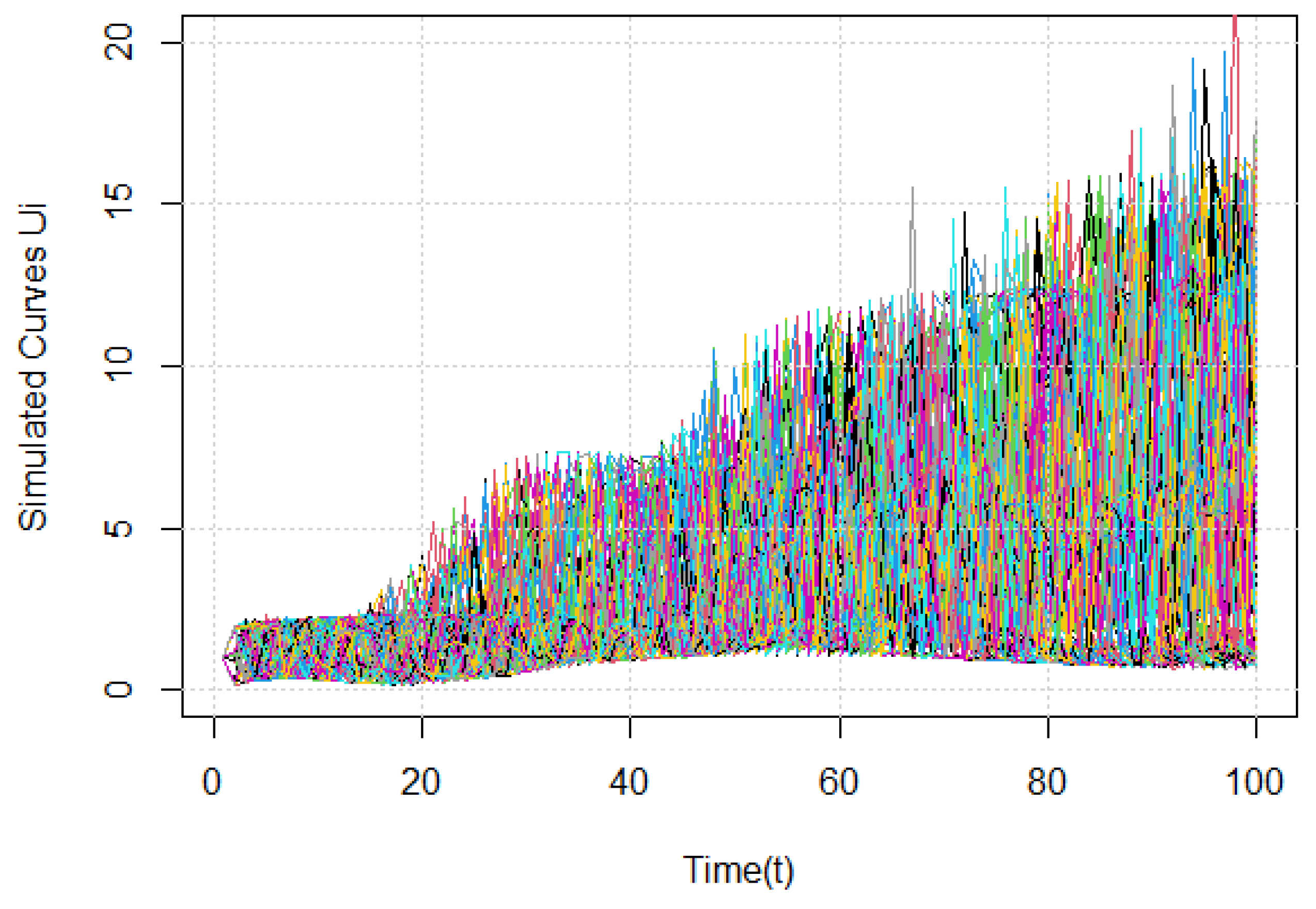
Figure 4.
Conditional distribution
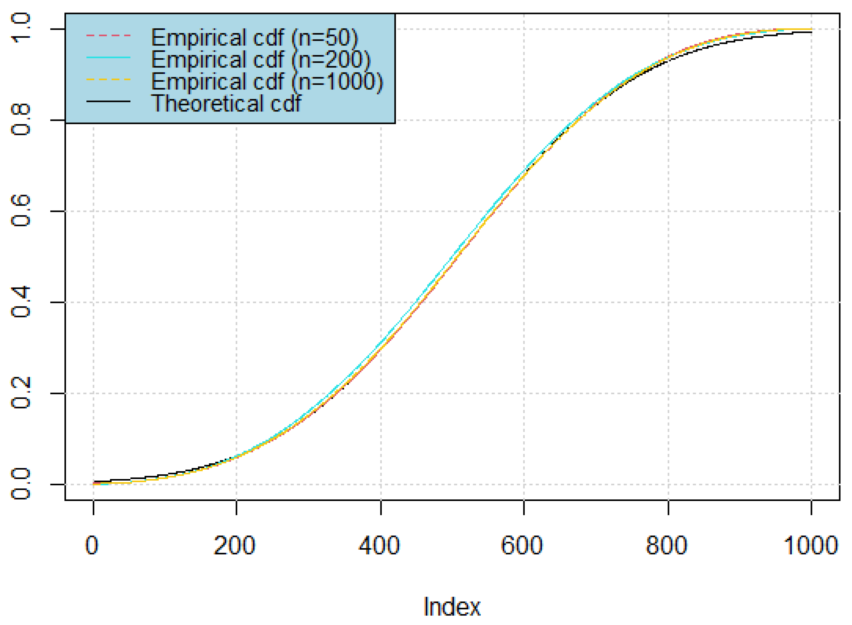
Figure 5.
Conditional density
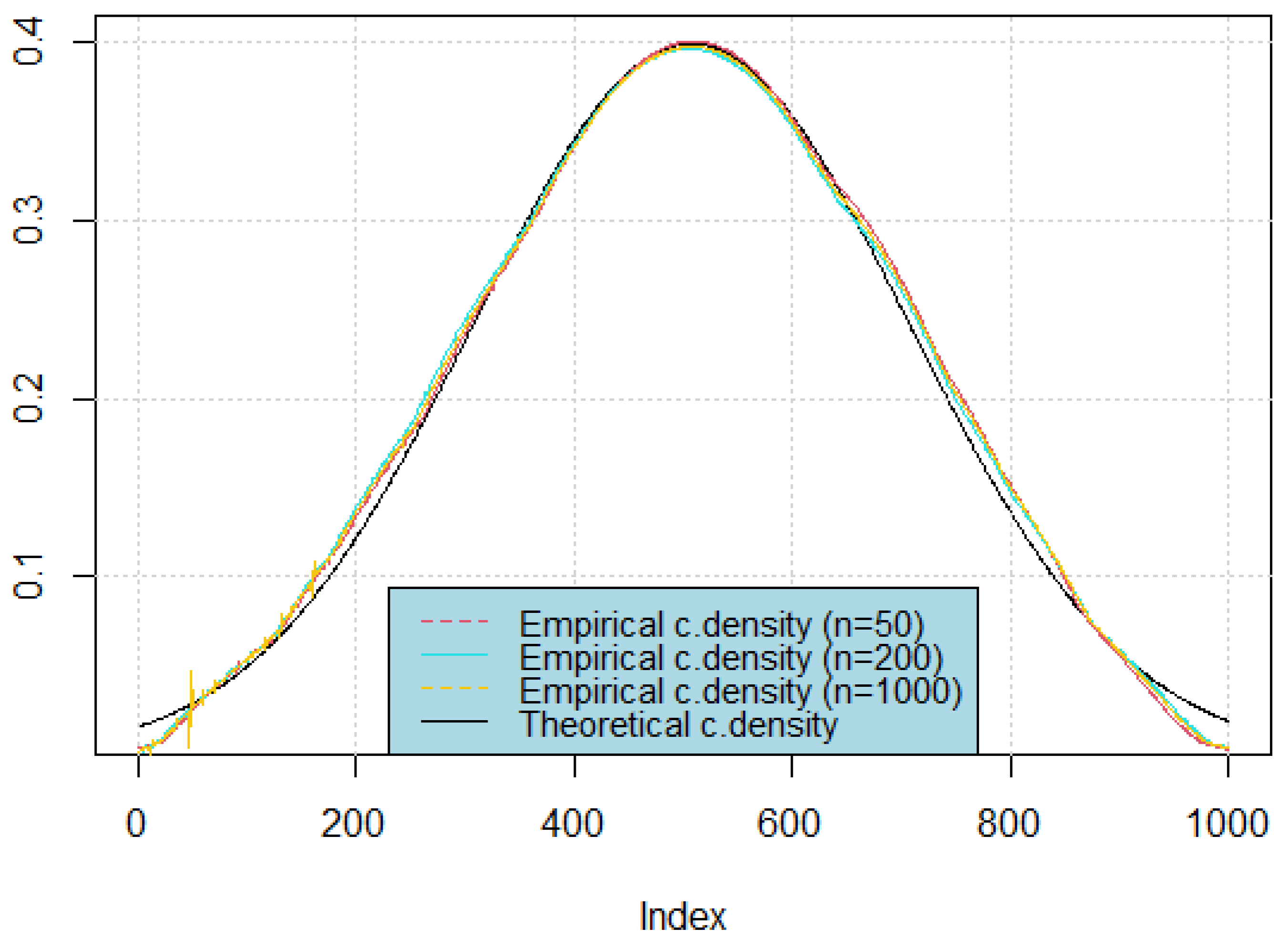
Figure 6.
Normal approximation of the conditional hazard function estimator.
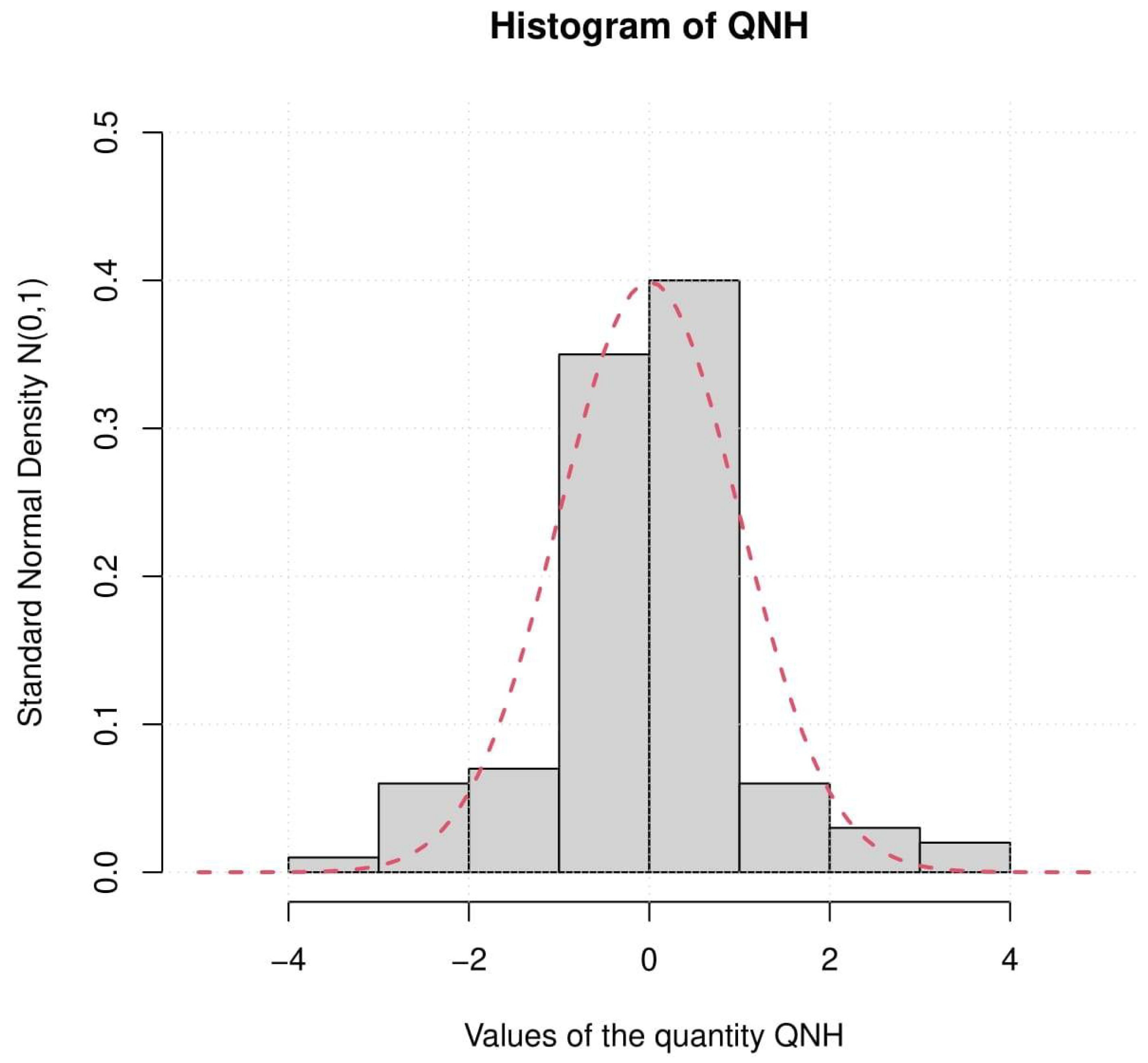
Figure 7.
Empirical and theoretical conditional hazard function estimation with confidence bounds.
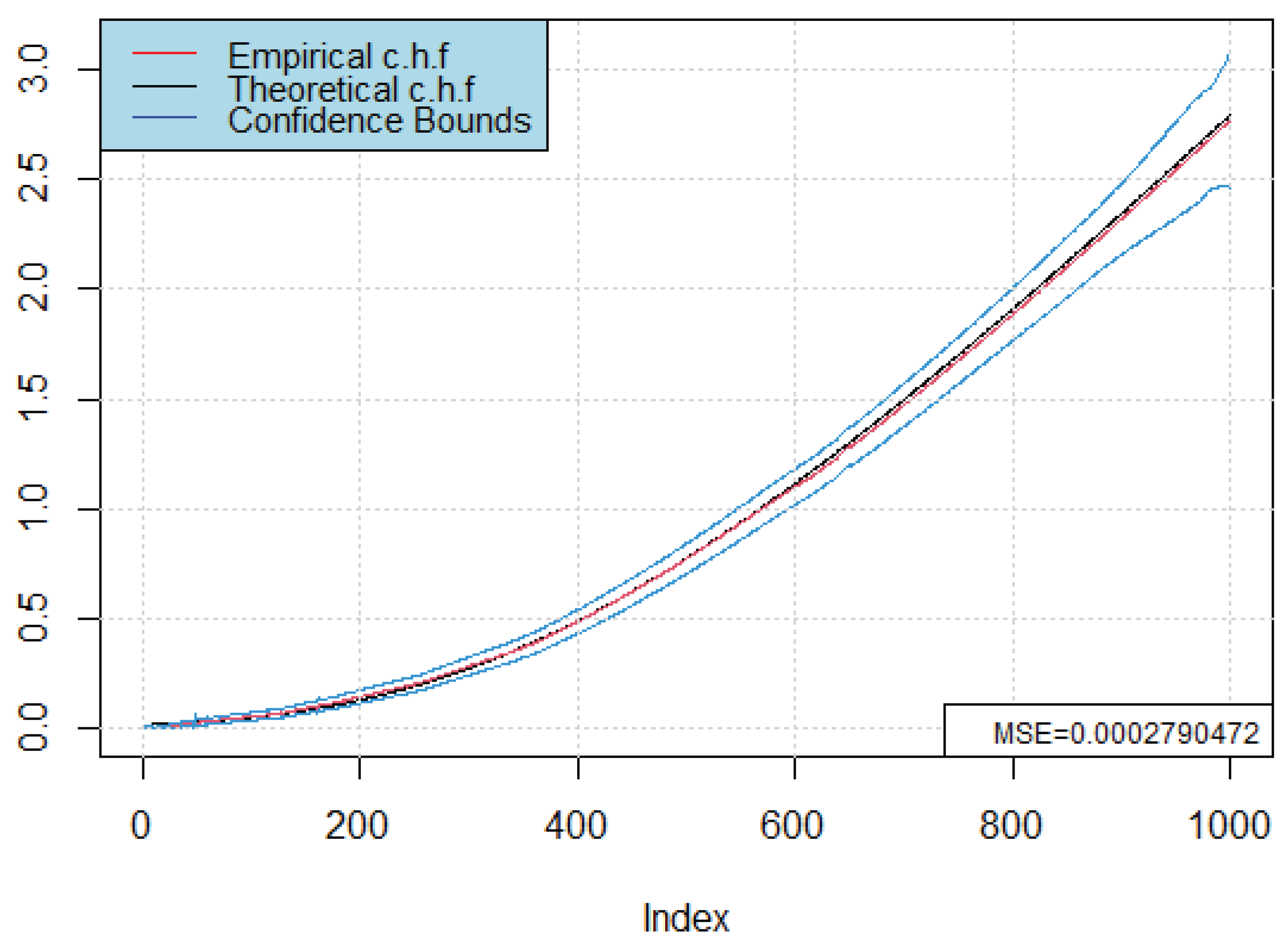

Table 1.
Mean square error of our estimators.
| Mean Square Error | n=50 | n=200 | n=1000 |
|---|---|---|---|
| MSE( ) | |||
| MSE( ) |
Disclaimer/Publisher’s Note: The statements, opinions and data contained in all publications are solely those of the individual author(s) and contributor(s) and not of MDPI and/or the editor(s). MDPI and/or the editor(s) disclaim responsibility for any injury to people or property resulting from any ideas, methods, instructions or products referred to in the content. |
© 2025 by the authors. Licensee MDPI, Basel, Switzerland. This article is an open access article distributed under the terms and conditions of the Creative Commons Attribution (CC BY) license (http://creativecommons.org/licenses/by/4.0/).
Copyright: This open access article is published under a Creative Commons CC BY 4.0 license, which permit the free download, distribution, and reuse, provided that the author and preprint are cited in any reuse.


