Submitted:
21 August 2025
Posted:
22 August 2025
You are already at the latest version
Abstract
Forecasting high-volume, univariate, and multivariate longitudinal data streams is a critical challenge in Big Data systems, especially with constrained computational resources and pronounced data variability. This paper addresses this challenge through the introduction of a dual-level contribution. First, we propose a theoretical framework for quantifying “data bigness” as a function of statistical, computational, and algorithmic complexity. This lens allows for more precise formalization of resource-bound analytics in dynamic environments. Second, we present the Adaptive High-Fluctuation Recursive Segmentation (AHFRS) framework, which leverages multivariate fluctuation statistics to construct compact, information-dense training subsets within bounded memory windows. Unlike static or recency-based methods, AHFRS dynamically selects historical segments with significant variance. This improves predictive signal retention under strict computational budgets. The framework is validated using synthetically generated longitudinal datasets across Finance, Retail, and Healthcare domains, each modeling domain-specific temporal dynamics while controlling for population heterogeneity. Forecasting is performed on a per-customer basis to simulate individualized inference under constrained memory conditions. Experimental results demonstrate that AHFRS consistently improves predictive performance across learning models and domains. This approach advances the theoretical modeling of data complexity and the design of adaptive, resource-efficient forecasting pipelines for real-world, high-volume data ecosystems. The proposed segmentation framework is validated on both real-world univariate and synthetic multivariate datasets. A univariate case study using Bitcoin hourly price data demonstrates early effectiveness of the model, which is then extended to multivariate domains in Finance, Retail, and Healthcare.
Keywords:
Univariate time series
; Multivariate time series
; Big Data analytics
; Recursive window segmentation
; High fluctuation
; Predictive modeling
; Data optimization
1. Introduction
The rapid increase in multivariate longitudinal data across industries has created a new era of big data analytics, presenting both vast opportunities and significant challenges. As data continuously expand in volume, velocity, and variety, traditional analytical frameworks often fail to address the complexities of dynamic real-world datasets [1,2]. The need for scalable, context-aware solutions to extract meaningful insights and improve predictive accuracy has become paramount [3]. Previous research advanced big data analytics by proposing quantitative definitions of "data bigness" and the "3Vs" framework (volume, velocity, variety) [4,5]. However, these approaches often overlook critical multivariate statistical properties such as covariance, skewness, and kurtosis [6,7]. Furthermore, existing segmentation algorithms designed for univariate scenarios struggle to adapt to the intricate interdependencies present in multivariate longitudinal datasets [8]. These limitations highlight the need for methodologies that capture the nuanced statistical variability of data while aligning with the unique requirements of various industries [3,9]. This paper builds on these foundations by introducing an enhanced adaptive segmentation framework that integrates statistical variability with traditional attributes of big data. Specifically, this paper refines the quantitative definition of "data bigness" introduced in [8] to include multivariate statistical measures. This enables dynamic computation of window sizes tailored to individual dataset characteristics [3,10]. This adaptive approach optimally combines high-fluctuation data segments with recent trends to form robust predictive datasets. This addresses computational constraints and the complexities of diverse industry applications [8,11]. The core contribution of this paper lies in the application of advanced multivariate statistical analysis to dynamically adjust segmentation processes. By incorporating measures such as mean vectors, covariance matrices, skewness, and kurtosis, the proposed methodology precisely models temporal and structural patterns across industries [6,7,12]. Empirical evaluations in finance, retail, and healthcare demonstrate significant improvements in the accuracy of forecasting, underscoring the scalability and effectiveness of the approach [13,14,15]. This work not only advances the theoretical understanding of data bigness but also provides a practical framework for Big Data analytics that bridges the gap between research and real-world applications. By offering scalable and context-aware solutions for multivariate longitudinal data challenges, this paper enables more informed decision-making and innovation across sectors [16].
Although this paper focuses on multivariate forecasting, the foundational segmentation framework is designed to operate both on univariate and multivariate longitudinal data. In prior work [8], we demonstrated that the AHFRS approach significantly improved forecasting performance for univariate financial time series (Bitcoin), even under strict processing constraints. This study generalizes that work, extending the methodology to multivariate contexts with domain-specific temporal characteristics and interdependencies.
2. Existing Literature Review: Big Data Definition
The explosion of data over recent decades has made Big Data a central focus of research and application across numerous fields. Despite its widespread use, the term "Big Data" often remains ambiguous, as multiple definitions attempt to capture its essential characteristics. This section critically reviews the evolution of Big Data definitions, their strengths, limitations, and relevance to contemporary analytics. This review identifies key gaps to establish a foundation for a precise, quantitative definition of "Big Data" that is tailored to modern data challenges.
2.1. Foundational Frameworks: The "3 Vs" Model
Doug Laney’s seminal "3 Vs" model, introduced in 2001, laid the groundwork for understanding Big Data [4]. This framework defined Big Data along three dimensions: Volume (the vast amounts of data generated), Variety (the diversity of data types), and Velocity (the speed at which data are produced and processed). These dimensions underscored the technological challenges of managing large-scale datasets and became a cornerstone in both academic and industrial contexts [4,17]. However, the "3 Vs" model has faced criticism for oversimplifying the complexities of modern data environments. Kitchin and McArdle (2016) argued that this framework overlooks ontological nuances of "Big Data," such as exhaustivity (comprehensive data capture), indexicality (real-time source alignment) and relationality (interconnected data flows) [10]. Their work expands the original framework by acknowledging the unique characteristics of contemporary data, particularly in domains like social media and geospatial systems [10,17]. This evolution reflects a growing demand for sophisticated models that capture the intricacies of modern data ecosystems.
2.2. Expanded Definitions: Moving Beyond the "3 Vs"
To address the limitations of the "3 Vs" model, researchers have proposed more comprehensive definitions of Big Data. De Mauro et al. (2016) highlighted infrastructural and computational challenges, defining "Big Data" as datasets "too large, too complex, and too fast" for traditional systems to process effectively [1]. This definition catalyzed the development of scalable architectures like Hadoop and Spark, which are now foundational in Big Data analytics [9]. Nonetheless, the absence of universally accepted thresholds for classifying data as "big" remains a challenge. Many definitions rely on arbitrary metrics, such as data volume in terabytes or petabytes, which vary depending on context and application [1,17]. This variability underscores the need for a universally applicable definition that incorporates both qualitative and quantitative criteria.
2.3. Industry-Specific Definitions: Real-Time Analytics and Decision-Making
In industry, Big Data definitions often cater to specific use cases, reflecting practical needs. Ajah and Nweke (2019) highlighted the transformative role of Big Data in enabling real-time analytics, allowing businesses to dynamically respond to market trends, customer behaviors, and emerging patterns [2]. This real-time capability is critical in sectors where timely insights drive competitive advantage. Gandomi and Haider (2015) extended the conversation by emphasizing the growing dominance of unstructured data—such as social media posts, images, and videos—which now constitutes the majority of Big Data [11]. Analyzing unstructured data presents challenges that require advanced algorithms and tools to extract actionable insights. This highlights the need for industry-specific definitions aligned with evolving data characteristics [2,11].
2.4. Critical Challenges and the Need for Standardization
Despite significant advancements, the field continues to grapple with key challenges. A notable issue is the lack of standardized thresholds for determining when data qualifies as "big." Existing definitions often use system-specific constraints, hindering the development of universal metrics [1,9]. Furthermore, as technology advances and data complexity increases, traditional frameworks may struggle to keep pace. De Mauro et al. (2016) and Kitchin and McArdle (2016) stressed that "Big Data" definitions must be refined to address emerging challenges like data quality, accessibility, and ethics [1,6]. The rise of artificial intelligence and machine learning further complicates this landscape, requiring definitions that consider privacy, governance, and ethical dimensions [2,9].
2.5. Toward a Quantitative and Contextual Understanding
The reviewed literature highlights a dynamic and evolving field, underscoring the need for more robust frameworks. While foundational models like the "3 Vs" remain relevant, they must be expanded to accommodate the growing complexity of modern data environments. A quantitative definition of "Big Data," which incorporates measurable parameters for data size, complexity, and variability, would clarify its academic and industrial applications. This review lays the groundwork for proposing such a definition, aimed at standardizing the understanding and management of Big Data. By addressing current gaps, this paper offers a structured, adaptable, and precise framework for meeting the demands of the digital age.
3. Data bigness: A statistical variability-based framework
Building on prior definitions (Section 2), this section enhances the definition of data bigness introduced by D. Fomo and A.-H. Sato in [18] by proposing a multi-dimensional framework to characterize "Big Data" more rigorously and quantitatively. Traditional definitions, often focused on the "3Vs" (Volume, Velocity, Variety), lack the nuance to capture the full range of modern data analysis challenges. This framework extends these concepts by integrating three crucial dimensions of complexity: Statistical, Computational, and Algorithmic (NP-Hard). Thus, "bigness" is evaluated not just by data scale (volume, velocity) or diversity (variety), but more holistically by its inherent statistical properties, required computational resources, and the intrinsic difficulty of analytical tasks. This comprehensive view provides a more operationally relevant and analytically insightful definition, especially for navigating challenges in data-intensive domains like finance, retail, and healthcare.
3.1. Multidimensional Quantitative Definition of Big Data
We propose that a dataset , in the context of a specific analytical task implemented via algorithm , qualifies as Big Data if it meets or exceeds predefined context-dependent thresholds () in at least one of the following complexity dimensions ():
Each dimension is defined more formally as follows:
3.1.1. Statistical Complexity ()
This dimension quantifies complexity from the dataset’s intrinsic statistical characteristics, particularly deviations from simplifying assumptions (like normality or independence) or the presence of high variability, heterogeneity, or instability. Such characteristics often necessitate more sophisticated or robust analytical methods. A composite measure, , is proposed in [18], integrating key multivariate statistical properties:
Where:
- : The norm of the estimated mean vector. Significant magnitude or temporal drift in can complicate modeling, especially in non-stationary contexts [6].
- : Absolute multivariate kurtosis, defined by K.V. Mardia in [7], assessing the "tailedness" and peakedness relative to a multivariate normal distribution. High kurtosis indicates heavy tails (leptokurtosis), suggesting a higher propensity for outliers or extreme events that can destabilize standard estimators and necessitate robust statistical approaches [23].
- Tr(): The trace of the covariance matrix, equivalent to the sum of the variances of individual variables . It provides a simple scalar summary of the total variance or dispersion within the dataset [28]. High total variance can be indicative of complexity, particularly in high-dimensional settings.
3.1.2. Computational Complexity ()
This dimension quantifies the practical resource requirements associated with executing algorithm on dataset , specifically processing time and memory (space). It directly reflects the computational burden and scalability challenges.
where:
- : A numerical representation of the algorithm’s asymptotic time complexity (e.g., mapping , , , to a monotonically increasing numerical scale). High time complexity signifies that execution time grows rapidly with data size n, potentially exceeding acceptable latency or processing windows [17,23,24].
The weights and permit balancing the relative importance of time versus memory constraints based on specific system limitations or application requirements.
3.1.3. Algorithmic (NP-Hard) Complexity ()
This dimension addresses the intrinsic computational difficulty of the analytical problem algorithm aims to solve, especially if the problem is in a computationally hard complexity class (e.g., NP-hard [25,26]). For such problems, finding an exact optimal solution is generally considered intractable for large input sizes within feasible time, necessitating heuristic or approximation strategies. Many core tasks in Big Data analytics including certain types of clustering, feature selection, graph partitioning, network analysis, and combinatorial optimization fall into this category.
where:
- : An indicator reflecting the complexity class of the problem solved by A. For instance, could be assigned a high value (e.g., 1) if the problem is NP-hard and typically requires non-exact methods for large instances encountered in Big Data, and a low value (e.g., 0) if the problem admits efficient polynomial-time algorithms.
This dimension highlights scenarios where the primary challenge stems from the combinatorial nature of the problem itself, demanding specialized algorithmic techniques beyond just scalable infrastructure.
3.2. Establishing Domain-Specific Thresholds () and Implication
It is essential to recognize that the thresholds (, , ) that delineate "Big Data" within this framework are not universal constants. Instead, they are context-dependent benchmarks established relative to domain norms, analytical objectives, available infrastructure, and current algorithmic advancements.
- Finance: Statistical thresholds () for high kurtosis might be benchmarked against historical crisis data [15,21]. Computational thresholds () could be dictated by latency requirements (e.g., algorithms slower than deemed too slow). NP-hard complexity () could be triggered by tasks like complex portfolio optimization [22,27,28].
- Retail: Statistical thresholds () might relate to identifying significant deviations in customer behavior [29]. Computational limits () could be set by the feasibility of daily analyses on massive transaction volumes (e.g., infeasible). NP-hard challenges arise in vehicle routing or large-scale clustering [30].
Defining appropriate thresholds requires careful consideration, empirical analysis, and domain expertise. This multi-dimensional framework practically guides the selection of appropriate analytical strategies. Diagnosing the dominant complexity source(s) leads to targeted interventions:
- High Algorithmic Complexity (): Requires shifting from exact methods to well-justified heuristics, approximation algorithms, randomized algorithms, or specialized solvers [32].
3.3. Contextualizing Statistical Complexity: Positioning within Existing Frameworks
Efforts to formalize complexity have yielded a wide variety of measures across disciplines, each grounded in specific theoretical frameworks and optimized for different modeling goals. Some aim to quantify the balance between order and randomness, others assess memory or predictability, and others reflect the difficulty of learning or compressing data. These perspectives have driven fundamental progress in physics, information theory, computational mechanics, and neuroscience.
This section situates the proposed measure within this broader methodological landscape. It does not attempt to generalize, replace, or outperform these well-established frameworks. Instead, it addresses a growing operational need to quantify statistical heterogeneity in large multivariate datasets in a computable, interpretable, and useful way for adaptive data handling under resource constraints.
Each of these frameworks depicted in Table 1 formalizes complexity within its respective theoretical domain. Some focus on intrinsic system structure, others on descriptive efficiency, and some on the hardness of learning or predicting under uncertainty. In contrast to these system-oriented or task-oriented metrics, is defined specifically to characterize segments of multivariate data that exhibit properties statistically “unfriendly” to modeling. These include:
- Elevated variance (trace or norm of the covariance matrix)
- Non-Gaussian behavior (skewness and kurtosis)
- Strong inter-variable correlation (covariance structure)
- Shifting distributional centers (mean norm)
Each component is a standard multivariate statistic, making transparent, scalable, and compatible with existing data preprocessing pipelines. Moreover, its weighted form enables domain customization, where weights can reflect analytic priorities (e.g., tail risk in finance or asymmetry in population health data). Rather than framing as a general-purpose statistical complexity measure, we position it as a task-aware diagnostic designed to flag data segments that are statistically complex in ways that impede efficient modeling. Key distinctions include:
- Objective: Classical complexity measures aim to understand system behavior; aims to support model selection and window adaptation.
- Granularity: Other measures operate at the level of entire systems or sequences; is local and segment-level.
- Actionability: Its values directly inform whether a dataset slice warrants specialized modeling strategies or resource allocation.
This makes particularly valuable in data-intensive applications such as real-time forecasting, anomaly detection, and adaptive sampling, where decisions must be informed by local statistical characteristics under strict processing budgets.
The concept of statistical complexity is not monolithic. It must be understood relative to what is being modeled, what constraints exist, and what outcomes are sought. While Kolmogorov complexity addresses informational minimalism, Excess Entropy captures structure, and DEC formalizes decision-making hardness, is designed to answer a different question: Is this segment of data statistically well-behaved enough for routine modeling, or does it require adaptive treatment? In answering that question, does not redefine statistical complexity; it retools it for analytics at scale.
3.4. Advantages of Our Proposed Multi-Dimensional Framework
This framework offers several significant advantages over traditional, often underspecified, "Big Data" definitions:
- Theoretical Rigor and Comprehensiveness: Provides a more complete, multifaceted, and conceptually sound basis for characterizing the challenges posed by modern datasets, grounded in statistics and computer science principles.
- Enhanced Interpretability: It clearly separates distinct sources of difficulty (statistical properties, resource demands, intrinsic problem hardness), allowing a more precise diagnosis of analytical bottlenecks.
- Actionable Analytical Guidance: It directly informs strategic decisions on selecting appropriate statistical methods, computational infrastructure, and algorithmic techniques tailored to the specific complexities encountered.
Adopting this multi-dimensional perspective can help the field develop a more standardized, insightful, and operationally useful understanding of "Big Data". This facilitates the development and application of more effective strategies for data analysis and robust data-driven decision-making in an increasingly complex data landscape.
4. Review of Big Data Analytics Challenges
Building on the multi-dimensional "data bigness" framework from Section 3 (characterizing statistical (), computational (), and algorithmic () complexities), this section examines specific, interconnected challenges in big data analytics. While the potential for deriving valuable insights from vast datasets is immense [40], realizing this potential is frequently hindered by obstacles stemming directly from the inherent characteristics of Big Data often summarized by the Vs: Volume, Velocity, Variety, and increasingly, Veracity and Value [41,42]. As highlighted, efficiently managing, processing, and extracting insights from massive, diverse, and rapidly generated datasets is a primary hurdle for organizations using big data for forecasting and strategic decisions. These challenges necessitate sophisticated analytical strategies and robust computational infrastructure.
4.1. Challenges Stemming from Statistical Complexity () and Data Veracity
A primary set of challenges arises from the intrinsic statistical properties and quality issues within Big Data. Common in many industries, multivariate longitudinal datasets often show significant non-stationarity, heterogeneity, and high statistical variability (including complex correlations, skewness, and kurtosis), which complicates using traditional models. Identifying and modeling these underlying structures requires advanced analytical approaches adaptable to local data characteristics.
Compounding this statistical complexity is the challenge of Data Veracity, ensuring the quality, accuracy, consistency, and trustworthiness of the data [41,42]. Big data, often aggregated from diverse sources, is frequently messy, with issues like incompleteness, noise, errors, inconsistencies, and duplication [42,43,44,45]. Poor data quality is a critical bottleneck, as it can lead to flawed analysis, unreliable conclusions, and poor decision-making [40,44,46]. Studies suggest a significant percentage of Big Data projects fail due to data quality management issues [46]. Addressing this requires robust data governance, rigorous (and potentially computationally intensive) data cleaning and preprocessing, and validation procedures [40,41,42,43,46]. However, automated cleaning techniques often struggle with the diversity and complexity of real-world datasets [43], necessitating human intervention and domain expertise [43].
Moreover, our prior work highlighted a challenge: balancing the capture of relevant historical patterns (e.g., high fluctuations or seasonality in older data) with an emphasis on recent trends, especially under strict data volume constraints. Naively discarding older data, a common approach to manage volume, can lead to a significant loss of information about long-term cycles or rare events crucial for accurate forecasting.
4.2. Challenges Stemming from Computational Complexity (), Volume, and Velocity
The defining characteristics of Volume and Velocity translate directly into significant computational hurdles. Organizations now grapple with petabytes or exabytes of data, rendering traditional storage solutions inadequate and requiring scalable infrastructure like cloud storage (e.g., Amazon S3, Google Cloud Storage, Microsoft Azure), data lakes, compression, and deduplication techniques [42,45,47]. The sheer volume strains processing capacity, impacting both time complexity () and space complexity (). Many standard algorithms, particularly traditional Machine Learning algorithms, scale poorly and become computationally prohibitive as data size grows [43,48].
The rapid rate at which data is generated (e.g., from IoT devices, social media) and needs processing demands real-time or near-real-time analytical capabilities [40,42]. This often necessitates stream processing frameworks (e.g., Apache Kafka, Apache Flink) over traditional batch processing, adding complexity and cost [40,42]. Efficiently collecting, processing (transforming, extracting), and analyzing these large, fast-moving datasets is a significant challenge [40,41]. Achieving true scalability requires efficient distributed computing techniques, parallel processing, data partitioning, and fault tolerance, which present their own implementation challenges [43,48]. System limitations, like maximum processable data volume (discussed in prior work), necessitate intelligent data reduction or selection to preserve information within computational budgets.
4.3. Challenges Stemming from Algorithmic Complexity ()
Beyond resource constraints, some Big Data analytics tasks, such as specific types of clustering, feature selection, optimization, or network analysis, are intrinsically difficult due to their underlying Algorithmic Complexity. Many such problems are NP-hard, meaning exact optimal solutions are generally intractable for large inputs within feasible timeframes. This necessitates the use of approximation algorithms, heuristics, or randomized methods, which trade optimality for computational feasibility. Recognizing and appropriately addressing this intrinsic hardness is crucial for selecting suitable analytical techniques.
4.4. Interrelated Challenges: Variety, Integration, Security, Value Extraction, and Skills
The aforementioned challenges are often compounded by other factors:
- Variety and Integration: Big Data encompasses diverse types (structured, unstructured, semi-structured) from multiple sources. Integrating these heterogeneous sources for analysis is challenging, sometimes requiring specialized tools (e.g., NoSQL databases [49]) and potentially leading to data silos that hinder comprehensive analysis [42,44,45,47].
- Security and Privacy: Protecting vast amounts of potentially sensitive data is paramount [40,41]. Concerns include data breaches, compliance with regulations (e.g., GDPR, CCPA), unauthorized access, and ensuring privacy throughout the data lifecycle [42,44,45,50]. Big Data environments, including IoT initiatives, increase the potential attack surface by introducing more endpoints [50]. Robust security measures like comprehensive data protection strategies, encryption, authentication, authorization, and strict, granular access control are essential but challenging to implement at scale [41,42,45,50,51].
- Value Extraction and Skills Gap: Extracting meaningful, actionable insights and generating tangible value from big data is the ultimate goal, yet it remains a significant challenge [41,51]. Furthermore, surveys indicate a lack of skilled personnel (e.g., data scientists) with the expertise to manage the infrastructure, apply advanced analytical techniques, and correctly interpret results is a major barrier to adoption [45,50]. Selecting the right tools and platforms is also crucial but complex, as no single solution fits all Big Data needs [40,44].
Addressing this complex web of challenges requires multifaceted solutions. Methodologies must be statistically robust, computationally scalable, algorithmically sophisticated, secure, and flexible. The adaptive segmentation framework proposed later contributes a strategy to navigate trade-offs between incorporating rich historical information (including fluctuations) and adhering to processing constraints. This enhances forecasting model effectiveness for complex multivariate big data.
5. Proposed Methodology: Adaptive High-Fluctuation Recursive Segmentation
5.1. Introduction and Context
To address the big data analytics challenges from Section 4, computational constraints () limiting processable data, statistical complexity () of multivariate longitudinal data and balancing recent trends with historical fluctuations, advanced data selection strategies are required for effective forecasting. A key issue is how to select the most informative subset of data as depicted in Figure 1. Naïve methods often rely solely on the most recent data points, discarding older but potentially important patterns [8]. This can lead to missed signals from significant past fluctuations. While data segmentation plays an important role, existing techniques have notable limitations in this context. To overcome these, we introduce a new method: the Adaptive High-Fluctuation Recursive Segmentation algorithm (AHFRS). This approach dynamically combines statistical variability analysis with likelihood-based segmentation to construct a highly optimized forecasting dataset.
5.2. Review of Baseline Segmentation Approaches and Their Limitations
To contextualize our method’s contributions, we review two common baseline approaches for processing time series data streams (Fixed-Size Sliding Windows and ADWIN). We then evaluate their limitations regarding our objective: optimizing datasets for multivariate longitudinal forecasting under processing constraints while preserving historical context.
5.2.1. Fixed-Size Sliding Windows
Overview: This approach, arguably the most conventional and straightforward, applies a sliding window of fixed length over the time series. As new observations arrive, the window advances by one step, and forecasting models are trained or updated using only the data within the current window.
Relevance and Limitations in Multivariate Longitudinal Big Data: Fixed-size windows naturally extend to multivariate settings by including the most recent multivariate observations. However, their main limitation is their non-adaptive nature. Multivariate longitudinal datasets, particularly in domains such as finance, retail, and healthcare, are typically non-stationary, exhibiting dynamic trends, evolving volatility, and varying seasonality [9,12,15,29]. A static window size cannot accommodate these fluctuations effectively. Short windows may fail to capture long-term dependencies or seasonal cycles present in the historical data. While long windows, conversely, risk smoothing over recent changes, reducing responsiveness and adaptability. Most importantly, this approach discards all observations older than , thereby neglecting potentially valuable historical segments. This omission is problematic when earlier fluctuations contain significant predictive value—an insight our method leverages [8].
5.2.2. ADWIN (Adaptive Windowing)
Overview: ADWIN [52] is a parameter-free, adaptive algorithm developed to detect concept drift in data streams by monitoring changes in the mean or distribution. It maintains a dynamic window of recent data and reduces its size when a statistically significant difference is observed between sub-windows. For multivariate data, ADWIN typically requires modification, such as monitoring a univariate proxy derived from the multivariate input (e.g., Mahalanobis distance, model prediction error, or combined variance metrics).
Relevance and Limitations in Multivariate Longitudinal Big Data: Compared to fixed-size windows, ADWIN introduces adaptivity by reacting to changes in data distribution and is thus a more sophisticated baseline. However, its design and objectives are not fully aligned with the requirements of our task, for the following reasons:
- ADWIN is optimized for detecting recent changes and retaining data from the current distribution. In contrast, our approach identifies historically significant segments with pronounced statistical fluctuation and integrates them with recent observations to form a forecasting-optimized dataset.
- Upon detecting change, ADWIN discards the older portion of its window to maintain adaptability. In contrast, our method explicitly retrieves and reuses historical segments, selecting those with statistically significant fluctuation for inclusion in the forecasting dataset. Thus, where ADWIN forgets, our approach remembers selectively.
- ADWIN primarily bases its adaptation on changes in means or simple distributional statistics. Our method incorporates a richer multivariate statistical characterization, leveraging higher-order moments such as skewness and kurtosis. This design allows our method to adapt to complex features like volatility, asymmetry, and tailedness, which are important in real-world, high-dimensional forecasting across diverse industries [7,21,53].
In summary, while both Fixed-Size Sliding Windows and ADWIN serve as important baselines, they are not fully equipped to address the dual challenges of statistical adaptivity and historical context utilization under constrained conditions. Our method overcomes these limitations by using likelihood-ratio segmentation to identify significant past fluctuations. It also utilizes higher-order statistical adaptation for window sizing and segment replacement, and explicitly constructs an optimized forecasting dataset by selectively combining historical and recent data.
5.3. Foundational Recursive Segmentation (Likelihood Ratio)
The core segmentation technique employed in our proposed architecture (Figure 2) for identifying high-fluctuation segments is a likelihood-based recursive segmentation algorithm, originally proposed by Sato [54] and used in our prior work [8]. This method builds on principles from change point detection [55,56], aiming to detect time points where the statistical properties of a time series exhibit abrupt shifts.
Let us consider a multivariate time series segment of length , represented by its -dimentional fractional changes , where and (with ). For each candidate split point , where denotes the minimum segment length, the algorithm computes a likelihood ratio . This statistic compares the likelihood under a two-segment model (with a split at time t) against a single-segment model.
Assuming approximate multivariate normality within segments, the statistic is computed via the determinants of the estimated covariance matrices for the entire segment (), the left segment (), and the right segment (), as detailed in [8] and [18]:
The covariance matrices are estimated from as:
The optimal split point is identified as the value of t that maximizes :
larger indicates a more statistically significant deviation between sub-segments, suggesting a high fluctuation change point. This binary splitting is applied recursively to the resulting segments. The process terminates when for a potential split falls below a predefined statistical significance threshold, typically based on the distribution [8]. The result is a partition of the series into statistically homogeneous segments, denoted by the set of boundaries .
5.4. Adaptive Window Size Determination
A central innovation introduced in [18] is the adaptive replacement of the fixed window percentage used in [8] with a dynamically computed window size, denoted as . This addresses the limitation that a fixed percentage () may not adequately capture the statistical stability or variability of the recent segment (length ).
The method identifies the largest, most recent, contiguous sub-segment within that shows high internal statistical similarity. The segment is assumed to be relatively stable and less informative compared to high-fluctuation historical periods.
For all possible partitions of into left (, from start to time t) and right (, from to end), two similarity metrics are computed:
- Preliminary Similarity () which captures differences in central tendency and overall variance:where and represent the norm of the mean vector and the trace of the covariance matrix for data segment respectively. and represent the same for data segment .
- Detailed Similarity () which measures difference in higher-order moments using the composite variability metric defined in [18], which includes skewness and kurtosis and ensures that the two segments are also aligned in their distributional characteristics, such as shape, asymmetry, and tail behavior [7,21,54]:where and represent the weighted aggregation composite metrics (defined in [18]) for data segment and respectively.
The partition that minimizes the combined similarity score constitutes the final window size () which is computed as follows:
The argmin operation identifies the specific data subset within the Top Subsets that yields the minimum combined similarity score. In this context, Top Subsets represents a set of candidate data segments derived from that have the lowest preliminary similarity (), suggesting high internal statistical stability. The function returns the length (number of observations) of the data subset.
The adaptive percentage is then defined as:
which reflects the fraction of considered statistically stable and subject to replacement.
5.5. High-Fluctuation Segment Selection and Optimal Dataset Construction
With the adaptive percentage computed, the algorithm constructs the optimized dataset by incorporating relevant historical context as depicted in Figure 3.
- Target Set for Segmentation (): Constructed by combining the full past segment of size with the earliest portion of the recent segment of length :
- Recursive Segmentation: Apply the likelihood-ratio segmentation algorithm (Section 5.3) on , yielding a set of statistically significant boundaries:
- Top-k Segment Selection: Rank boundaries by descending and select the top k. For each , extract a segment around it. The value of k and chunk sizes are chosen such that:
- Optimal Dataset Construction:
This ensures retains the original window size while integrating statistically significant historical fluctuations.
5.6. Advantages and Scalability
The adaptive window segmentation algorithm presented here and summarized in Figure 4 is designed with scalability as a key consideration, making it suitable for large, high-dimensional datasets typical in big data scenarios. Computationally intensive aspects, like recursive segmentation and calculating multivariate statistical properties (covariance, skewness, kurtosis), can significantly benefit from parallel execution. By distributing these computations across multiple processing cores or nodes within a cluster, the overall runtime can be substantially reduced.
For potential real-time or near-real-time applications, the methodology can be further optimized by leveraging distributed computing frameworks like Apache Spark or Hadoop [23,47]. These platforms enable efficient data partitioning, allowing independent processing of data segments before merging the final segmentation results. This parallelization capability is particularly advantageous in data-intensive domains such as finance and healthcare, where rapid data ingestion and timely analysis are often critical. Further investigation into implementing and benchmarking the algorithm within these distributed frameworks is warranted to empirically validate its scalability across diverse, large-scale datasets [18].
6. Evaluation Across Univariate and Multivariate Forecasting
This section presents the empirical validation of the AHFRS framework across both univariate and multivariate longitudinal time series scenarios. We begin by evaluating performance on a real-world univariate financial dataset, followed by assessments on synthetically generated multivariate datasets simulating domain-specific temporal patterns in Finance, Retail, and Healthcare.
6.1. Univariate Forecasting: Bitcoin Case Study
This experiment evaluates the performance of AHFRS in a univariate forecasting context using hourly Bitcoin price data. The goal is to assess the impact of statistically guided segmentation on forecasting accuracy under memory constraints.
6.1.1. Dataset and Forecast Objective
The dataset contains 37,196 hourly Bitcoin Weighted Price values (USD) spanning the period 2017-01-01 to 2021-03-30. The time series exhibits complex non-stationarity, volatility clusters, and seasonal structures common in high-frequency financial data. The forecasting target is the period 2021-03-01 to 2021-03-30. To simulate operational constraints, the training dataset size is limited to observations—approximately 40% of the full history. This constraint is applied uniformly across both univariate and multivariate evaluations.
6.1.2. Experimental and Environment Setup
The Adaptive High-Fluctuation Recursive Segmentation (AHFRS) algorithm identifies segments with high statistical complexity from earlier history and combines them with a proportion of the most recent data. This composite training set is constructed such that its size remains within the constraint.
Suppose that univariate time series . For univariate time series, the statistical complexity metrics Eq. (2) are simplified as:
- Mean norm becomes scalar mean .
- Covariance matrix norm is reduced to sample variance .
- Skewness and kurtosis are, respectively, reduced to their standard univariate forms as and .
- Trace of covariance matrix is equivalent to the sample variance .
The weights for this univariate Bitcoin case study were determined through empirical simulations on prior data. We set , , , and . This weighting scheme emphasizes the higher-order moments, skewness and kurtosis. This is crucial for financial time series like Bitcoin, which are characterized by significant non-Gaussian behavior, fat tails, and abrupt, extreme price fluctuations that often hold key predictive information for market volatility. By contrast, lower weights for the mean and variance acknowledge that their contribution to identifying critical high-fluctuation periods is less pronounced in highly non-stationary and volatile financial contexts, enabling the algorithm to focus on segments with genuinely significant deviations.
As our proposed algorithm, segments are identified using a recursive likelihood-ratio test defined in Eqs. (10) to (12) which for univariate dataset are simplified as follow:
The variances are estimated from as:
DynamicWindow ComputationHere, , , and are the sample means of the entire dataset, the left segment, and the right segment, respectively. The optimal split point is still identified as the value of t that maximizes , as per Eq. (12). This adaptation allows the recursive segmentation process to accurately identify statistically significant change points in univariate data streams.
The top-K historical segments are selected and combined with the dynamically computed latest of data to form the final training window. Forecasting is performed using the Holt-Winters exponential smoothing method configured as:
- Trend: multiplicative
- Seasonal: multiplicative
- Seasonal period: 365 (to capture daily seasonal cycles)
While the Holt-Winters exponential smoothing model is not inherently designed to capture the high volatility and non-linear dynamics typical of financial time series such as cryptocurrency prices, it is employed in this univariate evaluation as a deliberately constrained forecasting setup. The objective is not to achieve state-of-the-art predictive performance, but rather to isolate and quantify the contribution of the proposed AHFRS segmentation strategy within a consistent and controlled modeling framework. A baseline model using the most recent points without segmentation (“No Segmentation”) is used for comparison.
6.1.3. Forecasting Results
- A.
-
Dynamic Window ComputationTo comply with the system-imposed memory constraint of time steps, the AHFRS framework constructs a training dataset by combining two complementary segments:
- : the most recent 14,288 observations, representing (1 – 24.62%) of the memory budget , and
- : a set of non-contiguous high-fluctuation historical segments totaling 4,668 observations, accounting for the remaining 24.62%.
These high-fluctuation segments are identified using the likelihood ratio–based recursive segmentation method developed in our earlier work. This approach partitions the time series into statistically homogeneous intervals by computing likelihood ratios between adjacent windows and selecting breakpoints where a significant statistical shift is detected. The segments are then ranked by their fluctuation intensity, and the top-K segments are chosen based on their relative contribution to the total variability, all while respecting the global memory constraint .Figure 5 illustrates this segmentation layout for the univariate Bitcoin dataset. At the end of the series, the contiguous recent segment provides short-term contextual information. Interleaved across the earlier timeline are the selected high-variability segments , which capture historically significant behavioral shifts. The combination ensures that the training dataset contains both up-to-date signals and long-range fluctuation patterns that might otherwise be excluded under recency-based schemes. This segmentation strategy distinguishes AHFRS from conventional sliding window methods. Instead of discarding older data outright, AHFRS selectively incorporates historically significant segments based on structural changes in the series. This dynamic windowing capability allows the framework to construct a statistically optimized and computationally feasible training dataset that retains both short-term trends and long-term variability patterns critical to accurate forecasting. - B.
-
Forecasting Generation and Evaluation MetricsThe forecasting process involves training the Holt-Winters exponential smoothing model (configured as detailed in Section 6.1.2) on the respective training datasets: either the ’No Segmentation’ baseline (the most recent observations) or the ’AHFRS-enhanced’ dataset (). Once trained, the model generates multi-step-ahead predictions for the defined forecast horizon, which is the period 2021-03-01 to 2021-03-30 for the Bitcoin dataset. These predicted values, alongside the actual test data, are visually presented in Figure 6.Figure 6 illustrates the actual Bitcoin Weighted Price (TEST Data), the predictions from the ’No Segmentation’ baseline, and the predictions from the AHFRS-enhanced approach for the evaluation period. It highlights how the AHFRS framework leads to predictions that more closely track the actual price movements compared to the baseline. To quantitatively assess and compare the accuracy of these generated forecasts, we utilize three well-established metrics:
- Root Mean Squared Error (RMSE):
- Mean Absolute Error (MAE):
- Mean Absolute Percentage Error (MAPE):
Where m is the number of predictions, is the actual value for the i-th prediction, and is the predicted value for the i-th prediction. - C.
-
Performance SummaryThe univariate forecasting results provide strong empirical evidence of the AHFRS framework’s effectiveness in memory-constrained environments. By combining recent data with historically significant, high-fluctuation segments, the training dataset constructed by AHFRS achieves superior statistical diversity and predictive quality compared to a purely recent-window baseline.As shown in Table 2, the AHFRS-enhanced configuration yields consistent improvements across all three evaluation metrics:
- RMSE is reduced from 5743.12 to 4517.31, reflecting a 21.34% improvement,
- MAE drops from 4916.20 to 3553.85, a 27.71% improvement,
- MAPE decreases from 8.69% to 6.33%, representing a 27.15% relative reduction.
These gains highlight the forecasting benefits of retaining select, high-fluctuation historical segments—rather than relying solely on recency—especially in volatile time series contexts like cryptocurrency pricing. The forecasting model used in this univariate scenario is the Holt-Winters exponential smoothing method, configured with multiplicative trend and seasonality. Notably, despite the model’s relative simplicity, the predictive performance is significantly enhanced when paired with AHFRS, highlighting the importance of adaptive, informative input segmentation over model complexity alone.In summary, AHFRS significantly boosts univariate prediction accuracy under strict computational constraints. These findings affirm the framework’s relevance and lay the empirical foundation for its subsequent application to multivariate forecasting.
6.2. Multivariate Forecasting
We now evaluate AHFRS in multivariate contexts using synthetic datasets that simulate real-world dynamics in three domains: Finance, Retail, and Healthcare. The empirical evaluation of the AHFRS framework (Section 5) is designed to test its ability to enhance multivariate forecasting in resource-constrained environments. While the "data bigness" framework (Section 3) models statistical (), Computational (), and Algorithmic () complexity, this evaluation isolates as the primary constraint. We assess how effectively AHFRS extracts forecasting value when limited by strict computational constraints on data volume and processing throughput.
6.2.1. System Constraint and Forecasting Objective
Modern data-driven systems in finance, retail, and healthcare often face architectural limits in memory, computation, and latency. These limitations impose practical upper bounds on the historical data available for model training and inference. We define this constraint through a fixed, per-entity training window , representing the maximum allowable volume of past observations that may be processed for forecasting.
To ensure comparability with the univariate case, we apply the same training data constraint of of full historical observations. While multivariate series contain additional variables per time step, the constraint reflects a system-level limitation on the number of observations (rows) that can be stored or processed, rather than the total number of data values. This design choice allows consistent evaluation of AHFRS performance across both data modalities, isolating the effect of segmentation strategy rather than varying memory budgets.
Each of the three domain-specific datasets (Finance, Retail, and Healthcare) used in this paper contains 100 customers, with 2,282 daily multivariate records per customer. To simulate -bounded environments, we cap the training data per customer at records, precisely 40% of their historical timeline. The forecasting target representing the next 46 observations (5% of ), a horizon aligned with operational lead times in most predictive systems.
The core hypothesis tested in this setting is that not all historical data within are equally informative. The AHFRS algorithm constructs an optimized training subset by identifying segments with high informational density based on multivariate feature space fluctuations. AHFRS aims to outperform naïve recency-based strategies under identical volume constraints, thus demonstrating better use of the same data budget.
6.2.2. Domain-Specific Synthetic Datasets Definition
To ensure control, reproducibility, and domain diversity, we utilize three synthetically generated, yet statistically realistic, multivariate time series datasets, each aligned with a key real-world application domain:
-
Finance Dataset: Features include age, income, credit_score, loan_amount,loan_duration_months, interest_rate, default_risk_index.It simulates financial volatility, abrupt credit score shifts, and latent risk cycles.
-
Retail Dataset: Features include age, spending_score, number_of_purchases,average_purchase_value, churn_likelihood.It embeds patterns of consumer engagement, reactive purchase bursts, and promotional seasonality.
- Healthcare Dataset: Features include age, bmi, blood_pressure, cholesterol_level, exercise_hours_per_week, disease_risk_score. It models longitudinal health trajectories with gradual physiological changes and sporadic clinical risk spikes.
Each dataset maintains the same structural format and customer indexation, enabling direct performance comparisons while controlling for population heterogeneity. The synthetic design incorporates varying levels of skewness, kurtosis, and inter-feature covariance to provide AHFRS with meaningful statistical landscapes for segmentation.
Using synthetic datasets and focusing on stems from four key methodological priorities: (1) Controlled Evaluation under Fixed Constraints; (2) Cross-Domain Generalization with Common Cohort; (3) Reproducibility and Ethical Neutrality; (4) Complexity-Oriented Dataset Engineering.
6.2.3. Experimental and Environment Setup
- A.
- Comparative Method: Latest- Baseline The Latest- strategy represents a common industry practice where the model is trained on the most recent observations. This method assumes that recent data contains the most relevant patterns, but it discards older segments that may contain valuable structural information.
- B.
-
Evaluation Metrics and Model Selection RationaleForecasting performance is evaluated using RMSE, MAE, and MAPE. These metrics are first computed for each individual customer i and then averaged across all customers to derive consolidated performance measures (Mean_RMSE, Mean_MAE, and Mean_MAPE).Where is the number of predictions for customer i, is the actual value, is the predicted value, and N is the total number of customers.We conducted experiments using two tree-based ensemble learning methods: Random Forest Regressor (RF) and Gradient Boosting Regressor (GB). These non-parametric models are robust to non-linearity and heterogeneity, common in real-world data [57,58]. Their effectiveness is well-documented in finance [59,60], healthcare [61,62], and retail [63,64]. They are also computationally tractable and compatible with distributed frameworks like Spark and Hadoop [57,65], making them suitable for -constrained pipelines.
6.2.4. Results and Discussion
- A.
-
Industry-Specific Dynamic window computationFigure 7 illustrates the average proportion of the dynamic window selected by AHFRS across the three industries. The variation (Finance: 18.06%, Retail: 25.07%, Healthcare: 24.1%) highlights AHFRS’s dynamic adjustment based on statistical variability. This aligns with the data bigness model, where statistical complexity () interacts with resource constraints (). In industries like Finance, with abrupt shifts, the model selects concise, fluctuation-rich segments. Conversely, domains like Retail and Healthcare, with more gradual shifts, warrant longer segments.
- B.
-
Comparative Forecasting PerformanceTable 3 presents the comparative forecasting performance of RF and GB models under baseline and AHFRS-enhanced regimes. Key observations:
- Substantial Accuracy Gains with AHFRS: Across all industries and metrics, models trained using AHFRS-selected windows consistently outperform their baseline counterparts. For example, in the Finance industry, the RF model’s Mean_RMSE decreases from 0.72 (baseline) to 0.27 with AHFRS—a relative reduction of over 62.5%.
- Retail Domain Sensitivity: Despite already low error values in the retail baseline, AHFRS delivers notable improvements, emphasizing its efficacy even in domains with high-frequency and potentially noisy data.
- Robustness in Healthcare: The Healthcare dataset benefits markedly from AHFRS segmentation. RF’s Mean_MAPE improves from 15.83% to 5.96%, enhancing reliability in critical health forecasting.
- Model-Agnostic Benefits: Both RF and GB models benefit from AHFRS, suggesting the strategy enhances predictive capacity through upstream data selection, independent of the downstream model architecture.
6.2.5. Summary of Evaluation
This evaluation strongly supports our core hypothesis: intelligent, statistically guided segmentation under volume-based computational constraints can significantly enhance multivariate longitudinal forecasting. The AHFRS framework demonstrates:
- Dynamic Adaptability: Selection of optimal historical windows varies by industry, highlighting that effective forecasting under constrained resources requires context-sensitive segmentation.
- Consistent Predictive Improvements: Across all industries, AHFRS-enhanced training sets yield lower forecasting errors.
- Model-Independent Gains: The segmentation benefits are robust across both RF and GB models, affirming the general applicability of AHFRS.
These findings underscore the practical utility of the AHFRS framework in Big Data environments where processing volume must be minimized while preserving predictive performance.
7. Conclusion
This paper introduces the Adaptive High-Fluctuation Recursive Segmentation (AHFRS) framework as a robust solution for accurate univariate and multivariate longitudinal forecasting under computational constraints—a critical and pervasive challenge in big data systems across finance, healthcare, and retail. Based on a multidimensional concept of "data bigness" that formalizes statistical (), Computational (), and Algorithmic () complexities, our approach focuses on as the primary constraint in this evaluation. Using a carefully constructed empirical design with synthetic datasets (engineered to capture each industry’s statistical features and temporal dynamics), we validate AHFRS’s ability to dynamically identify and use high-information segments within constrained training buffers (). By selectively combining significant historical segments with recent data, AHFRS constructs optimally informative training windows. These yield superior forecasting performance (RMSE, MAE, MAPE) compared to common recency-based strategies.
Key findings demonstrate that:
- Dynamic adaptability in historical window sizing, guided by statistical variability, significantly improves forecast accuracy over fixed-length or naively adaptive baselines.
- AHFRS consistently reduces forecasting error across all three industries, with reductions in Mean_RMSE reaching up to 62.5% in finance and Mean_MAPE improvements exceeding 10 percentage points in healthcare.
- The framework’s effectiveness is model-agnostic, delivering performance gains across both Random Forest and Gradient Boosting regressors without relying on architecture-specific optimizations.
- Most importantly, AHFRS adheres to the imposed processing budget (), thus validating its scalability and practicality in real-world resource-constrained analytical environments.
These outcomes establish AHFRS as an operational strategy for big data forecasting, not just a statistical segmentation technique, as it maximizes predictive utility per unit of computational effort. It connects the theoretical framework with tangible, domain-versatile forecasting improvements, offering a blueprint for designing intelligent data preprocessing pipelines under resource constraints. Future work will extend the AHFRS methodology to real-time and streaming contexts, integrating it with distributed computing platforms such as Apache Spark to support high-throughput deployments. Furthermore, exploring its synergy with deep learning models—especially in scenarios with sufficient label density and tolerable latency—may unlock even greater accuracy in high-frequency forecasting.
Ultimately, this paper contributes a scalable, statistically grounded, and empirically validated framework that advances multivariate big data analytics, offering both theoretical insight and practical forecasting value.
References
- De Mauro, A.; Greco, M.; Grimaldi, M. A Formal Definition of Big Data Based on its Essential Features. Libr. Rev. 2016, 65, 122–135. [CrossRef]
- Ajah, I.A.; Nweke, H.F. Big Data and Business Analytics: Trends, Platforms, Success Factors and Applications. Big Data Cogn. Comput. 2019, 3, 32. [CrossRef]
- Lee, I. Big Data: Dimensions, evolution, impacts, and challenges. Bus. Horiz. 2017, 60, 293–303. [CrossRef]
- Laney, D. 3D Data Management: Controlling Data Volume, Velocity, and Variety. META Group, Inc., 2001.
- Laney, D. 3D Data Management: Controlling Data Volume, Velocity, and Variety. META Group Research Note, Feb. 6, 2001.
- Wang, X.; Liu, J.; Zhu, Y.; Li, J.; He, X. Mean Vector and Covariance Matrix Estimation for Big Data. IEEE Trans. Big Data 2017, 3, 75–86. [CrossRef]
- Mardia, K.V. Measures of Multivariate Skewness and Kurtosis with Applications. Biometrika 1970, 57, 519–530. [CrossRef]
- Fomo, D.; Sato, A. High Fluctuation Based Recursive Segmentation for Big Data. In Proceedings of the 2024 9th International Conference on Big Data Analytics (ICBDA), Tokyo, Japan, 8–10 March 2024; pp. 358–363.
- De Mauro, A.; Greco, M.; Grimaldi, M. What is Big Data? A Consensual Definition and a Review of Key Research Topics. In Proceedings of the 4th International Conference on Integrated Information, Madrid, Spain, 1–4 September 2014.
- Kitchin, R.; McArdle, G. What makes Big Data, Big Data? Exploring the ontological characteristics of 26 datasets. Big Data Soc. 2016, 3, 2053951716631120. [CrossRef]
- Gandomi, A.; Haider, M. Beyond the hype: Big Data concepts, methods, and analytics. Int. J. Inf. Manag. 2015, 35, 137–144. [CrossRef]
- Schüssler-Fiorenza Rose, S.M.; Contrepois, K.; Moneghetti, K.J.; et al. A Longitudinal Big Data Approach for Precision Health. Nat. Med. 2019, 25, 792–804. [CrossRef]
- Seyedan, M.; Mafakheri, F. Predictive Big Data analytics for supply chain demand forecasting: Methods, applications, and research opportunities. J. Big Data 2020, 7, 53. [CrossRef]
- Torrence, C.; Compo, G.P. A Practical Guide to Wavelet Analysis. Bull. Am. Meteorol. Soc. 1998, 79, 61–78.
- Bollerslev, T. Generalized Autoregressive Conditional Heteroskedasticity. J. Econom. 1986, 31, 307–327. [CrossRef]
- Bhandari, A.; Rahman, S. Big Data in Financial Markets: Algorithms, Analytics, and Applications; Springer Nature: Cham, Switzerland, 2021.
- Bhosale, H.S.; Gadekar, D.P. A Review Paper on Big Data and Hadoop. Int. J. Sci. Res. Publ. 2014, 4, 1–8.
- Fomo, D.; Sato, A.-H. Enhancing Big Data Analysis: A Recursive Window Segmentation Strategy for Multivariate Longitudinal Data. In Proceedings of the 2024 IEEE International Conference on Big Data (BigData), Washington, DC, USA, 15–18 July 2024; pp. 870–879.
- Jolliffe, I.T. Principal Component Analysis, 2nd ed.; Springer: New York, NY, USA, 2002.
- Brys, G.; Hubert, M.; Struyf, A. A robust measure of skewness. J. Comput. Graph. Stat. 2004, 13, 996–1017. [CrossRef]
- Kim, T.H.; White, H. On more robust estimation of skewness and kurtosis: Simulation and application to the S&P 500 index. Finance Res. Lett. 2004, 1, 56–73. [CrossRef]
- Markowitz, H. Portfolio selection. J. Finance 1952, 7, 77–91. [CrossRef]
- Hashem, I.A.T.; Yaqoob, I.; Anuar, N.B.; Mokhtar, S.; Gani, A.; Khan, S.U. The rise of Big Data on cloud computing: Review and open research issues. Inf. Syst. 2015, 47, 98–115. [CrossRef]
- Cormen, T.H.; Leiserson, C.E.; Rivest, R.L.; Stein, C. Introduction to Algorithms, 3rd ed.; MIT Press: Cambridge, MA, USA, 2009.
- Garey, M.R.; Johnson, D.S. Computers and Intractability: A Guide to the Theory of NP-Completeness; W. H. Freeman: San Francisco, CA, USA, 1979.
- Sipser, M. Introduction to the Theory of Computation, 3rd ed.; Cengage Learning: Boston, MA, USA, 2012.
- Bienstock, D. Computational complexity of analyzing credit risk. J. Bank. Finance 1996, 20, 1233–1249. [CrossRef]
- Hirsa, A. Computational Methods in Finance, 2nd ed.; CRC Press: Boca Raton, FL, USA, 2016.
- Sabbirul, H. Retail Demand Forecasting: A Comparative Study for Multivariate Time Series. arXiv 2023, arXiv:2308.11939.
- Hillier, F.S.; Lieberman, G.J. Introduction to Operations Research, 10th ed.; McGraw-Hill: New York, NY, USA, 2014.
- Gusfield, D. Algorithms on Strings, Trees, and Sequences: Computer Science and Computational Biology; Cambridge Univ. Press: Cambridge, U.K., 1997.
- Vazirani, V.V. Approximation Algorithms; Springer: New York, NY, USA, 2001.
- López-Ruiz, R.; Mancini, H.L.; Calbet, X. A statistical measure of complexity. Phys. Lett. A 1995, 209, 321–326.
- Feldman, D.P.; Crutchfield, J.P. Measures of statistical complexity: Why? Phys. Lett. A 1998, 238, 244–252.
- Crutchfield, J.P.; Young, K. Inferring statistical complexity. Phys. Rev. Lett. 1989, 63, 105–108.
- Kolmogorov, A.N. Three approaches to the quantitative definition of information. Probl. Inf. Transm. 1965, 1, 1–7. [CrossRef]
- Lempel, A.; Ziv, J. On the complexity of finite sequences. IEEE Trans. Inf. Theory 1976, 22, 75–81.
- Foster, D.J.; Kakade, S.M.; Qian, R.; Rakhlin, A. The Statistical Complexity of Interactive Decision Making. J. Mach. Learn. Res. 2023, 24, 1–78.
- Tononi, G.; Sporns, O.; Edelman, G.M. A measure for brain complexity: relating functional segregation and integration in the nervous system. PNAS 1994, 91, 5033–5037. [CrossRef]
- Tableau. Big Data Analytics: What It Is, How It Works, Benefits, And Challenges. Available online: https://www.tableau.com/learn/articles/big-data-analytics.
- Simplilearn. Challenges of Big Data: Basic Concepts, Case Study, and More. Available online: https://www.simplilearn.com/challenges-of-big-data-article.
- GeeksforGeeks. Big Challenges with Big Data. Available online: https://www.geeksforgeeks.org/big-challenges-with-big-data/.
- Al-Turjman, F.; Hasan, M.Z.; Al-Oqaily, M. Exploring the Intersection of Machine Learning and Big Data: A Survey. Sensors 2024, 7, 13.
- ADA Asia. Big Data Analytics: Challenges and Opportunities. Available online: https://ada-asia.com/big-data-analytics-challenges-and-opportunities/.
- Datamation. Top 7 Challenges of Big Data and Solutions. Available online: https://www.datamation.com/big-data/big-data-challenges/.
- Yusuf, I.; Adams, C.; Abdullah, N.A. Current Challenges of Big Data Quality Management in Big Data Governance: A Literature Review. In Proceedings of the Future Technologies Conference (FTC) 2024; Springer: Cham, Switzerland, 2024; Vol. 2.
- Kumar, A.; Singh, S.; Singh, P. Big Data Analytics: Challenges, Tools. Int. J. Innov. Res. Comput. Sci. Technol. 2015, 3, 1–5.
- Rathore, M.M.; Paul, A.; Ahmad, A.; Chen, B.; Huang, B.; Ji, W. A Survey on Big Data Analytics: Challenges, Open Research Issues and Tools. Int. J. Adv. Comput. Sci. Appl. 2016, 7, 421–437.
- Cattell, R. Operational NoSQL Systems: What’s New and What’s Next? Computer 2016, 49, 23–30. [CrossRef]
- 3Pillar Global. Current Issues and Challenges in Big Data Analytics. Available online: https://www.3pillarglobal.com/insights/current-issues-and-challenges-in-big-data-analytics/.
- Sharma, S.; Gupta, R.; Dwivedi, A. A Challenging Tool for Research Questions in Big Data Analytics. Int. J. Res. Publ. Seminar 2022, 3, 1–7.
- Bifet, A.; Gavaldà, R. Learning from Time-Changing Data with Adaptive Windowing. In Proceedings of the SIAM International Conference on Data Mining, Minneapolis, MN, USA, 26–28 April 2007.
- Bai, J.; Ng, S. Tests for Skewness, Kurtosis, and Normality for Time Series Data. J. Bus. Econ. Stat. 2005, 23, 49–60. [CrossRef]
- Sato, A. Segmentation analysis on a multivariate time series of the foreign exchange rates. Physica A 2012, 388, 1972–1980.
- JMP Statistical Discovery LLC. Statistical Details for Change Point Detection. Available online: https://www.jmp.com/support/help/en/17.2/index.shtml#page/jmp/change-point-detection.shtml.
- Aminikhanghahi, M.; Cook, D.J. A Survey of Methods for Time Series Change Point Detection. Knowl. Inf. Syst. 2017, 51, 339–367. [CrossRef]
- Chen, T.; Guestrin, C. XGBoost: A Scalable Tree Boosting System. In Proceedings of the 22nd ACM SIGKDD Int. Conf. Knowledge Discovery and Data Mining, San Francisco, CA, USA, 13–17 August 2016; pp. 785–794.
- Breiman, L. Random Forests. Mach. Learn. 2001, 45, 5–32.
- Sirignano, R.; Cont, A. Universal features of price formation in financial markets. Quant. Finance 2019, 19, 1449–1459.
- Heaton, J.B.; Polson, N.G.; Witte, J.H. Deep learning in finance. Appl. Stoch. Models Bus. Ind. 2017, 33, 3–12.
- Alaa, A.; van der Schaar, M. Forecasting individualized disease trajectories. Nat. Commun. 2018, 9, 276.
- Rajkomar, A.; Oren, E.; Chen, K.; et al. Scalable and accurate deep learning with electronic health records. NPJ Digit. Med. 2018, 1, 18. [CrossRef]
- Zheng, Y.; Liu, Q.; Chen, E.; Ge, Y.; Zhao, J.L. Time Series Classification Using Multi-Channels Deep Convolutional Neural Networks. In Proceedings of the International Conference on Web-Age Information Management, Macau, China, 16–18 June 2014. [CrossRef]
- Chu, W.; Park, S. Personalized recommendation on dynamic content. In Proceedings of the 18th International Conference on World Wide Web, Madrid, Spain, 20–24 April 2009; pp. 691–700.
- Zaharia, M.; Xin, R.S.; Wendell, P.; et al. Apache Spark: A Unified Engine for Big Data Processing. Commun. ACM 2016, 59, 56–65.
Figure 1.
General scenario depicting processing limitation during forecasting. (Given a dataset of size records, features, and targets, with a physical processing constraint of .)
Figure 1.
General scenario depicting processing limitation during forecasting. (Given a dataset of size records, features, and targets, with a physical processing constraint of .)
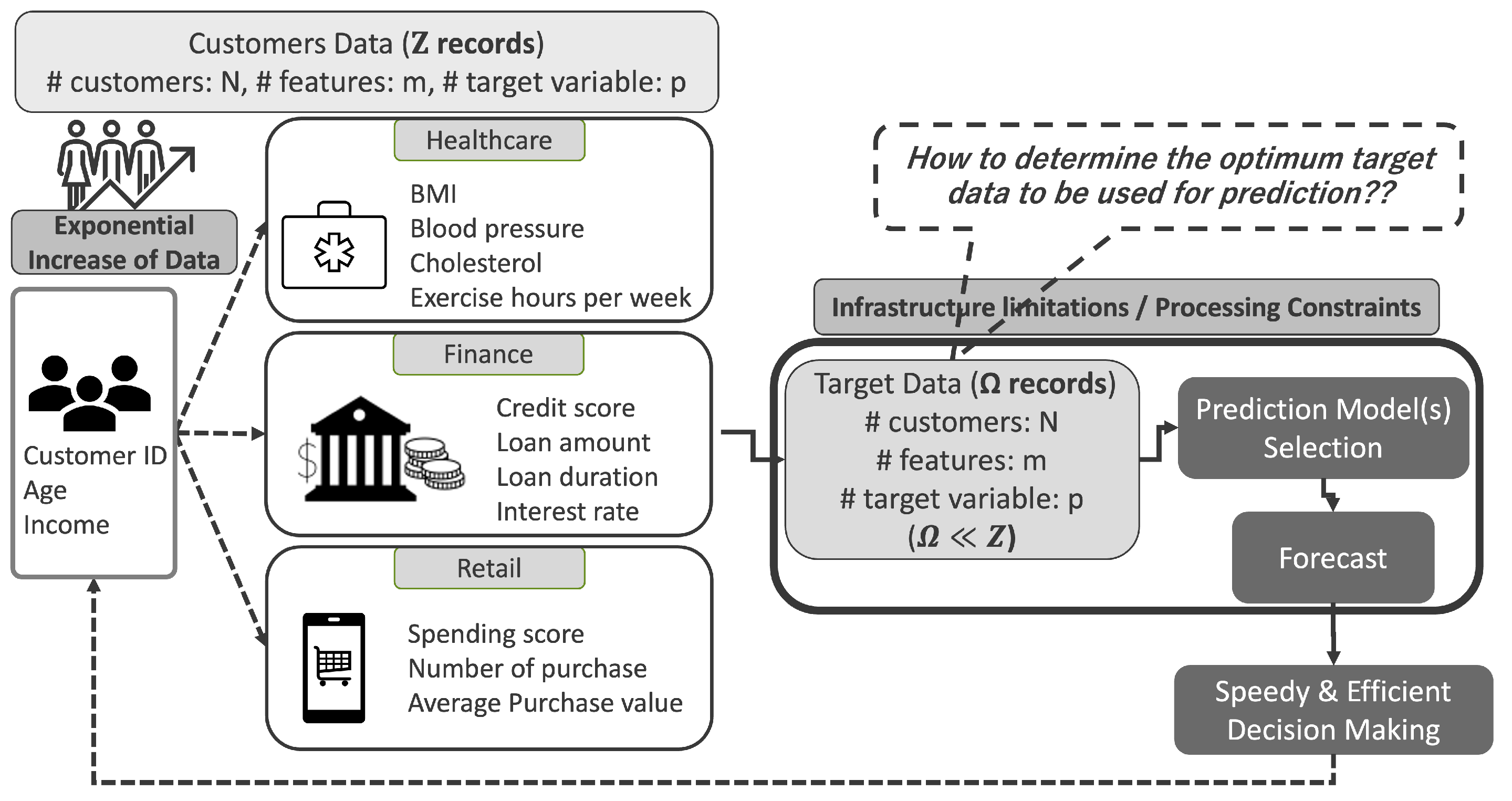
Figure 2.
Proposed Solution Architecture. (Phase 1 represents the scope of this paper while phase 2 represents the next phase of our proposal)
Figure 2.
Proposed Solution Architecture. (Phase 1 represents the scope of this paper while phase 2 represents the next phase of our proposal)
Figure 3.
Segmentation Based Proposal. (Given a dataset of size records, features, and targets, with a physical processing constraint of )
Figure 3.
Segmentation Based Proposal. (Given a dataset of size records, features, and targets, with a physical processing constraint of )
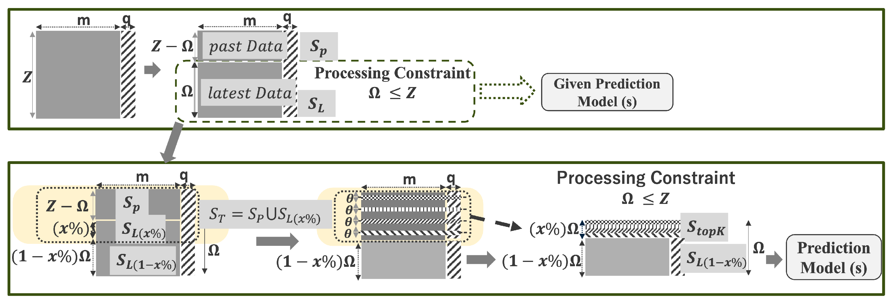
Figure 4.
Segmentation based Proposal Process Flow.
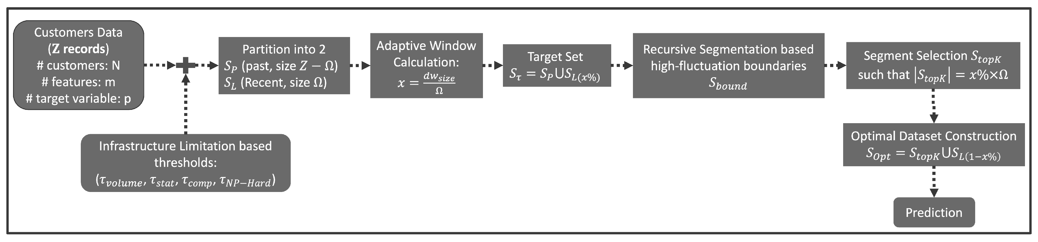
Figure 5.
Comparison of data selection strategies for the Bitcoin time series (2017-01-01 to 2021-02-28). (Top) The time series illustrating the ’No Segmentation’ baseline approach, which utilizes only the most recent data segment (red box) within the constraint. (Bottom) The time series showing the dynamically constructed optimal dataset using the Adaptive High-Fluctuation Recursive Segmentation (AHFRS) framework. This dataset is composed of the recent, statistically stable segment (black box) and the k=5 high-fluctuation historical segments (colored boxes) selected via likelihood-ratio-based recursive segmentation. These segments account for the dynamically computed of the training data.
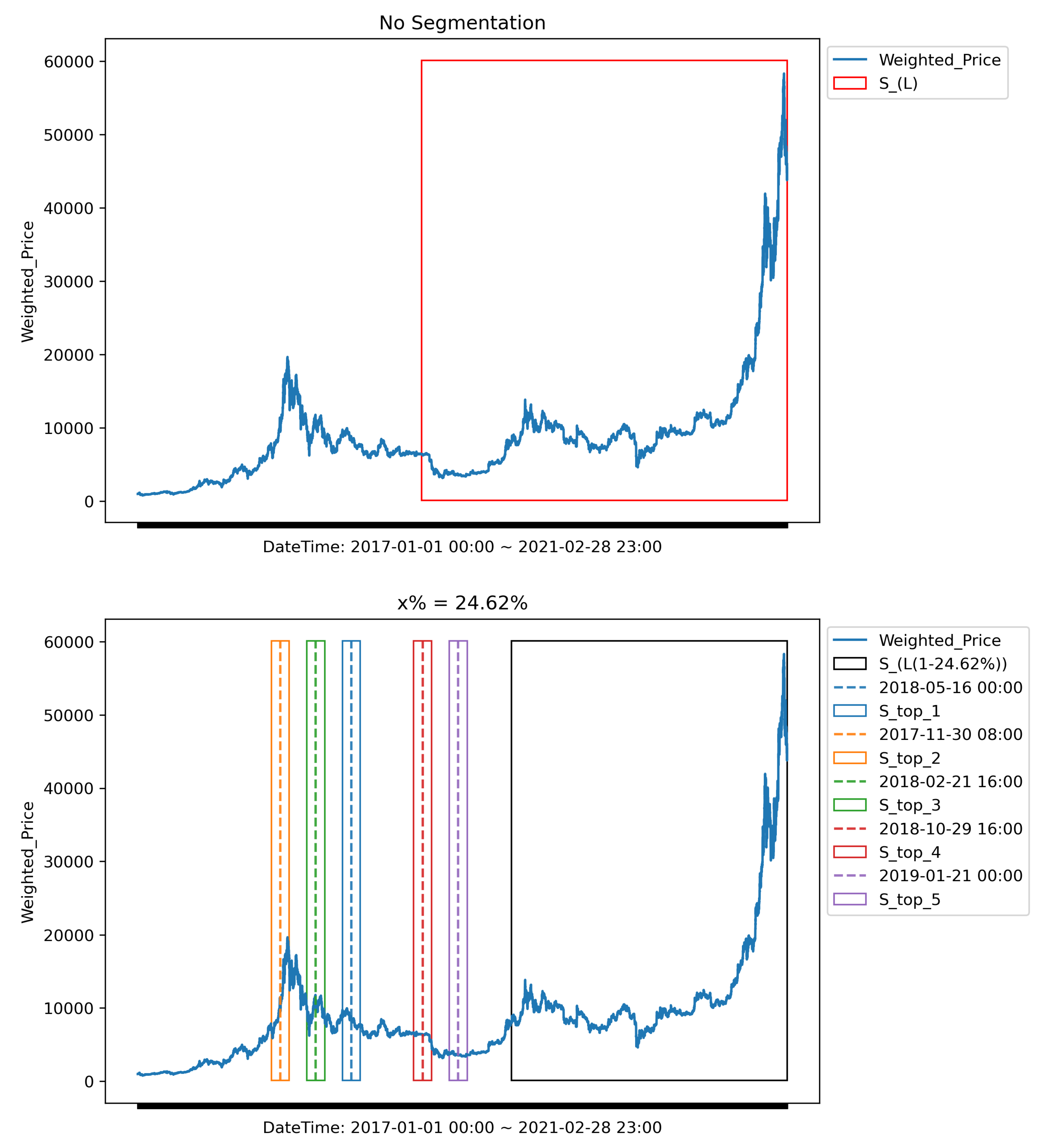
Figure 6.
Comparison of Actual and Predicted Bitcoin Weighted Prices for March 2021: Baseline vs. AHFRS-Enhanced Holt-Winters Forecasting.
Figure 6.
Comparison of Actual and Predicted Bitcoin Weighted Prices for March 2021: Baseline vs. AHFRS-Enhanced Holt-Winters Forecasting.
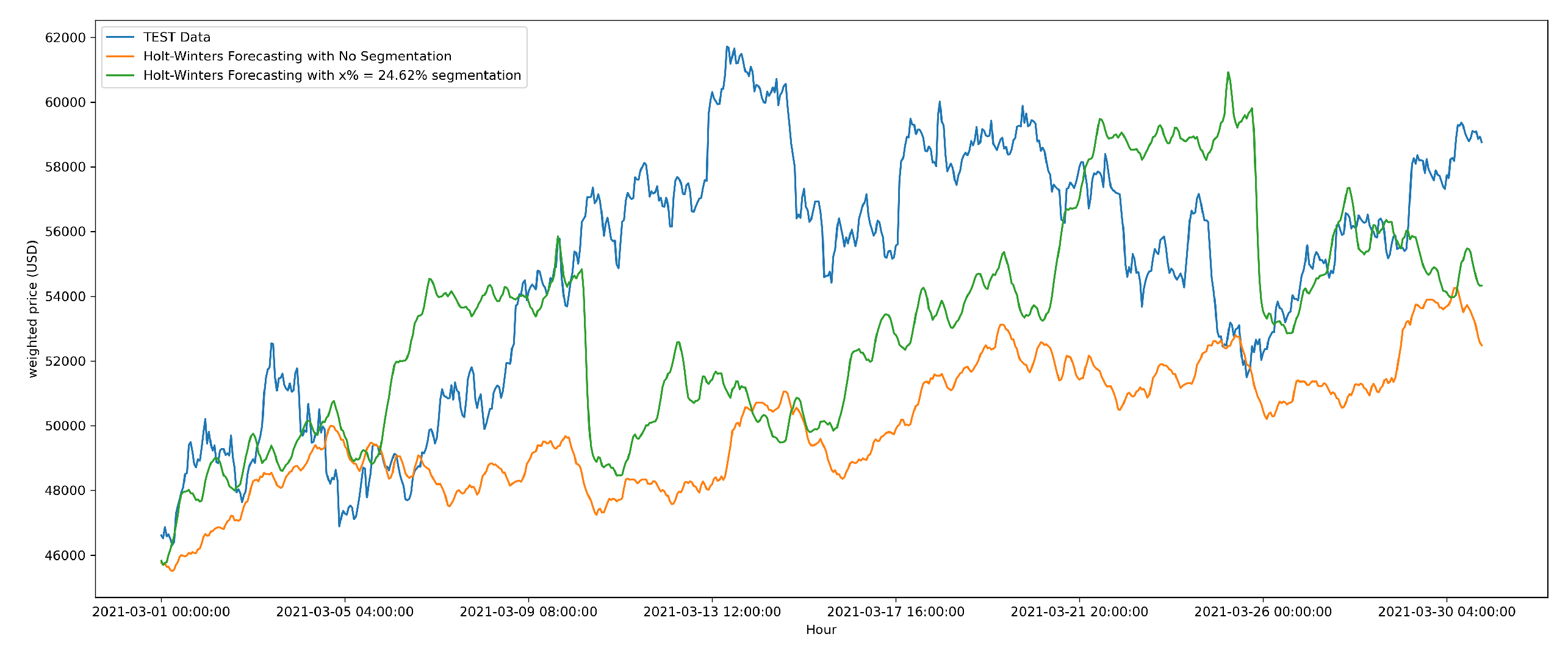
Figure 7.
Mean dynamic window size as a percentage of the constrained historical buffer across industries.
Figure 7.
Mean dynamic window size as a percentage of the constrained historical buffer across industries.
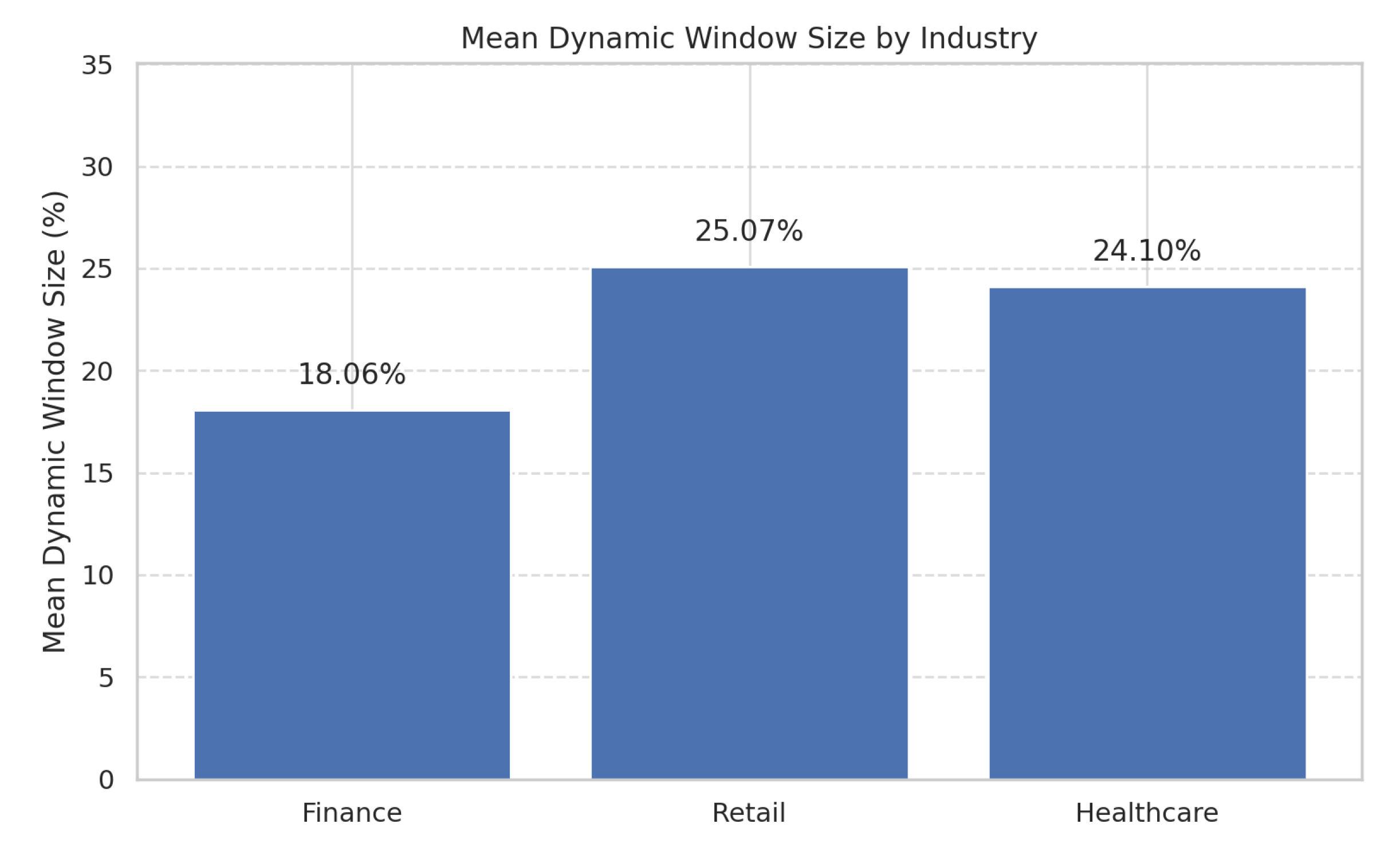

Table 1.
Comparison of some representative Statistical Complexity Measures.
| Measure | Purpose | Domain | Typical Use Case |
|---|---|---|---|
| López-Ruiz-Mancini-Calbet (CLMC) [33] | Balance between entropy and disequilibrium | Statistical physics | Identify intermediate complexity states |
| Excess Entropy [34] | Quantify mutual information across time | Dynamical systems | Memory and structure estimation |
| Statistical Complexity () [35] | Minimal memory for optimal prediction | Computational mechanics | Structural modeling |
| Kolmogorov Complexity (KC) [36,37] | Shortest description length / compressibility | Universal modeling | Algorithmic regularity, anomaly detection |
| Decision-Estimation Coefficient (DEC) [38] | Sample complexity of decision tasks | Interactive learning | Regret-bound estimation |
| Neural/Integrated Complexity () [39] | Causal integration and differentiation | Neuroscience, systems biology | Consciousness quantification |
Table 2.
Forecasting Performance of proposed AHFRS in comparison to Baseline.
| Dataset | Model | Scenario | RMSE | MAE | MAPE(%) |
|---|---|---|---|---|---|
| Hourly Bitcoin Weighted Price (USD) | Holt-Winters | Baseline | 5743.12 | 4916.20 | 8.69 |
| Proposal | 4517.31 | 3553.85 | 6.33 |
Table 3.
Forecasting Performance Comparison Across Industries and Models.
| Industry | Model | Scenario | Mean_RMSE | Mean_MAE | Mean_MAPE(%) |
|---|---|---|---|---|---|
| Finance | RF | Baseline | 0.72 | 0.58 | 21.79 |
| Proposal | 0.27 | 0.21 | 8.05 | ||
| GB | Baseline | 0.70 | 0.56 | 21.20 | |
| Proposal | 0.55 | 0.44 | 16.80 | ||
| Retail | RF | Baseline | 0.03 | 0.03 | 18.34 |
| Proposal | 0.01 | 0.01 | 6.84 | ||
| GB | Baseline | 0.03 | 0.03 | 17.94 | |
| Proposal | 0.02 | 0.02 | 14.47 | ||
| Healthcare | RF | Baseline | 4.48 | 3.59 | 15.83 |
| Proposal | 1.70 | 1.35 | 5.96 | ||
| GB | Baseline | 4.25 | 3.42 | 15.16 | |
| Proposal | 3.41 | 2.73 | 12.05 |
Disclaimer/Publisher’s Note: The statements, opinions and data contained in all publications are solely those of the individual author(s) and contributor(s) and not of MDPI and/or the editor(s). MDPI and/or the editor(s) disclaim responsibility for any injury to people or property resulting from any ideas, methods, instructions or products referred to in the content. |
© 2025 by the authors. Licensee MDPI, Basel, Switzerland. This article is an open access article distributed under the terms and conditions of the Creative Commons Attribution (CC BY) license (https://creativecommons.org/licenses/by/4.0/).
Copyright: This open access article is published under a Creative Commons CC BY 4.0 license, which permit the free download, distribution, and reuse, provided that the author and preprint are cited in any reuse.


