
Submitted:
31 January 2025
Posted:
03 February 2025
You are already at the latest version
Abstract
Accurate retail demand forecasting is essential for optimizing operations, improving customer satisfaction, and enhancing financial performance. Traditional statistical models often struggle to handle the complexities of retail time series data, which include hierarchical structures, irregular patterns, and external influencing factors. In this study, we evaluate the effectiveness of various Transformer-based models for probabilistic time series forecasting in retail, leveraging the rich explanatory variables provided by the M5 dataset. The models incorporate diverse features, including calendar-related information, selling prices, and socio-economic indicators such as SNAP activities, to capture the temporal, promotional, and socio-economic dynamics influencing sales. Our results demonstrate that Transformer-based models augmented with explanatory variables outperform their counterparts, providing more accurate and reliable forecasts across different horizons. We show that these models can effectively leverage context to improve forecast accuracy and capture uncertainty through probabilistic forecasting methods. This study highlights the potential of deep learning models in retail demand forecasting and underscores the importance of integrating domain-specific variables to achieve robust, context-aware predictions in dynamic retail environments.
Keywords:
Transformers
; time series
; probabilistic forecasting
; retail
; covariates
; deep learning
; data-driven decision-making
1. Introduction
Accurate forecasting models are fundamental to the retail industry, as they play a pivotal role in optimizing operations, enhancing customer satisfaction, and improving financial performance [1]. Retail businesses operate in a complex environment influenced by dynamic consumer behavior, seasonal trends, promotional activities, and external factors such as economic conditions and weather. As a result, the ability to anticipate demand accurately is essential for effective decision-making at strategic, tactical, and operational levels [2].
At the strategic level, forecasting models inform long-term decisions such as market entry strategies, channel development, and store location planning. These decisions require robust aggregate sales forecasts to understand market trends and the potential impacts of technological advancements or competitive shifts. For example, accurate forecasts enable retailers to decide whether to expand into online channels or develop smaller, local stores in response to evolving consumer preferences.
Tactically, forecasts guide mid-term planning, such as promotional strategies, category management, and inventory allocation. Retailers use these models to determine optimal pricing, promotional frequencies, and assortments that maximize profitability while minimizing waste. Accurate forecasts also ensure product availability during peak demand periods, maintaining high service levels and strengthening customer loyalty.
Operationally, accurate forecasts address immediate needs such as store-level inventory management, workforce scheduling, and replenishment planning. These tasks require high-granularity data, often at the stock-keeping unit (SKU) level, to minimize stockouts and overstocking [3]. For instance, ensuring sufficient inventory levels during a promotional campaign avoids missed sales opportunities while preventing excess stock that can lead to markdowns or spoilage. Moreover, the financial implications of inaccurate forecasting are significant. Retail operates on thin margins, where misaligned inventory levels can lead to substantial losses. Overestimations result in higher storage costs and markdowns, while underestimations lead to lost sales and customer dissatisfaction. Accurate forecasting models mitigate these risks, providing a balance between demand and supply, which is crucial for cash flow optimization and profitability.
Deep learning models have emerged as a superior approach to time series forecasting in retail, surpassing traditional statistical methods in handling the complexities and dynamic demands of this domain [4]. Statistical models such as ARIMA or exponential smoothing excel in forecasting tasks with straightforward trends and seasonality but often struggle when dealing with high-dimensional, hierarchical data structures, irregular sales patterns, and the integration of external influencing factors [5]. In contrast, deep learning models are capable of capturing intricate temporal patterns and dependencies across multiple time series [6,7]. Empirical evidence from the M4 competition and subsequent Kaggle competitions underscores the performance superiority of deep learning models in diverse scenarios [8]. For example, the Wikipedia Web Traffic competition demonstrated the ability of recurrent neural networks to outperform statistical benchmarks by effectively modeling long-term dependencies and incorporating contextual data. Similarly, the Corporación Favorita Grocery Sales competition showcased how ensembles of neural networks and gradient boosting methods excelled in scenarios involving hierarchical and disaggregated sales data. Another critical advantage of deep learning is its capacity for cross-learning, where patterns are learned across multiple time series [9]. This contrasts with traditional models that often require separate parameter estimation for each time series. Cross-learning enables deep learning models to generalize better and produce more robust forecasts, particularly in cases of sparse or noisy data. The findings of the M5 competition underscore this advantage [10]. The competition utilized large-scale, hierarchical sales data from Walmart, requiring forecasts across multiple aggregation levels and incorporating external variables like pricing and special events. Deep learning models, especially when combined with ensemble methods, demonstrated their capacity to outperform statistical benchmarks by effectively integrating external factors and exploiting the hierarchical structure of the data [11]. Additionally, deep learning methods provide probabilistic forecasts, allowing for the estimation of uncertainty and prediction intervals, a critical aspect in retail decision-making for inventory management and promotional planning. These capabilities enable retailers to align supply with demand more effectively, reduce costs from overstocking, and mitigate risks of stockouts [12].
The Transformer architecture has revolutionized deep learning, particularly in applications requiring efficient handling of sequential data. While traditional neural networks and Recurrent Neural Networks (RNNs) were pivotal in earlier stages of sequence modeling, they face specific limitations that restrict their effectiveness in capturing complex dependencies within sequences [13]. Traditional neural networks, for instance, lack a mechanism to retain information across steps in a sequence, rendering them inadequate for tasks requiring an understanding of long-range dependencies. RNNs, designed to address this by incorporating recurrence, have their own limitations, notably the vanishing gradient problem, which severely hampers their ability to learn dependencies over long sequences. To alleviate the vanishing gradient issue, Long Short-Term Memory (LSTM) networks and Gated Recurrent Units (GRUs) were introduced, enhancing RNNs with memory cells that can preserve information over extended steps [14]. These architectures improved the ability of recurrent networks to model longer dependencies, but they still suffer from key drawbacks, especially in terms of processing speed and scalability. The sequential nature of RNNs, including LSTMs, prevents parallel processing, resulting in slow training times and increased computational costs, particularly when applied to large datasets. The Transformer architecture overcomes these limitations through its groundbreaking self-attention mechanism. Unlike RNNs, Transformers enable parallel processing of data, which allows them to analyze all elements in a sequence simultaneously, dramatically improving both speed and computational efficiency. Self-attention empowers Transformers to weigh the relevance of each element in relation to others, regardless of their position within the sequence, facilitating a comprehensive understanding of context. This enables the model to capture long-range dependencies without the constraints of sequential processing. By dynamically adjusting the importance of different elements, Transformers excel at tasks that require both a deep understanding of context and the ability to model intricate relationships across a sequence. The combination of self-attention, parallel processing, and the ability to handle arbitrarily long dependencies has positioned Transformers as the leading architecture for tasks in natural language processing, computer vision, speech recognition, and time-series forecasting [6].
This paper introduces a comprehensive approach to probabilistic time series forecasting in retail using Transformer-based deep learning models. The study highlights the integration of explanatory variables such as promotions, pricing, and socio-economic indicators, demonstrating their impact on improving forecast accuracy. The models presented in this research outperform traditional statistical approaches by capturing complex temporal dependencies and hierarchical relationships across multiple aggregation levels.
The key contributions of this paper include:
- Development of Transformer-Based Forecasting Models: The study explores various Transformer-based architectures tailored for retail demand forecasting, including Vanilla Transformer, Informer, Autoformer, ETSformer, NSTransformer, and Reformer. These models are evaluated on their ability to capture long-term dependencies, seasonality, and external factors affecting sales patterns.
- Incorporation of Explanatory Variables: The research emphasizes the importance of integrating explanatory variables such as calendar events, promotional activities, pricing, and socio-economic factors in improving forecast accuracy. The models effectively leverage these covariates to address the complexities of retail data.
- Probabilistic Forecasting: The models provide probabilistic forecasts, capturing the uncertainty associated with demand predictions. This feature is crucial for risk management and decision-making processes in retail operations, ensuring a more resilient inventory management strategy.
- Empirical Evaluation Using Real-World Data: The paper includes a thorough empirical evaluation using the M5 dataset, a comprehensive retail dataset provided by Walmart. The results demonstrate the robustness and effectiveness of the proposed models in improving forecast accuracy across various retail scenarios.
The remainder of this paper is structured as follows. Section 2 provides a comprehensive review of recent advancements in retail time series forecasting, highlighting the evolution of deep learning models and the integration of explanatory variables. Section 3 describes the Transformer architectures used in this study and their application to probabilistic time series forecasting. Section 4 presents the dataset used, the experimental setup, and the results of the model evaluations, emphasizing the performance improvements achieved by the proposed approaches. Section 5 summarizes the key findings of the research, discusses the implications for retail operations, and suggests directions for future work.
This study aims to bridge the gap between advanced machine learning techniques and practical applications in the retail sector by demonstrating the potential of Transformer-based models to revolutionize demand forecasting. Through the integration of explanatory variables and probabilistic forecasting, the proposed models offer a comprehensive solution to the challenges of retail demand prediction, ultimately enhancing decision-making processes and operational efficiency.
2. Related Work
Recent advancements in retail time series forecasting have been driven by the growing capabilities of deep learning models, the strategic integration of explanatory variables, and the increasing emphasis on probabilistic methods to better capture uncertainties and dependencies, providing a comprehensive and nuanced approach to predicting consumer demand and optimizing inventory management [15].
2.1. Retail Time Series Forecasting with Deep Learning
The state-of-the-art in deep learning for time series forecasting in retail involves a range of innovative models and hybrid techniques to address the complexities of retail sales data [16]. Recent research has introduced diverse deep learning architectures designed to enhance the accuracy of sales forecasting in different retail contexts. Bandara et al. [17] present a demand forecasting framework for e-commerce using LSTM networks. By leveraging cross-series information from related products in a product hierarchy, the model provides accurate forecasts while addressing the challenges of non-stationary, sparse, and highly intermittent sales data. The proposed LSTM-based method significantly outperforms state-of-the-art univariate techniques, demonstrating its effectiveness for large-scale retail forecasting. Joseph et al. [18] proposed a hybrid deep learning framework combining Convolutional Neural Networks (CNN) with Bi-directional Long Short-Term Memory (BiLSTM) for store item demand forecasting. By utilizing CNN for feature extraction and BiLSTM for modeling temporal dependencies, the framework aims to enhance accuracy in predicting retail demand. Their approach, which employs Lazy Adam optimization, significantly outperforms traditional machine learning models, achieving lower forecasting errors and improving inventory decisions in the retail context. Giri and Chen [19] presented a deep learning framework for demand forecasting in the fashion and apparel retail industry. The proposed model combines image features of clothing items with sales data to predict weekly demand for new fashion products. The approach uses machine learning clustering to categorize products based on sales profiles and image similarity, resulting in accurate predictions even for newly launched items without extensive historical data. The study demonstrates the potential of integrating visual attributes and sales data to enhance forecast accuracy in fashion retail. Mogarala Guruvaya et al. [20] proposed a Bi-GRU-APSO model, which combines Bi-Directional Gated Recurrent Units (Bi-GRU) with Adaptive Particle Swarm Optimization (APSO) for retail sales forecasting. This hybrid approach uses feature selection techniques, including APSO, Recursive Feature Elimination (RFE), and Minimum Redundancy Maximum Relevance (MRMR), to enhance the accuracy and computational efficiency of forecasts. The model demonstrated superior performance on benchmark datasets, achieving higher accuracy metrics compared to conventional models, making it suitable for multi-channel retail sales forecasting. de Castro Moraes et al. [21] present a comparative analysis of deep learning models for optimizing single-period inventory decisions, focusing on the Newsvendor Problem. The study evaluates different deep learning architectures, including MLP, CNN, RNN, and LSTM, to determine their impact on inventory optimization by providing accurate demand forecasts. The results indicate that recurrent models, especially RNNs and LSTMs, outperform others in minimizing inventory mismatch costs. The research also shows that data-driven approaches that leverage empirical error distributions significantly outperform traditional model-based inventory methods. de Castro Moraes et al. [22] proposed hybrid deep learning models combining Convolutional Neural Networks with Long Short-Term Memory for retail sales forecasting. The study introduced stacked (S-CNN-LSTM) and parallel (P-CNN-LSTM) hybrid architectures to capture both temporal dependencies and external features in retail data. The models were evaluated using real-world retail datasets, outperforming simpler neural network architectures and standard autoregressive methods, while reducing computational complexity and improving both short-term and long-term forecasting accuracy. Additionally, Wu et al. [23] proposed a two-stage deep learning model called OCCPH-MHA for enhancing sales forecasting in multi-channel retail. The first stage uses a heterogeneous graph neural network to identify consumer group preferences based on purchase history, while the second stage integrates these preferences with time-series demand data using multi-head attention mechanisms. The model significantly improves sales forecast accuracy for multi-channel retail environments by leveraging consumer behavior insights and product preferences, showcasing its robustness in predicting demand across both online and offline channels. Finally, Sousa et al. [24] developed a two-stage model for predicting demand for new products in fashion retail using censored data. The first stage involved transforming historical sales data into demand using multiple heuristics and an Expectation-Maximization (EM) algorithm to estimate demand during stock-out events. The second stage used machine learning models—Random Forest, Deep Neural Networks, and Support Vector Regression—to predict demand for new products based on features of similar past items. The EM algorithm and Random Forest provided the most accurate predictions, demonstrating the model’s effectiveness in improving production management decisions for new product launches.
2.2. Explanatory Variables in Retail Demand Forecasting
The use of explanatory variables in retail time series forecasting has gained significant traction as researchers recognize the importance of incorporating external and contextual data to improve the accuracy of sales predictions. Various studies have highlighted how the integration of different external variables can enhance the performance of deep learning models in predicting retail sales. Huang et al. [25] explored the impact of competitive information, such as competitor prices and promotions, on forecasting sales of fast-moving consumer goods (FMCG) at the UPC level. The authors proposed a two-stage approach involving variable selection and factor analysis to effectively refine competitive explanatory variables, integrating them into an Autoregressive Distributed Lag (ADL) model. The study demonstrated that incorporating competitive information significantly improved forecasting accuracy compared to traditional methods, highlighting the importance of competitive dynamics in retail sales predictions. Loureiro et al. [26] explored the application of deep neural networks (DNN) for sales forecasting in the fashion retail industry. The study incorporated a wide set of explanatory variables, including physical product characteristics and domain expert opinions, to predict sales of new fashion products. The results showed that while the DNN performed well, its improvements over simpler methods, like Random Forest, were not always significant. The findings emphasize the importance of using both advanced modeling techniques and domain expertise to enhance sales predictions in fashion retail. Punia et al. [27] proposed a hybrid forecasting method combining Long Short-Term Memory networks and Random Forests (RF) for demand forecasting in multi-channel retail. The model leverages LSTM for temporal relationships and RF for handling explanatory variables, improving accuracy across both online and offline sales channels. Empirical evaluations show that the hybrid method outperforms other benchmark methods, demonstrating robustness in managing complex demand patterns across multiple channels in retail. Lim et al. [28] introduced the Temporal Fusion Transformer (TFT), an attention-based architecture for multi-horizon time series forecasting. TFT combines recurrent layers for local processing with self-attention layers to model long-term dependencies, enabling both high performance and interpretability. The model’s specialized components, such as gating mechanisms and variable selection networks, facilitate feature selection and enhance the relevance of temporal information. TFT demonstrated significant improvements in forecasting accuracy over benchmark models, making it suitable for retail and other applications that require reliable and interpretable multi-step predictions. Wang [29] proposed a novel framework that incorporates economic indicators and dynamic interactions to improve sales forecasting for different retail sectors, such as hypermarkets, supermarkets, and convenience stores. By identifying influential economic predictors like consumer price index (CPI), retail employment population (REP), and real wage, and by considering the competitive interactions between retail channels, the model enhances forecasting accuracy and provides managerial insights into sector-specific trends. The study demonstrates the potential of integrating macroeconomic indicators and inter-sector dynamics for optimized retail inventory and sales management. Kao and Chueh [30] presented a deep learning-based model for purchase forecasting aimed at reducing waste in food products with short shelf lives. The model uses Artificial Neural Networks (ANNs) to predict purchase quantities by incorporating factors such as store environment, weather, and consumer behavior. The proposed approach, tested on a cream puff product, effectively reduced forecasting errors with a mean-square percentage error (MSPE) of less than 6%. The study demonstrates the potential of integrating ANN-based forecasting into merchandising to enhance inventory efficiency and sustainability in retail operations. Ramos et al. [31] examined the use of shrinkage and dimensionality reduction techniques, specifically Ridge regression and Principal Component Analysis (PCA), for forecasting seasonal sales in retail. Their study focused on integrating multiple demand drivers, such as promotions and pricing, into statistical models like ARIMA and ETS. Empirical results using supermarket sales data showed that PCA-based models performed better during promotional periods, while shrinkage estimators outperformed alternatives during non-promotional periods, resulting in approximately 10% accuracy improvement over benchmark models. Punia and Shankar [32] proposed a deep learning-based decision support system for demand forecasting in retail, integrating sequence modeling with machine learning methods. The model effectively captures both temporal and covariate-based variations in demand data using structured and unstructured data sources, including promotions, weather, and economic indicators. The results demonstrated that the proposed ensemble model outperformed traditional statistical benchmarks, enhancing forecast accuracy and enabling more informed inventory and promotion planning for retailers. Nasseri et al. [33] conducted a comparative study on the application of tree-based ensemble models, specifically Extra Tree Regressors (ETRs), and Long Short-Term Memory networks for retail demand prediction. Utilizing a dataset of over 5.2 million records, including external factors like weather and COVID-19 data, the study found that ETR outperformed LSTM across multiple evaluation metrics, particularly in perishable product categories. This demonstrates the robustness of tree-based ensemble methods for capturing complex patterns in retail demand forecasting. Ramos and Oliveira [7] investigated the impact of incorporating static and dynamic covariates into deep learning models for sales forecasting. Using the DeepAR model, the study tested various combinations of time-, event-, price-, and ID-related features using the M5 competition dataset. Results indicated that incorporating time, event, and ID features significantly improved forecast accuracy, while price features offered minimal benefits. The optimal model achieved a 1.8% RMSSE (Root Mean Scaled Squared Error) and 6.5% MASE (Mean Absolute Scaled Error) improvement, emphasizing the value of feature integration for enhancing prediction reliability in retail forecasting. Wellens et al. [34] presented a simplified decision-tree framework for retail sales forecasting that effectively integrates explanatory variables. The study demonstrates that a streamlined implementation of tree-based machine learning methods, using variables such as promotions and national events, significantly outperforms traditional statistical models while maintaining computational efficiency. The framework’s success is largely attributed to the inclusion of feature engineering and explanatory variables, which improve forecast accuracy and reduce inventory costs, thereby making it more accessible for practical adoption by traditional retailers. Praveena and Prasanna Devi [35] proposed a hybrid deep learning model called Deep Prophet Memory Neural Network (DPMNN) for seasonal item demand forecasting in retail. By integrating temporal, historical, trend, and seasonal data, DPMNN outperformed state-of-the-art models such as LSTM and Prophet in reducing forecasting errors like RMSE and MAPE. The study demonstrates the efficacy of combining feature selection techniques with deep learning to optimize retail inventory management, effectively reducing overstock and stockouts.
2.3. Probabilistic Forecasting of Time Series Using Deep Learning
Probabilistic time series forecasting has gained prominence as an effective method for capturing uncertainty in predictions, providing valuable insights for decision-making across domains such as retail, finance, and supply chain management. Wen et al. [36] introduced the Multi-Horizon Quantile Recurrent Forecaster (MQ-RNN), a probabilistic forecasting framework that combines recurrent and convolutional neural networks with quantile regression for multi-step time series prediction. The model leverages both temporal and static covariates, effectively handling challenges like shifting seasonality, cold starts, and planned event spikes. By adopting a direct multi-horizon strategy, MQ-RNN mitigates error accumulation commonly found in recursive forecasting methods, providing stable and efficient performance, as demonstrated in applications for retail demand and energy forecasting. DeepAR, proposed by Salinas et al. [37], is another deep learning model that uses an autoregressive recurrent neural network to learn from related time series for probabilistic forecasting. By training on a large number of similar time series, DeepAR produces more accurate forecasts compared to traditional methods while effectively capturing the distribution of future values. This model uses an autoregressive framework that can integrate diverse data, providing flexibility for large-scale applications like retail demand prediction where individual time series are related through shared features such as product categories. Rasul et al. [38] introduced TimeGrad, an autoregressive denoising diffusion model for multivariate probabilistic time series forecasting. The model employs diffusion probabilistic methods, leveraging gradient estimation to generate accurate probabilistic forecasts for complex time series data with thousands of correlated dimensions. TimeGrad utilizes Langevin sampling to convert noise into samples of the distribution of interest. Experimental results demonstrated that TimeGrad sets a new state-of-the-art performance in multivariate probabilistic forecasting, outperforming existing methods across a range of real-world datasets. Rasul et al. [39] proposed a model for multivariate probabilistic time series forecasting using conditioned normalizing flows. The approach combines autoregressive deep learning techniques with normalizing flows to capture complex dependencies across time series, enabling accurate probabilistic predictions. The model achieves scalability while retaining high-dimensional dependency representation, making it suitable for scenarios involving thousands of interacting time series. Empirical evaluations on various real-world datasets demonstrated that this method outperformed existing baseline models in terms of accuracy and computational efficiency. Hasson et al. [40] introduced the Level Set Forecaster (LSF), a novel algorithm designed to transform any point estimator into a probabilistic forecaster. By leveraging the grouping of similar predictions into partitions, LSF creates consistent probabilistic forecasts, particularly when used with tree-based models like XGBoost. Empirical evaluations demonstrated that LSF rivals state-of-the-art deep learning models in forecasting accuracy, providing a significant advancement in turning point predictions into probabilistic forecasts effectively. Rangapuram et al. [41] proposed an end-to-end approach for generating coherent probabilistic forecasts for hierarchical time series. Unlike traditional two-step methods that require separate reconciliation processes, this model incorporates reconciliation as part of a single trainable framework, ensuring coherent predictions across all levels of a hierarchy. By leveraging the reparameterization trick and a differentiable convex optimization layer, the model is capable of simultaneously learning from all time series in a hierarchy while maintaining coherence without post-processing. Empirical results demonstrated significant improvements in forecast accuracy, making this approach highly effective for large-scale applications like retail and energy demand forecasting. Kan et al. [42] proposed the Multivariate Quantile Function Forecaster (MQF2), a probabilistic forecasting method designed to improve multi-horizon predictions by using a multivariate quantile function. MQF2 combines elements of autoregressive and sequence-to-sequence models to capture the dependency structure across time, thereby avoiding error accumulation and quantile crossing. The model is particularly effective in inventory management scenarios, enhancing forecasting accuracy for supply chain decisions by integrating dependencies like product cannibalization and substitutability. Shchur et al. [43] introduced AutoGluon–TimeSeries, an open-source AutoML library designed for probabilistic time series forecasting. The framework enables users to generate accurate point and quantile forecasts with minimal coding effort by leveraging ensembles of diverse forecasting models. AutoGluon–TimeSeries demonstrated strong empirical performance on 29 benchmark datasets, outperforming existing methods in terms of both point and probabilistic forecast accuracy, making it a robust solution for practitioners with varying levels of expertise. Tong et al. [44] introduced a hierarchical Transformer model with probabilistic decomposition, called Probabilistic Decomposition Transformer (PDTrans), designed to mitigate the cumulative errors common in autoregressive forecasting. By combining a Transformer for primary autoregressive forecasting with a conditional generative model, PDTrans enables hierarchical, probabilistic, and interpretable forecasts. The model effectively separates seasonal and trend components, providing accurate forecasts for complex temporal patterns, as demonstrated across multiple time series datasets. Sprangers et al. [45] introduced a bidirectional temporal convolutional network (BiTCN) for probabilistic time series forecasting, focusing on reducing the parameter count required by traditional Transformer-based methods. The model uses two temporal convolutional networks to encode future covariates and past observations, respectively, enabling efficient and accurate forecasting. The study demonstrated that BiTCN performs on par with state-of-the-art methods while requiring fewer parameters, significantly reducing both memory usage and training costs, thus making it a more accessible option for large-scale forecasting tasks. Lastly, Olivares et al. [46] introduced the Deep Poisson Mixture Network (DPMN) for probabilistic hierarchical forecasting. The model combines neural networks with a mixture of Poisson distributions to produce coherent forecasts at different aggregation levels without requiring explicit reconciliation steps. DPMN ensures hierarchical coherence, making it particularly effective for large-scale forecasting tasks. Empirical evaluations demonstrated significant improvements over existing methods, achieving an 11.8% better CRPS score on Australian tourism data and an 8.1% improvement on grocery sales data.
3. Probabilistic Forecasting with Transformer-based Models
The Transformer architecture’s reliance on attention mechanisms, rather than recurrence, allows for significant parallelization, which reduces training time while maintaining high performance. The use of self-attention throughout the encoder and decoder stacks enables the model to effectively capture long-range dependencies in the data, making it especially powerful for tasks that involve complex sequential relationships. In time series forecasting, sequences of numerical observations are treated similarly to sequences of words or tokens in language models, as both require understanding and capturing dependencies across ordered elements. This analogy is reflected in the application of Transformer-based architectures, as introduced by Vaswani et al. [47], which were originally developed for natural language processing but have proven highly effective for time series tasks [28], where learning complex temporal patterns is akin to learning relationships between words in a sentence. In the following section, we present the Vanilla Transformer [47], Informer [48], Autoformer [49], ETSformer [50], NSTransformer [51], and Reformer [52] architectures. These models were chosen for their availability [53], widespread use [54], and demonstrated effectiveness in performance assessment [15], providing a balanced comparison between well-established approaches and recent advancements tailored specifically for time series forecasting. These architectures were also employed in the empirical study conducted for this paper.
3.1. Deep Learning Transformers for Time Series Forecasting
Vaswani et al. [47] introduced the Transformer architecture, which revolutionized the field of deep learning by relying entirely on attention mechanisms rather than traditional recurrent or convolutional layers for sequence transduction tasks. The architecture is composed of an encoder-decoder structure, where both the encoder and decoder are built using multiple identical layers stacked on top of each other. The encoder comprises identical layers, each of which includes a multi-head self-attention mechanism and a position-wise feed-forward network. Each layer uses residual connections followed by layer normalization, allowing the model to retain information and stabilize training. The attention mechanism enables the encoder to capture dependencies between all elements in the input sequence, regardless of their relative positions. The decoder also consists of identical layers, but with an additional sub-layer compared to the encoder. In each decoder layer, multi-head self-attention is combined with encoder-decoder attention, allowing the decoder to attend to the output of the encoder stack. Additionally, a masking mechanism is applied to prevent positions from attending to subsequent positions, ensuring that the model maintains its autoregressive properties. Attention mechanisms are the core of the Transformer architecture, enabling it to effectively weigh the relevance of different parts of the input sequence.
The computation of attention relies on three main components: queries (), keys (), and values (). To derive these components, the input matrix is multiplied by learnable weight matrices for queries, keys, and values, yielding , , and :
Using these matrices, the attention mechanism computes query-key interactions by multiplying with the transpose of , applying a scaling factor, followed by a softmax activation, and finally multiplying with . This results in a matrix of size . To address numerical instability and prevent the vanishing gradient problem during training, the dot product is scaled by dividing by the square root of the key dimension . The final output of self-attention, where each row corresponds to the output vector for a given query, is computed as follows:
Multi-Head Attention uses multiple sets of learned projections to perform attention in parallel, allowing the model to attend to different subspaces of the input information simultaneously. To handle the sequential nature of data, the model also incorporates positional encodings that provide information about the relative positions of elements in the sequence. This is crucial as the architecture lacks any recurrence or convolution, making it necessary to add position information explicitly to allow the model to understand the order of the sequence. Figure 1 provides a detailed depiction of this architecture along with the others discussed in this section, highlighting the specific components and attention mechanisms that characterize each Transformer variant.
In their work, Zhou et al. [48] introduce a new Transformer-based architecture designed specifically for the challenges of long sequence time-series forecasting (LSTF). The architecture, named Informer, focuses on improving computational efficiency and scalability for long input sequences, addressing the limitations of traditional Transformer models like high computational complexity and memory usage. The Informer architecture follows an encoder-decoder framework but with several key innovations. The encoder uses the ProbSparse self-attention mechanism, which replaces the canonical dot-product self-attention with a probabilistic sampling approach. This allows Informer to achieve a time complexity and memory usage of , significantly reducing the quadratic complexity typically seen in standard Transformer architectures, making it suitable for long sequence data. Additionally, self-attention distilling is applied within the encoder to highlight dominant attention scores and reduce redundant input combinations. This operation significantly compresses the attention map, reducing the space complexity while still preserving important information. The encoder outputs a refined representation that maintains robust long-range dependencies. The decoder employs a generative style that predicts the entire output sequence in a single forward pass rather than the traditional step-by-step dynamic decoding. This drastically improves the inference speed, particularly for long sequences, and prevents the accumulation of errors that is common in autoregressive decoding. The combination of ProbSparse attention, self-attention distilling, and the generative decoder makes Informer an efficient and scalable solution for long-term forecasting. The Informer model has demonstrated superior performance in capturing long-range dependencies while being computationally feasible for very large datasets, making it highly suitable for empirical studies involving long sequence time-series forecasting in various domains, such as finance and energy.
Wu et al. [49] propose a novel architecture specifically designed to improve long-term time series forecasting, called Autoformer. This model innovates by moving beyond the limitations of the canonical Transformer, particularly addressing the inefficiencies associated with traditional self-attention mechanisms in long-term forecasting contexts. The Autoformer architecture follows an encoder-decoder framework but diverges from the typical self-attention approach by incorporating series decomposition blocks and an Auto-Correlation mechanism. The encoder is designed to eliminate the trend-cyclical components using series decomposition blocks, which allows it to focus on modeling seasonal patterns effectively. Each encoder layer includes a series decomposition operation, which progressively separates the seasonal and trend components, making the hidden representations more suitable for accurate long-term forecasting. In the decoder, Autoformer includes an accumulation mechanism for trend components and stacked Auto-Correlation blocks for refining seasonal components. The unique Auto-Correlation mechanism replaces self-attention to discover dependencies based on series periodicity and to aggregate similar sub-series, thus enhancing both computational efficiency and the utilization of information from the entire sequence. This mechanism reduces the computational complexity from the quadratic order (as seen in Vanilla Transformers) to , making it feasible for long-term sequences. The combination of progressive decomposition and Auto-Correlation mechanisms allows Autoformer to handle intricate temporal patterns more effectively while maintaining computational efficiency. Empirical evaluations have shown that Autoformer achieves state-of-the-art results across multiple benchmarks in applications such as energy, traffic, economics, weather, and disease forecasting.
Woo et al. [50] present a novel transformer architecture tailored for time-series forecasting by combining traditional exponential smoothing concepts with the Transformer framework. The model, named ETSformer, is specifically designed to enhance long-term time series prediction while maintaining interpretability and computational efficiency. The ETSformer architecture builds on an encoder-decoder design that incorporates Exponential Smoothing Attention (ESA) and Frequency Attention (FA) mechanisms to address the limitations of the Vanilla self-attention used in standard transformers. The architecture consists of modular decomposition blocks that extract time-series components like level, growth, and seasonality at each layer, effectively breaking down complex time series into interpretable sub-components. The encoder is responsible for decomposing the time series data into latent seasonal and growth representations, while the decoder combines these components to produce the final forecast. Exponential Smoothing Attention replaces the traditional dot-product attention mechanism with an attention function that emphasizes recent observations, similar to the exponential smoothing method commonly used in traditional forecasting models. This approach enhances the model’s ability to predict trends over time. Frequency Attention, on the other hand, uses Fourier transformation to identify and extract dominating seasonal patterns, which allows the model to effectively capture recurring behaviors. The combination of Exponential Smoothing and Frequency Attention ensures that the model not only achieves a state-of-the-art performance in terms of forecasting accuracy but also maintains interpretability by explicitly modeling level, growth, and seasonal components. The ETSformer was empirically evaluated on multiple benchmark datasets and showed significant improvements over existing Transformer-based approaches for time series forecasting.
NSTransformer, introduced by Liu et al. [51] was designed to overcome the limitations of traditional Transformers in handling non-stationary time series data. This model combines two core components: Series Stationarization and De-stationary Attention, which together enable effective modeling of non-stationary real-world data. The NSTransformer architecture follows a standard Transformer encoder-decoder structure but introduces innovations specifically for handling non-stationary data. The Series Stationarization module applies a normalization technique that unifies key statistics (mean and variance) of each input time series, thereby stabilizing the input distribution for better generalization. This module acts as a preprocessing step that makes non-stationary inputs more tractable for the Transformer. However, to address the problem of over-stationarization (where stationarization causes loss of valuable temporal characteristics of the original data), NSTransformer also includes a De-stationary Attention mechanism. This attention mechanism restores the original non-stationary properties that were lost during stationarization. By using a learned de-stationary factor, this mechanism approximates the attention that would have been obtained from raw non-stationary data, ensuring that the model retains the distinct temporal dependencies necessary for accurate forecasting. The NSTransformer also incorporates a two-stage transformation process: normalization before feeding data to the model and de-normalization after generating outputs, which transforms predictions back to the original scale. These features make the NSTransformer suitable for effectively leveraging non-stationary information while maintaining the computational efficiency and long-term dependency capabilities of standard Transformer-based models.
Kitaev et al. [52] introduce the Reformer, an efficient Transformer architecture specifically designed to handle long sequences with reduced computational and memory requirements. The Reformer makes significant architectural changes to the original Transformer by incorporating Locality-Sensitive Hashing (LSH) Attention and Reversible Residual Layers. The LSH Attention mechanism is a key innovation of the Reformer. Traditional Transformers use scaled dot-product attention, which has a computational complexity of , where L is the sequence length, making it infeasible for long input sequences. Reformer replaces this with Locality-Sensitive Hashing to approximate attention, reducing the complexity to . In this approach, the keys and queries are hashed into buckets such that only similar elements are grouped together for attention calculations. This significantly reduces the number of dot products computed while still capturing the most important relationships between elements, making it possible to efficiently handle long sequences. The second major modification is the use of Reversible Residual Layers. In standard Transformer architectures, each layer requires storing intermediate activations for backpropagation, which scales linearly with the number of layers, creating a large memory burden. Reformer addresses this by employing reversible residual connections, inspired by RevNets, which allow activations from previous layers to be reconstructed during backpropagation, rather than stored. This approach effectively eliminates the need for storing layer-wise activations, significantly reducing memory usage during training. Additionally, chunking is applied to feed-forward layers to further manage memory usage. The feed-forward layers, typically responsible for large intermediate activations, are processed in smaller chunks, reducing the peak memory requirement without affecting the model’s performance. This enables Reformer to efficiently handle feed-forward computations for long sequences. The combination of LSH Attention, Reversible Residual Layers, and chunked feed-forward processing allows the Reformer to maintain the expressive power of the original Transformer architecture while being significantly more efficient in both memory and computation. The Reformer is particularly suitable for tasks involving long sequences, such as language modeling and time-series forecasting, where traditional Transformers face scalability issues.
3.2. Probabilistic Forecasting of Time Series Data
Let represent a dataset consisting of N univariate time series, where each uniformly-spaced time series contains observations, and denotes the value of the i-th time series at time t [43]. For example, might indicate the number of units sold of product i on day t. To simplify the notation, we will assume that all time series have the same length T, even though the models can handle time series of varying lengths. The goal of time series forecasting is to predict the next H values for each time series in , where H is referred to as the prediction length or forecast horizon. Additionally, each time series may have associated covariates , which can include both static and time-varying features. Static covariates are attributes that remain constant across time, such as store location or product ID. Time-varying covariates change over time and could include factors like the day of the month or planned promotions.
The problem of probabilistic time series forecasting can be formally described as modeling the joint conditional distribution of the future time series values , given its historical observations , and any associated covariates, . This is represented as [36]:
where denotes the parameters of the parametric distribution being modeled. Thus, the objective of probabilistic time series forecasting is not just to provide a single point prediction but to estimate the full conditional distribution, capturing the inherent uncertainty in the future values [55]. This allows for more robust decision-making in applications where the range of possible outcomes and their probabilities are as critical as the predictions themselves.
In practice, instead of using the entire history of each time series i, which can vary significantly, we can focus on extracting fixed context windows of size [56]. This approach involves sampling subsequences from the full time series, allowing us to estimate the conditional distribution of the next H future values based on the selected context window and the corresponding covariates. This conditional distribution can be expressed as:
It is worth noting that the initial time step of the context window does not necessarily align with the beginning of the time series. When a neural network with weights is used to model this distribution, predictions are conditioned on these learned parameters. To estimate the conditional distribution described above, inspired by Rasul et al. [38], Rasul et al. [39], an autoregressive approach can be applied, leveraging the chain rule of probability as follows:
The tokenization process employed in this study involves creating lagged features based on past values of the time series, tailored to align the data’s frequency [56]. Based on the recommendations of Alexandrov et al. [57], we selected appropriate lag values for various frequencies, including quarterly, monthly, weekly, daily, and hourly. For a given frequency, a sorted set of positive lag indices, , is defined, where represents the largest lag index in the set. These lag indices are generally not evenly spaced in time. Lag features are then generated for each context window . This process involves sampling from an extended window containing additional historical points, denoted as [56]. If a total of K static and dynamic covariates are added to these lagged features, the resulting token for each time series value will have a size of Figure 2 illustrates this tokenization process.
As shown in Figure 2, the architecture of the probabilistic transformer-based models employed in this study consists of two main components: an encoder and a decoder. For the encoder, a sequence of C tokens is generated by tokenizing the data through the concatenation of covariates with lagged features sampled from the extended window . Similarly, for the decoder, the sequence of H tokens is created by concatenating covariates with lagged features sampled from the extended window Both encoder and decoder tokens are used during training. These tokens are then passed through a shared linear projection layer, which maps the features into the hidden dimension of the attention mechanism. To encode the position of each token in the sequence, positional encoding, as outlined by Vaswani et al. [47], is applied. This encoding uses a combination of sine and cosine functions at different frequencies, which are added to the token embeddings. By incorporating information about both relative and absolute positions, positional encoding allows the attention mechanism to effectively capture the sequential order of tokens, a critical aspect for time series modeling.
After processing data through the masked decoder layers, the model predicts the parameters for the forecast distribution of the next time step. These parameters are computed by a parametric distribution head, which serves as the model’s final layer. The distribution head projects the features learned by the model to the parameters of the selected probability distribution [56]. Various parametric distributions can be employed; in our experiments, we utilize the Student’s t-distribution, which outputs three parameters: mean , scale , and degrees of freedom . Training is performed by minimizing the negative log-likelihood of the forecasted distribution across all predicted time steps.
During inference, for a time series containing at least observations, a feature vector is tokenized and passed into the model to estimate the distribution of the subsequent time step. Using greedy autoregressive decoding, the model can simulate multiple future trajectories up to the defined forecast horizon . These simulations enable the computation of uncertainty intervals, which are critical for decision-making and for assessing the model’s accuracy on unseen data.
This methodology to probabilistic time series forecasting has been applied to the previously described transformer-based architectures, including the Vanilla Transformer [47], Informer [48], Autoformer [49], ETSformer [50], NSTransformer [51], and Reformer [52]. The implementation builds upon the tools and frameworks introduced by Kashif Rasul [53,58].
4. Empirical Evaluation
4.1. Dataset
The M5 dataset represents a significant advancement in the realm of retail forecasting by leveraging a publicly available dataset to facilitate transparent, reproducible, and rigorous evaluation of forecasting methodologies [59]. Publicly accessible datasets like the M5 are crucial for advancing the field as they enable researchers and practitioners to benchmark methods, validate results, and push the boundaries of innovation. This open access fosters collaboration, promotes replication of results, and provides a shared foundation for addressing complex forecasting challenges.
The M5 dataset, generously provided by Walmart, consists of 3,049 individual product time series of daily unit sales data spanning approximately 5.4 years, from January 29, 2011, through June 19, 2016, resulting in a total of 1,969 daily data points. The dataset includes products from three categories—Hobbies, Foods, and Household—sold across 10 stores located in three U.S. states: California, Texas, and Wisconsin. This hierarchical structure enables evaluations at multiple aggregation levels, ranging from total sales across all stores to individual product sales at specific locations, thereby reflecting the intricate, hierarchical, and multivariate nature of retail forecasting. The dataset’s comprehensive design ensures representation of diverse shopping behaviors, regional market dynamics, and product-specific trends, making it a robust resource for developing, benchmarking, and testing advanced forecasting models.
In this work, data from three stores—one from each state—were analyzed, resulting in a total of 9,147 distinct time series. This selection was made to accommodate limited computational resources for training the models while enabling a focused analysis that still represents the diversity and complexity of the dataset, capturing variations across regions, product categories, and store-level dynamics.
We adopted the framework of the M5 competition, reserving the final 28 days of each time series (from May 23, 2016, to June 19, 2016) as the testing set for out-of-sample evaluation. The earlier data, covering up to January 29, 2011, through May 22, 2016, was used to train the models.
4.2. Explanatory Variables
The M5 dataset includes several explanatory variables that enhance its utility for improving the accuracy of forecasting models in retail settings. These variables supplement the core sales data and enable the modeling of external factors influencing demand. The key exogenous variables in the M5 dataset are:
- Calendar-Related Information: This includes a wide range of time-related variables such as the date, weekday, week number, month, and year. Additionally, it includes indicators for special days and holidays (e.g., Super Bowl, Valentine’s Day, Orthodox Easter), which are categorized into four classes: Sporting, Cultural, National, and Religious. Special days account for about 8% of the dataset, with their distribution across the classes being 11% Sporting, 23% Cultural, 32% National, and 34% Religious.
- Selling Prices: Prices are provided at a weekly level for each store. The weekly average prices reflect consistent pricing across the seven days of a week. If a price is unavailable for a given week, it indicates that the product was not sold during that period. Over time, the selling prices may vary, offering critical information for understanding price elasticity and its impact on sales.
- SNAP Activities: The dataset includes a binary indicator for Supplemental Nutrition Assistance Program (SNAP) activities. These activities denote whether a store allowed purchases using SNAP benefits on a particular date. This variable accounts for about 33% of the days in the dataset and reflects the socio-economic factors affecting consumer purchasing behavior.
These variables are instrumental in enriching the dataset’s predictive power by providing critical contextual information. Calendar-related variables capture temporal effects such as seasonality and special events, helping models identify recurring patterns in consumer behavior. Price and promotional data offer valuable insights into how market conditions influence purchasing decisions, improving the model’s ability to forecast demand fluctuations. Additionally, socio-economic factors are well-represented through the inclusion of SNAP activities. The SNAP indicators reflect variations in demand driven by government assistance programs, which can significantly influence consumer spending behavior and sales dynamics. This is particularly relevant in economically vulnerable regions, where such programs play a key role in shaping purchasing patterns. By incorporating these diverse exogenous variables, the M5 dataset provides a robust foundation for developing sophisticated forecasting models that can effectively address the complexities of retail sales.
Table 1 presents a comprehensive summary of the input features (lags and covariates) used in the time series forecasting models. The table highlights the diversity of features extracted from the dataset to improve the models’ predictive accuracy.
The Sales feature includes 30 specific lag values representing historical sales observations used as inputs for forecasting. These lag values cover different time intervals to capture both short-term and long-term patterns, including daily, weekly, and annual cycles, ensuring the models have a broad temporal context. Several time-related features are included as categorical variables, such as Day of week, Day of month, Day of year, Month of year, Week of year, Week of month, and Year. These categorical time features, encoded as zero-based index and normalized to a range of [-0.5, 0.5], help the models account for seasonality and calendar effects. The Is weekend feature is a binary indicator used to identify weekends, which can impact sales patterns due to changes in consumer behavior. Another continuous feature included is Age, which represents the age of the product in the dataset. This is calculated as a logarithmic transformation of the number of sale days and helps capture the effect of product lifecycle on sales. The table also includes three price-related features, representing the daily price of items normalized by different factors: the mean and standard deviation of item prices, department prices, and store prices. These features capture the impact of price changes on sales. SNAP activities are included as a categorical feature indicating whether purchases were allowed using the Supplemental Nutrition Assistance Program (SNAP) benefits in the states of California, Texas, and Wisconsin. This variable captures socio-economic factors that influence consumer demand. The Events feature accounts for 31 distinct special days, such as holidays and other significant events, categorized into four classes: Sporting, Cultural, National, and Religious. Including these variables helps the models account for spikes or drops in sales associated with specific events. Additionally, ID features are included to capture hierarchical information from the dataset. These IDs include item IDs, department IDs, category IDs, store IDs, and state IDs, each encoded as categorical variables. The IDs are embedded using a learnable embedding layer to help the model understand relationships across different levels of the hierarchy, such as items within a department or stores within a state.
4.3. Hyperparameter Tuning
Selecting a model that performs consistently well in out-of-sample predictions is a crucial step in the modeling process. To achieve this, it is common practice to use a validation set for distinguishing between competing models. Considering that deep learning models can be sensitive to hyperparameter settings and initialization, an effective strategy for model selection becomes essential. In this study, the final 28 days of the training period, from April 25 to May 22, 2016, were designated as a validation set to objectively compare and rank different model configurations.
To explore the hyperparameter space systematically and identify optimal settings, this study employed the Optuna framework [60], an advanced tool for hyperparameter optimization. Optuna is an open-source Python library designed to streamline the process of hyperparameter tuning, particularly for machine learning models, including those based on Transformers. The framework offers dynamic search space construction through its define-by-run API and supports efficient search strategies like Tree-structured Parzen Estimator (TPE), Random Search, and Grid Search. Additionally, Optuna includes pruning techniques to optimize computational resources and integrates seamlessly with popular machine learning frameworks such as PyTorch. The optimization process in Optuna involves defining an objective function, conducting a study, running the optimization trials, and analyzing the resulting configurations. This approach simplifies the time-consuming task of tuning hyperparameters, allowing researchers to focus more on refining their models and interpreting results. By employing this robust optimization tool, the study ensured that the selected hyperparameter configurations enhanced the performance and reliability of the forecasting models.
Table 2 outlines the hyperparameter search spaces explored in this study using the Optuna hyperparameter optimization (HPO) framework. Optuna was employed to randomly sample values from these predefined spaces, generating a variety of model configurations. The configuration that achieved the highest validation score, based on the Mean Weighted Quantile Loss (MWQL), was selected as the optimal model. MWQL, a metric specifically designed for evaluating probabilistic forecasts, which approximates (a weighted average of) the continuous ranked probability score (CRPS) [61], provides a comprehensive assessment of accuracy across multiple quantile levels, making it an effective criterion for ranking model performance, as defined in Equation (8). The table details the ranges of key hyperparameters, including context length, batch size, and the number of encoder and decoder layers used across the evaluated Transformer-based models. The context length, ranging from 28 days to multiples of 28-day periods, defines the historical time window used in training, with different lengths aiming to capture a range of temporal patterns from short-term fluctuations to more extended seasonal trends. The batch size parameter varies between 32 and 256, impacting the number of data samples processed in one iteration, thus affecting training stability and efficiency. Furthermore, the number of encoder and decoder layers represents the model’s depth. Deeper models, such as those with up to 16 encoder layers, are capable of learning more complex patterns, but they also require greater computational resources. The exploration of these hyperparameter spaces allowed the study to fine-tune each model, ensuring robust performance across different sales data patterns.
Table 3 summarizes the settings used in the hyperparameter tuning process with the Optuna framework to determine the optimal configurations for each model. It presents key parameters, including the number of trials, epochs, batches per epoch, samples processed in each optimization trial, and validation function. The number of trials refers to the total number of model configurations evaluated during the optimization process. Each trial represents a unique combination of hyperparameter values sampled from the predefined search spaces. In this study, 10 trials were conducted for each model to explore diverse configurations. The number of epochs indicates how many times the entire training dataset was passed through the model during each trial, ensuring sufficient iterations for parameter adjustment. The number of batches per epoch specifies how many batches of data were processed in each epoch. The hyperparameter tuning process involved sampling 20 values per trial, which were subsequently used to calculate the Mean Weighted Quantile Loss (MWQL) metric as described in Section 4.4. These samples were drawn to ensure robust point and probabilistic predictions across different forecast horizons.
Table 4 presents the parameter-specific configurations applied to each of the Transformer-based models considered in this study. This table highlights variations across critical settings, including prediction length, distribution output, loss function, and dimensionality of key components such as layers and attention mechanisms. The prediction length is consistently set to 28 days across all models, ensuring a standardized forecast horizon. The distribution output employed is Student’s t-distribution, which accounts for the potential variability in sales data. The loss function used in all models is the Negative Log-Likelihood, a suitable choice for probabilistic forecasting, focusing on minimizing prediction uncertainty. The learning rate for all Transformer-based models was set to , ensuring a stable and efficient convergence during the training process. This rate was chosen to balance the need for sufficient parameter updates while avoiding overshooting the optimal solution. The scaling of the input target varies among models. For instance, while most models use a standardized approach with mean and standard deviation normalization, some models, such as NSTransformer, do not apply scaling. This difference in scaling techniques reflects the distinct architecture and assumptions underlying each model. The lags sequence parameter, which provides historical context for the models, is consistent across the models with a predefined set of lag values to capture short-term and seasonal trends. In terms of the dimensionality of Transformer layers, the parameter settings vary, with models like ETSformer and Informer employing larger layer sizes (up to 64) to capture more complex patterns in the time series data. The number of attention heads and the feedforward hidden size vary depending on the model architecture. For example, Informer utilizes specialized attention mechanisms, such as ProbAttention, to enhance computational efficiency, whereas other models rely on standard multi-head attention. Specific models, such as Autoformer and Informer, include unique settings like moving average windows and autocorrelation factors to enhance performance in handling seasonality and periodic patterns. These specialized configurations reflect the targeted design of each model to address distinct challenges in time series forecasting.
Table 5 presents the optimal hyperparameter configurations identified for each of the Transformer-based models used in this study, as determined through the Optuna optimization framework. These configurations were fine-tuned to maximize forecasting accuracy based on the Mean Weighted Quantile Loss (MWQL) metric. The context length values vary across models, reflecting different time horizons used to capture historical patterns in the time series data. For example, some models perform better with shorter context windows (e.g., 28 days), while others benefit from longer windows (e.g., 28 × 3 days) to account for more extended seasonal trends. The batch size also differs among models, indicating the number of data samples processed in each iteration during training. Smaller batch sizes can improve model stability, while larger batch sizes enhance computational efficiency. The batch size selection balances the trade-off between training speed and prediction accuracy. The number of encoder and decoder layers influences the model’s capacity to learn complex temporal patterns. Deeper models, with more layers, tend to capture more intricate dependencies but at the cost of increased computational requirements. The Best MWQL value represents the minimum Mean Weighted Quantile Loss achieved during the hyperparameter tuning process for each model. This value is crucial as it indicates the model’s effectiveness in providing accurate probabilistic forecasts across multiple quantiles. Comparing the Best MWQL values obtained with and without explanatory features highlights the importance of feature integration in improving forecast accuracy. Models that incorporate explanatory features consistently achieve lower MWQL values, demonstrating the impact of additional context in refining prediction intervals and better capturing the inherent uncertainties of retail demand. Lower MWQL values reflect better model performance, demonstrating the model’s ability to produce reliable prediction intervals that capture uncertainty effectively.
4.4. Performance Metrics
To evaluate the performance of the forecasting models on the test set, a set of widely recognized accuracy metrics was employed. The test set consisted of the final 28 days of each time series (from May 23, 2016, to June 19, 2016), reserved for out-of-sample evaluation following the framework of the M5 competition. These metrics provide insights into the accuracy and reliability of the forecasts by comparing predicted values against observed data in this holdout period. The model predictions were generated by autoregressively sampling future time steps from the conditioned context window. For each time step in the prediction horizon, 20 samples were drawn ensuring robust point and probabilistic predictions across the test set.
To evaluate point forecasts, we used the Mean Absolute Scaled Error (MASE) and the Normalized Root Mean Squared Error (NRMSE) which are calculated as follows. MASE is a scale-independent metric that evaluates the accuracy of forecasts by comparing them to a naïve baseline model. For a dataset consisting of N time series, it is defined as [62]:
where denotes the value of the i-th time series at time denotes the median of the samples, H is the prediction length or forecast horizon, and T is the length of the time series To simplify the notation we assume that all time series have the same length T. A lower MASE value indicates better model performance. Specifically, a value less than 1 indicates that the forecasting model performs better than the naïve baseline, while values greater than 1 indicate worse performance. MASE is particularly effective for comparing models across different time series, as it is invariant to scaling.
NRMSE normalizes the RMSE (Root Mean Squared Error) by dividing it by the mean of the observed values in the test set. For a dataset consisting of N time series, it is defined as:
where denotes the value of the i-th time series at time denotes the mean of the samples, H is the prediction length or forecast horizon, and T is the length of the time series Lower NRMSE values indicate better model performance. NRMSE is sensitive to large deviations, meaning it assigns greater penalties to larger errors. It is particularly useful for understanding the spread of the prediction errors in the test set.
In addition to point forecast metrics, the study assessed probabilistic forecasts using the Mean Weighted Quantile Loss (MWQL) and Mean Absolute Error Coverage (MAE Coverage). These metrics evaluate the model’s ability to capture uncertainty and provide reliable prediction intervals.
MWQL assesses the quality of probabilistic forecasts by evaluating how well a model predicts various quantiles of the future distribution. For a set of quantiles , it is defined as [61,63]:
where is the number of quantiles and is the Weighted Quantile Loss of quantile defined for a dataset of N time series as:
where T is the length of the time series i, H is the prediction length or forecast horizon, is the value of the i-th time series at time is the predicted quantile of time series i at time t, and is the quantile loss at level , which is defined as:
Lower MWQL values indicate better performance, as they reflect the model’s ability to provide accurate predictions across different quantiles. This metric is crucial for applications that require understanding uncertainty, such as inventory management. In all experiments, we use quantiles to calculate MWQL, so that
MAE Coverage quantifies the proportion of time points where the actual value lies below the predicted quantile. For a set of quantiles , it is defined as:
where is the number of quantiles and is the coverage of quantile , defined for a dataset of N time series as:
where T is the length of the time series i, H is the prediction length or forecast horizon, is the value of the i-th time series at time is the predicted quantile of time series i at time t, and is defined as:
Higher MAE Coverage values indicate better coverage and reliability of probabilistic forecasts, meaning the prediction intervals are well-calibrated to the observed data.
By employing these performance metrics, the study provides a comprehensive evaluation of both point and probabilistic forecasts, ensuring the robustness and reliability of the Transformer-based models for retail demand forecasting. Emphasis is placed on achieving lower values for error-based metrics (MASE, NRMSE and MWQL) and higher values for coverage-related metrics (MAE Coverage) to indicate better predictive performance and model reliability.
4.5. Results and Discussion
The empirical evaluation results presented in Table 6, Table 7, and Table 8 highlight the performance differences between various Transformer-based forecasting models employed in this study. These results encompass both point forecast and probabilistic forecast metrics, providing a comprehensive comparison of the models’ accuracy and reliability over the full forecast horizon as well as at different forecast steps.
Table 6 summarizes the overall performance of the models across point forecast metrics, such as Mean Absolute Scaled Error (MASE) and Normalized Root Mean Square Error (NRMSE), and probabilistic forecast metrics, including Weighted Quantile Loss (WQL) at different quantile levels, Mean Weighted Quantile Loss (MWQL), and Mean Absolute Error (MAE) Coverage. The results demonstrate that the inclusion of additional explanatory features consistently improves the performance of most models. For instance, the Transformer model with explanatory features achieves a lower NRMSE of 1.650 compared to 1.748 without features, indicating better accuracy in point forecasts. Similarly, the MAE Coverage for the Transformer model increases from 0.081 to 0.190 with the inclusion of features, suggesting improved reliability in probabilistic forecasts.
Table 7 provides a detailed breakdown of point forecasting performance across varying forecast horizons. The accuracy of all models generally decreases as the forecast horizon extends, which is expected due to the increasing uncertainty over time. However, models augmented with explanatory features demonstrate more stable and accurate long-term predictions. For example, the Autoformer model shows consistent improvements in both MASE and NRMSE values at all forecast steps when features are incorporated, indicating the value of additional contextual information in achieving more reliable point forecasts.
Table 8 presents the results of probabilistic forecasting over different forecast horizons. The MWQL values, which measure the overall accuracy of probabilistic predictions, generally increase as the forecast horizon lengthens, reflecting the increasing difficulty of maintaining high forecast accuracy over longer periods. Notably, models that incorporate explanatory features achieve more robust probabilistic predictions, particularly at early forecast steps. For instance, the Transformer model with features achieves a lower MWQL of 0.585 at the one-step horizon compared to 0.594 without features. Additionally, the MAE Coverage metrics indicate that models with features provide better coverage of actual values within their prediction intervals, which is critical for assessing the reliability of probabilistic forecasts.
The results across Table 6, Table 7, and Table 8 consistently demonstrate the significant impact of incorporating explanatory features, such as calendar information, selling prices, and SNAP activity indicators, on model performance. These features enhance both point and probabilistic forecast accuracy by providing additional context that helps the models capture underlying patterns in the data more effectively. The analysis confirms that Transformer-based models can leverage diverse exogenous variables to improve forecasting accuracy and reliability in complex retail environments.
Among the models evaluated, the Transformer and ETSformer models exhibited notable improvements when explanatory features were included. The Transformer model, in particular, achieved substantial gains in both point and probabilistic forecasting metrics, showcasing its adaptability to incorporate additional context for better predictions.
Comparing the different models, the Transformer, Autoformer, and ETSformer architectures displayed robust performance across various forecast horizons. While the Reformer model showed higher error rates in both point and probabilistic forecasts, it still benefitted from the inclusion of explanatory features. The NSTransformer and Informer models also demonstrated improvements with features, but their gains were less pronounced compared to the Transformer and Autoformer models.
The ability to achieve both accurate point forecasts and reliable probabilistic forecasts is crucial for practical applications in retail demand forecasting. Accurate point forecasts help in optimizing inventory levels and reducing stockouts, while reliable probabilistic forecasts enable better risk management by providing well-calibrated prediction intervals. The study’s findings underscore the importance of integrating diverse explanatory variables to improve the robustness and reliability of forecasting models in dynamic retail settings.
Overall, the results highlight that Transformer-based models, when augmented with relevant explanatory features, provide a powerful tool for both short-term and long-term retail demand forecasting. The improvements observed across different metrics and forecast horizons affirm the potential of these models to enhance decision-making processes in retail operations by providing more accurate and reliable forecasts.
5. Conclusions
This study explored the application of Transformer-based models for probabilistic time series forecasting in the retail sector, leveraging the rich explanatory variables provided by the M5 dataset. The research demonstrated that incorporating diverse contextual information—such as calendar events, pricing strategies, and socio-economic factors—significantly improves the accuracy and reliability of sales forecasts compared to traditional forecasting methods.
The empirical results highlight the transformative impact of deep learning models, particularly Transformers, in handling complex retail time series data. Unlike traditional statistical approaches that often struggle with high-dimensional, hierarchical, and irregular data, Transformer-based models are capable of capturing intricate temporal patterns and long-range dependencies across various time horizons. The study specifically showed that models like ETSformer and Autoformer excel in both point and probabilistic forecasting, benefiting from advanced attention mechanisms that adapt to varying data structures and dynamics.
A critical advantage of these models is their ability to provide probabilistic forecasts, which are particularly valuable in retail operations. Probabilistic forecasting not only enhances demand prediction accuracy but also provides meaningful uncertainty estimates through prediction intervals. These intervals are crucial for inventory management, allowing businesses to optimize stock levels, reduce costs associated with overstocking, and mitigate risks of stockouts. By offering a range of likely future outcomes rather than a single point estimate, the models enable more informed decision-making in uncertain and dynamic retail environments.
The inclusion of explanatory variables—such as SNAP activities, selling prices, and holiday indicators—further enriched the models’ predictive capabilities. For instance, calendar-related variables captured the effects of seasonality and special events, while price-related features helped to model the impact of pricing changes on consumer demand. Socio-economic indicators, such as SNAP activities, reflected variations in consumer purchasing power and allowed the models to account for external influences on sales patterns. These findings underscore the importance of integrating domain-specific knowledge into machine learning models to achieve robust, context-aware predictions.
Despite the overall success of Transformer-based models in retail forecasting, some limitations were observed. For example, while the Reformer model provided computational efficiency through its use of Locality-Sensitive Hashing (LSH) attention, it did not consistently achieve the same level of accuracy as other models, particularly when dealing with highly granular sales data. This suggests that the choice of model architecture should be carefully aligned with the specific characteristics of the dataset and the forecasting requirements.
The study also highlighted the importance of hyperparameter tuning in optimizing the performance of deep learning models. Using the Optuna framework for hyperparameter optimization proved essential for balancing model complexity and computational efficiency. The ability to adjust key parameters, such as context length, batch size, and attention heads, allowed for a tailored approach to forecasting that maximized the models’ predictive power.
From a practical standpoint, the findings of this research have significant implications for retail businesses. Accurate demand forecasts can lead to better decision-making at strategic, tactical, and operational levels. At a strategic level, forecasts help retailers make long-term decisions regarding market expansion, store locations, and channel development. Tactically, reliable forecasts support mid-term planning, such as optimizing promotional strategies, pricing, and product assortments. Operationally, accurate forecasts ensure efficient inventory management, reducing the risk of stockouts and minimizing waste.
The research demonstrated that integrating Transformer-based models with probabilistic forecasting techniques allows retailers to move beyond traditional forecasting approaches and adopt more sophisticated methods that account for uncertainty and context. This shift is essential for modern retail operations, where consumer behavior is increasingly influenced by a wide range of internal and external factors.
In conclusion, this study confirms the effectiveness of Transformer-based models for probabilistic time series forecasting in the retail sector. These models, particularly when augmented with explanatory variables, provide substantial improvements in forecast accuracy and uncertainty estimation. Future research should explore additional explanatory variables, such as weather data or social media trends, and further refine model architectures to enhance predictive performance. Moreover, the integration of explainability techniques would provide practitioners with greater insights into the drivers of demand fluctuations, enabling them to make more transparent and actionable decisions.
Overall, this work underscores the potential of deep learning models to revolutionize retail forecasting, making them indispensable tools for data-driven decision-making in an increasingly dynamic and competitive market.
Author Contributions
Conceptualization, R.C., J.M.O. and P.R.; methodology, R.C., J.M.O. and P.R.; software, R.C., J.M.O. and P.R.; validation, R.C., J.M.O. and P.R.; formal analysis, R.C., J.M.O. and P.R.; investigation, R.C., J.M.O. and P.R.; resources, R.C., J.M.O. and P.R.; data curation, R.C., J.M.O. and P.R.; writing—original draft preparation, R.C., J.M.O. and P.R.; writing—review and editing, R.C., J.M.O. and P.R.; visualization, R.C., J.M.O. and P.R.; All authors have read and agreed to the published version of the manuscript.
Funding
This research received no external funding.
Data Availability Statement
A publicly available dataset was used in this study. The data can be found here: https://www.kaggle.com/competitions/m5-forecasting-accuracy/data (accessed on 1 April 2024).
Conflicts of Interest
The authors declare no conflict of interest.
References
- Petropoulos, F.; Apiletti, D.; Assimakopoulos, V.; Babai, M.Z.; Barrow, D.K.; Ben Taieb, S.; Bergmeir, C.; Bessa, R.J.; Bijak, J.; Boylan, J.E.; et al. Forecasting: theory and practice. International Journal of Forecasting 2022, 38, 705–871. [Google Scholar] [CrossRef]
- Fildes, R.; Ma, S.; Kolassa, S. Retail forecasting: Research and practice. International Journal of Forecasting 2022, 38, 1283–1318. [Google Scholar] [CrossRef]
- Oliveira, J.M.; Ramos, P. Assessing the Performance of Hierarchical Forecasting Methods on the Retail Sector. Entropy 2019, 21. [Google Scholar] [CrossRef]
- Theodoridis, G.; Tsadiras, A. Retail Demand Forecasting: A Multivariate Approach and Comparison of Boosting and Deep Learning Methods. International Journal on Artificial Intelligence Tools 2024, 33, 2450001. [Google Scholar] [CrossRef]
- Ramos, P.; Oliveira, J.M. A procedure for identification of appropriate state space and ARIMA models based on time-series cross-validation. Algorithms 2016, 9, 76. [Google Scholar] [CrossRef]
- Benidis, K.; Rangapuram, S.S.; Flunkert, V.; Wang, Y.; Maddix, D.; Turkmen, C.; Gasthaus, J.; Bohlke-Schneider, M.; Salinas, D.; Stella, L.; et al. Deep Learning for Time Series Forecasting: Tutorial and Literature Survey. ACM Comput. Surv. 2022, 55. [Google Scholar] [CrossRef]
- Ramos, P.; Oliveira, J.M. Robust Sales Forecasting Using Deep Learning with Static and Dynamic Covariates. Applied System Innovation 2023, 6. [Google Scholar] [CrossRef]
- Bojer, C.S.; Meldgaard, J.P. Kaggle forecasting competitions: An overlooked learning opportunity. International Journal of Forecasting 2021, 37, 587–603. [Google Scholar] [CrossRef]
- Oliveira, J.M.; Ramos, P. Cross-Learning-Based Sales Forecasting Using Deep Learning via Partial Pooling from Multi-level Data. In Proceedings of the Engineering Applications of Neural Networks; Iliadis, L.; Maglogiannis, I.; Alonso, S.; Jayne, C.; Pimenidis, E., Eds., Cham, 2023; pp. 279–290. [CrossRef]
- Makridakis, S.; Spiliotis, E.; Assimakopoulos, V. M5 accuracy competition: Results, findings, and conclusions. International Journal of Forecasting 2022, 38, 1346–1364. [Google Scholar] [CrossRef]
- Theodoridis, G.; Tsadiras, A. Comparing Boosting and Deep Learning Methods on Multivariate Time Series for Retail Demand Forecasting. In Proceedings of the Artificial Intelligence Applications and Innovations; Maglogiannis, I.; Iliadis, L.; Macintyre, J.; Cortez, P., Eds., Cham, 2022; pp. 375–386.
- Teixeira, M.; Oliveira, J.M.; Ramos, P. Enhancing Hierarchical Sales Forecasting with Promotional Data: A Comparative Study Using ARIMA and Deep Neural Networks. Machine Learning and Knowledge Extraction 2024, 6, 2659–2687. [Google Scholar] [CrossRef]
- Islam, S.; Elmekki, H.; Elsebai, A.; Bentahar, J.; Drawel, N.; Rjoub, G.; Pedrycz, W. A comprehensive survey on applications of transformers for deep learning tasks. Expert Systems with Applications 2024, 241, 122666. [Google Scholar] [CrossRef]
- Oliveira, J.M.; Ramos, P. Investigating the Accuracy of Autoregressive Recurrent Networks Using Hierarchical Aggregation Structure-Based Data Partitioning. Big Data and Cognitive Computing 2023, 7. [Google Scholar] [CrossRef]
- Oliveira, J.M.; Ramos, P. Evaluating the Effectiveness of Time Series Transformers for Demand Forecasting in Retail. Mathematics 2024, 12. [Google Scholar] [CrossRef]
- Torres, J.F.; Hadjout, D.; Sebaa, A.; Martínez-Álvarez, F.; Troncoso, A. Deep Learning for Time Series Forecasting: A Survey. Big Data 2021, 9, 3–21. [Google Scholar] [CrossRef]
- Bandara, K.; Shi, P.; Bergmeir, C.; Hewamalage, H.; Tran, Q.; Seaman, B. Sales Demand Forecast in E-commerce Using a Long Short-Term Memory Neural Network Methodology. In Proceedings of the Neural Information Processing. ICONIP 2019. Lecture Notes in Computer Science, Cham, 2019; Vol. 11955, pp. 462–474. [CrossRef]
- Joseph, R.V.; Mohanty, A.; Tyagi, S.; Mishra, S.; Satapathy, S.K.; Mohanty, S.N. A hybrid deep learning framework with CNN and Bi-directional LSTM for store item demand forecasting. Computers and Electrical Engineering 2022, 103, 108358. [Google Scholar] [CrossRef]
- Giri, C.; Chen, Y. Deep Learning for Demand Forecasting in the Fashion and Apparel Retail Industry. Forecasting 2022, 4, 565–581. [Google Scholar] [CrossRef]
- Mogarala Guruvaya, A.; Kollu, A.; Divakarachari, P.B.; Falkowski-Gilski, P.; Praveena, H.D. Bi-GRU-APSO: Bi-Directional Gated Recurrent Unit with Adaptive Particle Swarm Optimization Algorithm for Sales Forecasting in Multi-Channel Retail. Telecom 2024, 5, 537–555. [Google Scholar] [CrossRef]
- de Castro Moraes, T.; Yuan, X.M.; Chew, E.P. Deep Learning Models for Inventory Decisions: A Comparative Analysis. In Proceedings of the Intelligent Systems and Applications; Arai, K., Ed., Cham, 2024; pp. 132–150. [CrossRef]
- de Castro Moraes, T.; Yuan, X.M.; Chew, E.P. Hybrid convolutional long short-term memory models for sales forecasting in retail. Journal of Forecasting 2024, 43, 1278–1293. [Google Scholar] [CrossRef]
- Wu, J.; Liu, H.; Yao, X.; Zhang, L. Unveiling consumer preferences: A two-stage deep learning approach to enhance accuracy in multi-channel retail sales forecasting. Expert Systems with Applications 2024, 257, 125066. [Google Scholar] [CrossRef]
- Sousa, M.; Loureiro, A.; Miguéis, V. Predicting demand for new products in fashion retailing using censored data. Expert Systems with Applications 2025, 259, 125313. [Google Scholar] [CrossRef]
- Huang, T.; Fildes, R.; Soopramanien, D. The value of competitive information in forecasting FMCG retail product sales and the variable selection problem. European Journal of Operational Research 2014, 237, 738–748. [Google Scholar] [CrossRef]
- Loureiro, A.; Miguéis, V.; da Silva, L.F. Exploring the use of deep neural networks for sales forecasting in fashion retail. Decision Support Systems 2018, 114, 81–93. [Google Scholar] [CrossRef]
- Punia, S.; Nikolopoulos, K.; Singh, S.P.; Madaan, J.K.; Litsiou, K. Deep learning with long short-term memory networks and random forests for demand forecasting in multi-channel retail. International Journal of Production Research 2020, 58, 4964–4979. [Google Scholar] [CrossRef]
- Lim, B.; Arık, S.Ö.; Loeff, N.; Pfister, T. Temporal Fusion Transformers for interpretable multi-horizon time series forecasting. International Journal of Forecasting 2021, 37, 1748–1764. [Google Scholar] [CrossRef]
- Wang, C.H. Considering economic indicators and dynamic channel interactions to conduct sales forecasting for retail sectors. Computers & Industrial Engineering 2022, 165, 107965. [Google Scholar] [CrossRef]
- Kao, C.Y.; Chueh, H.E. Deep Learning Based Purchase Forecasting for Food Producer-Retailer Team Merchandising. Scientific Programming 2022, 2022, 2857850. [Google Scholar] [CrossRef]
- Ramos, P.; Oliveira, J.M.; Kourentzes, N.; Fildes, R. Forecasting Seasonal Sales with Many Drivers: Shrinkage or Dimensionality Reduction? Applied System Innovation 2023, 6. [Google Scholar] [CrossRef]
- Punia, S.; Shankar, S. Predictive analytics for demand forecasting: A deep learning-based decision support system. Knowledge-Based Systems 2022, 258, 109956. [Google Scholar] [CrossRef]
- Nasseri, M.; Falatouri, T.; Brandtner, P.; Darbanian, F. Applying Machine Learning in Retail Demand Prediction—A Comparison of Tree-Based Ensembles and Long Short-Term Memory-Based Deep Learning. Applied Sciences 2023, 13. [Google Scholar] [CrossRef]
- Wellens, A.P.; Boute, R.N.; Udenio, M. Simplifying tree-based methods for retail sales forecasting with explanatory variables. European Journal of Operational Research 2024, 314, 523–539. [Google Scholar] [CrossRef]
- Praveena, S.; Prasanna Devi, S. A Hybrid Deep Learning Based Deep Prophet Memory Neural Network Approach for Seasonal Items Demand Forecasting. Journal of Advances in Information Technology 2024, 15, 735–747. [Google Scholar] [CrossRef]
- Wen, R.; Torkkola, K.; Narayanaswamy, B.; Madeka, D. A Multi-Horizon Quantile Recurrent Forecaster. 2018; arXiv:stat.ML/1711.11053. [Google Scholar]
- Salinas, D.; Flunkert, V.; Gasthaus, J.; Januschowski, T. DeepAR: Probabilistic forecasting with autoregressive recurrent networks. International Journal of Forecasting 2020, 36, 1181–1191. [Google Scholar] [CrossRef]
- Rasul, K.; Seward, C.; Schuster, I.; Vollgraf, R. Autoregressive Denoising Diffusion Models for Multivariate Probabilistic Time Series Forecasting. In Proceedings of the 38th International Conference on Machine Learning; Meila, M.; Zhang, T., Eds. PMLR, 18–24 Jul 2021, Vol. 139, Proceedings of Machine Learning Research, pp.
- Rasul, K.; Sheikh, A.S.; Schuster, I.; Bergmann, U.; Vollgraf, R. Multivariate Probabilistic Time Series Forecasting via Conditioned Normalizing Flows. 2021; arXiv:cs.LG/2002.06103. [Google Scholar]
- Hasson, H.; Wang, B.; Januschowski, T.; Gasthaus, J. Probabilistic Forecasting: A Level-Set Approach. In Proceedings of the Advances in Neural Information Processing Systems; Ranzato, M.; Beygelzimer, A.; Dauphin, Y.; Liang, P.; Vaughan, J.W., Eds. Curran Associates, Inc., 2021, Vol. 34, pp. 6404–6416.
- Rangapuram, S.S.; Werner, L.D.; Benidis, K.; Mercado, P.; Gasthaus, J.; Januschowski, T. End-to-End Learning of Coherent Probabilistic Forecasts for Hierarchical Time Series. In Proceedings of the 38th International Conference on Machine Learning; Meila, M.; Zhang, T., Eds. PMLR, 18–24 Jul 2021, Vol. 139, Proceedings of Machine Learning Research, pp. 8832–8843.
- Kan, K.; Aubet, F.X.; Januschowski, T.; Park, Y.; Benidis, K.; Ruthotto, L.; Gasthaus, J. Multivariate Quantile Function Forecaster. In Proceedings of the 25th International Conference on Artificial Intelligence and Statistics, Virtual, 28-30 March 2022. PMLR, 2022, Vol. 151, Proceedings of Machine Learning Research, pp. 10603–10621.
- Shchur, O.; Turkmen, C.; Erickson, N.; Shen, H.; Shirkov, A.; Hu, T.; Wang, Y. AutoGluon-TimeSeries: AutoML for Probabilistic Time Series Forecasting. In Proceedings of the International Conference on Automated Machine Learning. PMLR, 2023, pp. 9–1.
- Tong, J.; Xie, L.; Yang, W.; Zhang, K.; Zhao, J. Enhancing time series forecasting: A hierarchical transformer with probabilistic decomposition representation. Information Sciences 2023, 647, 119410. [Google Scholar] [CrossRef]
- Sprangers, O.; Schelter, S.; de Rijke, M. Parameter-efficient deep probabilistic forecasting. International Journal of Forecasting 2023, 39, 332–345. [Google Scholar] [CrossRef]
- Olivares, K.G.; Meetei, O.N.; Ma, R.; Reddy, R.; Cao, M.; Dicker, L. Probabilistic hierarchical forecasting with deep Poisson mixtures. International Journal of Forecasting 2024, 40, 470–489. [Google Scholar] [CrossRef]
- Vaswani, A.; Shazeer, N.; Parmar, N.; Uszkoreit, J.; Jones, L.; Gomez, A.N.; Kaiser, L.u.; Polosukhin, I. Attention is All you Need. In Proceedings of the Advances in Neural Information Processing Systems, 2017, Vol. 30, pp. 5998–6008.
- Zhou, H.; Zhang, S.; Peng, J.; Zhang, S.; Li, J.; Xiong, H.; Zhang, W. Informer: Beyond Efficient Transformer for Long Sequence Time-Series Forecasting. Proceedings of the AAAI Conference on Artificial Intelligence 2021, 35, 11106–11115. [Google Scholar] [CrossRef]
- Wu, H.; Xu, J.; Wang, J.; Long, M. Autoformer: Decomposition Transformers with Auto-Correlation for Long-Term Series Forecasting. In Proceedings of the Advances in Neural Information Processing Systems, 2021, Vol. 34, pp. 22419–22430.
- Woo, G.; Liu, C.; Sahoo, D.; Kumar, A.; Hoi, S. ETSformer: Exponential Smoothing Transformers for Time-series Forecasting. 2022; arXiv:cs.LG/2202.01381. [Google Scholar]
- Liu, Y.; Wu, H.; Wang, J. Non-stationary transformers: Exploring the stationarity in time series forecasting. In Proceedings of the 36th Conference on Neural Information Processing Systems (NeurIPS 2022), 2022, Vol. 35, Adv. Neural Inf. Process. Syst., p. 9881–9893.
- Kitaev, N.; Łukasz Kaiser.; Levskaya, A. Reformer: The Efficient Transformer, 2020, [arXiv:cs.LG/2001.04451].
- Kashif Rasul. Time Series Transformer. https://huggingface.co/docs/transformers/en/model_doc/time_series_transformer. Hugging Face. Accessed: 2024-09-06.
- Casolaro, A.; Capone, V.; Iannuzzo, G.; Camastra, F. Deep Learning for Time Series Forecasting: Advances and Open Problems. Information 2023, 14. [Google Scholar] [CrossRef]
- Ansari, A.F.; Stella, L.; Turkmen, C.; Zhang, X.; Mercado, P.; Shen, H.; Shchur, O.; Rangapuram, S.S.; Arango, S.P.; Kapoor, S.; et al. Chronos: Learning the Language of Time Series. 2024; arXiv:cs.LG/2403.07815. [Google Scholar]
- Rasul, K.; Ashok, A.; Williams, A.R.; Ghonia, H.; Bhagwatkar, R.; Khorasani, A.; Bayazi, M.J.D.; Adamopoulos, G.; Riachi, R.; Hassen, N.; et al. Lag-Llama: Towards Foundation Models for Probabilistic Time Series Forecasting. 2024; arXiv:cs.LG/2310.08278. [Google Scholar]
- Alexandrov, A.; Benidis, K.; Bohlke-Schneider, M.; Flunkert, V.; Gasthaus, J.; Januschowski, T.; Maddix, D.C.; Rangapuram, S.; Salinas, D.; Schulz, J.; et al. GluonTS: Probabilistic and Neural Time Series Modeling in Python. Journal of Machine Learning Research 2020, 21, 4629–4634. [Google Scholar]
- Rasul, K. pytorch-transformer-ts. https://github.com/kashif/pytorch-transformer-ts, 2021. Accessed: 2024-12-04.
- Makridakis, S.; Spiliotis, E.; Assimakopoulos, V. The M5 competition: Background, organization, and implementation. International Journal of Forecasting 2022, 38, 1325–1336. [Google Scholar] [CrossRef]
- Akiba, T.; Sano, S.; Yanase, T.; Ohta, T.; Koyama, M. Optuna: A Next-generation Hyperparameter Optimization Framework. In Proceedings of the 25th ACM SIGKDD International Conference on Knowledge Discovery and Data Mining; 2019. [Google Scholar]
- Gasthaus, J.; Benidis, K.; Wang, Y.; Rangapuram, S.S.; Salinas, D.; Flunkert, V.; Januschowski, T. Probabilistic Forecasting with Spline Quantile Function RNNs. In Proceedings of the Twenty-Second International Conference on Artificial Intelligence and Statistics; Chaudhuri, K.; Sugiyama, M., Eds. PMLR, 16–18 Apr 2019, Vol. 89, Proceedings of Machine Learning Research, pp. 1901–1910.
- Hyndman, R.J.; Koehler, A.B. Another look at measures of forecast accuracy. International Journal of Forecasting 2006, 22, 679–688. [Google Scholar] [CrossRef]
- Koenker, R.; Hallock, K.F. Quantile Regression. Journal of Economic Perspectives 2001, 15, 143–156. [Google Scholar] [CrossRef]
Figure 1.
Attention mechanisms of Transformer architectures used in this study: (a) Vanilla Transformer; (b) Informer; (c) Autoformer; (d) ETSformer; (e) NSTransformer; and (f) Reformer.
Figure 1.
Attention mechanisms of Transformer architectures used in this study: (a) Vanilla Transformer; (b) Informer; (c) Autoformer; (d) ETSformer; (e) NSTransformer; and (f) Reformer.
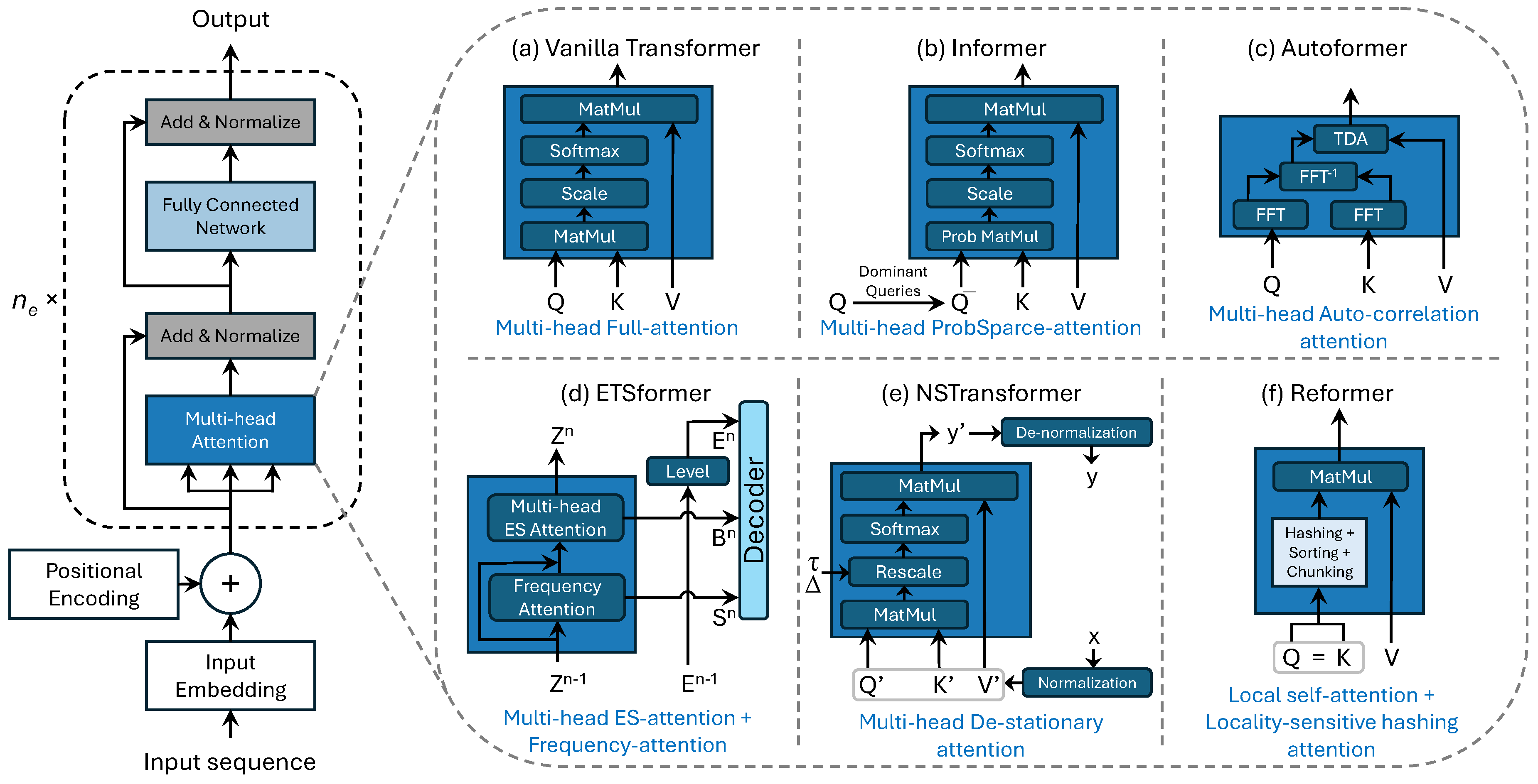
Figure 2.
Architecture of transformer-based models for probabilistic time series forecasting and their tokenization process.
Figure 2.
Architecture of transformer-based models for probabilistic time series forecasting and their tokenization process.
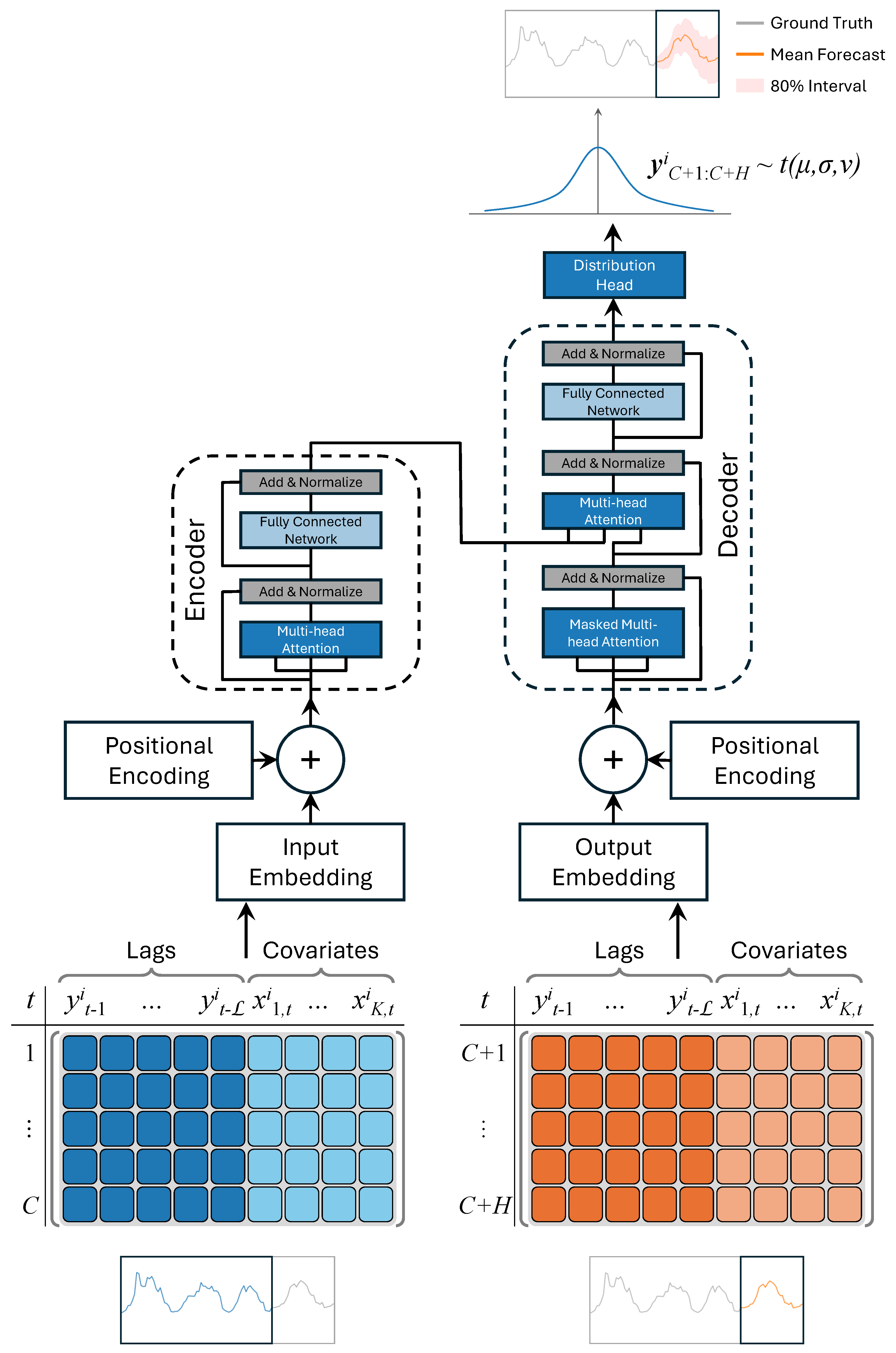

Table 1.
Lags and explanatory variables used in the forecasting models, including time-related features, price data, SNAP activities, event indicators, and hierarchical identifiers.
Table 1.
Lags and explanatory variables used in the forecasting models, including time-related features, price data, SNAP activities, event indicators, and hierarchical identifiers.
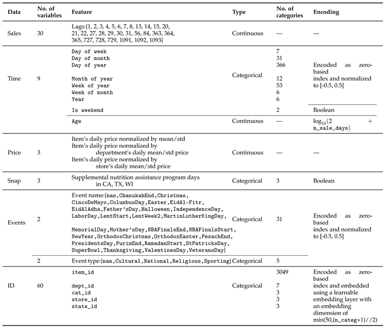
Table 2.
Model’s hyperparameter search spaces used in HPO.
| Hyperparameter | Range | |
|---|---|---|
| Transformer, Autoformer, Informer | ETSformer | |
| NSTransformer, Reformer | ||
| Context length | ||
| Batch size | ||
| Number of encoder layers | — | |
| Number of decoder layers | — | |
Table 3.
Hyperparameter settings applied during the tuning process with the Optuna framework.
| Parameter | Value |
|---|---|
| Number of trials | 10 |
| Number of epochs | 10 |
| Number of batches per epoch | 50 |
| Number of samples | 20 |
| Validation function | Mean Weighted Quantile Loss (MWQL) |
Table 4.
Parameter-specific configurations applied to each of the Transformer-based models.
| Parameter | Transformer | Autoformer | ETSformer | Informer | NSTransformer | Reformer |
|---|---|---|---|---|---|---|
| Prediction length of decoder | 28 | |||||
| Distribution output | Student’s t | |||||
| Loss function | Negative log likelyhood | |||||
| Learning rate | ||||||
| Size of target | 1 | |||||
| Scale of the input target | mean | std | std | std | — | std |
| Lags sequence | [1,2,3,4,5,6,7,8,13,14,15,20,21,22,27,28,29,30,31,56,84,363,364,365,727, | |||||
| 728,729,1091,1092,1093] | ||||||
| Dimensionality of Transformer layers | 32 | — | 64 | 64 | — | 64 |
| Number of attention heads | 2 | |||||
| Feedforward hidden size | 32 | 32 | — | 32 | 32 | — |
| Activation function | gelu | relu | — | relu | gelu | — |
| Dropout for fully connected layers | ||||||
| Moving average window | — | 25 | — | — | — | — |
| Autocorrelation factor | — | 1 | — | — | — | — |
| Number of layers | — | — | 2 | — | — | — |
| K largest amplitudes | — | — | 4 | — | — | — |
| Embedding kernel size | — | — | 3 | — | — | — |
| Attention in encoder | — | — | — | ProbAttention | — | — |
| Use distilling in encoder | — | — | — | True | — | — |
| ProbSparse sampling factor | — | — | — | 5 | — | — |
Table 5.
Optimal hyperparameter configurations obtained through the Optuna framework for each Transformer-based model.
Table 5.
Optimal hyperparameter configurations obtained through the Optuna framework for each Transformer-based model.
| Hyperparameter | Transformer | Autoformer | ETSformer | Informer | NSTransformer | Reformer |
|---|---|---|---|---|---|---|
| Without features | ||||||
| Context length | 28 | 28 | ||||
| Batch size | 128 | 64 | 128 | 256 | 256 | 64 |
| Number of encoder layers | 16 | 16 | — | 16 | 4 | 4 |
| Number of decoder layers | 2 | 8 | — | 16 | 8 | 4 |
| Best MWQL value | ||||||
| With features | ||||||
| Context length | 28 | 28 | 28 | |||
| Batch size | 256 | 256 | 128 | 128 | 256 | 32 |
| Number of encoder layers | 8 | 4 | — | 2 | 4 | 16 |
| Number of decoder layers | 4 | 4 | — | 2 | 4 | 2 |
| Best MWQL value | ||||||
Table 6.
Overall performance comparison of Transformer-based models across point and probabilistic forecast metrics.
Table 6.
Overall performance comparison of Transformer-based models across point and probabilistic forecast metrics.
| Point forecast metrics | Probabilistic forecast metrics | |||||||
| Model | MASE | NRMSE | WQL | WQL | WQL | MWQL | MAE Coverage |
|
| Transformer | Without features | |||||||
| With features | ||||||||
| Autoformer | Without features | |||||||
| With features | ||||||||
| ETSformer | Without features | |||||||
| With features | ||||||||
| Informer | Without features | |||||||
| With features | ||||||||
| NSTransformer | Without features | |||||||
| With features | ||||||||
| Reformer | Without features | |||||||
| With features | ||||||||
Table 7.
Point forecasting accuracy of models across different forecast horizons.
| MASE | NRMSE | ||||||||
| Model | 1 step | 7 steps | 14 steps | 21 steps | 1 step | 7 steps | 14 steps | 21 steps | |
| Transformer | Without features | ||||||||
| With features | |||||||||
| Autoformer | Without features | ||||||||
| With features | |||||||||
| ETSformer | Without features | ||||||||
| With features | |||||||||
| Informer | Without features | ||||||||
| With features | |||||||||
| NSTransformer | Without features | ||||||||
| With features | |||||||||
| Reformer | Without features | ||||||||
| With features | |||||||||
Table 8.
Probabilistic forecasting accuracy of models across different forecast horizons.
| MWQL | MAE Coverage | ||||||||
| Model | 1 step | 7 steps | 14 steps | 21 steps | 1 step | 7 steps | 14 steps | 21 steps | |
| Transformer | Without features | ||||||||
| With features | |||||||||
| Autoformer | Without features | ||||||||
| With features | |||||||||
| ETSformer | Without features | ||||||||
| With features | |||||||||
| Informer | Without features | ||||||||
| With features | |||||||||
| NSTransformer | Without features | ||||||||
| With features | |||||||||
| Reformer | Without features | ||||||||
| With features | |||||||||
Disclaimer/Publisher’s Note: The statements, opinions and data contained in all publications are solely those of the individual author(s) and contributor(s) and not of MDPI and/or the editor(s). MDPI and/or the editor(s) disclaim responsibility for any injury to people or property resulting from any ideas, methods, instructions or products referred to in the content. |
© 2025 by the authors. Licensee MDPI, Basel, Switzerland. This article is an open access article distributed under the terms and conditions of the Creative Commons Attribution (CC BY) license (http://creativecommons.org/licenses/by/4.0/).
Copyright: This open access article is published under a Creative Commons CC BY 4.0 license, which permit the free download, distribution, and reuse, provided that the author and preprint are cited in any reuse.


