
Submitted:
21 August 2025
Posted:
22 August 2025
You are already at the latest version
Abstract
An exposed sedimentary succession, ca 115 m of 1000 m, from the Eastern Carpathian foredeep was for the first time analysed using facies analysis and scale and time inde-pendent sequence stratigraphy methods to reveal the depositional environment and its cyclic sedimentation. The outcropping deposits, dated on the basis of molluscs, forami-nifera, and ostracods are uppermost Volhynian (late Serravalian). The three recurrent facies associations we distinguished indicate a high energy shoreface – transition to offshore environment, episodically affected by storms. Five decametre thick high fre-quency sequences (HFS1–5), at most of 4th rank, bounded by maximum regressive sur-faces, were defined in the studied interval. The maximum thickness of Volhynian (12.65 – 12 Ma) deposits in the area, known both from well sites and outcrops, allowed to estimate the sedimentation rate at ca 1.5 mm/yr. The fossil content shows that entire sedimentary succession deposited in very shallow to shallow water during all Volhyn-ian. The time interval we studied was ca 75 kyr, so that average time of a HFS is ca 15 kyr. At this scale, considering that both high subsidence and Eastern Paratethys sea-level rise added to accommodation, the sediment supply must have been responsi-ble of cyclic nature of sedimentation, which, in turn, must have been controlled by precession climatic changes in the source area. The estimated time of a HFS is smaller than a precession cycle, but better dating might support or infirm this hypothesis.
Keywords:
Dacian Basin
; shallow water
; high-energy shoreface
; cyclic sedimentation
; high frequency sequences
; high accommodation
; precession climatic change
1. Introduction
The late Middle Miocene (Volhynian substage of Sarmatian s.l. stage) sedimentary succession which makes the topic of this paper was deposited in the northern part of the Romanian Eastern Carpathian foredeep, belonging to the so-called Dacian Basin, one of the sub-basins defined in Eastern Paratethys (Figure 1A).
After the rising of mountain ranges consequent to Alpine orogeny, by the end of Eocene, the former Tethys Ocean was succeeded by Mediterranean Sea, to the south, and the Paratethys Sea, the latter covering large areas of Europe and Asia [1,2]. The two successors of the Tethys Ocean, only intermittently communicated, so that for each of them a different chronostratigraphic scale was developed; the Mediterranean one is considered standard, while the one for Paratethys is regional. The different areas of the Paratethys Sea had different evolution both in time and in space. In time, by geodynamic and palaeobiologic data, four evolution stages were recognized [3,4]: Protoparatethys (early to middle Oligocene), Eoparatethys (late Oligocene to Early Miocene), Mesoparatethys (late Early Miocene to early Middle Miocene) and Neoparatethys (Middle Miocene to Pleistocene). In space, three main regions were distinguished, Western Paratethys, Central Paratethys, and Eastern Paratethys. The Western Paratethys, mostly covering the North Alpine Foreland, ended its evolution in Early Miocene [5]. The Central Paratethys evolved up to the beginning of Late Miocene (end of Sarmatian sensu stricto defined by Suess) in the Alpine-Carpathian foreland Basin and Pannonian Basin, giving place to Pannonian Lake which was filled up around Pliocene. The Eastern Paratethys, extending from Romanian Carpathian foreland to the east of Caspian Sea, continued to evolve, while shrinking, until Pleistocene, its remnant being still represented in Black Sea, Caspian Sea and Aral Sea [6]. The part of Miocene Eastern Paratethys on Romania territory is known as Dacian Basin, although there are authors which restrict its significance only to the Southern Carpathian foredeep e.g., [7,8].
There are only a few papers regarding the Miocene sequence stratigraphic evolution of the Eastern Paratethys covering Carpathian foreland, most of them discussing the part of the basin in South-eastern and Southern Carpathian foreland [8,9,10,11,12,13,14], even fewer for its northern area [15,16,17]. The aim of this paper is to make a step forward in the sequence stratigraphy knowledge of the early Sarmatian sedimentary succession from the northern part of Eastern Carpathian foreland.
2. Geological Setting
The study area (Figure 1B) is located within the foredeep zone of Eastern Carpathian (EC) foreland basin system [8,15,16,18].
The studies in the Eastern Carpathian (EC) foreland on Romania territory began after the mid-nineteen century, most of them focusing on general lithostratigraphy, biostratigraphy, and chronostratigraphy. Hundreds of papers were published in periodicals of local significance, mostly in Romanian, but also in French, German or Russian languages, dealing with lithological description and palaeontological fossil content analyses, as well as with biostratigraphic dating of exposed deposits. Much lesser information come from bore holes data, even lesser from seismic data. It is beyond our scope to exhaustively present them, but we consider our duty to mention this, considering that some of the previous results are recycled and published as novelties without proper citations. Among the main results acquired during more than 160 years of work, especially for the northern area of the EC foreland, we consider the follow the most important:
1) in the sedimentary succession, three megacycles were defined, namely Vendian (Ediacaran) – Devonian, Cretaceous – middle Eocene, Middle Miocene – Late Miocene [19]; within these megacycles, different cycles, bounded by unconformities were defined;
2) only the newest deposits (late Middle Miocene) of the last megacycle are exposed in the area, most of the works published in the last over 160 years being dedicated to their study; the exposed deposits were initially divided based on their lithology and fossil content in three units [20], ascribed to the regional stage Sarmatian (sensu lato defined by Barbot de Marny), which latter were given names [21], Volhynian, Bessarabian, Khersonien; worthy to mention that Sarmatian s.l. has a larger time range than Sarmatian s.s., the latter corresponding only with Volhynian and early Bessarabian of the former [22,23];
3) a lateral lithology and fossil content change was remarked in the exposed deposits, three or four ”facies” and/or biofacies being distinguished (e.g., [7,19,24,25]), namely littoral, neritic-arenitic, neritic-pelitic, and reef facies (Figure 1B);
5) the last megacycle, which lasted longer toward the south, was sedimented in the foreland basin system developed as a consequence the last EC Moldavian tectogenesis (regional age Volhynian) [15,16]; the four depozones of a foreland basin system defined by [29] were recognized [15,16] (Figure 1C); the upper Volhynian deposits overlay lower Volhynian folded deposits after an angular unconformity [17,26] in the wedge top depozone.
The Volhynian sedimentary succession analysed in this work belongs to the Middle Miocene (regional stage Badenian) – Pleistocene megacycle, that lasted not later than Maeotian (latest Tortonian – early Messinian) in the northern part of EC foreland, within which two unconformities were defined [31,32]: in between Badenian and Sarmatian; in between Bessarabian and Khersonian.
Although the cyclic nature of sedimentary cover at different scale is acquainted by decades, a proper sedimentological study using the standard facies analysis as well as a sequence stratigraphic approach lack. Here we present the results of such analyses made at the outcrop scale where the highest frequency sequences were recognized in the Șomuz Formation (upper Volhynian) sedimentary succession. For this study we chose the best exposure in the area (ca 115 m stratigraphic thickness) that was biostratigraphically dated before in the stratotype of the named formation [28].
3. Materials and Methods
The methods used in this study are:
- 1)
- Field analyses made in several field seasons during which detailed logs and sampling of outcrops were made in the Șomuz Formation stratotype area. Sedimentological investigations consisted in standard bed-by-bed logging after Nemec [33]’s methodology and photo shootings along Livijoara creek. A rough grouping of facies in facies associations was performed in the field, the latter being laterally traced on the photos where inaccessible. The descriptive sedimentological terminology is after [34,35,36,37] while for abbreviation we used the method of Miall [38] who uses capitals for lithology and smalls to abbreviate the sedimentary structure (e.g., Shcs means sands with hummocky cross stratification). Facies analysis and sedimentary process interpretation lead to the presented palaeodepositional environment interpretation based on existing facies models [39,40,41,42,43].
- 2)
- During sedimentary succession logging, several samples were collected for micro- and macrofauna analyses and photos were shot. Their fossil content, as well as the one known from previous papers (e.g., [28] was used for biostratigraphic age determination. The zonations proposed by [28,44,45,46,47], on the basis of molluscs, foraminifera and ostracods, were used. Some palaeoecological inferences were made taking in consideration the habitats of contemporary relatives of some taxa (molluscs and foraminifera).
- 3)
- The sedimentary succession was also studied by sequence stratigraphic point of view. For this purpose, we followed the terminology and model- and scale-independent work method especially useful at outcrop scale [48,49,50,51] where stratigraphic sequences are defined on the basis of their stratal stacking patterns and bounded by recurrent sequence stratigraphic surfaces irrespective of their allogenic or autogenic origin. Such a method can be applied at any temporal and space scale (form outcrop to seismic scale), allowing to avoid the confusions that can occur when the classic methods from the dawn of rather low-resolution seismic stratigraphy, proposed in 1970s-1980s, e.g., [52,53,54,55,56], are used. The data gathered from natural exposures have the disadvantage as being difficult to correlate, considering their sparsely distribution, as well as the possibility of estimating the extension significance of stratigraphic surfaces, being they local or regional. Accordingly, unconformities are considered here relevant sedimentologic hiatuses [51], even if they do not cover temporal gaps long enough to be biostratigraphically proven. We identified five decametre-thick sequences which we consider high frequency sequences (HFS).
4. Results
4.1. Biostratigraphic Data
As we mentioned before, the biostratigraphic dating was made on the basis of the samples whose fossil content (ca 115 m; Figure 2) consists of molluscs (bivalves and gastropods), foraminifers, and ostracods. Among the molluscs with biostratigraphic value we mention (Figure 3): Podolimactra eichwaldi, Plicatiformes plicatus, P. latisulcus, Potamides disjunctus, Tiaracerithium pictum. These are new accepted names, proposed by [57,58,59], for the former Mactra eichwaldi, Plicatiforma plicata, P. latisulca, Potamides mitralis.
Podolimactra eichwaldi Range Zone is superpose on Volhynian substage, while P. eichwaldi – Plicatiformes praeplicatus and P. eichwaldi – Plicatiformes plicatus Concurrent-range Zones with lower Volhynian and upper Volhynian, respectively, according to Kojumdgieva et al. [46]. The occurrence of Sarmatimactra pallasi (former Mactra vitaliana pallasi) would coincide with the Bessarabian beginning, while the presence of Plicatiformes latisulcus with the uppermost Volhynian. However, the biozonation proposed by [28,44,45] (Figure 2) does not recognize any range zone, but an Assemblage Zone with Podolimactra eichwaldi and Plicatiformes (former Plicatiforma) plicatus. Tiaracerithium pictum is the revised and accepted name of former Potamides mitralis, P. nimpha, and P. bicostatus, previously defined as different species (e.g., [44]), as shows Harzhauser et al. [58]. Its range zone extends all Volhynian and the lower part of Bessarabian (Figure 2). All biozonations mentioned before indicate that the studied deposits are uppermost Volhynian.
Among the foraminifera with biostratigraphic value we mention (Figure 4): Elphidium hauerinum; E. rugosum; E. macellum; Porosononion subgranosus; Pseudotriloculina (former Quinqueloculina) consobrina. They belong to the ACME Zones of Elphidium rugosum and Pseudotriloculina consobrina [44,45,60]. Additionally, the ostracod fauna is characteristic to early Sarmatian assemblages of Vienna Basin [61], Polish Carpathian Foredeep [62], and Eastern Carpathian Foredeep [60,63]. In the studied outcrop, the ostracod assemblage consists of Cyprideis pannonica, Loxoconcha minima, Aurila mehesi, and Callistocythere postvallata. Other biostratigraphically important ostracod species (Aurila notata) was identified in the neighbourhood outcrops by [64]. The latter places the studied deposits in the NO12 Neocyprideis (N.) kollmani – Aurila notata Zone of Jiříček and Říha [47], indicating the lower Sarmatian in Vienna Basin.
4.2. Paleoecologic Inferences
The macro- and microfossil assemblages allowed us to infer some paleoecologic conditions, among the most important for our study being the basin deepness. Such inferences are made on the basis of contemporary fauna habitats. For instance, Actaeocina, which occurs in the sedimentary succession (Figure 4), is a small predatory gastropod living in shallow waters (on muddy or sandy bottoms) of different salinities [65].
Donax trunculus, a possible contemporary relative of Donax dentiger, use to populate beaches between 0-2 m deep on Mediterranean and 0-6 m on Atlantic coasts, respectively, being an exclusive species of Superficial Fine Sand (SFS) biocenosis, strictly dependent by a certain sediment grain size (fine to medium sand) [66]. Signorelli [59] shows that mactrids prefer muddy subtidal sediment to burry in. Polititapes aureus, a contemporary relative of Polititapes gregarius tricuspis, can be found in water of 10 to 35 m deep (https://obis.org/taxon/246150). Potamides disjunctus was a highly frequent species in shallow littoral to sublittoral settings, preferring sandy bottoms [58]. In the Mediterranean environment, Gibbula populates shallow waters from the lowest level of spring tides down to 73 m [68].
The microfossil assemblages yielded by samples not only from the studied area and neighbourhoods, but also from several well sites (e.g., down to -1392 m in Suceava area; Figure 1B) consists of foraminifers (Elphidium, Porosononion, Quinqueloculina, and Ammonia genera [28,44,60,69]), and ostracods (Cyprideis, Loxoconcha, Aurila, and Callistocythere [60,63,64]). Both foraminifera and ostracods indicate shallow water environments. For instance, Elphidium and Quinqueloculina are epifaunal organisms living in the oxic, inner shelf high energy environments [70,71,72,73], while Ammonia beccarii prefers water depths between 0-50 m.
4.3. Sedimentary Environments
Three recurrent facies associations (FA1-3) were defined in the studied sedimentary succession along Livijoara Creek which will de described and interpreted bellow. Their characteristics, compared with existing facies models [40,41,42,43], indicate a high-energy, episodically affected by storms, shoreface – transition to offshore sedimentary environment (Figure 5). This facies model enhances the vertical facies successions in relation with the depth of fairweather and storm-wave base. The water shallowness is also proved by both macro- and microfossil content (Chapt. 4.2).
Facies association 1: greyish-blue sandy mud and muddy sands with RCL of transition zone to offshore
Description: The peculiarity of this facies association is given by the greyish-blue sandy mudstone with lenticular cm-dm thick bioclastic accumulations and muddy sands. The most common sedimentary facies of this association are: dm to thick greyish-blue sandy mudstone (M), shell beds (SB) with Tiaracerithium, Potamides, Acteocina, Obsoletiformes, Polititapes, Donax among others, muddy sands with wave ripple cross lamination (Swrcl), but also some rare thin beds (<15 cm) of sands with hummocky cross stratification (HCS), resting on shell beds. Thin interlayers (one shell thick) of bioclastics may also occur independent of sands. The mudstone thicknesses decrease upward from 50-60 cm to < 10 cm.
Interpretation: The accumulation of siltstone facies with flat beds indicates an environment with calm waters, somewhat deeper than in the shoreface area and the conditions of a suspension sedimentation. Worthy to mention that most of the microfossil content of the studied sedimentary succession, consisting mainly from benthonic foraminifera (e.g., Ammonia, Porosononion, Elphidium, Quinqueloculina), come from the mudstones of this FA and indicate shallow water (infra- to upper circalittoral environments). In the same time, we have not observed bioturbation neither in mudstone, nor in muddy sands. The role of storms in shell beds formation was tackled by Kreisa and Bambach [74] among many others. They are seen as reworked and winnowed rather than in place accumulations, resting on sharp erosional surface. Usually, the shells are oriented parallel to bedding or aligned if they have a suitable morphology (such is of Tiaracerithium).
The Swrcl and Shcs, the latter especially when follow the shell beds, indicate periods of storm waves and currents events followed by periods of calmer sedimentation which allowed the micro-epifauna and shallow micro-infauna to thrive. A more detailed discussion on Shcs will be given in FA2 interpretation. The important participation of Swrcl and Scrcl facies in this association suggest the frequent lowering of wave base, probably during storms. According to the models used [40,41,42,43], we consider this association as a record of a transition to offshore subdomain. In the same time, although this FA1 represent the deepest sedimentation sub-environment in the studied succession, the lack of bioturbation, the high frequency of Swrcl and Scrcl, and also Shcs with shelly storm lags, as well as the sandier nature of mudstones indicate a high energy transition zone.
Facies association 2: sands with HCS of lower shoreface
Description: This association contains mostly fine to very fine sands, greyish muddy sands, and mm-cm thick mudstone interlayers. The most frequent distinguished facies are sands with wave and current ripple cross lamination (Swrcl, Scrcl), with HCS (Shcs), with low angle cross stratification (Slacs), and with plane-parallel stratification (Spp). Shcs may grade lateral in Swrcl, the later filling up the depression between hummocks, or may be truncated by Swrcl which can reach sub-metric thickness. Ripple profiles are well preserved in many situations under thin (mm to cm thick) continuous or discontinuous mud drapes. Sands with cross stratification (Stcs) may also occur as isolated sets. The Shcs are fine or very fine and may occurs either as simple sets of 20-30 cm or as thicker (sub-metric) amalgamated units. Where could be measured, the wave length between two swales was 1-2 m. Some of these units are truncated by undulating surfaces bounding intervals characterized by Swrcl.
Interpretation: Among the facies described, Shcs is considered by most authors a diagnostic for storm waves in shallow waters. Other opinions exist, e.g., [75,76], but here we take the mentioned interpretation as granted, considering the macro- and microfossil content (e.g., Tiaracerithium, Gibbula, Duplicata, Plicatiformes, Polititapes, and Quinqueloculina, Ammonia, Elphidium, Porosononion, respectively) in resedimented beds or in mudstone interlayers of FA1. The mentioned fossil content indicates the deepest environment of entire sedimentary succession, being a benthic mixture of infralittoral and upper circalittoral individuals. The formation of hummocky cross stratification (HCS) is one of the important topics in process sedimentology since it was defined by Harms et al. [34]. Strong oscillatory currents [35,39,77,78,79,80] with a unidirectional component (e.g., [81,82]) which may be a geostrophic current [83] were proposed as formation mechanisms and reproduces in laboratory experiments [84,85,86]. HCS represent the internal structure of large (meter to several meters diameter) circular to ellipsoidal dm high mounds (hummocks) separated by similar plan form depressions (swales), so that it consists both in large convex and concave laminae sets. Both 3D swales and hummocks with their internal structure (swaley and hummocky cross stratifications, SCS and HCS) are primary sedimentary structures highly recognized as diagnostic for oscillatory currents generated by storm waves in shallow marine environments. Such topography is built during storms, so that it often occurs above the average storm wave base, but below fair-weather wave base, considering the mounded relief may be readily eroded by normal waves. The Slacs may represent distal portions of large scale Shcs. The intervals consisting of Swrcl and Scrcl indicate returning to normal conditions, yet characterized by high energy proven by the frequent Scrcl sets, while the thin draping or lenticular thin mudstone layer short periods of quiet sedimentation under the wave base.
Based on the existing models presenting facies associations where Shcs is well represented [40,41,42,43], but also on the scarce presence of mudstone, we consider that these deposits were sedimented in the lower shoreface of a high energy coast episodically hit by storms.
Facies association 3: sands with TCS and SCS of upper shoreface
Description: The facies belonging to this association consist mainly of coarse to medium, well sorted, yellowish sands without matrix. Rare interlayers of thin mudstone and bioclastic material, may also occur. The most frequent facies are: sands with trough cross stratification (Stcs), containing shell hash, sands with swaley cross stratification (Sscs), sands with plan-parallel stratification (Spp), sands with current ripple cross lamination (Scrcl). Convolute lamination was also observed in several cases. Stcs and Sscs give the characteristic note to this association. The Stcs occur in sets of 30-50 cm thick bounded by erosive surfaces, while Sscs as singular sets of 20-30 cm thick and sub-metric width. Scrcl occur as cosets of sets of 10-15 cm thick bounded by slightly undulated surfaces.
Interpretation: This mostly well sorted sandy facies association indicates sedimentary processes characterized by high energy. The swaley cross stratification (SCS) is the internal structure of circular to ellipsoidal depressions (swales) formed among mounds with similar planforms (hummocks). The occurrence of only swaley cross stratification is a matter of smaller preservation potential of convex structures (hummocks) under the conditions of energetic processes, likely the mounded relief being readily eroded by normal waves [86,87,88,89]. Also, bioclasts (predominantly gastropods of Tiaracerithium and Potamides or Plicatiformes and Polititapes bivalves) are concentrated sometimes onto erosive bases of SCS indicating storm lags.
Stcs sets are the result sedimentation in complicated bar-trough systems created under the action of longshore, onshore and/or "rip" currents hosting medium scale 2D and 3D megaripples in the upper shoreface area [40,41,42,43,90]. These sets, accumulated during fairweather conditions, are truncated by erosive surfaces bounding Sscs and Spp. The high-rate transport and accumulation during storms over deposits not yet consolidated creates instability at the interfaces between the sands accumulated in different stages, the consequence being the formation of convoluted structures [91] observed in the studied outcrops.
The sedimentary processes interpreted on the basis of the described sedimentary facies are characteristic of the upper shoreface subdomain characterized by the permanent action of fairweather waves, as well as by the periodic incidence of storm surges. Idealized models of this subdomain have been proposed [40,41,42,43].
4.4. High Frequency TR Sequences
The three FAs presented above may occur gradationally on top of each other in coarsening- and shallowing upward trends (Figure 5). Such a gradational succession suggests a continuous sedimentation associated with progradation of the shoreface – transition to offshore depositional system accompanied by a regressive shoreline. The opposite situation also occurs, where a change from a shallow water to a deeper water sedimentation, associated with a finning upward trend, indicates the depositional system retrogradation accompanied by a transgressive shoreline. Both shallowing and deepening upward trends are the results of the relationships between accommodation and sedimentation, a highly debated topic in literature recently reviewed by Catuneanu [92]. The former situation occurs when sedimentation outpaces accommodation, while the latter when the accommodation outpaces the sedimentation. In the studied succession, the shallowing upward intervals may be one order thicker than the deepening upward ones. The ShU and DU intervals are bounded rather by nonerosive surfaces, although some dm-thick shell beds might rest onto erosive surfaces. Because of the limited exposure we could not trace them laterally more than 1-2 m, so that this hypothesis remains to be proven. As the interpreted depositional environment shows, the most proximal sub-environments (foreshore, backshore) lack from succession, so that the position of the examined deposits should have been at some distance from the shore where the development of subaerial unconformities was rather unlikely. Accordingly, here we chose to use the transgressive – regressive sequence model [93] bounded by maximum regressive surfaces.
Five high frequency sequences of were defined in the ca 115 m exposure (Figure 6), abbreviated as HFS1-HFS5. These cycles are decametre-thick regularly repeated successions of facies associations. Four of HFS are dominated by the thicker regressive deposits (Figure 6). In HFS4 the transgressive and regressive deposits have almost equal thicknesses. In same sequence, the upper shoreface lacks. It seems that there is a thinning upward trend from HFS1 to HFS3 followed by a thickening upward trend from HFS3 to HFS5.
5. Discussion
The cyclic nature of the deposits studied in this paper is obvious. The high frequency sequences are part of Volhynian – Bessarabian cycle, belonging to the last sedimentary ”megacycle” defined for the Carpathian foreland. This “megacycle” includes several unconformities proven on different criteria [19,32], as we mentioned in Chapt. 2 The unconformity between Badenian and Sarmatian was established based on sudden change of micro- and macrofossils from marine to brackish assemblages [94], and occurs in the entire Dacian Basin of Eastern Paratethys. In between middle Sarmatian (Bessarabian) and upper Sarmatian (Khersonian) there is a disconformity which was observed in field, especially toward the Carpathians where upper Bessarabian lacks [31]. Consequently, the HFSs belong to Volhynian – Bessarabian cycle.
If we were to rank the entire sedimentary succession of the foreland, then the three megacycles would be 2nd rank sequences, and the Volhynian – Bessarabian sedimentary cycle would be a 3rd rank sequence. Similar ranking was proposed for western Central Paratethys [95] where the Sarmatian s.s. (correlating with Volhynian – lower Bessarabian) sedimentary succession was equivalated with the global cycle TB2.6 (3rd rank). Consequently, the HFS1-5 presented in this paper may be 4th rank at most. Worthy to mention here that the entire Volhynian sedimentary succession known from wells and outcrops is ca 1600 m in the proximal foredeep (Figure 1B), but the deposits are always of shallow water as indicates the fossil content mentioned in Chapt. 4.2. Older high frequency sequences (but still Volhynian) of shoreface deposits are also preserved in the wedge-top depozone northward of Solca [17] (Figure 1B). Equivalent age deposits are one order thinner away from Eastern Carpathians (Figure 1B).
At the scale of the outcrops, although it is possible to recognize the sequences, it is difficult, if not impossible, to interpret the controlling factors, because the extension of the bounding sequence stratigraphic surfaces cannot be estimated as they rather reflect importance of the local controls on the accommodation and sedimentation [50]. In the same time, at any scale, the global controls on accommodation and sedimentation may combine in indefinite ways with the local ones, the resulting sequences reflecting both categories. Moreover, for the lower rank sequences, such the ones we discuss here, the controls may be both allogenic and autogenic [50,51]. Autogenic sequences are more common in the case of deltaic systems, but the system defined by us is shoreface – transition to offshore, so we may ignore this hypothesis. The shoreface – offshore system is very sensitive to allogenic changes in the accommodation space, controlled by sea-level changes and tectonics [54,55]. Sedimentation reflects the supply of sediment to a certain depositional area but also the energy flux of the environment [92]. The former depends on climate, erosional processes, size of source areas, the existence of intermediary traps along the sediment transport routes in the source areas (e.g., [96]), the source area itself being a result of tectonic uplifting.
Because of the described situation, the discrimination of the controls for the studied sedimentary succession must be taken with caution, each of them having its own timing, although tectonics had the lead.
5.1. Paratethys Sea-Level Control on Accommodation
The placement of the sequence stack defined in the studied outcrops in a regional and global context of sea-level oscillation (Figure 7) is very much an attempt to estimate its role, on one hand, and to discriminate the role of the tectonic factor, on the other, given that the sedimentary basin was the Eastern Carpathian foredeep created after the intra-Volhynian Moldavian tectogenesis.
5.2. Tectonic Control on Accommodation
The sedimentation took place during the Moldavian major deformation of Eastern Carpathian [99,100], responsible for the main nappe emplacement, when the new foreland basin system was organized [15,16]. The nappe load use to create a depositional space due to flexure of continental lithosphere undergoing subduction, forming accretionary wedges and foreland basin system (e.g., [29]). During convergence, sediment deposited in foredeep may be incorporated in the thrust belt, uplifted and eroded as it was the case during with early Volhynian deposits [17,26].
In the area we discuss here, the last thrusting event was intra-Volhynian, considering the angular unconformity between lower Volhynian folded deposits and undeformed upper Volhynian deposits in wedge top depozone located northward of Solca [17,26].
It is very likely that accommodation space is mostly due to tectonics, an echo of the accelerated subsidence caused by Moldavian major thrusting event. One more complexity is added by the along Carpathian foredeep migration of the depocenters with an average rate of 380 km/Myr in Volhynian-Bessarabian [18]. Such a temporary depocenter must have been in the proximal foredeep, south-westward of the study area (Figure 1B). The depocenter migration was driven by the diachronic thrusting event along the Carpathians, which in Polish Carpathians, for instance, was Badenian, while in Romanian Carpathians was intra-Sarmatian, still younger from the north to the south [99,101].
5.3. Controls on Sediment Supply
During late Badenian – Sarmatian (15-11 Ma), the Carpathians rose above the sea-level while being shaped by weathering and erosion [102]. The latter authors showed that in the mentioned time span ca 4 km of exhumed deposits were eroded in the north Eastern Carpathians, so that the Carpathians maintained a low-altitude [103]. The tectonic landscape of Carpathian source area undergone the effects of opposite forces, tectonic uplifting and denudation, the latter highly dependent of climate. However, the interaction between the two controls is highly variable, the sediment efflux response to tectonic uplifting being delayed a very long time (106-107 years) in large orogenic systems or rather short time (105 years) for trains of folds in fold-thrust belts (data in [104]). In the same time, if climate (precipitation) is favourable, any tectonic uplifting may be adjusted by aggressive erosion in reactive tectonic landscapes [104]. One of the controls on climate is generated by periodic oscillations of orbital parameters of Earth, known as Milankovitch cyclicity (likely precession cycles), which may have long- to short periods [105], but we lack such information for our study area.
5.4. Cyclicity Modulator in the High Accommodation and Supply Area
Both subsidence (proximal-distal and along-Carpathians) and Eastern Paratethys sea- level rise added to accommodation, the result being a ca 1600 m deposits supplied by uplifting orogen in a rather short time span. As the fossil content both from the wells and outcrops and the interpreted depositional system reveal, there was not a pre-existing bathymetric depression that could have accommodated such a thick package of sediment. Hence, the thicker accumulations of sediment near the thrust line (Figure 1B) mark the position of actively subsiding depocenters and not pre-existing bathymetric troughs.
There are not numerical ages of the Sarmatian substages in Dacian Basin. We do not know the numeric age of Volhynian – Bessarabian boundary, but we may take as guidance the results of magnetostratigraphy and radiometric dating acquired by Vasiliev et al. [106] in Transylvanian Basin (part of Central Paratethys) for Sarmatian s.s. – Pannonian, corresponding with early Bessarabian – late Bessarabian in Eastern Paratethys, as 11.3 Ma. In the Central Paratethys, however, this boundary is placed at 11.6 Ma and considered roughly equivalent with the Serravalian-Tortonian one, that is at 11.63 Ma (e.g., [107,108]). Harzhauser and Piller [95] put the boundary between Volhynian and Bessarabian in top of chron C5An.1n which was calibrated by Ohneiser et al [109] at 12.014 Ma. A provisory boundary between Volhynian and Bessarabian is placed by Raffi et al. [108] at 12 Ma, so we may assume that that Volhynian substage lasted at most 0.65 myr. Data from wells (Suceava, Rӑdӑuți, Fӑlticeni, and Lespezi areas; Figure 1B) and outcrops shows that the maximum thickness of Volhynian deposits in the northern EC foredeep (part of Dacian Basin) is at least 1600 m, but in the studied area would be ca 1000 m [7,27,28,44]. If we consider a constant sedimentation rate (1.5 mm/yr), then the studied interval would represent around 75 kyr, while an average time span of each HFS would be ca 15 kyr. This figure may be improved by better age constraint of the Volhynian substage.
At this temporal scale, in order to explain the development of HFS1-5 in an accommodation created by cumulative effect of tectonic subsidence and Paratethys sea-level rise, we have to look for a short-period modulator of sediment supply to a rather high energy shoreface – transition to offshore environment. Such modulator could have been climate change controlled by precession cycles, which are the closest as time range. To now, no such studies were made for the Eastern Carpathians’ foreland, so this possible explanation is advanced as a likely hypothesis that need further support. However, the interplay of all above-mentioned controls, acting at different cycle periods, produced the sequences described in this paper, further studies being necessary to discriminate each control role.
6. Conclusions
A sedimentary succession in northern part of Eastern Carpathian foreland was for the first time analysed using sedimentology and sequence stratigraphy methods.
- -
- The sedimentary succession represents the uppermost (ca 115 m) interval of a very thick (ca 1600 m) infill of the north part of Eastern Carpathians’ foredeep accumulated during their last major tectonic deformation (Moldavian tectogenesis).
- -
- Based on the molluscs, foraminifera, and ostracods, the sedimentary succession was biostratigraphically dated as uppermost Volhynian (the lower substage of the stage Sarmatian s.l., regionally defined for Eastern Paratethys).
- -
- The fossil content of the both studied interval and from several well sites (down to -1392 m) from neighbouring areas always indicate always shallow water, inner shelf (littoral to sublittoral) environments.
- -
- Three facies associations were defined, greyish-blue sandy mud and muddy sands with RCL of transition zone to offshore, sands with HCS of lower shoreface, and sands with TCS and SCS of upper shoreface, and interpreted as high-energy shoreface – transition to offshore, episodically affected by storms, sedimentary paleoenvironment.
- -
- The vertical recurrence of the three facies association allowed us to define five decametre – thick high frequency sequences (HFS1-5) bounded by maximum regressive surfaces, four of them mostly regressive, one transgressive-regressive types. The HFSs are at most of 4th rank and belongs to the (Volhynian – early Bessarabian, 3rd rank sequence, itself part of the Miocene 2nd rank sequence (“megacycle”).
- -
- The HFS sedimentation occurred in high accommodation setting where both foredeep high subsidence, a consequence of the major deformation of Eastern Carpathians in Volhynian, and Paratehys sea-level rise contributed. The high accommodation was balanced by a high sedimentation rate, so that the depositional environment remained shallow water.
- -
- The time span of the five HFSs was estimated as ca 75 kyr, from the ca 0.65 myr of Volhynian, on the basis of different evidences, each HFS lasting ca 15 kyr.
- -
- To explain the high frequency cyclicity on a high accommodation background at the space and time scale of HFSs we hypothesize as modulator the sediment supply controlled by precession climatic change in Carpathian source area.
- -
- Further studies are necessary in order to confirm the proposed control on cyclic sedimentation or to identify a better one.
Author Contributions
Conceptualization, C.M.; methodology, all authors; investigation, all authors; data curation, C.M., V.I., and S.L.; writing—original draft preparation C.M., A.S.; writing—review and editing, C.M., V.I., S.L. Author A.S. passed away prior to publication of this manuscript. All authors have read and agreed to the published version of the manuscript.
Funding
C.M. and V.I.’s researches were funded by “Alexandru Iona Cuza University” of Iași, grant FCSU. S.L.’s research was funded by Project PNRR C9-I19 “Multiproxy reconstruction of Eurasian Megalakes, connectivity and isolation patterns during Neogene – Quaternary times” code 97/15.11.2022, Contract No. 760115/ 23.05.2023.
Data Availability Statement
Data will be available upon request.
Acknowledgments
The revision performed by three anonymous reviewers is greatly acknowledged.
Conflicts of Interest
The authors declare no conflicts of interest.
References
- Rögl, V.F. Palaeogeographic considerations for Mediterranean and Paratethys seaways (Oligocene to Miocene). Ann. Naturhist. Mus. Wien 1999, 99A, 279–310. [Google Scholar]
- Steininger, F.H.; Wessely, G. From Tethyan Ocean to the Paratethys Sea: Oligocene to Neogene stratigraphy, palaeogeography and palaeobiology of the circum-Mediterranean region and the Oligocene to Neogene basin evolution in Austria. Mitt. Osterr. Geol. Ges. 1999, 92, 92–116. [Google Scholar]
- Seneš, J.; Marinescu, F. Cartes paléogéographiques du Néogène de la Paratéthys centrale. Memoires Bureau Recherches Géologiques et Minières 1974, 78, 785–792. [Google Scholar]
- Rusu, A. Oligocene events in Transylvania (Romania) and the first separation of Paratethys. D. S. Inst. Geol. Geofiz. 1988, 72–73, 207–223. [Google Scholar]
- Seneš, J. Entwicklungsphasen der Paratethys. Mitt. Geol. Gessell. (Wien) 1960, 52, 181–188. [Google Scholar]
- Harzhauser, M.; Landau, B.; Mandic, O.; Neubauer, T.A. The Central Paratethys Sea – rise and demise of a Miocene European marine biodiversity hotspot. Scientific Reports 2024, 14, 16288. [Google Scholar] [CrossRef]
- Saulea, E.; Popescu, I.; Sandulescu, J. Atlas litofaciesal. VI – Neogen; 1: 200 000. Institutul Geologic al României, București, Romania, 1969; map. [Google Scholar]
- Jipa, D.C.; Olariu, C. Dacian Basin. Depositional architecture and sedimentary history of a Paratethys Sea. Geo-Eco-Marina Special Publication no. 3, GeoEcoMar, București, Romania. 2009; p. 264. [Google Scholar]
- Leever, K.A.; Matenco, L.; Rabagia, T.; Cloethingh, S.; Krijgsman, W.; Stoica, M. Messinian sea level fall in the Dacic Basin (Eastern Paratethys): palaeogeographical implications from seismic sequence stratigraphy. Terra Nova 2010, 22, 12–17. [Google Scholar] [CrossRef]
- Munteanu, I.; Matenco, L.; Dinu, C.; Cloetingh, S. Effects of large sea-level variations in connected basins: the Dacian-Black Sea system of the Eastern Paratethys. Basin Research 2012, 0, 1–15. [Google Scholar] [CrossRef]
- Palcu, D.V.; Tulbure, M.; Bartol, M.; Kouwenhoven, T.J.; Krijgsman, W. Badenian-Sarmatian Extinction Even in the Carpathian foredeep of Romania: paleogeographic changes in the Paratethys domain. Global and Planetary Change 2015, 133, 346–358. [Google Scholar] [CrossRef]
- Palcu, D.V.; Vasiliev, I.; Stoica, M.; Krijgsman, W. The end of the Great Khersonian Drying of Eurasia: Magnetostratigraphic dating of the Maeotian transgression in the Eastern Paratethys. Basin Research 2019, 31, 33–58. [Google Scholar] [CrossRef]
- Matoshko, A.; Matoshko, A.; de Leeuw, A.; Stoica, M. Facies analysis of the Balta Formation: Evidence for a large fluvio-deltaic system in the East Carpathian Foreland. Sedimentary Geology 2016, 343, 165–189. [Google Scholar] [CrossRef]
- Matoshko, A.; de Leeuw, A.; Stoica, M.; Mandic, O.; Vasiliev, I.; Floroiu, A.; Krijgsman, W. The Mio-Pliocene transition in the Dacian Basin (Eastern Paratethys): paleomagnetism, mollusks, microfauna and sedimentary facies of the Pontian regional stage. Geobios 2023, 77, 45–70. [Google Scholar] [CrossRef]
- Miclӑuș, C. Geologia deltelor relicte extracarpatice sarmaţiene dintre văile Sucevei şi Bistriţei. PhD Thesis, “Al. I. Cuza” University, Iași, Romania, 2001. [Google Scholar]
- Grasu, C.; Miclӑuș, C.; Brânzilӑ, M.; Boboș, I. Sarmațianul din sistemul bazinelor de foreland ale Carpaților Orientali; Tehnicӑ, Ed.; București, Romania, 2002; p. 407. [Google Scholar]
- Miclӑuș, C.; Grasu, C.; Juravle, A. Sarmatian (middle Miocene) coastal deposits in the wedge-top depozone of the Eastern Carpathian foreland basin system. A case study. An. Șt. ale Univ. „Al.I. Cuza” din Iași, Seria Geologie 2011, 57, 75–90. [Google Scholar]
- Jipa, D.C. Large-scale along-arc sedimentary migration in the Carpathian foredeep. A paleogeographic approach. Palaeogeography, Palaeoclimatology, Palaeoecology 2018, 505, 140–149. [Google Scholar] [CrossRef]
- Ionesi, L. Geologia unitӑților de platformӑ și a Orogenului Nord-Dobrogean; Tehnicӑ, Ed.; București, Romania, 1994; p. 280. [Google Scholar]
- Cobălcescu, G. Studii geologice şi paleontologice asupra unor tărâmuri terţiare din unele părţi ale României; Ed. Stabilimentul Grafic Socecü & Telcu, București, Romania, 1883; p. 161. [Google Scholar]
- Simionescu, I. Contribuțiuni la geologia Moldovei dintre Siret și Prut. Publicațiunile fondului "V. Adamachi” 1903, 9, 73–116. [Google Scholar]
- Steininger, F.; Rögl, F. Paleogeography and palinspastic reconstruction of the Neogene of the Mediterranean and Paratethys. In The geological evolution of the eastern Mediterranean; Dixon, J.E., Robertson, A.H.F., Eds.; Special Publication of the Geological Society; Blackwell Sci. Publ., Oxford, UK, 1984; pp. 659–668. [Google Scholar]
- Vass, D. Numeric age of the Sarmatian boundaries (Seuss 1866). Slovak Geol. Mag. 1999, 5, 227–232. [Google Scholar]
- Paghida-Trelea, N. Microfauna Miocenului dintre Siret și Prut; Ed. Academiei Române, București, Romania, 1969; p. 189. [Google Scholar]
- Ionesi, L.; Ionesi, B.; Roșca, V.; Lungu, A.; Ionesi, V. Sarmațianul mediu și superior de pe Platforma Moldovenească; Ed. Academiei Române, București, România, 2005; p. 557. [Google Scholar]
- Ionesi, B. Cercetări geologice dintre Valea Sucevei și Pârâul Voitinel (Platforma Moldovenească). An. Șt. ale Univ. “Al. I. Cuza” din Iași 1969, 15, 73–82. [Google Scholar]
- Țibuleac, P. 1998. Studiul geologic al depozitelor sarmațiene din zona Fălticeni – Sasca – Răucești (Platforma Moldovenească) cu referire specială asupra stratelor de cărbuni. PhD Thesis, University „Alexandru Ioan Cuza” of Iași, 1999. [Google Scholar]
- Ionesi, V. Sarmațianul dintre Valea Siretului și Valea Șomuzului Mare; Ed. Universitӑții "Alexandru Ioan Cuza" Iași, Romania, 2006; p. 238. [Google Scholar]
- DeCelles, P.G.; Giles, K.A. Foreland basin systems. Basin Research 1996, 8, 105–123. [Google Scholar] [CrossRef]
- Saulea, E. Geologie istoricӑ. Cap. IVB; In Geologie Istorică, Saulea, E., Ed.; Ed. Didacticӑ și Pedagogicӑ, București, Romania, 1967; pp. 621–735. [Google Scholar]
- Ionesi, L.; Ionesi, B. Asupra Vîrstei Nisipurilor de Văleni. An. Muz. Șt. Nat. Piatra Neamț, Seria Geologie-Geografie 1976, III, 139–158. [Google Scholar]
- Ionesi, L.; Ionesi, B. Vue générale sur le Sarmatien des unités de plate-forme de Roumanie. In The Miocene from the Transylvanian Basin Romania; Bedelean, I., Meszaros, N., Nicorici, E., Petrescu, I., Eds.; Ed. Carpatica, Cluj-Napoca. Romania, 1994; pp. 205–216. [Google Scholar]
- Nemec, W. Principles of lithostratigraphic logging and facies analysis. Short Course Compendium. Department of Earth Science, University of Bergen, 1996; p. 25. [Google Scholar]
- Harms, J.C.; Southard, J.B.; Spearing, D.R.; Walker, R.G. Depositional environments as interpreted from primary sedimentary structures and stratification sequences. SEPM Short Course no. 2., Dallas, USA, 1975; p. 161.
- Harms, J.C. Primary sedimentary structures. Ann. Rev. Earth Planet. Sci. 1979, 7, 227–248. [Google Scholar] [CrossRef]
- Allen, J.R.L. Sedimentary Structures: Their Character and Physical Basis; Developments in Sedimentology 30B. Elsevier, Amsterdam, 1984; Volume 2, p. 643. [Google Scholar]
- Collinson, J.D.; Thompson, D.B. Sedimentary structures, 2nd ed.; Chapman & Hall: London, UK, 1989; p. 207. [Google Scholar]
- Miall, A.D. Lithofacies types and vertical profile models in braded river deposits: A summary. Geological Survey of Canada 1977, 5, 597–604. [Google Scholar]
- Walker, R.H. Shelf and shallow marine sands. In Facies Models, 2nd ed.; Walker, R.G., Ed.; Geological Association of Canada, Canada, 1984; pp. 141–170. [Google Scholar]
- Walker, R.G.; Plint, A.G. Wave- and storm-dominated shallow marine systems. In Facies Models. Response to sea level change; Walker, R.G., James, N.P., Eds.; Geological Association of Canada, Love Printing Service Ltd., Stittsville, Ontario, Canada, 1992; pp. 219–238. [Google Scholar]
- Reading, H.G.; Collinson, L.D. Clastic coasts. In Sedimentary environments: Processes, Facies, and Stratigraphy, 3rd ed.; Reading, H.G., Ed.; Blackwell Publishing, Oxford, UK, 1996; pp. 152–280. [Google Scholar]
- Clifton, F.E. A reexamination of facies models for clastic shorelines. In Facies Models Revisited; Posamentier, H.W., Walker, R.G., Eds.; SEPM Special Publ. 84, Tulsa, Oklahoma, USA, 2006; pp. 293–337. [Google Scholar]
- Plint, A.G. Wave- and storm-dominated shoreline and shallow-marine systems. In Facies Models 4; James, N.P., Dalrymple, R.W., Eds.; Geological Association of Canada, GEO text 6, Marquis Book Printing Inc., Canada, 2010; pp. 167–199. [Google Scholar]
- Ionesi, B. Stratigrafia depozitelor miocene de platformӑ dintre Valea Siretului și Valea Moldovei; Ed. Academiei Române, București, Romania, 1968; p. 395. [Google Scholar]
- Ionesi, B. , 1991. Biozonation of the Sarmatian from Moldavian Platform. The celebration days of “Al. I. Cuza” University of Iași (25–26 Oct. 1991) – conference paper.
- Kojumdgieva, E.I.; Paramonova, N.P.; Belokrys, L.S.; Muskhelishvili, L.V. Ecostratigraphic subdivision of the Sarmatian after mollusks. Geologica Carpathica 1989, 40, 81–84. [Google Scholar]
- Jiříček, R.; Říha, J. Correlation of Ostracod Zones in the Paratethys and Tethys. In Shallow Tethys 3: Proceedings of the Internatioanal Symposium on Shallow Tethys 3; Kotaka, T., Ed.; Saito Höonkai: The Saito Gratitude Foundation, Sendai, Japan, 1991; pp. 435–457. [Google Scholar]
- Catuneanu, O.; Galloway, W.E.; Kendall, C.G.S.C.; Miall, A.D.; Posamentier, H.W.; Strasser, A.; Tucker, M.E. Sequence stratigraphy: Methodology and nomenclature. Newsl. Stratigr. 2011, 44, 173–245. [Google Scholar] [CrossRef]
- Catuneanu, O.; Zechin, M. High-resolution sequence stratigraphy of clastic shelves II: controls on sequence development. Mar. Pet. Geol. 2013, 39, 26–38. [Google Scholar] [CrossRef]
- Catuneanu, O. Model-independent sequence stratigraphy. Earth-Sci. Rev. 2019, 188, 312–388. [Google Scholar] [CrossRef]
- Catuneanu, O. Scale in sequence stratigraphy. Mar. Pet. Geol. 2019, 106, 128–159. [Google Scholar] [CrossRef]
- Vail, P.R.; Mitchum, R.M.Jr.; Thompson, S. Seismic stratigraphy and global changes of sea level, Part 3: Relative changes of sea level from coastal onlap. In Seismic Stratigraphy—Applications to Hydrocarbon Exploration; Payton, C.E., Ed.; AAPG Memoir 26; AAPG: Tulsa, OK, USA, 1977; pp. 63–81. [Google Scholar]
- Vail, P.R.; Todd, R.G.; Sangree, J.B. Seismic stratigraphy and global changes of sea level, Part 5. Chronostratigraphic significance of Seismic Reflections: Section 2. Application of Seismic reflection configuration to stratigraphic interpretation. In Seismic Stratigraphy—Applications to Hydrocarbon Exploration; Payton, C.E., Ed.; AAPG Memoir 26; AAPG: Tulsa, OK, USA, 1977; pp. 99–116. [Google Scholar]
- Jervey, M.T. Quantitative geological modeling of siliciclastic rock sequences and their seismic expression. In Sea—Level Changes: An Integrated Approach; Wilgus, C.K., Hastings, B.S., Kendall, C.G.S.C., Posamentier, H.W., Ross, C.A., Van Wagoner, J.C., Eds.; SEPM Special Publication: Claremore, OK, USA, 1988; Volume 42, pp. 47–69. [Google Scholar]
- Posamentier, H.; Vail, P.R. Eustatic controls on clastic deposition II—Sequences and systems tract models. In Sea Level Changes—An Integrated Approach; Wilgus, C.K., Hastings, B.S., Posamentier, H., Van Wagoner, J., Ross, C.A., Kendall, C.G.S.C., Eds.; SEPM Special Publication: Claremore, OK, USA, 1988; Volume 42, pp. 125–154. [Google Scholar]
- Van Wagoner, J.C.; Posamentier, H.W.; Mitchum, R.M.; Vail, P.R.; Sarg, T.S.; Loutit, T.S.; Hardenbol, J. On overview of the fundamentals of sequence stratigraphy and key definitions. In Sea—Level Changes: An Integrated Approach; Wilgus, C.K., Hartings, B.S., Posamentier, H., Van Wagoner, J., Ross, C.A., Kendall, C.G.S.C., Eds.; SEPM Special Publication: Claremore, OK, USA, 1988; Volume 42, pp. 40–45. [Google Scholar]
- Kojumdgeva, E. Les fosiles de Bulgarie. VIII, Sarmatien; Izd. na Lulg. Akad. na Nauk., Sofia, Bulgaria, 1969; p. 223.
- Harzhauser, M.; Guzhov, A.; Landau, B. A revision and nomenclator of the Cainozoic mudwhelks (Mollusca: Caenogastropoda: Batillariidae, Potamididae) of the Paratethys Sea (Europe, Asia). Zootaxa 5272(1), Magnolia Press, Auckland, New Zeeland, 2023; pp. 241.
- Signorelli. J.H. Catalogue of fossil genera of Mactridae (Mollusca: Bivalvia). Journal of Palaeontology 2023, 97, 823–852. [Google Scholar] [CrossRef]
- Dumitriu, S.D.; Loghin, S.; Dubicka, Z.; Melinte–Dobrinescu, M.C.; Paruch–Kulczycka, J.; Ionesi, V. Foraminiferal, ostracod, and calcareous nannofossil biostratigraphy of the latest Badenian–Sarmatian interval (Middle Miocene, Paratethys) from Poland, Romania and Republic of Moldova. Geologica Carpathica 2017, 68, 419–444. [Google Scholar] [CrossRef]
- Gross, M. Mittelmiozane Ostracoden aus dem Wiener Becken (Badenium/Sarmatium, Österreich). Verlag der Österreichischen Akademie der Wissenschaften, Wien, Österreich, 2006; p. 224.
- Aiello, G.; Szczechura, J. Middle Miocene ostracods of the Fore-Carpathian Depression (Central Paratethys, Southwestern Poland). Bolletino della Società Paleontologica Italiana 2004, 43, 11–39. [Google Scholar]
- Ionesi, B.; Chintӑuan, I. Studiul ostracodelor din depozitele volhiniene de pe Platforma Moldoveneascӑ (Sectorul dintre Valea Siretului și Valea Moldovei). D.S. Inst. Geol. Geofiz (1973-1974) 1975, LXI, 3–14. [Google Scholar]
- Loghin, S. Domenii depoziționale și asiociații microfaunistice din partea centralӑ a forelandului Carpaților Orientali. PhD Thesis, “Al.I. Cuza” University, Iași, Romania, 2022. [Google Scholar]
- Semeniuk, V.; Cresswell, I. Species Zonation. In Encyclopedia of Estuaries; Kennish, M.J., Ed.; Encyclopedia of Earth Sciences Series, Springer, Dordrecht, 2016; pp. 613–621. [Google Scholar] [CrossRef]
- La Valle, P.; Nicoletti, L.; Finoia, M.G.; Ardizzone, G.D. Donax trunculus (Bivalvia: Donacidae) as a potential biological indicator of grain-size variations in beach sediment. Ecological Indicators 2011, 11, 1426–1436. [Google Scholar] [CrossRef]
- Ocean Biodiversity Information System. Available online: https://obis.org/taxon/246150 (accessed on 13.03.2025).
- Smith, D.A.S. Some aspects of the biology of Gibbula cineraria (L.) with observations on Gibbula umbilicalis (DaCosta) and Gibbula pennanti (Phil.). (Mollusca: Prosobranchia). PhD Thesis, Durham University, Durham, UK, 1969. [Google Scholar]
- Ionesi, B.; Guevara, I. Studiul depozitelor sarmațiene din forajul 1002 Bӑdeuți (NV Platformei Moldovenești). Bul. Soc. Geol. Rom. 1993, 14, 79–87. [Google Scholar]
- Langer, M.R. Epiphytic foraminifera. Marine Micropaleontology 1993, 20, 235–265. [Google Scholar] [CrossRef]
- Murray, J.W. Ecology and applications of benthonic foraminifera; New York: Cambridge University Press, 2006; p. 426. [Google Scholar]
- Peryt, D.; Gedl, P. Palaeoenvironmental changes preceding the Middle Miocene Badenian salinity crisis in the northern Polish Carpathian Foredeep Basin (Borków quarry) inferred from foraminifers and dinoflagellate cysts. Geological Quarterly 2010, 54, 487–508. [Google Scholar]
- Filipescu, S.; Miclea, A.; Gross, M.; Harzhauser, M.; Zagorsek, K.; Jipa, C. Early Sarmatian paleoenvironments in the easternmost Pannonian Basin (Borod Depression, Romania) revealed by the micropaleontological data. Geologica Carpathica 2014, 65, 67–81. [Google Scholar] [CrossRef]
- Kreisa, R.D.; Bambach, R.K. The role of storm processes in generating shell beds in Paleozoic shelf environments. In Cyclic and Event Stratification; Einsele, G., Seilacher, A, Eds.; Springer-Verlag, Berlin Heidelberg, Germany, 1982; pp. 200–207. [Google Scholar]
- Mulder, T.; Razin, P.; Faugeres, J.-C. Hummocky cross-stratification-like structures in deep-sea turbidites: Upper Cretaceous Basque basins (Western Pyrenees, France. Sedimentology 2009, 56, 997–1015. [Google Scholar] [CrossRef]
- Morsilli, M.; Pomar, L. Internal waves vs. Surface storm waves: a review on the origin of hummocky cross-stratification. Terra Nova 2012, 24, 273–282. [Google Scholar] [CrossRef]
- Leckie, D.A.; Walker, R.G. Storm- and tide-dominated shorelines in Cretaceous Moosebar-Lower Gates interval – Outcrop equivalents of deep basin gas trap in Western Canada. AAPG Bull. 1982, 66, 138–157. [Google Scholar]
- Dott, R.H.; Bourgeois, J. Hummocky stratification: significance of its variable bedding sequences. GSA Bull. 1982, 93, 663–680. [Google Scholar] [CrossRef]
- Cheel, R.J. Grain fabric in hummocky cross-stratified storm beds: genetic implications. J. Sediment. Petrol. 1991, 61, 102–110. [Google Scholar] [CrossRef]
- Cheel, R.J.; Leckie, D.A. Hummocky cross-stratification. In Sedimentology Review 1; Wright, V.P., Ed.; Blackwell Scientific Publications, Oxford, UK, 1993; pp. 103–122. [Google Scholar]
- Allen, P.A. Hummocky cross-stratification is not produced purely under progressive gravity waves. Nature 1985, 313, 562–564. [Google Scholar] [CrossRef]
- Swift, D.J.P.; Figueiredo JR., A. G. ; Freeland, G.L.; Oertel, G.F. Hummcky cross-stratification and megaripples: a geological double standard?; J. Sedim. Petrol. 1983, 4, 1295–1317. [Google Scholar]
- Duke, W.L.; Arnott, R.W.C.; Cheel, R.J. Shelf sandstones and hummocky cross-stratification: new insights on a stormy debate. Geology 1991, 19, 625–628. [Google Scholar] [CrossRef]
- Arnott, R.W.; Southard, J.B. Exploratory flow-duct experiments on combined-flow bed configurations, and some implications for interpreting storm-event stratification. J. Sedim. Petrol. 1990, 60, 211–219. [Google Scholar]
- Dumas, S.; Arnott, R.W.C.; Southard, J.B. Experiments on oscillatory flow and combined flow bed forms: implications for interpreting parts of the shallow-marine sedimentary record. J. Sedim. Petrol. 2005, 75, 501–513. [Google Scholar] [CrossRef]
- Dumas, S.; Arnott, R.W.C. Origin of hummocky and swalley cross-stratification – The controlling influence of unidirectional current strength and aggradation rate. Geology 2006, 34, 1073–1076. [Google Scholar] [CrossRef]
- Duke, W.L. Hummocky cross-stratification, tropical hurricanes, and intense winter storms. Sedimentology 1985, 32, 167–194. [Google Scholar] [CrossRef]
- Arnott, R.W.C. Ripple cross-stratification in swalley cross-stratified sandstones of the Chungo Member, Mount Yamnuska, Alberta. Canadian Journal of Earth Sciences 1992, 29, 1802–1805. [Google Scholar] [CrossRef]
- Myrow, P.M. Bypass-zone tempestite facies model and proximality trends for ancient muddy shoreline and shelf. J. Sedim. Petrol. 1992, 62, 99–115. [Google Scholar]
- Komar, P.D. Beach processes and sedimentation. Prentice-Hall, Inc., Englewood Cliffs, New Jersey, USA, 1976; p. 429.
- Collinson, J. Sedimentary deformational structures. In The geological deformation of sediments; Maltman, A., Ed.; Chapman & Hall: London, United Kingdom, 1994; pp. 95–126. [Google Scholar]
- Catuneanu, O. Principles of Sequence Stratigraphy, 2nd Ed. ed; Elsevier: Amsterdam, Netherlands, 2022; p. 486. [Google Scholar]
- Johnson, J.G.; Murphy, M.A. , Time-rock model for Siluro-Devonian continental shelf, Western United States. GSA Bull. 1984, 95, 1349–1359. [Google Scholar] [CrossRef]
- Ionesi, L.; Ionesi, B. Contributions à l’étude du Buglovien d’entre Baseu et Prut (Platforme Moldave). An. Șt. Univ.”Al. I. Cuza” Iași, Geol.–Geogr. 1982, 2, 29–38. [Google Scholar]
- Harzhauser, M.; Piller, W.E. Integrated stratigraphy of the Sarmatian (Upper Middle Miocene) in the western Central Paratethys. Stratigraphy 2004, 1, 65–86. [Google Scholar] [CrossRef]
- Matenco, L.; Andriessen, P.; SourceSink Network. Quantifying the mass transfer from mountain ranges to deposition in sedimentary basins: Source to sink studies in the Danube Basin–Black Sea system. Global and Planetary Change 2013, 103, 1–18. [Google Scholar] [CrossRef]
- Popov, S.V.; Antipov, M.P.; Zastrozhnov, A.S.; Kurina, E.E.; Pinchuk, T.N. Sea level fluctuations on the northern shelf of the Eastern Paratethys in the Oligocene-Neogene. Stratigraphy and Geological Correlation 2010, 18, 200–224. [Google Scholar] [CrossRef]
- Haq, B.U.; Ogg, J.G. Retraversing the highs and lows of Cenozoic Sea levels. GSA Today 2024, 34, 4–11. [Google Scholar] [CrossRef]
- Sӑndulescu, M. Cenozoic history of the Carpathians. AAPG Memoir 1988, 45, 17–25. [Google Scholar]
- Roure, F.; Roca, E.; Sassi, W. The Neogene evolution of the outer Carpathian flysch units (Poland, Ukraine and Romania): kinematics of a foreland /fold-and-thrust belt system. Sedimentary Geology 1993, 86, 177–201. [Google Scholar] [CrossRef]
- Matenco, L. Tectonic evolution of the Outer Romanian Carpathians: Constrains from kinematic analysis ad flexural modelling. PhD Thesis, Vrije University, Faculty of Earth Sciences, Amsterdam, Netherlands, 1997. [Google Scholar]
- Sanders, C.A.E.; Andreiessen, P.A.M.; Cloething, S.A.P.L. Life cycle of the East Carpathian orogen: erosion history of a doubly vergent critical wedge assessed by fission track thermochronology. Journal of Geophysical Research 1999, 104, 29095–29112. [Google Scholar] [CrossRef]
- Mațenco, L.; Krézsek, C.; Merten, S.; Schmid, S.; Cloetingh, S.; Andriessen, P. Characteristics of collisional orogens with low topographic build-up: an example from the Carpathians. Terra Nova 2010, 22, 155–165. [Google Scholar] [CrossRef]
- Allen, P.A. Time scales of tectonic landscapes and their sediment routing systems. In Landscape evolution: denudation, climate and tectonics over different time and space scales; Gallagher, K., Jones, S.J., Wainwright, J., Eds.; Geological Society Special Publications: London, UK, 2008; 296, pp. 7–28. [Google Scholar]
- Zachos, J.; Pagani, M.; Sloan, L.; Thomas, E.; Billups, K. Trends, rhythms, and aberrations in global climate 65 Ma to Present. Science 2001, 292, 686–963. [Google Scholar] [CrossRef]
- Vasiliev, I.; de Leeuw, A.; Filipescu, S.; Krijgsman, W.; Kuiper, K.; Stoica, M.; Briceag, A. The age of the Sarmatian-Pannonian transition in the Transylvanian Basin (Central Paratethys). Palaeogeography, Palaeoclimatology, Paleoecology 2010, 297, 54–69. [Google Scholar] [CrossRef]
- Piller, E.W.; Harzhauser, M.; Mandic, O. Miocene Central Paratethys stratigraphy – current status and future directions. Stratigraphy 2007, 4, 151–168. [Google Scholar] [CrossRef]
- Raffi, I.; Wade, B.S.; Pälike, H.; Beu, A.G.; Cooper, R.; Crundwell, M.P.; Krijgsman, W.; Moore, T.; Raine, I.; Sardella, R.; Vernyhorova, Y.V. The Neogene Period. In Geological Time Scale 2020; Gradstein, F.M., Ogg, J.G., Schmitz, M.D., Ogg, G.M., Eds.; Elsevier: Amsterdam, Netherlands, 2020; Volume I, pp. 1141–1215. [Google Scholar]
- Ohneiser, C.; Acton, G.; Channell, J.E.T.; Wilson, G.S.; Yamamoto, Y.; Yamazaki, T. A middle Miocene relative paleointensity record from the Equatorial Pacific. Earth and Planetary Science Letters 2013, 374, 277–238. [Google Scholar] [CrossRef]
Figure 1.
A) Palaeogeographic map of Paratethys (after [1]) with the studied area marked with red star; B) The lower and lower middle Sarmatian (Volhynian-lower Bessarabian) lithofacies map (after [7,19,30]) with studied area marked by the green square (the depth contours of the Badenian – Sarmatian boundary are shown); C) XY cross section through the Sarmatian foreland basin system (after [15,16]) with the four depozone corresponding more or less with the lithofacies lateral variation. Key: 1 – the outer fold and thrust nappes of Eastern Carpathians; 2 – gravels, sands, mudstones, and coal beds; 3 - sands and sandstones, mudstones, sandy ooliths; 5 – mudstones and sandy mudstones; 6 – limestone (reefs) with Serpula and bryozoans; 7 – limestones and mudstones TN – Tarcӑu Nappe; VN – Vrancea Nappe; PN – Pericarpathian (Molasse) Nappe.
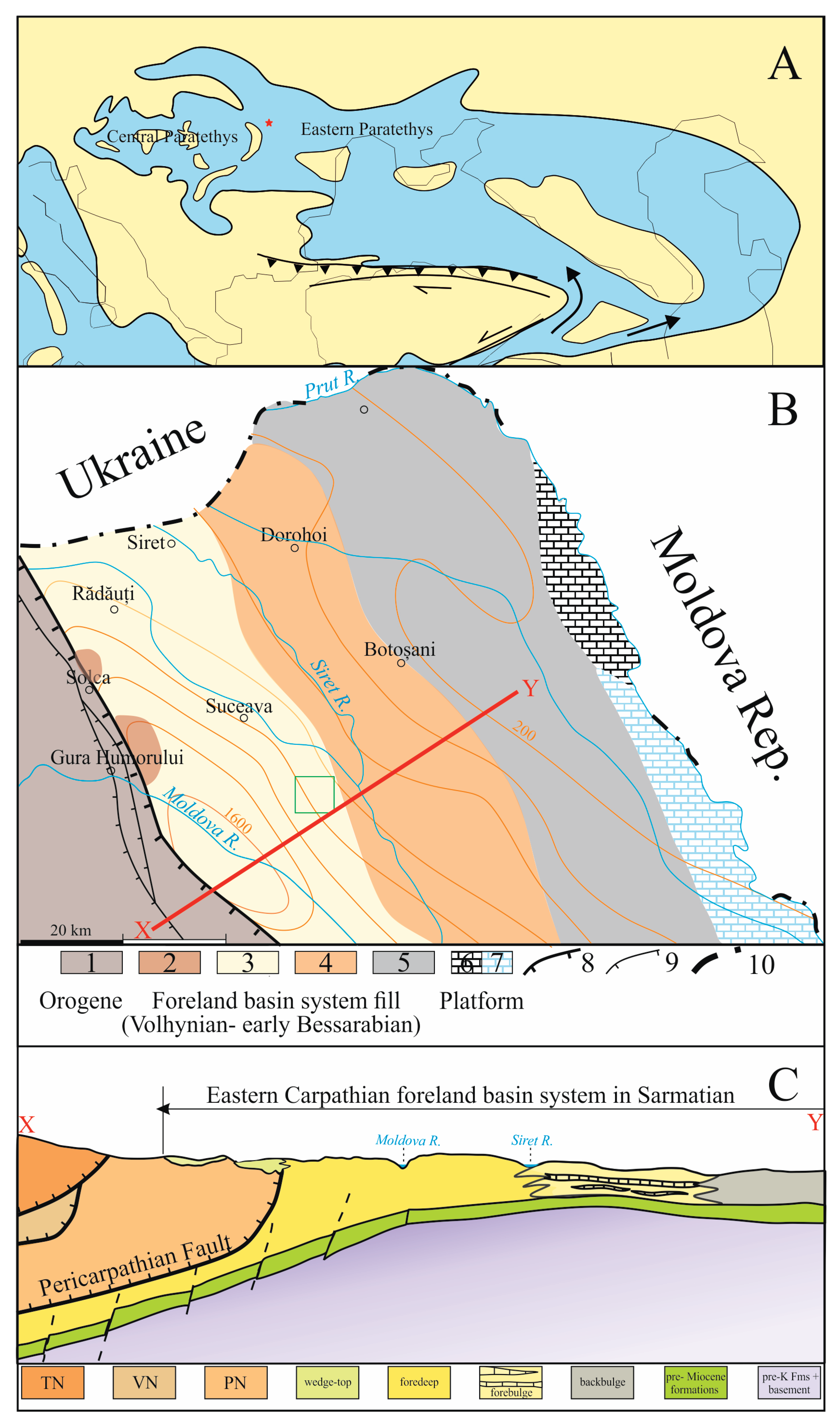
Figure 2.
Biozonation of the Volhynian – lower Bessarabian deposits exposed in the northern foreland of Eastern Carpathians (see Figure 1) based on molluscs, foraminifera, and ostracods after Ionesi [44,45] and Ionesi [28], in black, Kojumdgieva [46], in red, and Jiricek and Rija [47], in cyan.
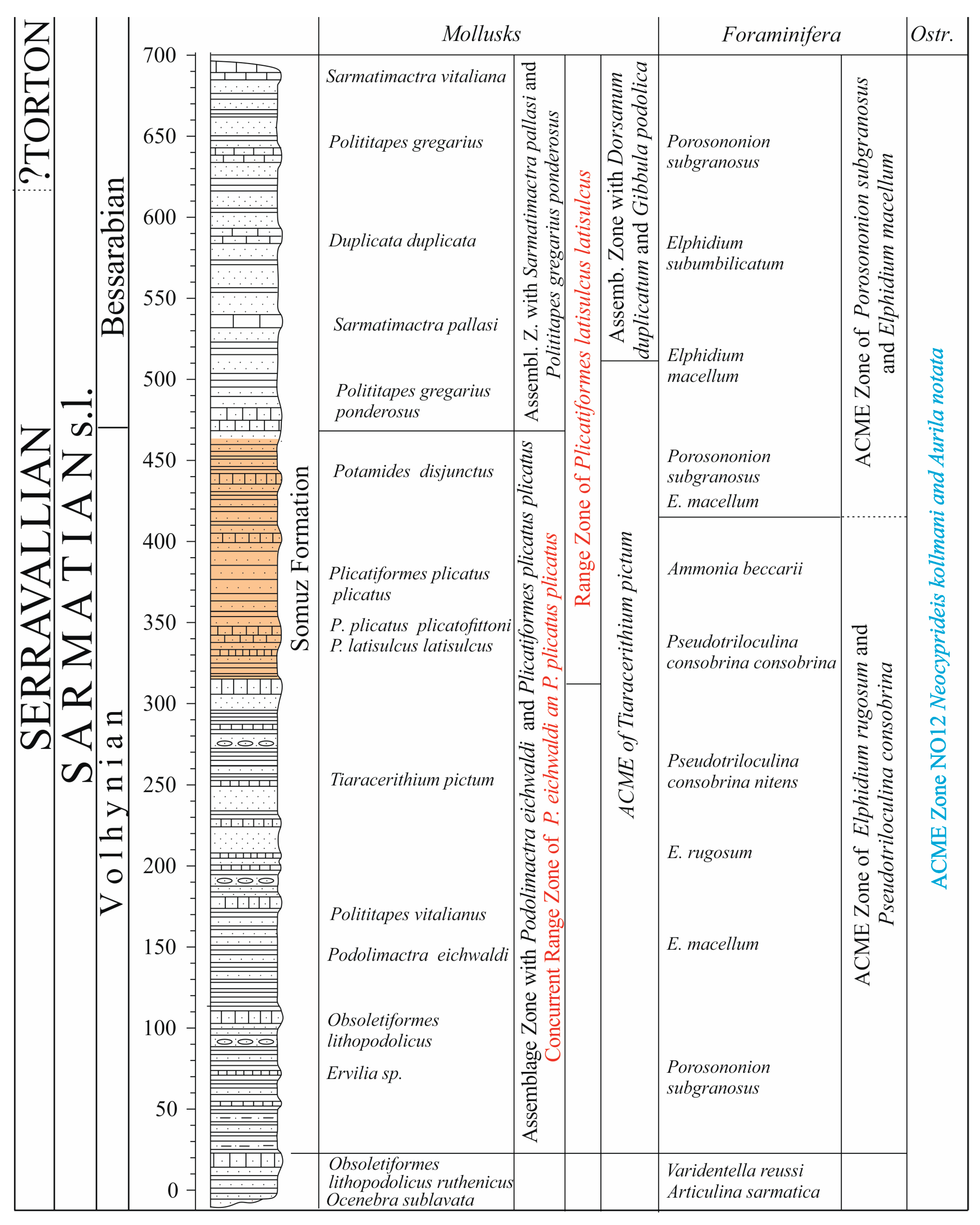
Figure 3.
Molluscs species from the studied from Șomuz Formation (the numbers in the brackets indicate the samples shown in Figure 6): 1 – Podolimactra eichwaldi (Laskarew) (365); 2,3 – Plicatiformes plicatus (Eichwald) (313; 300); 4, 5 – Polititapes tricuspis (Eichwald) (313, 300); 6, 8, 9 – Donax dentiger Eichwald (363, 365, 365); 7 – Obsoletiformes obsoletus (Eichwald) (365); 10 – Hand sample containing Plicatiformes plicatus (Eichwald) and Hydrobia sp. (313); 11 – Musculus naviculoides (Kolesnikov) (319); 12 – Ervilia sp. (274); 13,14 – Potamides disjunctus (Sowerby) (346, 281); 15,17 – Tiaracerithium pictum (Eichwald) (365, 360); 18 – Handsample with Acteocina sp. and Gibbula sp. (281); 19,20 – Duplicata duplicata (Sowerby) (281); 20 – Gibbula sulcatopodolica (Kolesnikov) (281).
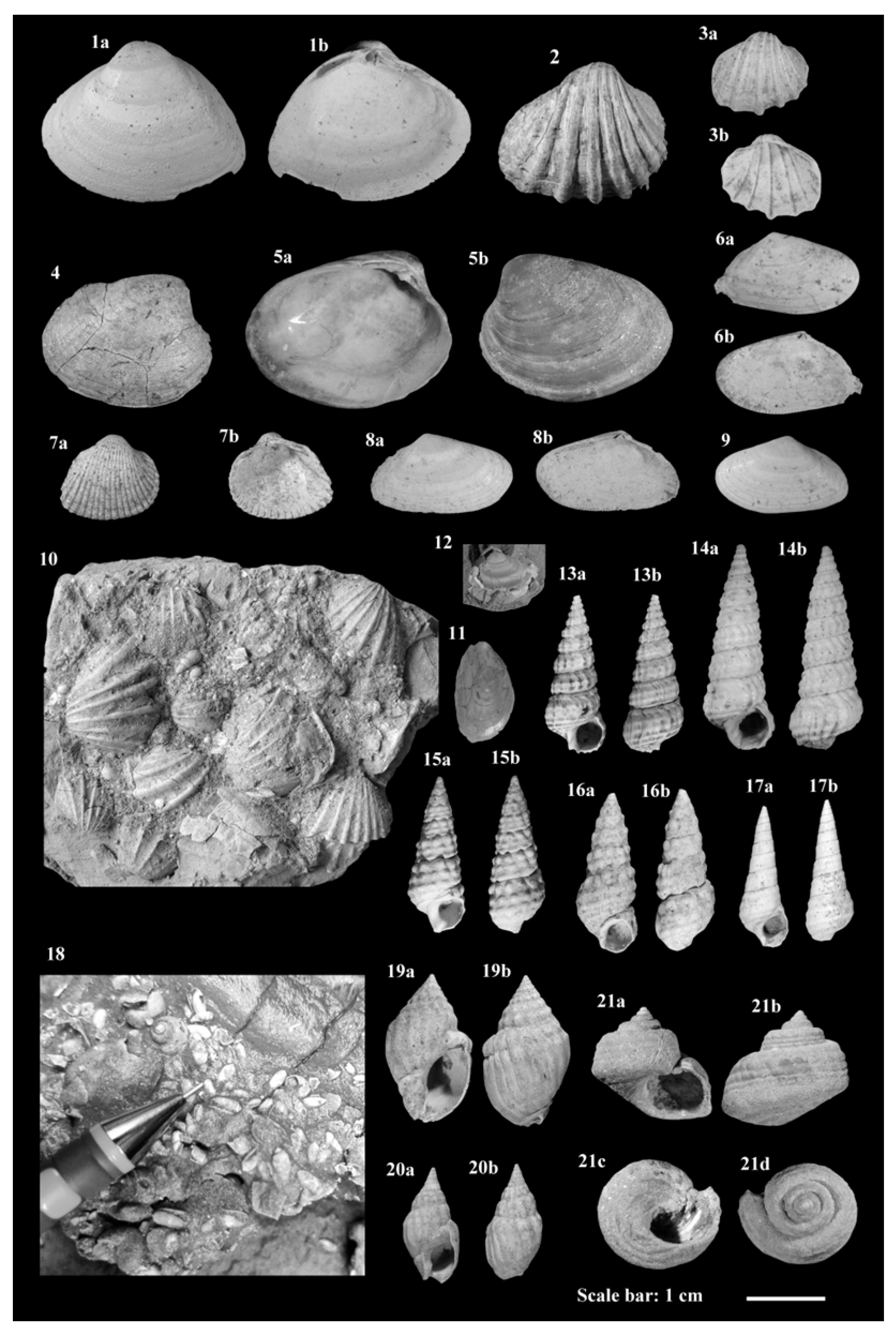
Figure 4.
SEM photos of the most representative ostracod and foraminifera taxa from the studied section (the numbers in brackets indicate samples shown in Figure 6). 1 – Cyprideis sublittoralis Pokorný (313); 2 – C. ex. gr. pannonica (Méhes) (313); 3 – C. torosa (Jones) (328); 4 – Loxoconcha minima Müller (313); 5 – L. rhomboidea (Fischer) (313); 6 – Amnicythere tenuis (Reuss) (357); 7 – Aurila mehesi (Zalányi) (332); 8 – Hemicytheria omphalodes (Reuss) (358); 9 – Pseudocandona praecox (Straub) (313); 10 – Callistocythere postvallata Pietrzeniuk (357); 11 – Xestoleberis fuscata Schneider (319); 12,13 – Elphidium hauerinum (d’Orbigny) (333); 14,15 – E. rugosum (d’Orbigny) (300, 328); 16-17 – E. macellum (Fichtel & Moll) (319); 18,19 – Porosononion subgranosus (Egger) (313); 20,21 – Ammonia beccarii (Linné) (313); 22,23 – Pseudotriloculina consobrina (d’Orbigny) (313); 24,25 – Pseudotriloculina consobrina nitens (Reuss) (332).
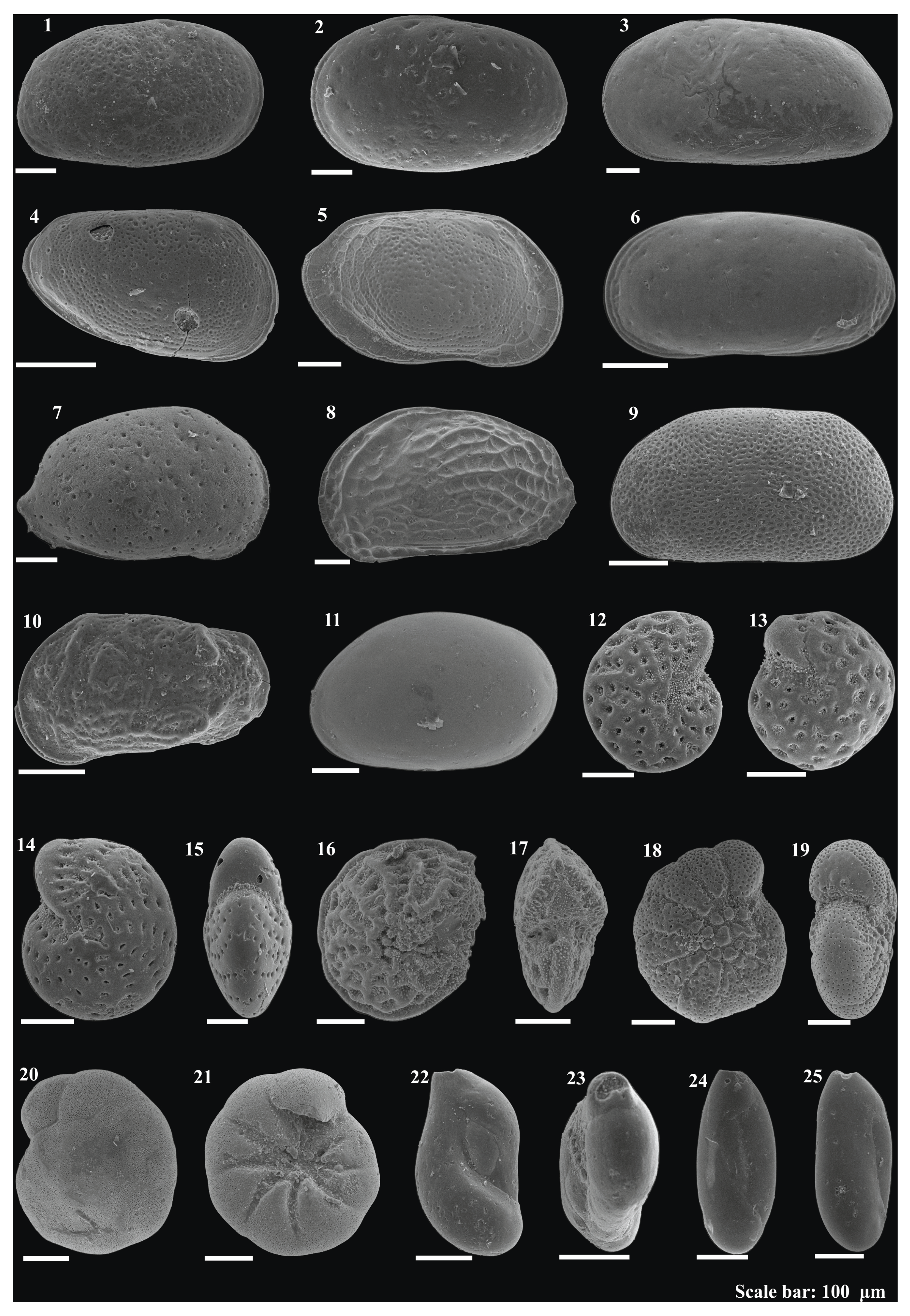
Figure 5.
High-energy, episodically affected by storms, shoreface – transition to offshore sedimentary environment reconstructed from the studied outcrops. Notice that only the three sedimentary subenvironments pictured in photos were recognized, the others being predicted according to Walther Law and on the basis of other exposures in the neighbourhood areas: O – offshore; T-O – transition zone to offshore; LSh – lower shoreface; USh – upper shoreface; FS – foreshore; BS – backshore; m – mudstones; vfs – very fine sands; fs – fine sands; ms – medium sands; cs – coarse sands. The white arrow indicates a maximum regressive surface. For the abbreviations in photos, see the text.
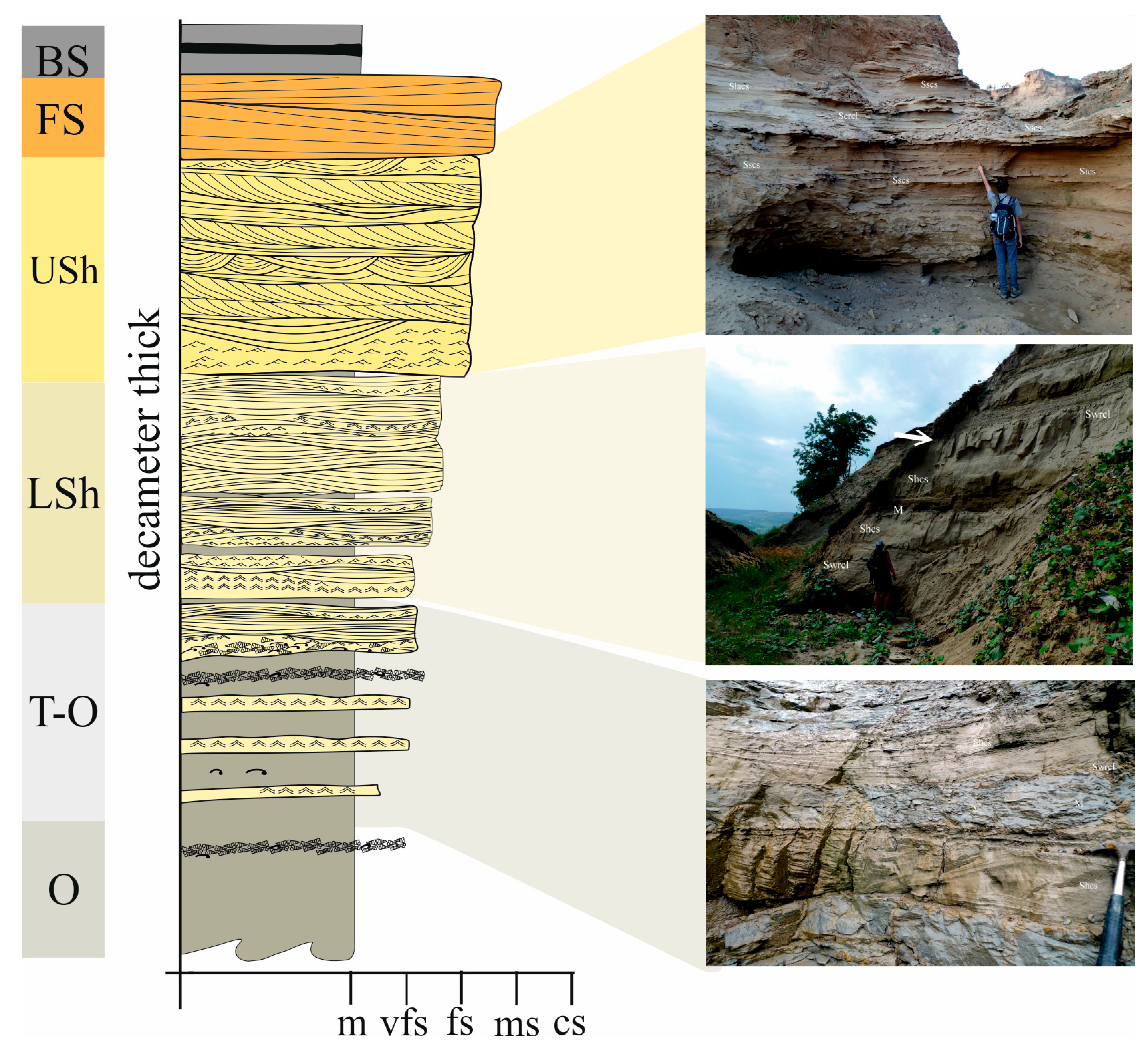
Figure 6.
The high frequency sequences (HFSs) defined in the Somuz Formation (see Figure 5 for sub-environment explanations): mrs – maximum regressive surface; mfs – maximum flooding surface: m – sandy mudstones; vfs – very fine sand; fs – fine sand; ms – medium sand; cs – coarse sand. The red dots indicate position of samples which yielded the taxa in Figure 3 and Figure 4.
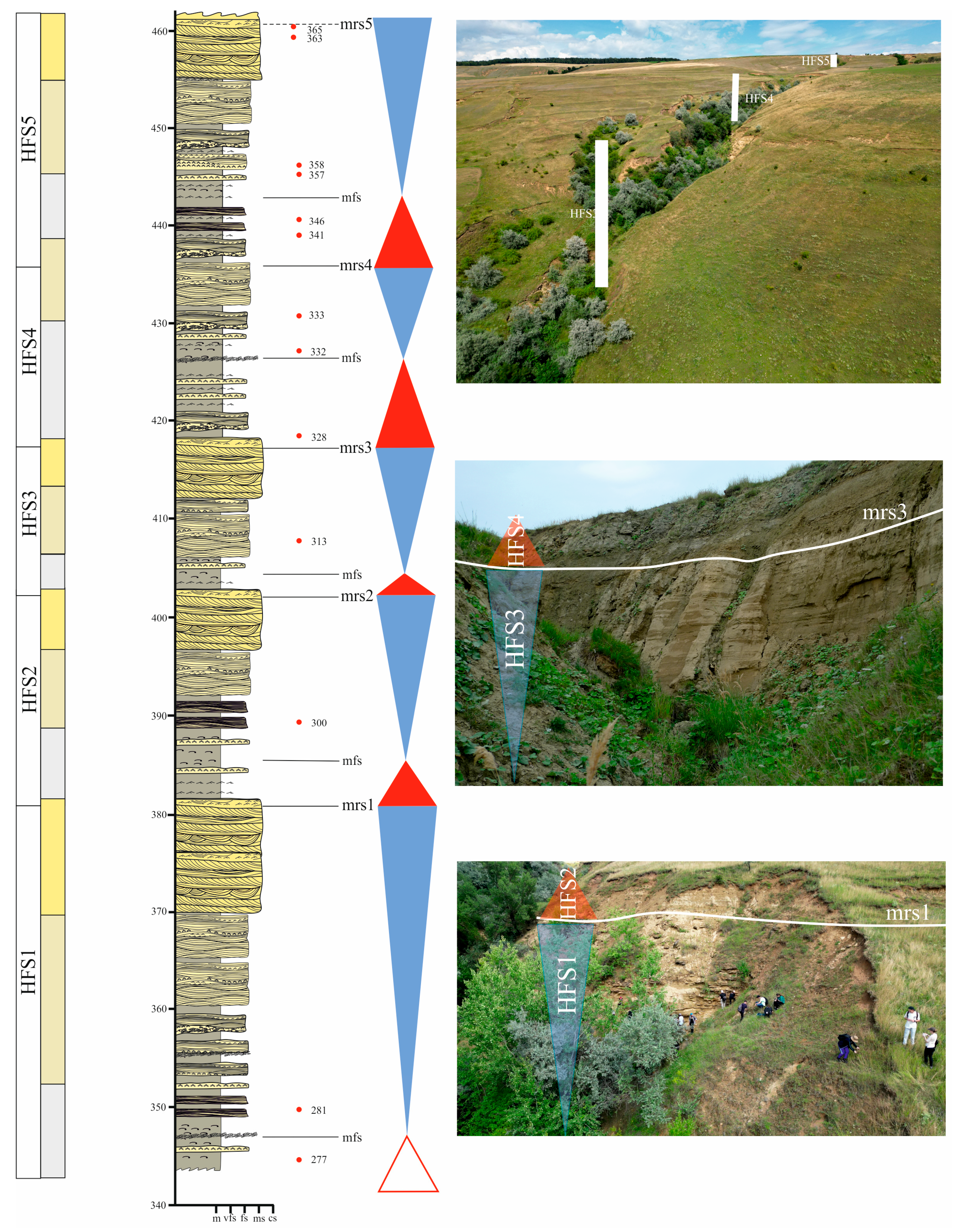
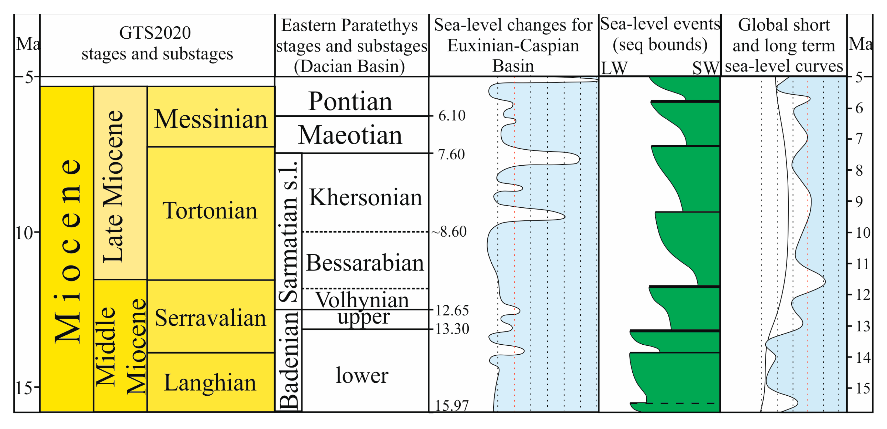
Figure 7.
Sea-level change during Volhynian (late Serravalian) in Euxianian-Caspian Basin of Eastern Paratethys (after Popov et al., 2010) [97] and at the global scale (Haq and Ogg, 2024) [98] (the dashed red lines represent the position of today-sea-level, the lines are 50 m apart, decreasing to the right). The correlation of regional stages and substages with standard ones is based on Raffi et al. (2020) [108]. LW – landward, SW – seaward.
Disclaimer/Publisher’s Note: The statements, opinions and data contained in all publications are solely those of the individual author(s) and contributor(s) and not of MDPI and/or the editor(s). MDPI and/or the editor(s) disclaim responsibility for any injury to people or property resulting from any ideas, methods, instructions or products referred to in the content. |
© 2025 by the authors. Licensee MDPI, Basel, Switzerland. This article is an open access article distributed under the terms and conditions of the Creative Commons Attribution (CC BY) license (http://creativecommons.org/licenses/by/4.0/).
Copyright: This open access article is published under a Creative Commons CC BY 4.0 license, which permit the free download, distribution, and reuse, provided that the author and preprint are cited in any reuse.


