Submitted:
21 August 2025
Posted:
22 August 2025
You are already at the latest version
Abstract
In the construction of ultra-high voltage (UHV) transformation substations, mass concrete is prone to temperature-induced cracking due to the temperature difference between internal and external environments. These cracks significantly affect the load-bearing capacity of the foundation. Therefore, accurate temperature prediction and effective temperature control are critical challenges that must be addressed. To better capture temperature fluctuations and enable real-time prediction and control, this study proposes a novel hybrid model named CPO-VMD-SSA-Transformer-GRU for predicting concrete temperature. Firstly, sine functions with different sample sizes were simulated using three models: Transformer-GRU, VMD-Transformer-GRU, and CPO-VMD-SSA-Transformer-GRU.It can be observed that the CPO-VMD-SSA-Transformer-GRU model achieves higher accuracy and faster convergence toward theoretical values, and then five performance metrics have been evaluated named Mean Absolute Error (MAE), Mean Square Error (MSE), Root Mean Square Error (RMSE), and Coefficient of Determination (R²). Furthermore, the proposed deep-optimized model was applied to predict temperature variations in mass concrete. For a single time series in the lab, the evaluation metrics for Checkpoint 1 and Checkpoint 2 were respectively 0.033736, 0.0018812, 0.0013051, 0.036127, 0.98832 and 0.016725, 0.00091304, 0.00036536, 0.019114, 0.96773, indicating corresponding reliability in predicting high-dimensional and nonlinear temperature behavior. In addition, the proposed model was extended to multi-variable time series for practical cocrete construction. The MAE, MSE, RMSE, and R² values for Checkpoint 1 were respectively 0.56293, 0.34035, 0.58339, 0.95414 and 0.85052, 0.78779, 0.88757, 0.91385. These results show improved performance compared to the single-variable model, further validating the high accuracy and reliability of the multi-variable CPO-VMD-SSA-Transformer-GRU.Therefore, the multi-variable model effectively captures fluctuation characteristics under complex conditions, obtaining accurate temperature prediction. The deep investigations provide an effective solution for temperature prediction and corresponding optimized control in real construction environments.
Keywords:
ultra-high voltage(UHV) transformation substations
; mass concrete
; during construction
; temperature series
; CPO-VMD-SSA-Transformer-GRU model
; temperature prediction
1. Introduction
In recent years, the State Grid Corporation of China (SGCC) has been actively implementing the national energy security strategy of "Four Revolutions and One Cooperation," driving the high-quality advancement of ultra-high voltage (UHV) transmission infrastructure while accelerating the development of next-generation power systems. The Sichuan-Chongqing 1000 kV UHV AC transmission project[1], commissioned in 2024, stands as a landmark demonstration of establishing a modern energy architecture in Southwest China and contributing substantively to national “carbon peaking and neutrality” objectives. Four new UHV substations along its corridor all involve in featuring massive concrete raft foundations, especially including large single-pour concrete volumes with significantly high cementitious material content[2]. This construction methodology generated substantial heat of hydration within short period, creating pronounced thermal gradients between the concrete's core and surface regions. The resultant thermal stresses precipitated widespread cracking phenomena, critically impairing the structural integrity and load-bearing performance in the foundation. It is evident that accurate temperature prediction and effective thermal control measures are critical to mitigating early-stage excessive temperatures, enhancing crack resistance, and improving construction efficiency in large-volume concrete construction[3,4]. Therefore, precise temperature prediction and timely control during the construction phase of mass concrete hold substantial engineering significance.
Current researches include theoretical analysis, experimental investigation, and numerical simulation: Liu Yang et al.[5] examined the mechanism and effectiveness of multi-admixtures in suppressing temperature rise in mass concrete; Yang Depo et al. [6] optimized cooling pipe systems based on hydration heat distribution characteristics in ultra-high-strength concrete for temperature control; Wang Qiong [7], Gao Weijie[8], and Peng Wenming[9] et al. proposed numerical methods to simulate concrete temperature after constructing, deriving temperature and stress evolution patterns during the concrete construction. It can be observed that while numerical simulation achieves relatively high computational accuracy, which requiring high-quality, dense meshes that consume substantial computational resources, resulting in low efficiency and inability to provide real-time rapid prediction. Given the limitations of conventional analytical methods including high costs, time consuming and restricted applicability, an efficient and accurate temperature prediction method is urgently proposed for mass concrete in UHV substation during the construction to solve above critical problems.
With the rapid advancement of big data and artificial intelligence technologies, data-driven machine learning approaches have attracted more attentions to solve concrete temperature prediction, providing a new opportunity for precise temperature regulation and crack propagation prevention in mass concrete construction for substation foundations of ultra-high-voltage (UHV) transmission. Xu Bailin et al.[10]pioneered a neural network model for determining the peak temperature in concrete pouring bays, employing a multi-parametric input vector comprising pouring temperature, cooling water flow rate, cooling water temperature, and ambient air temperature, with the measured maximum temperature serving as the output response. Lv Bin et al.[11]introduced an enhanced genetic algorithm to refine field temperature prediction models, enabling more robust and accurate thermal forecasting. Zhou Junjie et al.[12] used the random forest algorithm to develop a high-fidelity predictive model for the internal peak temperature of concrete pouring bays, subsequently validating its efficacy through application in a large-scale concrete dam project. Wang Kai[13] and Guo Shenggen[14] combined numerical simulations with neural network to establish an integrated temperature prediction model for mass concrete, demonstrating strong alignment between predicted trends and empirical observations. These above studies have provided base for the development of deep learning-based temperature prediction models during mass concrete construction[15,16]. Given the inherent non-stationarity and stochastic fluctuations in construction-phase temperature time-series data, advanced preprocessing techniques can be leveraged to decompose the high-dimensional, nonlinear characteristics embedded within raw time-series signals[17]. This decomposition strategy effectively circumvents the limitations associated with conventional approaches-such as inadequate feature extraction and suboptimal predictive accuracy while training and testing models on unprocessed data. Furthermore, a hybrid deep learning architecture, incorporating temporal dependencies, can be engineered to overcome the well-documented challenges of traditional neural networks, including their susceptibility to weight sensitivity and propensity for convergence to local optima. Consequently, based on the temperature time - series characteristics of typical mass concrete construction projects, the Variational Mode Decomposition (VMD) data[18] is introduced. This technique is effective in handling non-stationary signals and noise within the time series. Leveraging the self-attention mechanism of the Transformer model[19,20,21,22], rapid parallel data processing can be achieved. When combined with the Gated Recurrent Unit (GRU)[23,24], a VMD-Transformer-GRU temperature prediction model for the mass concrete construction is established. This model enables accurate modeling of complex time-series data. The self-attention mechanism of the Transformer is utilized to model the VMD to preprocess the time series, while the GRU is responsible for capturing long term dependencies within the time series. This approach effectively circumvents problems such as gradient explosion and gradient vanishing. Furthermore, to enhance the predictive performance of the VMD-Transformer-GRU (VMD-Tr-GRU) model, meta-heuristic optimization algorithms, such as the Crested Porcupine Optimizer (CPO) [25], are employed to optimize the parameters of VMD modal decomposition. This helps to better address the non- linear and multi-modal nature of the temperature time series. Additionally, the Sparrow Search Algorithm (SSA) [23] is used to optimize the hyperparameters of the model. This optimization step improves the model's convergence rate, global search ability, and prediction accuracy, thereby effectively resolving the challenges associated with hyperparameter selection in the aforementioned model.
A 1000 kV UHV power transmission and transformation as a case study, selecting temperature time-series data from the construction phase of mass concrete. Based on CPO-optimized VMD technology, the data is decomposed into sub-sequences. The multi-head attention mechanism of Transformer is employed to extract time-series, and the SSA algorithm is introduced to optimize corresponding hyperparameters, forming a CPO-VMD-SSA-Transformer-GRU (CPO-VMD-SSA-Tr-GRU) prediction model. The temperature predictions by above methods are compared for sinusoidal time-series functions by the Transformer-GRU (Tr-GRU), VMD-Tr-GRU, and CPO-VMD-SSA-Tr-GRU models demonstrates the feasibility and superiority of the CPO-VMD-SSA-Tr-GRU model for long-term temperature prediction. The model is then applied to single time-series temperature prediction in mass concrete pouring tests, with predicted values closely matching actual monitoring data, further validating its reliability. Further research on multi-variable time-series temperature prediction shows higher accuracy compared to single time-series predictions, confirming the reliability of the CPO-VMD-SSA-Tr-GRU model for deep learning of complex temperature time-series data. The above investigations provide a new approach for temperature prediction during the mass concrete construction and offer technical support for the optimization of the temperature control in different construction environments.
2. Construction of the Deeply Optimized CPO-VMD-SSA-Tr-GRU Model
2.1. CPO-optimized VMD for Time Series Data Processing
The Variational Mode Decomposition (VMD) method achieves adaptive decomposition of nonlinear and non-stationary signals by constructing a variational optimization problem to determine the center frequency of each intrinsic mode function (IMF). Compared with the Empirical Mode Decomposition (EMD) method, VMD effectively mitigates the issue of mode mixing. As for VMD decomposition for real time series, the number of decomposition modes (K) determines the number of resulting IMFs, greater K may lead to mode mixing, whereas smaller K may result in the loss of critical signal components. Meanwhile, the quadratic penalty factor α controls the spectral bandwidth of the decomposed modes. Therefore, the selection of above two parameters significantly influences the quality and accuracy of signal decomposition. To overcome the limitations associated with empirical parameter tuning, the Crested Porcupine Optimizer (CPO), a meta-heuristic algorithm inspired by the defensive behaviors of the crested porcupine including visual, auditory, olfactory, and physical attack strategies is employed to optimize the key parameters of VMD. The CPO algorithm demonstrates high computational efficiency, fast convergence and strong robustness, better addressing the non-linearity and multi-modality of the temperature time series and presenting effective extraction of temperature variation. The procedure for decomposing temperature time series based on CPO-optimized VMD (CPO-VMD) is as follows:
Construct the variational constraint model:
In which, f(t) denotes the first high-frequency component obtained from the initial decomposition; represents the impulse signal; ωk indicates the central frequency of each component; gk(t) refers to the modal component; *denotes the convolution operator.
2) Initialize the parameters and search range of the Crested Porcupine Optimizer (CPO), and set the initial number of IMF components K, the quadratic penalty factor αand the maximum number of iterations.
3) Update the population positions based on four defense strategies in the Crested Porcupine Optimizer (CPO) to effectively explore the search space .
4) Perform iterative optimization until getting the optimal number of IMF components K and the optimal quadratic penalty factorα, thereby establishing the CPO optimized VMD modal.
2.2. Transformer Network Structure
The Transformer network Encoder is an encoder-decoder model built on a self-attention machine. The encoder part is composed of multiple independent encoding layers stacked together, which consists of a multi-head self-attention mechanism and a fully connected feedforward network. Residual connections are used around the two sub-layers, and the activation values of each layer are normalized. The self-attention mechanism reduces reliance on external information and is better at capturing the internal correlations of data or features. The self-attention mechanism calculates and adjusts the weights of the samples in the input vector while embedding the influencing factors before and after the time series.
Assuming the input vector maps each input vector to three different spaces to generate the query vector, the key vector, the value vector, and linearly map them to three matrices respectively to obtain the sample generation,,:
Use the scaled dot product as the attention scoring function:
In which, are the score of the sample in each vector, is the optimization of the training gradient, Softmax is the function normalized by column.
And then, the calculations are normalized through the residual network and corresponding results are as inputs to the feedforward neural network.
The multi-head attention mechanism is formed by concatenating multiple self-attentions, each self-attention module is called a self-attention head, and each self-attention head has a different focus, such as some heads focusing on the local information of the time series and some on the global information. The multi-head attention composed of multiple self-attention heads enables each head to perform its own duties without interfering with each other and carry out complex tasks. The multi-head attention mechanism changes the original linear layer into a low dimension, then matches it through the sub-dot product attention mechanism to obtain similar functions of different patterns, and then combines the output vectors and projects them back so that the model extracts global features.
In which, .
The output vector can be calculated from two linear variations of the fully connected feedforward network:
2.3. GRU Network
The GRU(gate recurrent unit) network uses reset gates and update gates to control information transmission, selectively memorizes state information, and incorporates input information to train the model through internal recurrent units, which can better capture relationships in long time series and help reduce problems such as vanishing gradients. A typical GRU network typically propagates in the direction of sequence transport, and the hidden layer units at the moment t are
In which, is the sigmoid function, which changes the data to [0,1],which are the reset gate and the update gate respectively,,are the weights matrix, are respectively the candidate hidden layer state information and output result;is the Hadamar product, representing the product of the elements at the corresponding positions in the matrix.。
2.4. Transformer-GRU Model Structure
The temperature time series is used as the input sequence, and feature extraction and spatial relationship modeling are performed using the Transformer network. The resulting feature sequence is input into the GRU network for time series modeling and prediction to establish the Transformer-GRU model for temperature prediction,whose structure is shown in Figure 1.
(1) Input layer: Normalize the temperature time series and apply it in the model inputs. Assume the length of the data is N, and describe as.
(2) Transformer Feature extraction layer: The layer consists of position encoding, multi-head attention mechanism, and feedforward neural network. Position information is labeled for each sample of the normalized data, representing different semantic information:
In which, pos is the position of the input sequence is, i is the dimension, is the size of the vector dimension.
Use residual connections and layer normalization after the multi-head attention mechanism and feedforward neural network:
In which, LN is the normalization of the layer, are respectively the mean and variance.
(3) GRU model: The temperature series after extracting by Transformer is applied as the inputs for this layer. The layer consists of fully connected input layers and fully connected GRU level output layers. The input fully connected layer is:
Input the combined data as a newly generated feature into the GRU cell layer to obtain the GRU layer output value h.
2.5. The Sparrow Search Algorithm
The Sparrow Search Algorithm (SSA) is a swarm intelligence optimization algorithm proposed in 2020, mainly inspired by the foraging and anti-predation behaviors of sparrows. This method is not limited by the differentiability, derivability and continuity of the objective function with advantages of strong global search ability, good stability and fast convergence. The sparrow population in SSA is divided into discoverers and followers. In each iteration, two ways are applied by the discoverer to update its position.
When the discoverer does not receive a warning signal from the scout, the updated position of discoverer is as shown in Equation (11) :
In which, t is the current iteration, epoch represents the maximum number of iterations,is the random number,is the value of the jth dimension of the ith individual during the iteration t, d represents the dimension for solving the problem,andrepresent the threshold and the warning value respectively.
When the discoverer receives the warning signal, knowing that the predator is approaching, the discoverer guides all sparrows to the safe area and updates the position to equation (12) :
In which, r is a random number that follows a normal distribution, and D is a matrix where all elements are 1 describing as 1 × D. Predators with better fitness will head towards the best discoverer, whose position is updated to Equation (13) :
In which, represents the best position for the entire population, A is a matrix in which all elements are 1deccribing as 1 × d, and all elements in the matrix are 1 or -1,.The rest discoverers with less fitness who have not found food will continue to look for food near the next location, and these discoverers update their positions to equation (14) :
If the finder in the best position detects danger, it will become the scourer, and the scourer's position is updated to Equation (15) :
In which, is the random numbers represent the current fitness of the sparrow, the optimal fitness of the population, and the worst fitness respectively. And is a constant. If the scout is not in the best position, the scout will move to the best position to reduce the probability of being preyed upon, and the position is updated to equation (20) :
2.6. Construction of Deeply Optimizated VMD-Transformer-GRU Model
The temperature time series observed during the construction of mass concrete is significantly influenced by climatic conditions, admixtures, and other factors, exhibiting high-dimensional nonlinear characteristics. To accurately predict temperature variations during the construction phase, the CPO-optimized Variational Mode Decomposition (VMD) method is employed for time series preprocessing, yielding a set of intrinsic mode function (IMF) sub-series. Subsequently, the Transformer architecture, equipped with a multi-head attention mechanism, is applied to extract multidimensional features from these sub-series. Furthermore, the Gated Recurrent Unit (GRU) model, known for its strong selective memory capability and resistance to gradient explosion, is integrated to enhance the learning performance of the network. This integration results in the VMD-Transformer-GRU deep learning framework for temperature time series prediction. Given that the hybrid prediction model involves a substantial number of hyperparameters, empirically setting these parameters often leads to suboptimal performance. Therefore, it is essential to optimize these hyperparameters to improve both computational efficiency and prediction accuracy. Therefore, the Sparrow Search Algorithm (SSA) is introduced to optimize the hyperparameters of the VMD-Transformer-GRU (VMD-Tr-GRU) model, resulting in the CPO-VMD-SSA-Transformer-GRU (CPO-VMD-SSA-Tr-GRU) model. This improved model demonstrates computational efficiency and accuracy, enabling more precise prediction for mass concrete temperature behavior. The computational workflow of the CPO-VMD-SSA-Tr-GRU model is illustrated in Figure 2.
Step 1: For the acquired temperature time series of mass concrete, the Variational Mode Decomposition (VMD) process is optimized using the CPO algorithm by tuning key parameters such as the IMF component numbers K and the secondary penalty factor α. Based on these optimized parameters, the time series is decomposed into corresponding sub-sequences, which are subsequently normalized.
Step 2: The Transformer architecture is employed to extract features from the preprocessed sub-sequences, thereby capturing the nonlinear relationships between observed and predicted values. The Gated Recurrent Unit (GRU) model, which possesses selective memory capabilities, is utilized to capture temporal dependencies and dynamically adjust weights, thereby enhancing the visibility of subtle autocorrelations within the time series. The preprocessed data is then applied into the GRU model to construct a composite neural network model-VMD-Transformer-GRU (VMD-Tr-GRU) that integrates both nonlinear and temporal characteristics. The number of input and output layers is also configured accordingly.
Step 3: The Sparrow Search Algorithm (SSA) is introduced to optimize the hyperparameters of the VMD-Tr-GRU model. Key SSA parameters, including the maximum number of iterations (epoch), dimension (d), threshold (ST), and warning value R2, are initialized. The algorithm optimizes critical hyperparameters such as the initial learning rate, the number of hidden units, and the maximum training epochs. The fitness of each sparrow individual is evaluated, and the best position is updated iteratively. The corresponding hyperparameter values are imported into the VMD-Tr-GRU model to compute the fitness. Once the optimal position is reached, the algorithm terminates. Otherwise, the new position is updated as the best position for the next iteration.
Step 4: The hyperparameters obtained through SSA optimization are input into the VMD-Tr-GRU model. The performance of the resulting CPO-VMD-SSA-Tr-GRU model is evaluated using standard evaluation metrics, including Mean Absolute Error (MAE), Mean Absolute Percentage Error (MAPE), Mean Squared Error (MSE), Root Mean Squared Error (RMSE), and the coefficient of determination (R2), as defined in Equations (17) to (21).
Step 5: The optimized CPO-VMD-SSA-Tr-GRU model is applied to predict each time subsequence. The predicted values of all sub-sequences are then aggregated to reconstruct the predicted output for the complete temperature time series.
In which, is the predicted temperature of the mass concrete during the construction; is corresponding monitoring temperature of the mass concrete.
3. Verification and Assessment of the Deeply Optimized VMD-Transformer-GRU Model
A sine function was selected for analysis, where t represents time, and the time interval was set to 0.01s to construct the time series. This time series was then proportionally divided into input-output training and testing sample sequences, typically allocating 90% of the data for training and 10% for testing. An optimized VMD was applied to the time series, using an appropriate number of intrinsic mode functions (IMFs) K=5, and a quadratic penalty factor α=877. The optimized subsequences are illustrated in Figure 3
To evaluate the validity and predictive accuracy of the CPO-VMD-SSA-Tr-GRU model, several widely used performance metrics were employed such as the Mean Absolute Error (MAE), Mean Absolute Percentage Error (MAPE), Mean Squared Error (MSE), Root Mean Squared Error (RMSE), and the coefficient of determination (R2). Specifically, MAE measures the average magnitude of the absolute errors, while MAPE quantifies the average relative percentage error, offering greater robustness in error assessment. MSE and RMSE are particularly suitable for evaluating models sensitive to the magnitude of overall errors. R2, as a standard metric for assessing the predictive performance of deep learning models, better improving corresponding predictive accuracy.The optimal number of hidden units, the maximum training epochs, and the initial learning rate of the standalone Tr-GRU, VMD-Tr-GRU, and CPO-VMD-SSA-Tr-GRU models were compared and analyzed to assess the predictive performance of the proposed model. These results are summarized in Table 1 and Table 2, as well as Figure 4. Additionally, under the consideration of a Sparrow Search Algorithm (SSA) population size of 3 and 5 iterations, a comparative simulation study based on the CPO-VMD-SSA-Tr-GRU model and other models was conducted, with the results presented in Table 2 and Figure 5.The results indicate that for Tr-GRU model, the values of MAE, MAPE, MSE, RMSE, and R2 are 0.098616, 0.56336, 0.012012, 0.1096, and 0.9732, respectively. For the VMD-Tr-GRU model, the corresponding values are 0.10277, 0.7167, 0.013282, 0.11525, and 0.97037. For the VMD-SSA-Tr-GRU model, the values are 0.06747, 0.53725, 0.0053055, 0.072839, and 0.98816, respectively. The CPO-VMD-SSA-Tr-GRU model demonstrates significantly lower error values across all metrics. So, the above comparisons demonstrate that the CPO-VMD-SSA-Tr-GRU model possesses a faster convergence rate and enhanced global search capability. It is capable of effectively capturing the nonlinear characteristics inherent in long-term time series data and achieving a more precise global optimal solution. This indicates that the model can rapidly converge to the optimal solution for temperature prediction and is well-suited for simulation and forecasting tasks involving complex and large-scale temperature datasets.
Furthermore, temperature predictions were conducted using different proportions of training and testing datasets (65%, 80%, and 90% of the total data allocated to the training set). The optimal number of hidden units and the maximum training epochs under these configurations are presented in Table 2 and illustrated in Figure 5. The results indicate that the CPO-VMD-SSA-Tr-GRU model exhibits strong adaptability across varying data partitioning scenarios and achieves high training accuracy. This highlights its robust generalization capability in predicting temperature time series with strong nonlinear characteristics.
4. Study on Temperature Prediction of Mass Concrete Based on a Deeply Optimized VMD-SSA-GRU Model
4.1. Temperature Predictionwith Single Time Series for Lab Construction
4.1.1. Test Design
The testing concrete has dimensions of 1 m × 1 m × 1 m. The mix design includes Portland cement (P.O)with a compressive strength of not less than 42.5 MPa, coarse and medium sand with a fineness modulus of 2.5 or higher, continuously graded crushed stone with a particle size range of 5-31.5 mm, tap water, fly ash, and citric acid as a retarder. The detailed mix proportions are presented in Table 3, and the prepared concrete sample prior to pouring is shown in Figure 6.
4.1.2. Layout of the Cooling Pipes
The cooling water pipes are arranged in a single layer, with each layer positioned at the center of the concrete thickness (0.5 m). The flow rate is maintained at 1 m/s. The piping layout is illustrated in Figure 7, the corresponding parameters are summarized in Table 4, and the cooling water temperature is assumed to be equivalent to the environment temperature.
4.1.3. Placement of Temperature Measurement Points
The thermometer model used is SIN-RN3000, and the temperature sensor is RN3000. A total of six internal measurement points were symmetrically arranged within the concrete block, as illustrated in Figure 8. The temperature of the concrete during the water cooling process was automatically collected and recorded.
4.1.4. Temperature Time Series Prediction Based on Lab Test
To validate the reliability and superior performance of the CPO-VMD-SSA-Tr-GRU model in predicting temperature time series for mass concrete, a comparative analysis was conducted between this model and other models such as the standalone Tr-GRU and the VMD-Tr-GRU. The temperature time series for points 1 and 2 during the concrete construction in lab were used as input datasets. The selected temperature time series from the laboratory test were preprocessed using the CPO-VMD technique (Figure 9) and subsequently applied into the proposed models for prediction. The computational results are summarized in Table 5, Table 6, Table 7 and Table 8 and illustrated in Figure 10 and Figure 11. Based on these results, the predictive performance of each model was systematically compared and analyzed.
The prediction results presented in Table 5, Table 6, Table 7 and Table 8 and Figure 10 and Figure 11 indicate that the Tr-GRU and VMD-Tr-GRU models exhibit sensitivity to fluctuating data, with relatively low accuracy in capturing peak values and overall trends, presenting limitations in their nonlinear fitting capabilities. In contrast, the VMD-SSA-Tr-GRU model demonstrates significantly higher prediction accuracy across the entire fluctuation range. This improvement is primarily attributed to the Sparrow Search Algorithm (SSA), which optimizes key hyperparameters such as the number of hidden units, maximum training epochs, and initial learning rate during the model training process, thereby enhancing the overall predictive performance.
Consequently, the CPO-VMD-SSA-Tr-GRU model achieves superior prediction accuracy for the given time series. A comparative analysis of the prediction results confirms the feasibility of the hyperparameter optimization strategy employed in this model, which effectively improves both convergence speed and computational accuracy.
Based on the error analysis and prediction outcomes, the results for monitoring point 1 are as follows.For the standalone Tr-GRU model, the values of Mean Absolute Error (MAE), Mean Absolute Percentage Error (MAPE), Mean Squared Error (MSE), Root Mean Squared Error (RMSE), and the coefficient of determination (R2) are 0.26985, 0.014994, 0.074717, 0.27334, and 0.33159, respectively. For the VMD-Tr-GRU model, the corresponding values are 0.18487, 0.010216, 0.041103, 0.20274, and 0.6323. For the CPO-VMD-SSA-Tr-GRU model, the values are 0.033736, 0.0018812, 0.0013051, 0.036127, and 0.98832, respectively.For monitoring point 2, the results are as follows.For the standalone Tr-GRU model, the values are 0.11977, 0.0065454, 0.014632, 0.12096, and -0.29235. For the VMD-Tr-GRU model, the values are 0.10629, 0.0058106, 0.012472, 0.11168, and -0.10157. For the CPO-VMD-SSA-Tr-GRU model, the values are 0.016725, 0.00091304, 0.00036536, 0.019114, and 0.96773. The CPO-VMD-SSA-Tr-GRU model consistently outperforms the other models in terms of prediction accuracy, indicating that the integration of CPO for preprocessing and SSA for hyperparameter optimization significantly enhances its predictive capabilities. Furthermore, to further improve the accuracy of temperature prediction during the construction of mass concrete, it is recommended to consider the correlation between dominant temperature-influencing factors and actual temperature readings. A prediction model considering multivariate temperature series based on the CPO-VMD-SSA-Tr-GRU model can be developed to enhance both the efficiency and accuracy of temperature prediction in complex construction environments.
4.2. Field Temperature Prediction Based on Multivariate CPO-VMD-SSA-Tr-GRU Model
4.2.1. Project Overview
As for a typical new 1000kV substation, the pile raft foundation is 400 meters long in the longitudinal direction, and the concrete pouring involves 22 bins. According to the construction requirements, the hydration heat release rate and heat release variation law of various admixture combinations of cement-based materials were tested, and temperature sensors were set up for temperature monitoring, as shown in Figure 12. Based on the proposed deep learning prediction method, the temperature of mass concrete during the construction was predicted to provide technical support for the optimization of the temperature control.
Feasibility of the CPO-VMD-SSA-Tr-GRU modelSection 4.1 demonstrates the temperature prediction within a single time series. However, actual as for mass concrete during the construction, temperature fluctuations are closely influenced by multiple factors, including admixture composition, ambient temperature, and other environmental conditions. Temperature prediction with a single time series may lead to reduced prediction accuracy. To enhance the accuracy of temperature prediction, a deep learning-based model was developed for mass concrete construction. This model incorporates multi-factor cooperative control mechanisms considering typical characteristics of monitoring temperature series (Table 9). It aims to provide more accuracy during the actual construction, thereby offering a scientific support for effective formulation and optimized temperature control of mass concrete.
4.2.2. Temperature Prediction Analysis
The temperature series presented in Table 9 was decomposed into subsequences using the CPO-VMD technique, as illustrated in Figure 13. The resulting subsequences were then input into the VMD-SSA-Tr-GRU model to generate prediction results for monitoring point 1 in Chamber 1. These results are summarized in Table 10 and Table 11 and depicted in Figure 14. It can bve observed that for the CPO-VMD-SSA-Tr-GRU model, the values of Mean Absolute Error (MAE), Mean Squared Error (MSE), Root Mean Squared Error (RMSE), and the coefficient of determination (R2) are 0.56293, 0.34035, 0.58339, and 0.95414, respectively. In comparison with single-sequence prediction, the corresponding MAE, MSE, RMSE, and R2 were 3.0803, 10.04, 3.1686, and -0.35282, respectively, for one alternative model, and 3.3609, 12.063, 3.4731, and -0.62542, respectively. It can be concluded that the CPO-VMD-SSA-Tr-GRU model achieves significantly higher prediction accuracy for multi-variable temperature series, highlighting its strong generalization capability and effectiveness in capturing the characteristics of the temperature series.
5. Conclusions
A deeply optimized VMD-Tr-GRU model was developed to address the nonlinear characteristics of temperature series during the construction of mass concrete, with a focus on improving temperature prediction accuracy in complex environmental conditions. The key findings are as follows:
(1) A CPO-VMD-SSA-Transformer-GRU model was proposed for predicting temperature series during the construction of mass concrete centered around the GRU architecture. The comparisons were applied considering different training datasets to demonstrate its adaptability and robustness.
(2) A simulation study based on the sine function using the CPO-VMD-SSA-Tr-GRU model was conducted. By comparing the performance and simulation results of the standalone Tr-GRU, VMD-Tr-GRU, and CPO-VMD-SSA-Tr-GRU models, it was found that the CPO-VMD-SSA-Tr-GRU model effectively optimizes series characteristics by CPO algorithm and selects optimal hyperparameters using the SSA algorithm. This model solves the selection diffculty of the hyperparameters choice to enhance its learning and generalization capabilities and better predict complex temperature series.
(3) The CPO-VMD-SSA-Tr-GRU model was compared with the Tr-GRU and VMD-Tr-GRU models to validate its reliability and superiority in temperature prediction. The results illustrate that the proposed model exhibits stronger adaptability and better generalization ability to predict temperature of mass concrete with longer time series.
(4) After hyperparameter optimization, the CPO-VMD-SSA-Tr-GRU model demonstrates strong predictive performance and notable generalization ability for actual temperature monitoring points . For multi-variable temperature series prediction, the evaluations at checkpoint 1 are as follows: Mean Absolute Error (MAE) 0.56293; Mean Squared Error (MSE) 0.34035; Root Mean Squared Error (RMSE) 0.58339 ; coefficient of determination (R2) 0.95414. These results are significantly more accurate than those obtained from predictions considering single time series, showing that the multi-variable model can capture temperature variation more precisely and offers clear computational efficiency, further verifying its strong adaptability to high-dimensional, strongly nonlinear temperature series.
In conclusion, the CPO-VMD-SSA-Tr-GRU model is a feasible and effective solution for temperature prediction during the construction of mass concrete. It effectively captures the high-dimensional nonlinear characteristics of temperature time series, features a simple computational structure, fast convergence, strong global optimization capability, and high accuracy, providing a scientific base for both temperature prediction and the optimization of temperature control in mass concrete construction.
Author Contributions
For research articles with several authors, a short paragraph specifying their individual contributions must be provided. The following statements should be used “Conceptualization, X. L. , S. Y. and D. Y.; methodology, X. L.; software, X. L. , S. Y. and D. Y.; validation, F. Z. and X.S.; formal analysis, C. J.; investigation, L.D..; writing—original draft preparation, X. L. , S. Y. and D. Y.; writing—review and editing, L.Q. and H. L.. All authors have read and agreed to the published version of the manuscript.
Funding
This research was funded by Key project in Construction branch of Chongqing State Grid Power Company, grant number SGTYHT/24-JS-001.
Data Availability Statement
The data presented in this study are available on request from the corresponding author due to privacy reasons.
Conflicts of Interest
The authors declare no conflicts of interest.
References
- China Electric Power Development Report2024 [R]. https://www.nea.gov.cn/2024-07/19/c_1310782066.htm, Beijing, National Energy Administration Electric Power Planning and Design Institute, 2024.
- Li, L.; Wang, S.; Ma, M. Finite Element Analysis of Large-volume Concrete Temperature Field Under the Conditions of Sequence Method[J]. Construction technology 2019, 48, 89–92. [Google Scholar]
- National Standard of the People's Republic of China GB50496-2018,Code for Construction of Mass Concrete[S].Beijing, China Architecture & Building Press,2018.
- National Standard of the People's Republic of China GBT51028-2015,Technical Specification for Temperature Measurement and Control of Mass Concrete[S].Beijing, China Architecture & Building Press,2015.
- Liu Y, Chen J, Li Z. Synergistic suppression effect of multi-admixtures on temperature rise in mass concrete[J]. China Civil Engineering Journal 2022, 55, 89–97.
- Yang D, Chen R., Chang, Yang Rui,et al. Analysis of Time-Varying Temperature Effect of Hydration Heat of Ultra-High Strength Mass Concrete[J]. In-dustrial Construction (in Chinese). 2025, 55, 246–253. [CrossRef]
- WANG Qiong,CHEN ChangzheHU Zhijian,et al. Engineering measurement and numerical simulation of hydration heat temperature field of mass concrete for beam bearing platform[J]. Concrete 2020, 139–143.
- GAO Wei-jie. Simulation analysis of the temperature field and temperature control monitoring of mass concrete (raft foundation)[J]. Yunnan Institute for nationalities(Natural Sciences Edition) 2021, 30, 408–413.
- PENG Wenming. Simulation analysis of temperature stress during the construction period of concrete pouring blocks on rock foundation[J]. Water conservancy planning and design 2022, 88–93.
- XU Bailin,HUANG Yaoying,FU Xuekui,etal. Concrete Pouring Block's Highest Temperature Prediction Model andIt's Application Based on Uniform Design[J]. Water Resources and Power 2014, 32, 83–85, 90.
- LV Bin, LIYingwei,,LEIYongjun, et al. A Prediction Model for Temperature Field of Mass Concrete Based on Improved Genetic Algorithm[J]. China-foreign highways 2021, 41, 155–159.
- ZHOU Jun-jie,FAN Shi-wen,FANG Chen,et al. Internal Maximum Temperature Prediction of ConcretePouring Block Based on Random Forest Algorithm[J]. Water Resources and Power 2024, 42, 84–87.
- WANG Kai, ZHANG Yong, LIU Jianle,et al. Prediction of concrete box-girder maximum temperature gradient based on BP neural network[J]. Journal of Railway Science and Engineering 2024, 21, 837–850. [CrossRef]
- GUO Shenggen,ZHOU Shuangxi. Study on temperature evolution rule and prediction method of mass concrete under natural condition[J]. Water Resources and Hydropower Engineering 2018, 49, 188–196. [CrossRef]
- SHEN Chen-rui,TAN Chuan-shi,WANG Xing-xia, et al. Prediction of Concrete Temperature in Temperature Rising Stage forHigh Arch Dam Based on LSTM Neural Network[J]. Water Resources and Power 2022, 40, 101–104, 18.
- CEHNG Jing,KONG Chuisui,ZOU Kehui. Temperature field prediction during concrete construction period of pump and sluice project based on LSTM[J]. Advances in Science and Technology of Water Resource 2023, 43, 76–81.
- LI Zhaoxi, LIU Hongyan. Combining global and sequential patterns for multivariate time series forecasting[J]. Chinese Journal of Computers 2023, 46, 70–84.
- Wang Z, WangQ, WuT. A novel hybrid model for water quality prediction based on VMD and I-GOA optimized for LSTM[J]. Frontiers of Environmental Science &Engineering 2023, 17, 88. [CrossRef]
- GALASSI A, LIPPI M, TORRONI P. Attention in natural language processing[J]. IEEE transactions on neural networks and learning systems 2020, 32, 4291–4308. [CrossRef]
- WU H, XU J, WANG J, et al. Autoformer: Decomposition transformers with auto-correlation f-or long-term series forecasting[J]. Advances in neural information processing systems 2021, 34, 22419–22430.
- CHEN H, JIANG D, SAHLI H. Transformer encoder with multi-modal multi-head attention for continuous affect recognition[J]. IEEE Transactions on Multimedia 2020, 23, 4171–4183. [CrossRef]
- HUANg Yu, LIU Kankan, CHENG Tianxiao, et al. Intelligent Prediction Model for Deformation Induced by Excavation of Harbor Foundation Pit Based on Temporal Fusion Transformer[J]. Journal of Basic Science and Engineering, https://link.cnki.net/urlid/11.3242.TB.20250526.1418.
- LI Hongyang, GAO Bingpeng. Short-term PV power forecasting based on improved VMD and SAS-Attention-GRU[J]. Acta Energiae Solaris Sinica 2023, 44, 292–300.
- ZOU Zhi, WU Tiezhou, ZHANG Xiaoxing,et al. Short-term Load Forecast Based on Bayesian Optimized CNN-BiGRU Hybrid Neural Networks [J]. High Voltage Engineering 2022, 48, 3935–3945. [CrossRef]
- Abdel-Basset, Mohamed, Reda Mohamed, et al. Crested Porcupine Optimizer: A new nature-inspired metaheuristic[J]. Knowledge-Based Systems 284, 111257. [CrossRef]
Figure 1.
Structure of the Transformer-GRU model.
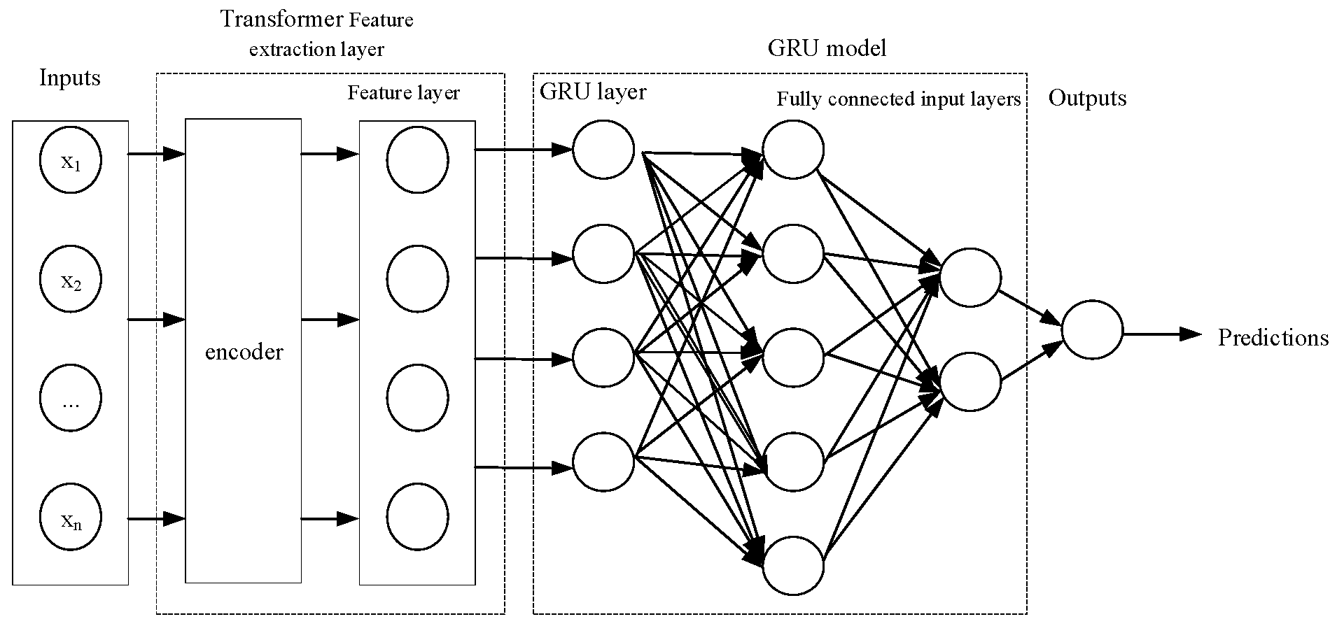
Figure 2.
Analysis diagram of the CPO-VMD-SSA-Tr-GRU model.
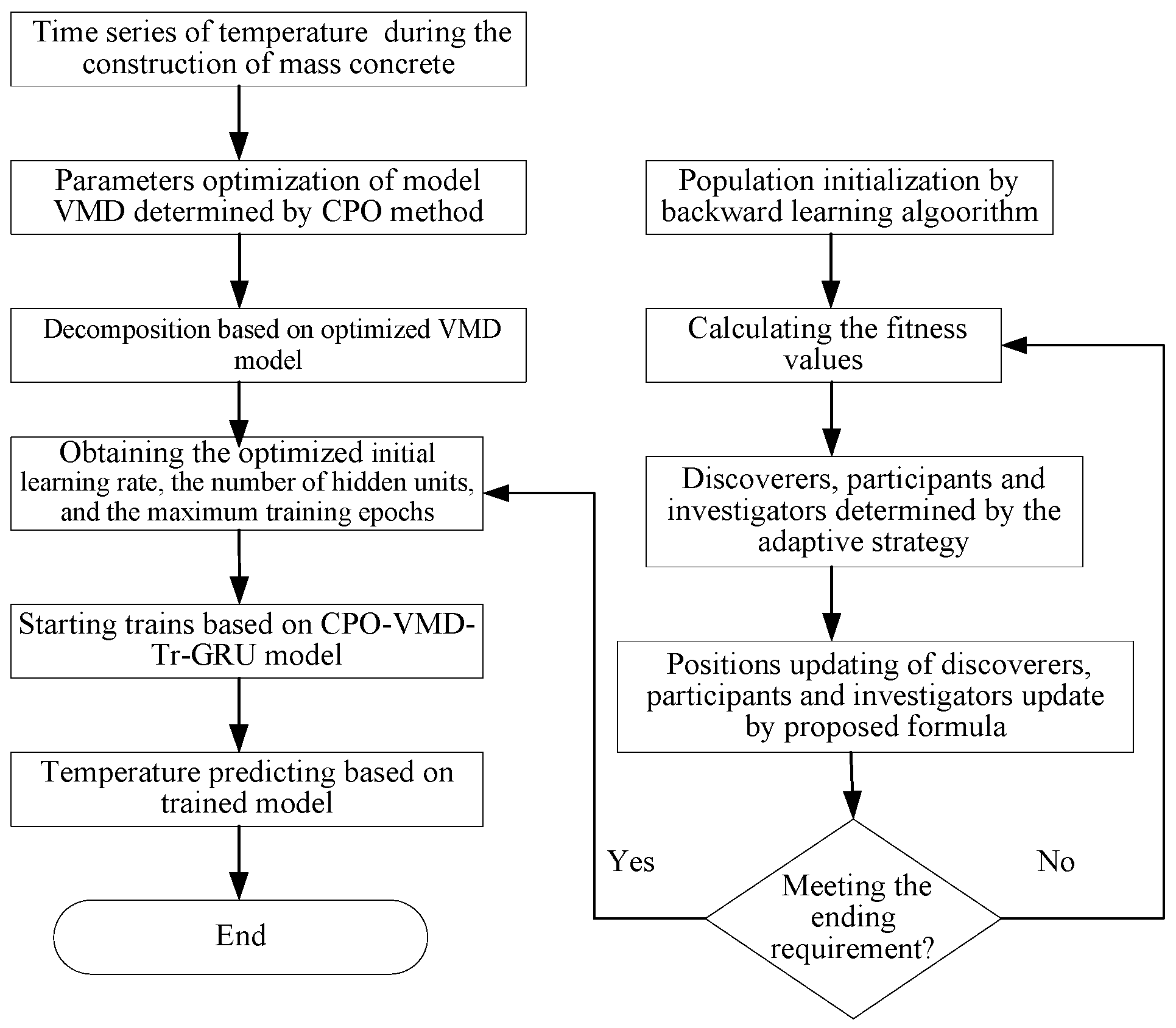
Figure 3.
Time series based on CPO-VMD decomposition.
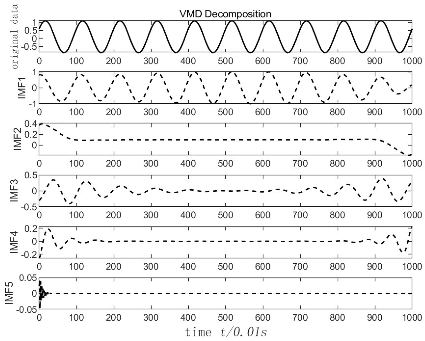
Figure 4.
Comparison of error and predicted values CPO-VMD-SSA-Tr-GRU model and other models.
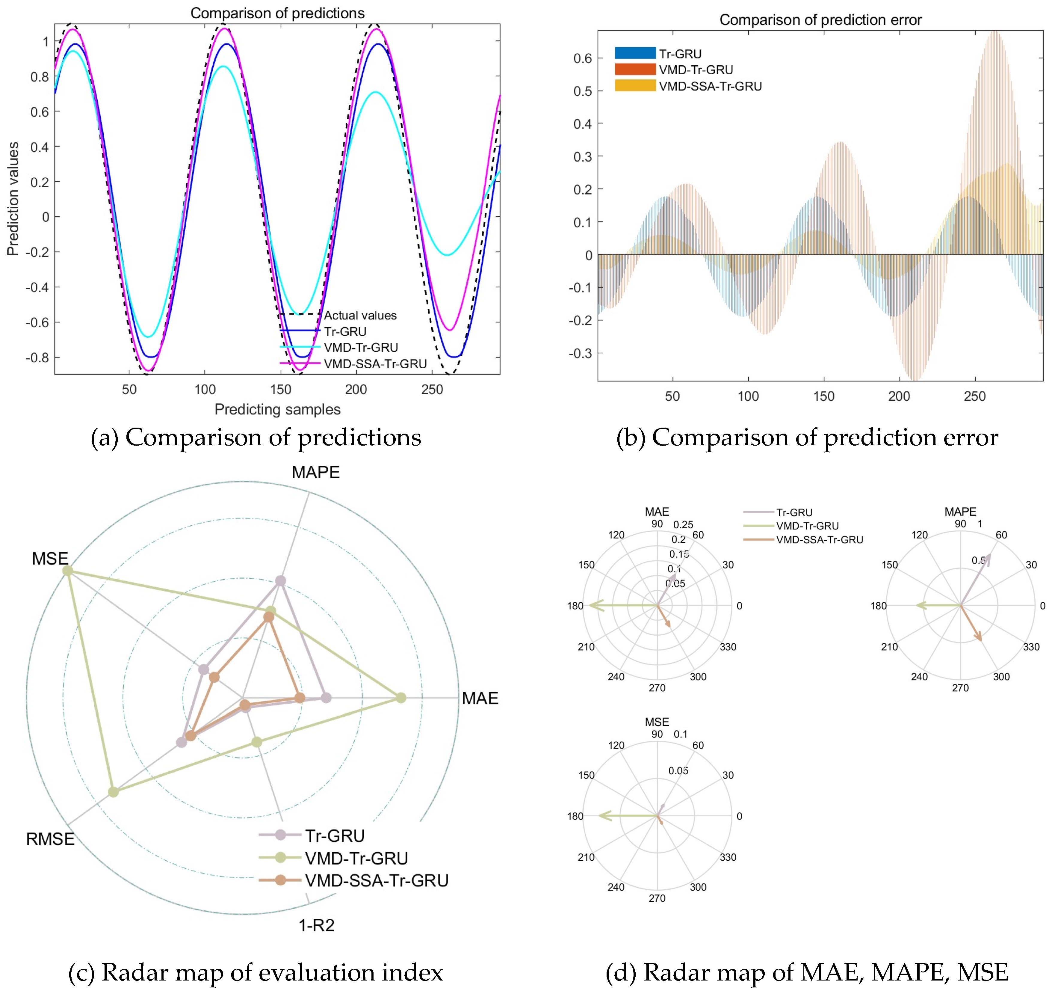
Figure 5.
Evaluation index for CPO-VMD-SSA-Tr-GRU model with different training samples and corresponding optimized parameters.
Figure 5.
Evaluation index for CPO-VMD-SSA-Tr-GRU model with different training samples and corresponding optimized parameters.
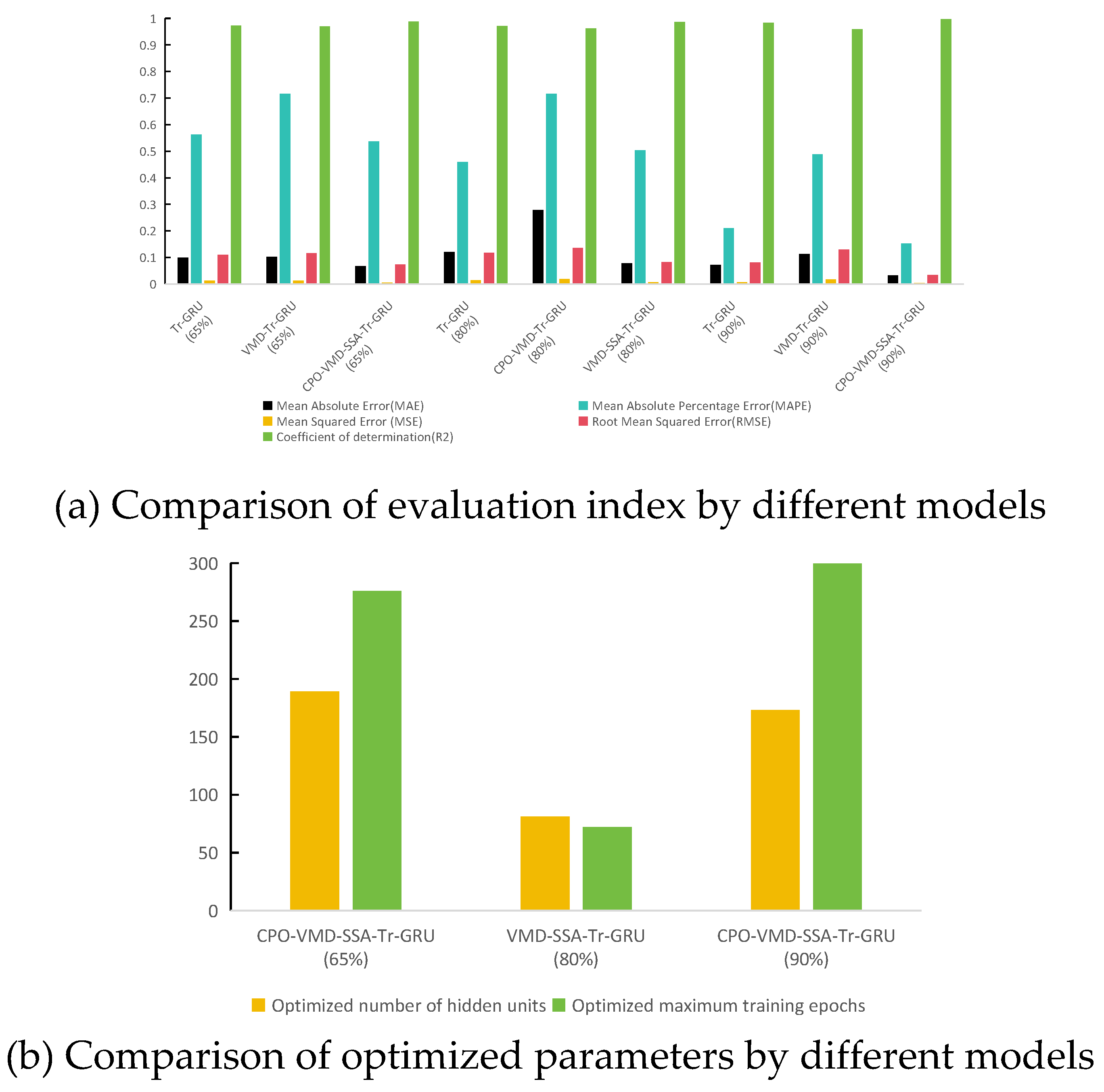
Figure 6.
The sample of mass concrete during construction.
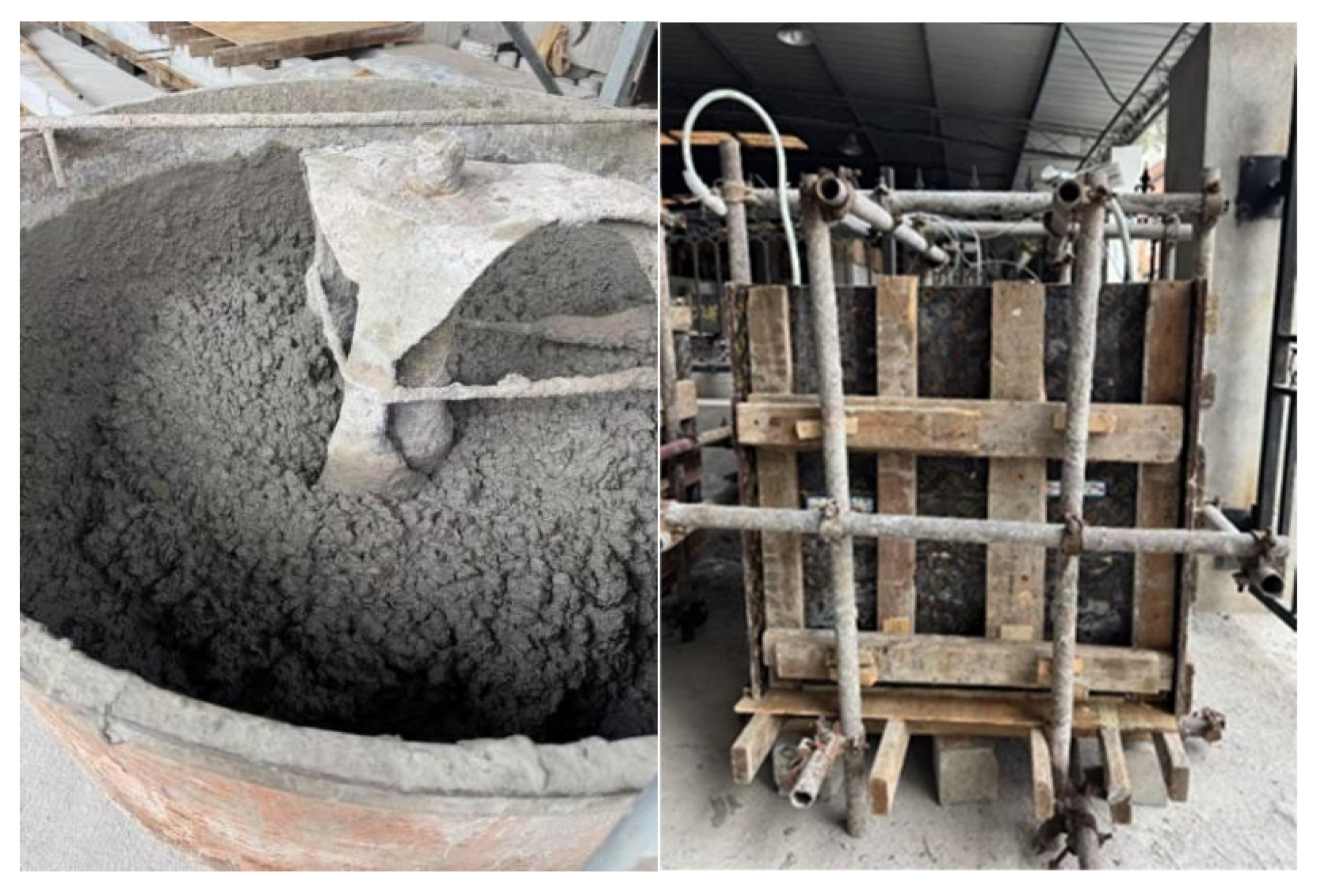
Figure 7.
The arrangement of the single-layer pipes.
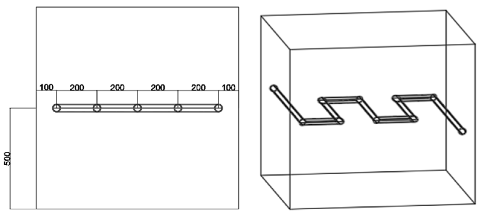
Figure 8.
The arrangement of the checkpoints.
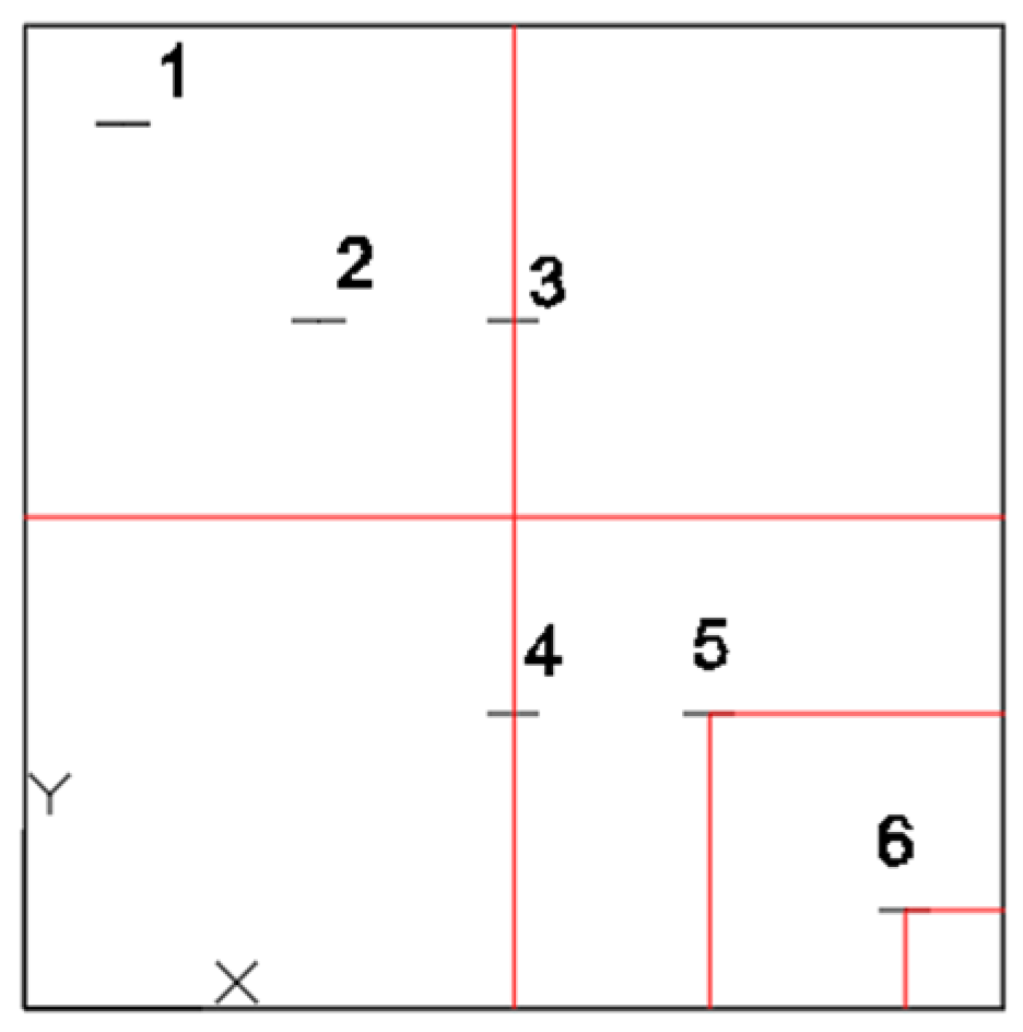
Figure 9.
Time series based on CPO-VMD decomposition.
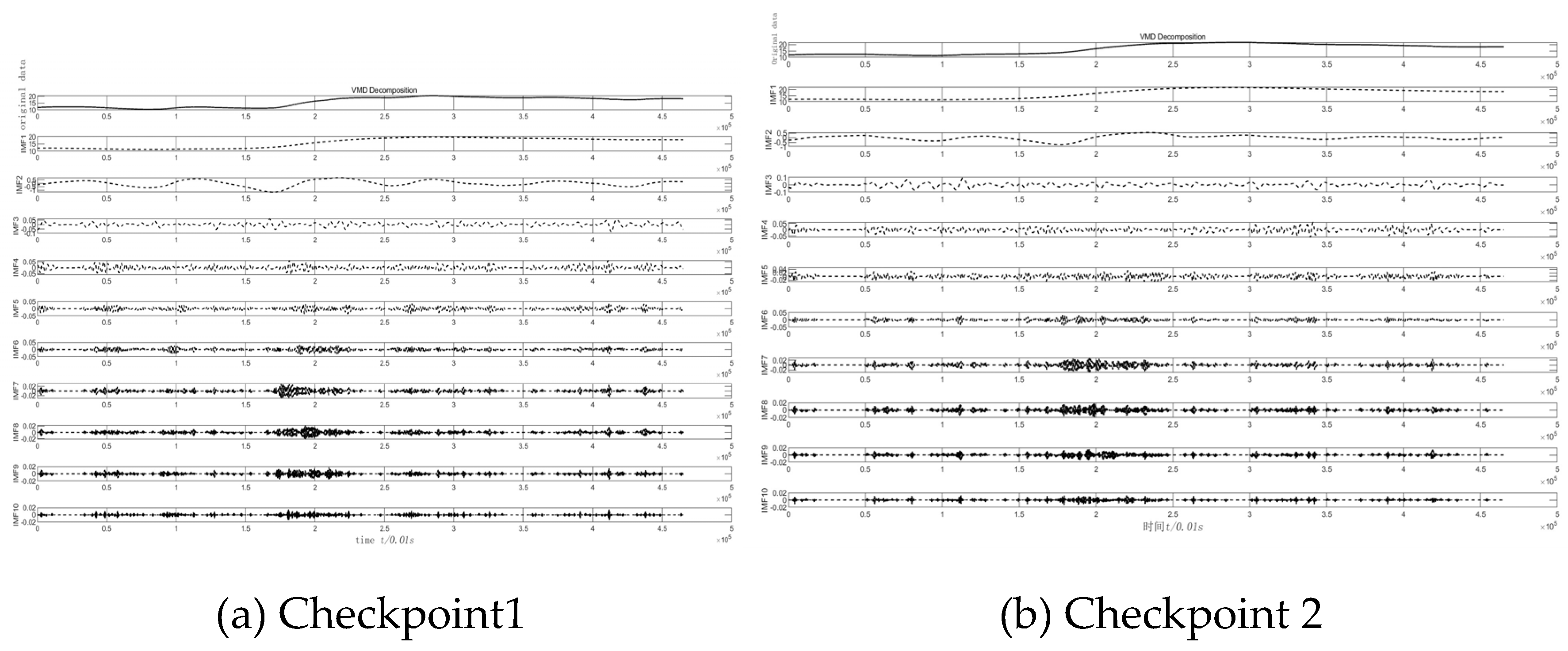
Figure 10.
Comparison of error and predicted values CPO-VMD-SSA-Tr-GRU model and other models(checkpoint 1).
Figure 10.
Comparison of error and predicted values CPO-VMD-SSA-Tr-GRU model and other models(checkpoint 1).
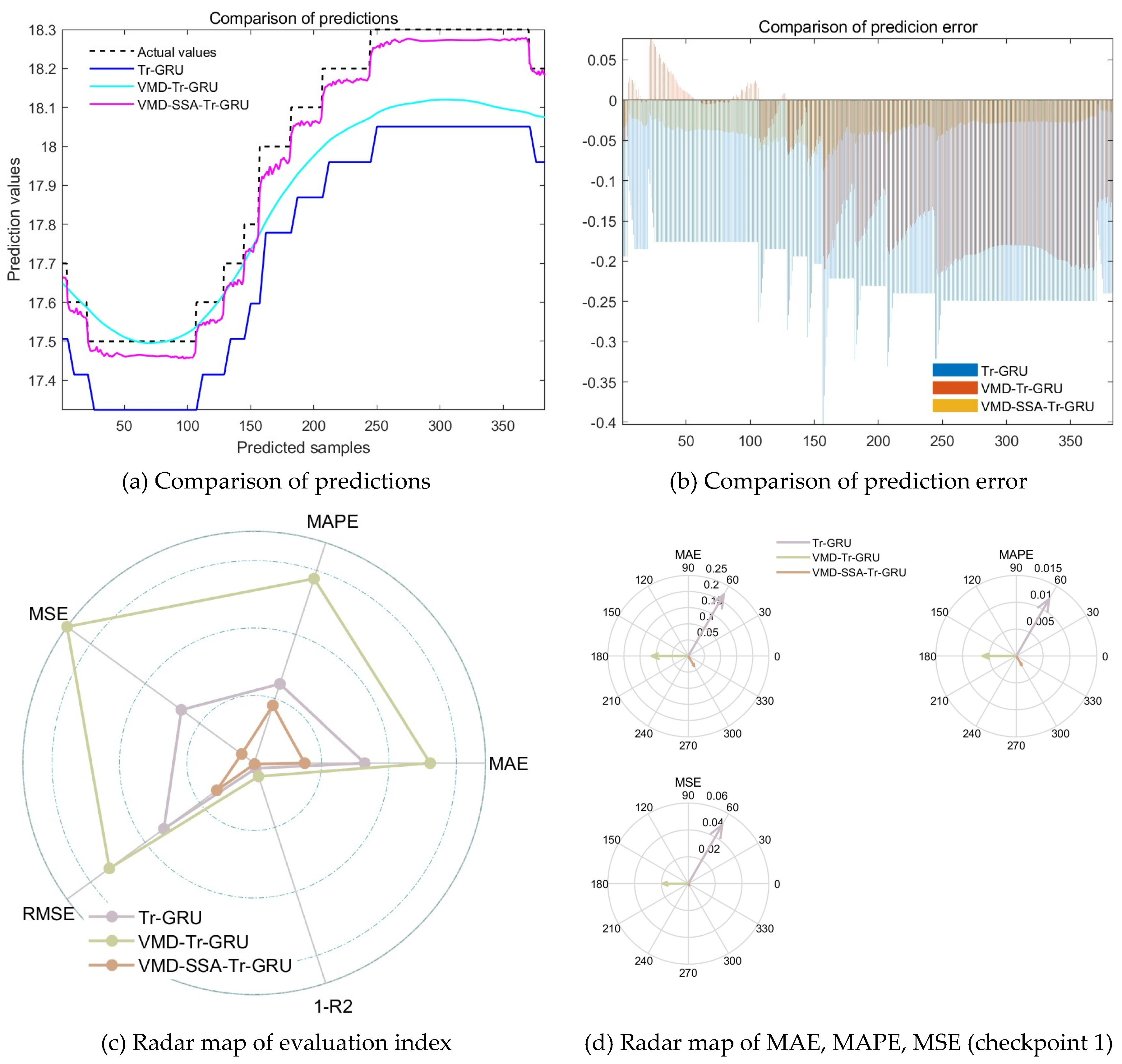
Figure 11.
Comparison of error and predicted values CPO-VMD-SSA-Tr-GRU model and other models(checkpoint 2).
Figure 11.
Comparison of error and predicted values CPO-VMD-SSA-Tr-GRU model and other models(checkpoint 2).
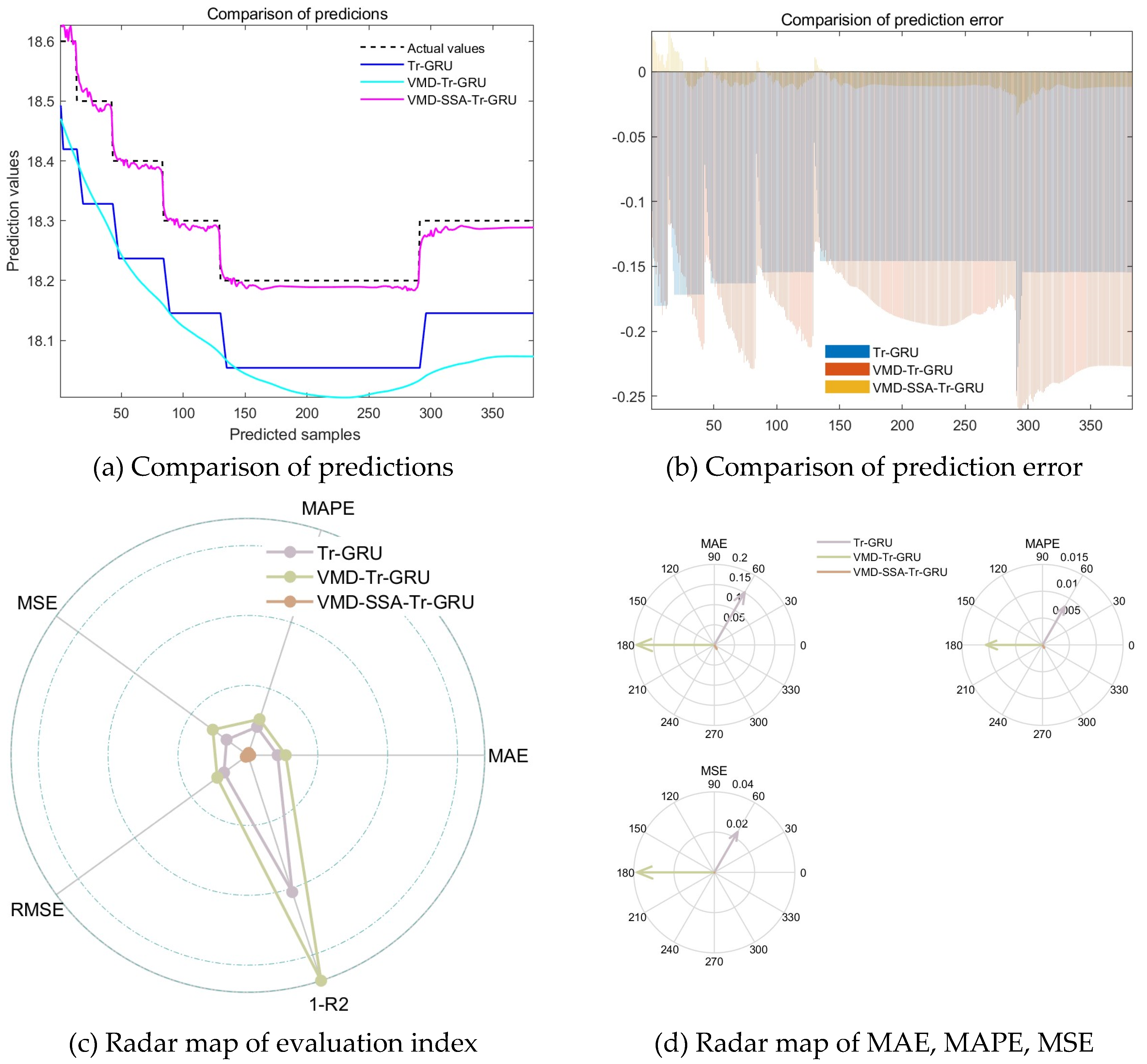
Figure 12.
Jumping construction of mass concrete and corresponding checkpoints.
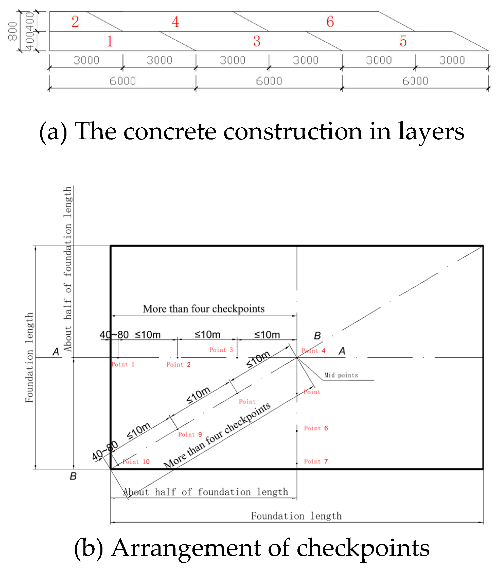
Figure 13.
Time series based on CPO-VMD decomposition.
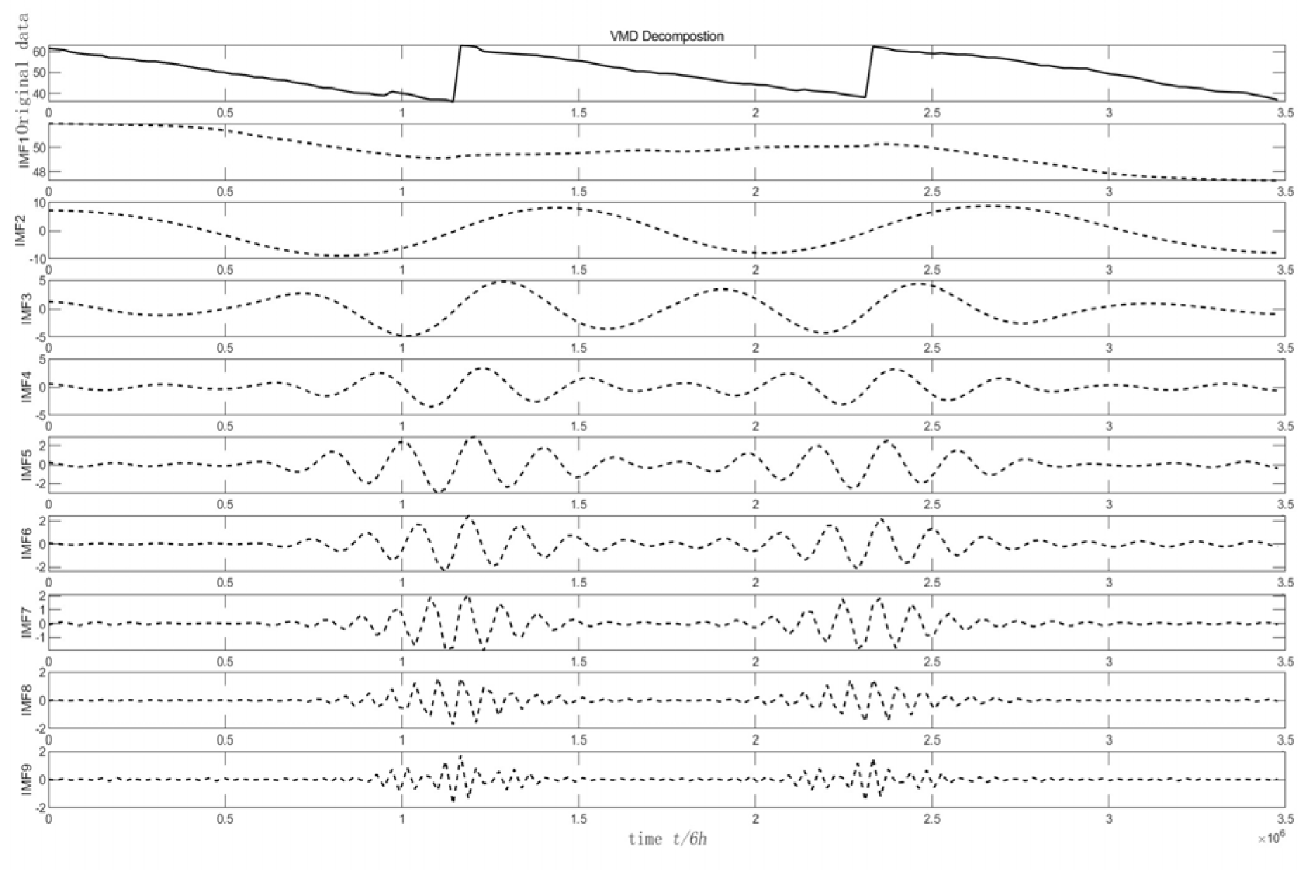
Figure 14.
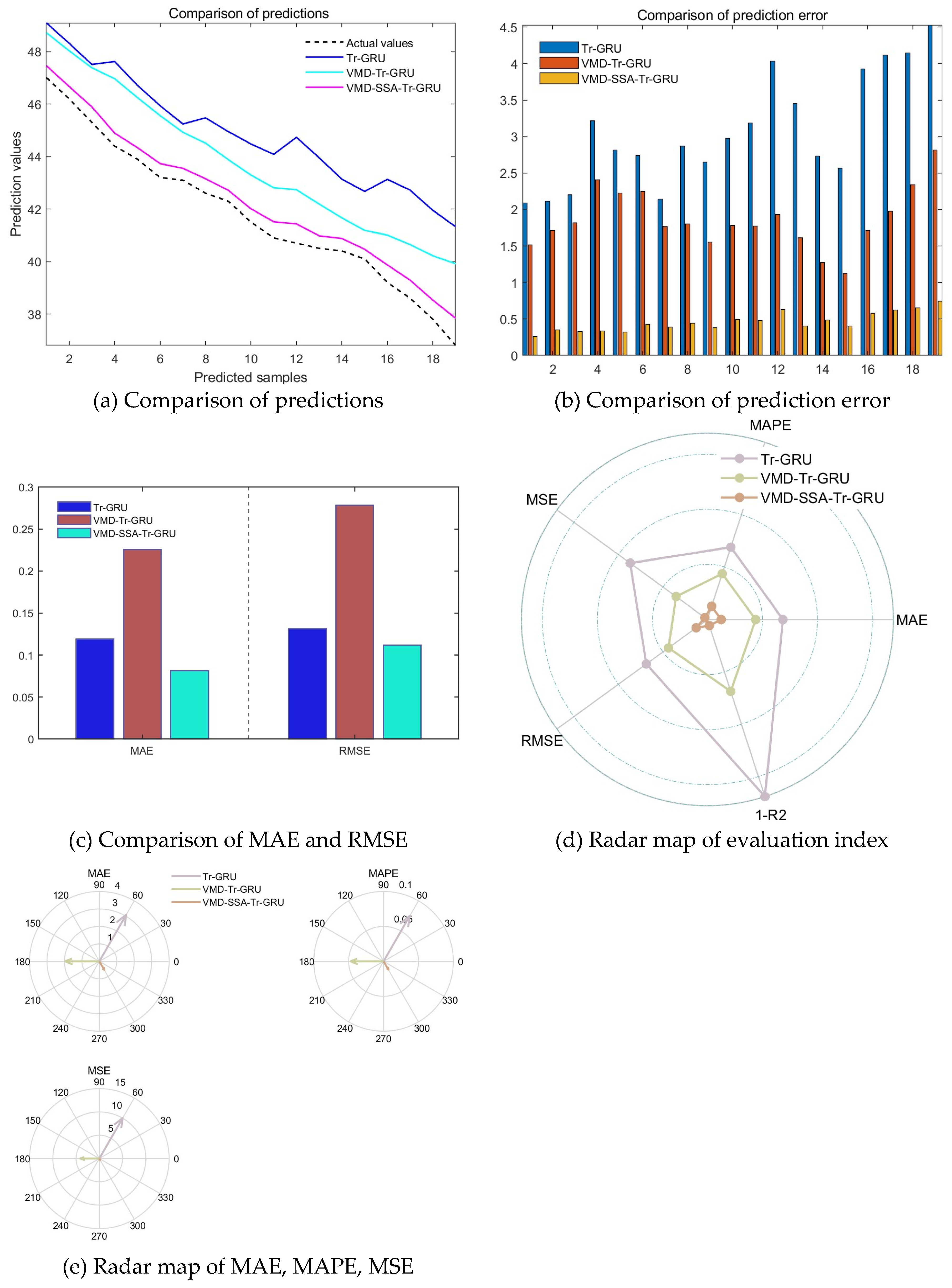

Table 1.
Evaluation index for different models and corresponding optimized parameters.
| Models type | Mean Absolute Error(MAE) | Mean Absolute Percentage Error(MAPE) | Mean Squared Error (MSE) | Root Mean Squared Error(RMSE) | Coefficient of determination(R2) | Optimized number of hidden units | Optimized maximum training epochs | Optimized initial learning rate |
| Tr-GRU(65%) | 0.098616 | 0.56336 | 0.012012 | 0.1096 | 0.9732 | |||
| VMD-Tr-GRU(65%) | 0.10277 | 0.7167 | 0.013282 | 0.11525 | 0.97037 | |||
| CPO-VMD-SSA-Tr-GRU(65%) | 0.06747 | 0.53725 | 0.005306 | 0.072839 | 0.98816 | 189 | 276 | 0.001 |
| Tr-GRU(80%) | 0.12107 | 0.45884 | 0.013775 | 0.11737 | 0.97154 | |||
| VMD-Tr-GRU(80%) | 0.27802 | 0.71633 | 0.018572 | 0.13628 | 0.96163 | |||
| CPO-VMD-SSA-Tr-GRU(80%) | 0.077425 | 0.50335 | 0.006795 | 0.08243 | 0.98596 | 81 | 72 | 0.01 |
| Tr-GRU(90%) | 0.071149 | 0.20958 | 0.006526 | 0.080781 | 0.98391 | |||
| VMD-Tr-GRU(90%) | 0.11331 | 0.48885 | 0.01676 | 0.12946 | 0.95867 | |||
| CPO-VMD-SSA-Tr-GRU(90%) | 0.032486 | 0.15236 | 0.001123 | 0.033505 | 0.99723 | 173 | 300 | 0.001 |
Table 2.
Comparison of the predicted values CPO-VMD-SSA-Tr-GRU model and other models.
| Theoretical values | Tr-GRU | VMD-Tr-GRU | CPO-VMD-SSA-Tr-GRU |
| -0.74438 | -0.63768 | -0.54035 | -0.71126 |
| -0.75424 | -0.64419 | -0.55027 | -0.72158 |
| -0.76316 | -0.64973 | -0.55933 | -0.73072 |
| -0.77113 | -0.65466 | -0.56754 | -0.7389 |
| -0.77815 | -0.65879 | -0.57487 | -0.74619 |
| ...... | |||
| -0.70032 | -0.65063 | -0.52141 | -0.68849 |
| -0.6862 | -0.64517 | -0.50911 | -0.67512 |
| -0.67121 | -0.63904 | -0.49598 | -0.66085 |
| -0.65536 | -0.63012 | -0.48203 | -0.6457 |
| -0.63867 | -0.61818 | -0.46727 | -0.62947 |
| ...... | |||
| 0.366769 | 0.254163 | 0.455529 | 0.380002 |
| 0.397657 | 0.282355 | 0.483981 | 0.410418 |
| 0.428351 | 0.31043 | 0.512218 | 0.440727 |
| 0.458819 | 0.33836 | 0.540204 | 0.471013 |
| 0.489032 | 0.366116 | 0.56791 | 0.50064 |
| ...... | |||
| 0.99653 | 0.845004 | 1.011617 | 0.96932 |
| 1.015128 | 0.863365 | 1.024764 | 0.983131 |
| 1.032921 | 0.881051 | 1.035954 | 0.995928 |
| 1.049893 | 0.898045 | 1.045545 | 1.007117 |
| 1.066025 | 0.914332 | 1.053257 | 1.016754 |
Table 3.
The ratio of the concrete specimen mix.
| Materials | Cement | Sand | Rock | Water | fly ash | citric acid |
| mix proportion /(kg/m³) | 255 | 792 | 1047 | 160 | 76.5 | 0.5 |
Table 4.
The parameters of the pipes.
| Parameters | Thermal conductivity | Density | Thermal expansion coefficient | Outer diameter | Wall thickness |
| W·( m2·K) | g·cm-3 | (1 /℃ ) | mm | mm | |
| Values | 0.15 | 1.35 | 7.0 × 10⁻⁵ | 10 | 2 |
Table 5.
Error comparison of temperature prediction with different models (checkpoint 1).
| Model (90%) | Mean Absolute Error(MAE) | Mean Absolute Percentage Error(MAPE) | Mean Squared Error (MSE) | Root Mean Squared Error(RMSE) | Coefficient of determination(R2) | ||
| Tr-GRU | 0.26985 | 0.014994 | 0.074717 | 0.27334 | 0.33159 | ||
| VMD-Tr-GRU | 0.18487 | 0.010216 | 0.041103 | 0.20274 | 0.6323 | ||
| CPO-VMD-SSA-Tr-GRU | 0.033736 | 0.0018812 | 0.001305 | 0.036127 | 0.98832 |
Table 6.
Error comparison of temperature prediction with different models(checkpoint 2).
| Model (90%) | Mean Absolute Error(MAE) | Mean Absolute Percentage Error(MAPE) | Mean Squared Error (MSE) | Root Mean Squared Error(RMSE) | Coefficient of determination(R2) | ||
| Tr-GRU | 0.11977 | 0.0065454 | 0.014632 | 0.12096 | -0.29235 | ||
| VMD-Tr-GRU | 0.10629 | 0.0058106 | 0.012472 | 0.11168 | -0.10157 | ||
| CPO-VMD-SSA-Tr-GRU | 0.016725 | 0.00091304 | 0.000365 | 0.019114 | 0.96773 |
Table 7.
Comparison of the predicted values CPO-VMD-SSA-Tr-GRU model and other models(checkpoint 1).
Table 7.
Comparison of the predicted values CPO-VMD-SSA-Tr-GRU model and other models(checkpoint 1).
| Temperature in checkpoint 1 | Tr-GRU | VMD-Tr-GRU | CPO-VMD-SSA-Tr-GRU |
| 17.7 | 17.509176 | 17.53813 | 17.702385 |
| 17.7 | 17.509176 | 17.535011 | 17.700686 |
| 17.7 | 17.509176 | 17.531834 | 17.703773 |
| 17.7 | 17.509176 | 17.528616 | 17.69643 |
| 17.6 | 17.509176 | 17.525337 | 17.640261 |
| ....... | |||
| 17.5 | 17.326246 | 17.415298 | 17.495182 |
| 17.5 | 17.326246 | 17.417297 | 17.496754 |
| 17.5 | 17.326246 | 17.419388 | 17.497347 |
| 17.5 | 17.326246 | 17.421614 | 17.497026 |
| 17.5 | 17.326246 | 17.424023 | 17.502207 |
| 17.5 | 17.326246 | 17.426636 | 17.509899 |
| ....... | |||
| 18 | 17.600578 | 17.667452 | 17.918709 |
| 18 | 17.637152 | 17.673679 | 17.94673 |
| 18 | 17.673702 | 17.68005 | 17.960423 |
| 18 | 17.710236 | 17.686457 | 17.953716 |
| 18 | 17.74675 | 17.692862 | 17.963177 |
| ....... | |||
| 18.2 | 17.965757 | 17.969032 | 18.217176 |
| 18.2 | 17.965757 | 17.968611 | 18.224201 |
| 18.2 | 17.965757 | 17.968224 | 18.231836 |
| 18.2 | 17.965757 | 17.967867 | 18.224049 |
| 18.2 | 17.965757 | 17.967585 | 18.219481 |
Table 8.
Comparison of the predicted values CPO-VMD-SSA-Tr-GRU model and other models(checkpoint 2).
Table 8.
Comparison of the predicted values CPO-VMD-SSA-Tr-GRU model and other models(checkpoint 2).
| Temperature in checkpoint 2 | Tr-GRU | VMD-Tr-GRU | CPO-VMD-SSA-Tr-GRU |
| 18.6 | 18.438955 | 18.591953 | 18.655531 |
| 18.6 | 18.402805 | 18.585485 | 18.653751 |
| 18.6 | 18.366646 | 18.579208 | 18.656033 |
| 18.6 | 18.366646 | 18.573275 | 18.65411 |
| 18.6 | 18.366646 | 18.567556 | 18.636728 |
| ....... | |||
| 18.2 | 18.095301 | 18.193825 | 18.254673 |
| 18.2 | 18.077196 | 18.191532 | 18.242689 |
| 18.2 | 18.059097 | 18.189159 | 18.235815 |
| 18.2 | 18.040998 | 18.186775 | 18.23225 |
| 18.2 | 18.0229 | 18.184435 | 18.2293 |
| ....... | |||
| 18.3 | 18.095301 | 18.187534 | 18.315294 |
| 18.3 | 18.095301 | 18.187517 | 18.315332 |
| 18.3 | 18.095301 | 18.187502 | 18.315245 |
| 18.3 | 18.095301 | 18.18749 | 18.315292 |
| 18.3 | 18.095301 | 18.187479 | 18.315359 |
Table 9.
Training and testing datasets(checkpoint 1).
| No. | Airtemperature | Temperature in checkpoint 1 |
| 1 | 27 | 61.5 |
| 2 | 29 | 61.2 |
| 3 | 35 | 60.8 |
| 4 | 30 | 59.7 |
| 5 | 25 | 59.1 |
| 6 | 24 | 58.6 |
| 7 | 33 | 58.3 |
| 8 | 26 | 58.1 |
| 9 | 24.5 | 57 |
| 10 | 23.5 | 56.9 |
| 11 | 33 | 56.5 |
| 12 | 24 | 56.2 |
| ....... | ||
| 155 | 29 | 40.7 |
| 156 | 23.5 | 40.5 |
| 157 | 21 | 40.4 |
| 158 | 20.5 | 40.1 |
| 159 | 26 | 39.2 |
| 160 | 23 | 38.6 |
| 161 | 19.5 | 37.8 |
| 162 | 19 | 36.8 |
Table 10.
Error comparison of temperature prediction with different models(checkpoint 1).
| Model (90%) | Mean Absolute Error(MAE) | Mean Squared Error (MSE) | Root Mean Squared Error(RMSE) | Coefficient of determination(R2) |
| Tr-GRU | 3.0803 | 10.04 | 3.1686 | -0.35282 |
| VMD-Tr-GRU | 1.9667 | 4.0716 | 2.0178 | 0.45136 |
| CPO-VMD-SSA-Tr-GRU | 0.56293 | 0.34035 | 0.58339 | 0.95414 |
Table 11.
Comparison of the predicted values CPO-VMD-SSA-Tr-GRU model and other models(checkpoint 1).
Table 11.
Comparison of the predicted values CPO-VMD-SSA-Tr-GRU model and other models(checkpoint 1).
| Actual temperature in checkpoint 1 | Tr-GRU | VMD-Tr-GRU | CPO-VMD-SSA-Tr-GRU |
| 47 | 48.998734 | 48.496426 | 47.413113 |
| 46.2 | 48.129364 | 47.932735 | 46.654602 |
| 45.3 | 47.373768 | 47.168629 | 45.828285 |
| 44.4 | 47.313866 | 46.59811 | 44.816147 |
| 43.9 | 46.617676 | 46.036911 | 44.310432 |
| 43.2 | 45.771885 | 45.418903 | 43.722919 |
| 43.1 | 45.075943 | 44.689621 | 43.50808 |
| 42.6 | 45.1549 | 44.154358 | 43.091953 |
| 42.3 | 44.761082 | 43.633194 | 42.700665 |
| 41.5 | 44.24445 | 43.097313 | 42.002522 |
| 40.9 | 43.835213 | 42.524963 | 41.471081 |
| 40.7 | 44.286972 | 42.286591 | 41.33123 |
| 40.5 | 43.759117 | 41.922653 | 41.030804 |
| 40.4 | 42.908455 | 41.520748 | 40.916813 |
| 40.1 | 42.51244 | 40.93829 | 40.453896 |
| 39.2 | 42.76593 | 40.625797 | 39.809101 |
| 38.6 | 42.542824 | 40.3825 | 39.277225 |
| 37.8 | 41.927334 | 40.073124 | 38.56871 |
| 36.8 | 41.40247 | 39.710876 | 37.821724 |
Disclaimer/Publisher’s Note: The statements, opinions and data contained in all publications are solely those of the individual author(s) and contributor(s) and not of MDPI and/or the editor(s). MDPI and/or the editor(s) disclaim responsibility for any injury to people or property resulting from any ideas, methods, instructions or products referred to in the content. |
© 2025 by the authors. Licensee MDPI, Basel, Switzerland. This article is an open access article distributed under the terms and conditions of the Creative Commons Attribution (CC BY) license (http://creativecommons.org/licenses/by/4.0/).
Copyright: This open access article is published under a Creative Commons CC BY 4.0 license, which permit the free download, distribution, and reuse, provided that the author and preprint are cited in any reuse.


