
Submitted:
06 April 2025
Posted:
08 April 2025
You are already at the latest version
Abstract
The incorporation of waste ground glass powder (GGP) as a partial replacement in cement offers significant environmental benefits, such as reduction in CO2 emission from cement manufacturing and decrease in the use of colossal landfill space. However, concrete is a heterogeneous material and the prediction of its accurate compressive strength is challenging due to the inclusion of several nonlinear parameters. This paper explores the utilization of different machine learning (ML) algorithm; Linear Regression (LR), Elastic Net regression (ENR), K-nearest Neighbor Regressor (KNN), Decision Tree Regressor (DT), Random Forest Regressor (RF), and Support Vector Machine (SVM). A total of 188 sets of pertinent mix design experimental data are collected to train and test the MLalgorithms. Concrete mix components such as cement content, coarse and fine aggregates, water-cement ratio (W/C) ratio, various GGP chemical properties, and curing time are set as input data (X) while the compressive strength is set as the output data (Y). The hyperparameter tuning is carried out to optimize the ML models, and the results are compared with the help of the coefficient of determination (R2) and root-mean-square error (RMSE). Among the algorithms used, SVM demonstrates the highest accuracy and predictive capability among all models with R2 value of 0.95 and RSME of 3.40 MPa. Additionally, all the models exhibit R2 value higher than 0.8, suggesting ML models provide highly accurate and cost-effective means for evaluating and optimizing the compressive strength of GGP concrete.
Keywords:
waste glass
; recycled glass
; glass powder
; cement replacement
; sustainable concrete
; compressive strength
; machine learning
; artificial intelligence
; prediction
; algorithm
1. Introduction
Concrete is a widely used construction material in the world due to its high mechanical strength in compression and economic extraction of raw materials [1,2,3,4,5,6]. However, the production of the primary ingredient in concrete, cement, uses significant industrial energy and emits a huge amount of carbon dioxide () in the world [7]. To reduce the environmental impact associated with the carbon emission, over the centuries, construction industry has been implementing various supplementary cementitious materials (SCM’s) such as fly ash (FA), ground granulated blast slag (GGBS), rice husk ash (RHA), ground glass powder (GGP), silica fume (SF), etc. as a partial replacement of cement [8]. Studies have demonstrated a considerable enhancement in the mechanical and durability properties of concrete with the inclusion of different SCMS [9,10,11,12,13]. This enhancement is a result of the pozzolanic reaction between from SCMs and cement hydration by product calcium hydroxide Ca(OH)2 [14]. The pozzolanic reaction forms an additional binding material; calcium silicate hydrate (C-S-H) gel that fills the voids and provides more strength to the concrete [15]. Among the available SCMs, GGP derived from waste glass can be a suitable alternative to the commonly used SCM, FA, due to its low recycling rates in major countries and dwindling supply of FA [16]. GGP also contains a considerable amount of amorphous to react with Ca(OH)2 to form additional C-S-H gel in concrete matrix at extended curing periods [17]. Additionally, utilization of waste glass ,which would otherwise be sent to landfill sites, for the production of GGP reduces environmental pollution and promotes sustainable construction practices.
However, concrete is a heterogeneous material primarily composed of coarse aggregate (CA), fine aggregate (FA), cement, water, and different admixtures [18]. The water reacts with cement, forming the cement paste, which binds CA and FA and finally forms concrete on hardening, which is also called hydration of cement [19]. The hydration of cement is a continuous process that lasts for a long period of time [20]. The typical way to assess the compressive strength of concrete on different curing days is through physical laboratory experiments [1,18]. Generally concrete cubes and cylinders are produced and cured, and tested under a compressive test instrument [1]. This process is laborious, uneconomic, and time-intensive [1,18]. Empirical relationships and numerical simulation are also available to predict the compressive strength of concrete, however, these show lower accuracy in the results due to the high non-linearity between the parameters and randomness in aggregate positioning, making them less applicable in the field [3]. Additionally, the incorporation of GGP makes the strength determination more challenging due to the introduction of additional parameters, which eventually increase the complexity of the model. To overcome these issues, machine learning models can be useful in determining compressive strength, as they can handle a high-dimensional data set with good precision by adapting to new information in a short time with lower cost [21,22].
The use of artificial intelligence (AI) and different machine learning (ML) models associated with it has gained attention in different fields due to its robust predictive capabilities and high accuracy [23]. Although the concept of artificial intelligence emerged in the last century, its extensive application in different sectors has been accelerated recently [24].Different ML algorithms can be classified into supervised and unsupervised models. Linear regression (LR), decision tree (DT), random forest (RF), support vector machine (SVM) etc., are some examples of supervised ML models. The unsupervised models have shown considerable high predictive capabilities and accuracy in both training and testing dataset than supervised models. However, these models requires more computational resources, memory, and time-consuming than supervised models [25]. Although a large number of studies [26,27,28,29,30,31,32,33,34,35,36,37] have been performed to predict the compressive strength of concrete, a limited number of studies [2,38,39,40] have been found in the literature on the application of ML models to predict the compressive strength of concrete incorporating waste glass. Seghier et al. [39] applied four ML methods: support vector regression (SVR),least-square support vector regression (LSSVR), adaptive neuro-fuzzy inference system (ANFIS), and multilayer perceptron neural network (MLP) to predict CS of concrete incorporating waste glass as both fine aggregate and a partial replacement to cement. Furthermore, a metaheuristic method called the marine predators algorithm (MPA) for control parameters optimization was employed to enhance the predictive performance. They reported that the hybrid LSSVR-MPA model outperforms the other developed ML models, comparing the error metrics with an RMSE = 2.447 MPa and = 0.983. Similarly, Yehia et al. [2] studied the four tree-based ensemble methods: decision trees, random forest, gradient boosted regression trees (GRBT), and extreme gradient boosting (XGBoost) for prediction of CS of concrete with waste glass as coarse and fine aggregate replacement. The study reported that the XGBoost model demonstrates exceptional accuracy with RMSE = 2.67 MPa and = 0.97. Furthermore, Alkadhim et al. [40] employed two ML methods: gradient boosting (GB) and random forest (RF) to predict CS of cement mortar incorporating waste glass as partial cement replacement. The study reported that RF showed higher predictive capabilities than GB, with RMSE = 2.46 MPa and = 0.75. Furthermore, Khan et al. [38] predicted the CS of cement mortar incorporating partial replacement of sand and cement with two ML methods: Decision tree and AdaBoost, and reported that AdaBoost demonstrated a higher level of accuracy with RMSE = 1.519 MPa and = 0.94.
Despite these advancements, the available literature still remains limited in several important areas. The majority of previous studies have concentrated on the prediction of CS of cement mortars or waste glass incorporated as a partial replacement of CA or FA in the concrete mixtures. Comparatively limited studies have addressed the ML models performance in predicting the CS of concrete incorporating waste glass as a partial cement replacement. Furthermore, a comprehensive comparison of various supervised ML models for concrete containing GGP is still lacking. This gap highlights the necessity for systematic evaluation of supervised machine learning models to predict the CS of GGP incorporated concrete under a uniform dataset. This paper examines the compressive strength predictive capabilities of GGP incorporated as a partial replacement for cement in concrete by available supervised ML algorithms such as LR, ENR, KNN, DT, RF, and SVM. This paper presents the working methodology of each ML model, including theoretical foundations, mathematical formulation, and working principles, along with associated hyperparameter tuning for enhancing the predictive performance. Furthermore, the identification of the most effective algorithm for the prediction of the compressive strength of GGP incorporated concrete is assessed based on the highest coefficient of determination ( error) and the lowest root mean squared error (RMSE) associated with the respective ML model.
2. Materials and Methods
2.1. Data Collection and Preparation
In order to establish a robust machine learning architecture capable of predicting the compressive strength of concrete incorporating GGP requires a broad collection of experimental data. Initially, 188 pertinent data from various available peer-reviewed literature sources [41,42,43,44,45,46,47,48], each reporting experimental results on the CS of concrete cylinders were collected. The GGP incorporated concrete included thirteen parameters, i.e, GGP size, GGP replacement level, Water-to cement ratio (W/C), cement content, maximum aggregate size, quantity of coarse and fine aggregates, curing time, GGP chemical composition such as , aluminum oxide (), calcium oxide (CaO), sodium oxide (O), along with corresponding CS. The unit, minimum/maximum value, mean, standard deviation (SD), and type of the parameters are listed in Table 1. Once the data are acquired, a basic pre-processing step was performed to prepare them for utmost dependability and consistency. Missing values in the dataset were imputed using the mean values of the respective parameter to allow for data integrity and uninterrupted model training. Furthermore, all of the parameters were numerical and appropriate in their original form, further scaling, encoding, or outlier treatment of dataset was not performed. A total of 12 input variables (X = { , , , ..., }) and one output variable (Y) were considered as a final dataset as summarized in Table 1. Pearson correlation matrix for input parameters was constructed to assess the multicollinearity and identify the highly correlated input variables as illustrated in Figure 1. Additionally, the statistical distribution and marginal plot of the input variables () and output parameter (Y) are depicted in Figure 2.
2.2. Machine Learning Models
Six different machine learning models: LR, ENR, KNN, DT, RF, and SVM were considered in this study. For machine learning modeling, eleven concrete parameters from different literature were taken as inputs and the compressive strength as an output. The open source Scikit-Learn ML library [49] in the Python programming language [50] was utilized. The flowchart illustrating the workflow of finding the best ML algorithm is depicted in Figure 3. The training and testing dataset were divided in the ratio of 80 to 20. The grid search technique was utilized to tune the hyperparameters and improve the accuracy of models. Additionally, 5 k-fold cross validation was implemented to ensure the robustness of the model on different subsets of data. The theory of individual ML models used and hyperparameter tuning associated with the respective model are briefly described in the upcoming section.
2.2.1. Linear Regression (LR)
Regression models are widely used to quantify the patterns of interactions between predictor and dependent variables and to assess their degree of correlation [51]. One dependent variable and one independent predicting variable make up a simple linear regression model, illustrating a linear connection between two variables. On the other hand, the multiple linear regression model involves a single dependent variable predicted by a number of independent variables. The ?? illustrates the relationship between dependent and independent variables.
where Y denotes the dependent variable, represents the independent variables, is the intercept term, are the regression coefficients, and accounts for the the error in the model.
2.3. ElasticNet Regression
Regularization techniques are widely utilized to address the overfitting issues and handle the high-dimensional feature spaces to improve model generalization. ElasticNet Regression (EN), a linear regression model; synergistically combines L1 (Lasso) and L2 (Ridge) regularization techniques. In the case of L2 regularization, the penalty term is defined by the L2-norm of , and in L1 regularization, the penalty is defined by the L1-norm [52]. Furthermore, these penalties are referred to as ridge regression (least absolute shrinkage) and lasso regression (selection operator). The Elastic Net cost function is given by:
or equivalently using and :
where:
- : overall regularization strength (same as ‘alpha’ in ‘ElasticNet(alpha=...)’).
- : mixing parameter, controlling the balance between L1 and L2 regularization.
- : coefficient for L1 (Lasso) regularization, derived from .
- : coefficient for L2 (Ridge) regularization, derived from .
The hyperparameter alpha plays a crucial role in tuning the overall strength of the regularization. The smaller values of alpha reduce the impact of the penalty terms. Simultaneously, the ratio L1, which is 0.987 in this case, helps determine the best balance between L1 and L2 regularization. The closer it is to 1, the more it will tend towards Lasso, which is great for sparsity induction in feature selection.
2.3.1. Decision Tree regressor (DT)
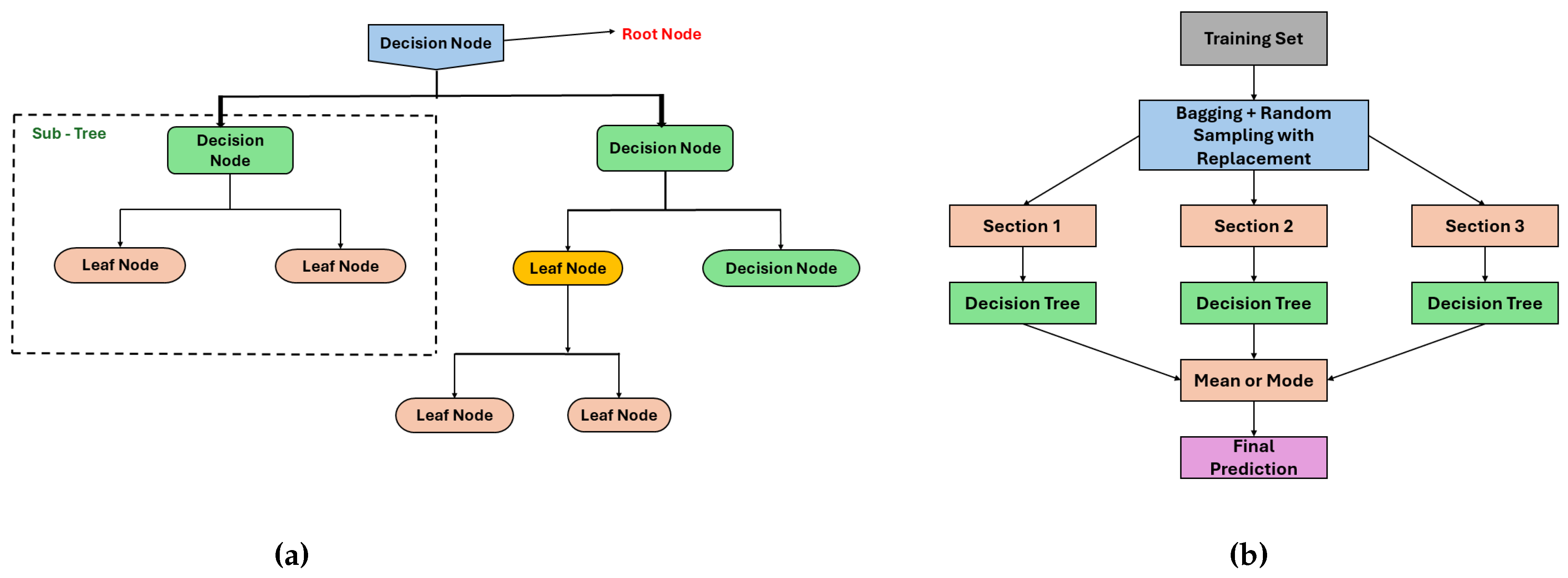
Decision tree (DT) regression is one of the effective and comprehensible machine learning methods to forecast continuous outcomes. DT regressor divides the feature space into multiple sub-regions and assigns a constant value to each region for modeling, in contrast to classic regression techniques that fit a single global model to represent the data [53]. The multiple sub-regions are formed through recursive partitioning based on the feature value. Furthermore, optimal splits are determined by minimizing error metrics such as mean square error (MSE), root mean square error (RSME), etc. Each internal node represents a decision based on a feature, each branch denotes the decision’s outcome, and each leaf node corresponds to a predicted value, collectively structured like a tree.
A key benefit of decision trees over other modeling approaches is their ability to generate models that can be expressed as interpretable rules or logical statements. The interpretability of trees that create axis-parallel decision boundaries offers a significant advantage [54]. Additionally, classification using decision trees does not require complex computation, and the method is applicable to both continuous and categorical variables. Moreover, decision tree models offer transparent insights into the relative importance of key factors in prediction or classification tasks.
In this study, hyperparameter maximum depth limits the number of splits to avoid overfitting, as deeper trees tend to capture intricate patterns; however, may overfit on small datasets. The criterion (for example, gini impurity for classification or squared error for regression) determines the splitting points for impurity reduction and optimization. Additionally, the minimum sample split parameter controls the minimum number of samples required to split a node, preventing unnecessary splits. Furthermore, the minimum sample leaf parameter ensures that each leaf node has at least a minimum number of samples, aiding in generalization by mitigating highly specific decision rules.
2.3.2. Random Forest Regressor (RF)
Random forest is a predictor that is made up of an assortment of M-randomized regression trees, where a random subset of training data are used to construct each tree. The term “random forests” can be interpreted in different ways. Some scholars describe it as a generic expression for aggregating random decision trees regardless of how trees are obtained, while others refers to Breiman’s (2001) original algorithm[55]. Random forest is an ensemble learning technique that combines multiple decision trees to increase accuracy and reduce overfitting. Similarly, trees are generated independently, allowing the process to be parallelized for better computation. Unlike a single decision tree that is prone to the overfitting problem, the RF model leverages bagging (Bootstrap Aggregation) and random feature selection to reduce variance while maintaining interpretability. Mathematically, RF follows the bagging approach, where each individual tree is trained on a bootstrapped dataset drawn from the original dataset.
where represents feature vectors and represents the target values. Each tree is trained on a subset of the original data, and each subset is drawn randomly from D with replacement.
For regression, the final prediction is obtained by averaging the predictions from all B trees:
In this paper, the hyperparameter "number of trees" is controlled with the estimator parameter. The increasing number of trees enhances the predictive performance; however, it results in higher computational expense. Minimum samples split and minimum samples per leaf operate as pruning parameters for decision trees, controlling the growth of trees and pruning. Furthermore, max feature controls the number of features considered for splitting in each step to reduce overfitting through the application of diversity across trees. Bootstrap sampling controls training each tree on a random subsample of data that reduces the variance and promotes generalization in the model.
Figure 4.
Graphical Representation of (a) Decision Tree (b) Random Forest.
2.3.3. K-Nearest Neighbor Regressor (KNN)
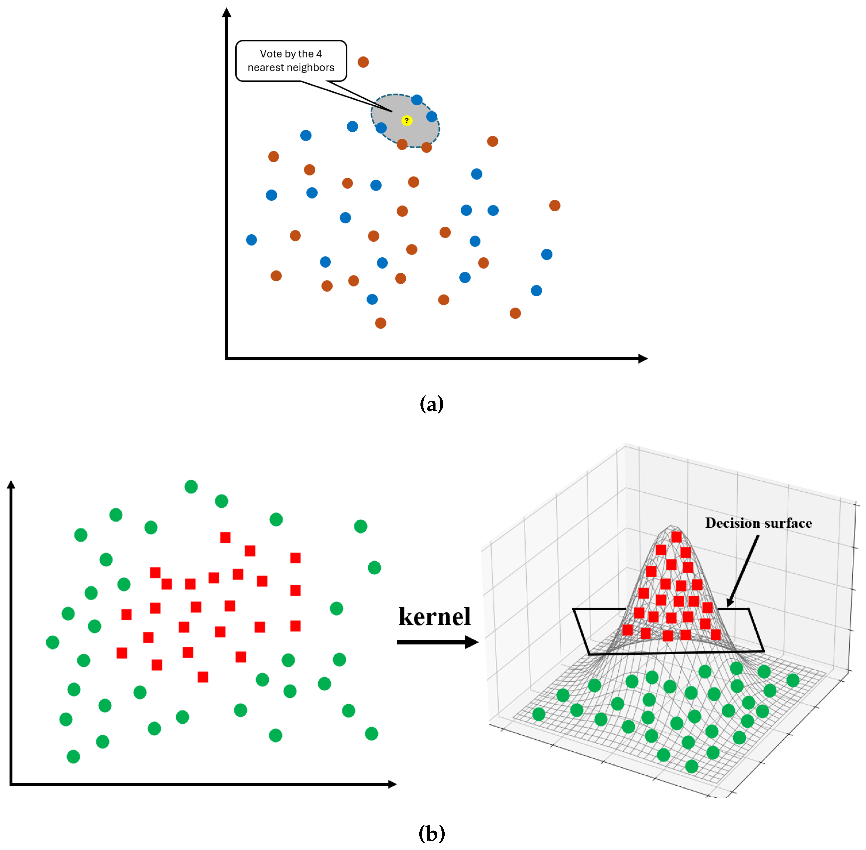
K-Nearest Neighbors (KNN) is a basic machine learning algorithm that can be implemented for classification and regression tasks. It is a supervised learning method that operates on the idea that data points with similar features are located near proximity of each other within a feature space. In KNN regression, the prediction for a new data point is obtained by averaging the target values of its closest neighbors, which are identified using a distance metric such as the Euclidean or Manhattan distance.
The KNN algorithm predicts outcomes through a simple process, as illustrated in Figure 5a. Initially, the number of neighbors ’k’ is considered, followed by a distance metric, typically Euclidean distance, to identify the k closest points in the training dataset. Once the nearest neighbors are identified, their output values are averaged (or weighted) to generate the prediction. The expected value can be expressed mathematically as:
where represents the actual output values of the k-nearest neighbors.
Figure 5.
Graphical Representation of (a) KNN (b) SVM.
In this paper, the hyperparameter Neighbor(K) considers the K number of nearest points for the prediction to balance between the bias and variance. When K is small, the model becomes sensitive to noise, whereas larger K results in a smoother decision boundary. Similarly, the hyperparameter p indicates the distance method determined to calculate the distance between points. Furthermore, the weights parameter determines the contribution of the selected neighbor to calculate the output. For instance, in weighted schemes, closer neighbors have more influence on the decision, whereas in uniform schemes, every neighbor has equal weight.
2.3.4. Support Vector Regressor (SVR)
The Support Vector Regressor (SVR) is a machine learning algorithm that is derived based on the Support Vector Machines (SVMs) principles for regression analysis. A standard classification SVM locates a hyperplane to separate different classes with maximum margins [56]. However, SVR computes a specific function that stays close to all data points, as illustrated in Figure 5b. The algorithm maintains a small margin of error epsilon () making the SVR method effective for precise numerical predictions instead of category assignments. The equation provided to minimize the cost function in SVR is:
where:
- -
- controls the model complexity.
- -
- C is a hyperparameter that determines the trade-off between margin size and prediction accuracy.
- -
- -
- -
- are the Slack variables which penalize the error if the prediction is outside the margin.
In this paper, the parameter C controls the trade-off between maximizing the margin and minimizing error. Higher values of C result in a high penalty for misclassifications, making tighter decision boundaries. Epsilon demonstrates relevance in regression-based SVM to define the error tolerance in regression. Similarly, a kernel function (linear, polynomial, radial basis function (RBF), etc.) transforms the input into a higher-dimensional space, making it easier to identify patterns in the data. The gamma parameter controls the influence of individual training points on the decision boundary, such that smaller values result in wider decision boundaries and higher values provide priority to local pattern priority. Thus, hyperparameter tuning is essential for better predictive accuracy as well as model adaptability.
2.4. Errors Computation
Many studies employ the mean square error (MSE) and its rooted variant root mean square error (RMSE), or the mean absolute error (MAE) and its percentage variant (MAPE) as error-based metrics to evaluate the model performance. Although widely utilized due to their simplicity and interpretability, these metrics share a common drawback: unbounded values ranging between zero and positive infinity. Furthermore, a single value provides limited insight into the performance of the regression models with respect to the statistical distribution of the ground truth elements [57]. This paper utilize two primary metrics, RMSE and error (coefficient of determination) for evaluation of model performance. RMSE quantifies the square root of the squared average differences between observed values with predicted values, resulting in a comprehensive measure of prediction accuracy. A lower RMSE reflects lower deviations between actual and predicted values and indicates better model performance. Mathematically, it is given by:
On the other hand, the coefficient of determination ( error) quantifies the extent to which the independent variables explain the variance in the dependent variable. It is computed as:
The value of closer to 1 indicates an excellent model fit, whereas a lower reflects weak predictive capabilities. Unlike RMSE, which measures predictive error in absolute terms, offers a relative assessment by comparing model performance against a baseline - the mean of the target variable. RMSE and serve different purposes in regression analysis: while RMSE measures the accuracy of predictions in absolute terms, explains how variance in target variable is captured by the model. Collectively, these metrics enable in capturing both the magnitude of prediction errors and the overall goodness-of-fit.
2.5. Hyper-parameter tuning
Hyperparameter tuning has a direct influence on models predictive capabilities and is an important step in optimizing model governing parameters. However, determination of the best hyperparameters can be computationally intensive, particularly when determination of objective functions are costly or when the model involves a large number of parameters required to be tuned [58]. Several effective techniques are available for tuning hyperparameters in ML methods, such as Grid Search (GS), Random Search (RS), Bayesian optimization (BO), etc.
In this study, GS optimization method was utilized for hyperparameter tuning due to the lower number of parameters involved with the employed ML models. It is often described as a brute-force or exhaustive search technique [59]. While GS is known for its high accuracy, the computational time required for it is excessive. Grid search (GS) exhaustively searches a manually specified subset of the hyperparameter space of the target algorithm. Unlike RS, which may miss critical combinations due to random sampling from the hyperparameter space, GS evaluates all possible combinations within the predefined grid, offering a more reliable optimization approach. Furthermore, for smaller dataset and fewer associated hyperparameters, BO, with its complexity in setting up surrogate models and acquisition functions, makes it less efficient in this study in comparison to GS.
3. Result and Discussion
The compressive strength of GGP incorporated concrete was analyzed using six individual ML algorithms. The measured compressive strength versus the predicted compressive strength is plotted for each ML algorithm. Figure 6 illustrates the results of the training dataset and the testing dataset for LR, ENR, KNN, DT, RF, and SVM. The RSMEs are 6.95 MPa, 8.20 MPa, 6.56 MPa, 3.88 MPa, 5.70 MPa, and 8.01 MPa for LR, ENR, KNN, DT, RF, and SVM, respectively, for the testing dataset. Similarly, for the test dataset, the values for LR, ENR, KNN, DT, RF, and SVM are 0.80, 0.73, 0.82, 0.94, 0.86, 0.74, respectively. It can be observed that the DT model has predicted the best among the six ML algorithms with of 1.0 for the training dataset and of 0.94 for the testing dataset. However, this perfect value in the training dataset is due to the overfitting problems usually encountered by the DT model. When hyperparameters are not tuned, the DT model generates higher depth trees and tends to memorize the dataset, and ultimately yields reduced performance on unseen testing dataset. For RF, before hyperparameter tuning, the algorithm evaluated of 0.88 for training and 0.82 for the testing dataset, with RSME of 5.56 MPa for training and 6.55 MPa for the testing dataset. Although RF demonstrated relatively better performance compared to other ML models, the little variation in error metrics between the testing and training dataset suggests potential overfitting. Furthermore, the values for LR and ENR before hyperparameter tuning for the testing dataset are below 0.8, which is generally not considered a good fit. Furthermore, KNN and SVR demonstrate moderate generalization capabilities before tuning. RSME values of 6.69 MPa for training and 6.56 MPa for testing by KNN indicate suboptimal performance. Additionally, a high discrepancy between training (RMSE = 5.85 MPa) and testing (RMSE = 8.01 MPa) suggests underfitting for the SVM model. Similarly, LR and ENR demonstrate stable, however, moderate performance with similar RSME values. LR achieved RMSE values of 5.56 MPa and 6.95 MPa for training and testing datasets, respectively, while ENR obtained RMSE values of 8.27 MPa and 8.20 MPa. This suggests lower overfitting problems; however, the prediction accuracy is lower than other models.
The predictive capability of five models: ENR, KNN, DT, RF, and SVM, after respective model hyperparameter tuning are depicted in Figure 7. All machine learning models demonstrate values greater than 0.8 for the test dataset, which is generally considered a good fit. ENR shows a significant increase in its from 0.73 to 0.81 with the reduction in RSME from 8.20 to 6.85 MPa for the test dataset. Similarly, the KNN algorithm also improves the performance with an increase of value from 0.82 to 0.87. Furthermore, the DT model, which initially exhibited a perfect fit on the training data ( = 1 and RSME = 0.0 MPa), demonstrates better generalization with balanced training and testing values of 0.98 and 0.91, respectively. RF model, after hyperparameter tuning, shows improvement in both testing and training performance. The RSME drops from 6.55 MPa to 4.56 MPa and increases from 0.82 to 0.91 for the test dataset, reflecting better predictive accuracy after hyperparameter tuning. SVR benefits greatly from hyperparameter tuning and demonstrates the highest predictive capabilities among the models with value of 0.95 and RMSE of 3.40 MPa for the test dataset. For a small dataset with high dimensionality, SVR outperforms other algorithms such as KNN and DT due to its robustness against the curse of dimensionality. Similarly, for a non-linear dataset, the kernel trick in SVR enables the algorithm to effectively model the complex patterns in higher-dimensional spaces. Through hyperparameters such as the regularization parameter C and loss parameter , SVR can fine-tune the balance between fit and generalization, making it less susceptible to overfitting or underfitting problems. The performance of the six ML models employed in this study before and after hyperparameter tuning is shown in Table 2. Furthermore, finalized hyperparameters associated with each model are summarized in Table 3. Overall, hyperparameter tuning enhances the model performance of all models, reduces the underfitting and overfitting problems, and improves the model predictability for testing and training dataset.
4. Conclusions
It is essential to accurately estimate the compressive strength of concrete to optimize the mix design, reducing the curing duration and the overall cost of the project. In this study, application of different ML algorithms: LN, ENR, KNN, DT, RF, and SVM are employed leveraging 12 influencing input parameters from 188 reliable mixes to predict the compressive strength of concrete. The results indicate favorable evidence of using artificial intelligence approaches to predict compressive strength of concrete incorporated with GGP as a partial cement replacement. The following conclusions are drawn after careful evaluation of each model’s performance:
- LR and ENR exhibits the stable however moderate performance with similar and RSME values before hyperparameter tuning. However, ENR shows a significant increase in value from 0.73 to 0.81 with drop in RSME value from 8.20 to 6.85 MPa for the test dataset after hyperparameter tuning.
- KNN model shows good prediction with the same value of 0.82 for training and testing before hyperparameter tuning. Furthermore, with hyperparameter tuning, the value increased to 0.87 and RMSE decreased to 5.62 MPa for the test dataset.
- The DT tree demonstrates the highest accuracy ( = 1.0 for training, = 0.94 for testing) before hyperparameter tuning due to creation of deep trees. A reduction on overfitting and better generalization with training and testing datasets is observed with hyperparameter tuning.
- The RF model exhibits moderate performance with of 0.82 and RSME of 6.55 MPa for the test dataset. However, after hyperparameter tuning, RSME reduced to 4.56 MPa from 6.55 MPa and improved to 0.91 from 0.82 for the test dataset. This concludes, RF model benefits from hyperparameter tuning, leading to improved generalization.
- SVR demonstrates lower accuracy with of 0.74 and RSME of 8.01 MPa for the test dataset before hyperparameter tuning. However, a significant increase in to 0.95 and a reduction in RSME to 3.40 MPa show superior predictive capability of SVM after hyperparameter tuning.
In conclusion, the ML models demonstrate a reliable predictive accuracy on estimating the CS of GGP incorporated concrete. The practical implications of these findings can be a significant help in promoting sustainability within the construction industry. These models would enable the optimization of the GGP content in the concrete mix design, contributing directly to lowering cement demand and associated emission, which are a major contributor to global warming. Furthermore, the use of waste glass as a SCM in concrete diverts glass from landfill sites, promoting a circular economy. With the data considered, SVR outperforms other ML algorithms in the prediction of the compressive strength of concrete incorporating GGP. SVM, with its high accuracy, has the potential to be used as a prediction tool to optimize the mix design, overall cost of future projects, and support sustainable construction practices.
Author Contributions
Writing original draft, Sushant Poudel and Bibek Gautam; conceptualization, Sushant Poudel, Diwakar KC, and Yong Je Kim; methodology, Sushant Poudel, Bibek Gautam, Diwakar KC and Yong Je Kim ; formal analysis, Sushant Poudel, Bibek Gautam, Utkarsha Bhetuwal, Pravin Kharel, Sudip Khatiwada, Subash Dhital; investigation, Sushant Poudel, Bibek Gautam, Utkarsha Bhetuwal, Pravin Kharel, Sudip Khatiwada, Subash Dhital; resources, Sudip Khatiwada, Diwakar KC, nad Yong Je Kim; review and editing, Sushant Poudel, Bibek Gautam, Utkarsha Bhetuwal, Sudip Khatiwada, Subash Dhital, and Diwakar Kc; data collection, Sushant Poudel, Pravin Kharel, Subash Dhital; grammatical improvement, Sudip Khatiwada. Diwakar KC, and Yong Je Kim; formatting, Sudip Khatiwada; revising, Sushant Poudel, Bibek Gautam, , Utkarsha Bhetuwal, Pravin Kharel and Subash Dhital. All authors have read and agreed to the published version of the manuscript.
Funding
This research received no external funding.
Data Availability Statement
All data are available in the manuscript.
Acknowledgments
We would like to thank Professor Venkatesh Uddameri for his guidance in applying machine learning techniques to civil engineering, which laid the foundation for this work.
Conflicts of Interest
Author Diwakar KC was employed by the company Universal Engineering Sciences. The remaining authors declare that the research was conducted in the absence of any commercial or financial relationships that could be construed as a potential conflict of interest.
References
- Feng, D.C.; Liu, Z.T.; Wang, X.D.; Chen, Y.; Chang, J.Q.; Wei, D.F.; Jiang, Z.M. Machine learning-based compressive strength prediction for concrete: An adaptive boosting approach. Construction and Building Materials 2020, 230, 117000. [Google Scholar] [CrossRef]
- Yehia, S.A.; Shahin, R.I.; Fayed, S. Compressive behavior of eco-friendly concrete containing glass waste and recycled concrete aggregate using experimental investigation and machine learning techniques. Construction and Building Materials 2024, 436, 137002. [Google Scholar] [CrossRef]
- Chopra, P.; Sharma, R.K.; Kumar, M.; Chopra, T. Comparison of machine learning techniques for the prediction of compressive strength of concrete. Advances in Civil Engineering 2018, 2018, 5481705. [Google Scholar] [CrossRef]
- Elmikass, A.G.; Makhlouf, M.H.; Mostafa, T.S.; Hamdy, G.A. Experimental Study of the Effect of Partial Replacement of Cement with Glass Powder on Concrete Properties. Key Engineering Materials 2022, 921, 231–238. [Google Scholar] [CrossRef]
- Abdelli, H.E.; Mokrani, L.; Kennouche, S.; de Aguiar, J.B. Utilization of waste glass in the improvement of concrete performance: A mini review. Waste Management & Research 2020, 38, 1204–1213. [Google Scholar]
- Muhedin, D.A.; Ibrahim, R.K. Effect of waste glass powder as partial replacement of cement & sand in concrete. Case Studies in Construction Materials 2023, 19, e02512. [Google Scholar]
- Paul, S.C.; Šavija, B.; Babafemi, A.J. A comprehensive review on mechanical and durability properties of cement-based materials containing waste recycled glass. Journal of Cleaner Production 2018, 198, 891–906. [Google Scholar] [CrossRef]
- Althoey, F.; Ansari, W.S.; Sufian, M.; Deifalla, A.F. Advancements in low-carbon concrete as a construction material for the sustainable built environment. Developments in the built environment 2023, 16, 100284. [Google Scholar] [CrossRef]
- Chousidis, N.; Rakanta, E.; Ioannou, I.; Batis, G. Mechanical properties and durability performance of reinforced concrete containing fly ash. Construction and Building Materials 2015, 101, 810–817. [Google Scholar] [CrossRef]
- Ramakrishnan, K.; Pugazhmani, G.; Sripragadeesh, R.; Muthu, D.; Venkatasubramanian, C. Experimental study on the mechanical and durability properties of concrete with waste glass powder and ground granulated blast furnace slag as supplementary cementitious materials. Construction and Building Materials 2017, 156, 739–749. [Google Scholar] [CrossRef]
- Teng, S.; Lim, T.Y.D.; Divsholi, B.S. Durability and mechanical properties of high strength concrete incorporating ultra fine ground granulated blast-furnace slag. Construction and Building Materials 2013, 40, 875–881. [Google Scholar] [CrossRef]
- Alharthai, M.; Onyelowe, K.C.; Ali, T.; Qureshi, M.Z.; Rezzoug, A.; Deifalla, A.; Alharthi, K. Enhancing concrete strength and durability through incorporation of rice husk ash and high recycled aggregate. Case Studies in Construction Materials 2025, 22, e04152. [Google Scholar] [CrossRef]
- Banerji, S.; Poudel, S.; Thomas, R.J. Performance of Concrete with Ground Glass Pozzolan as Partial Cement Replacement.
- Tural, H.; Ozarisoy, B.; Derogar, S.; Ince, C. Investigating the governing factors influencing the pozzolanic activity through a database approach for the development of sustainable cementitious materials. Construction and Building Materials 2024, 411, 134253. [Google Scholar] [CrossRef]
- Olaiya, B.C.; Lawan, M.M.; Olonade, K.A.; Segun, O.O. An overview of the use and process for enhancing the pozzolanic performance of industrial and agricultural wastes in concrete. Discover Applied Sciences 2025, 7, 164. [Google Scholar] [CrossRef]
- Poudel, S.; Bhetuwal, U.; Kharel, P.; Khatiwada, S.; KC, D.; Dhital, S.; Lamichhane, B.; Yadav, S.K.; Suman, S. Waste Glass as Partial Cement Replacement in Sustainable Concrete: Mechanical and Fresh Properties Review. Buildings 2025, 15, 857. [Google Scholar] [CrossRef]
- Miao, X.; Chen, B.; Zhao, Y. Prediction of compressive strength of glass powder concrete based on artificial intelligence. Journal of Building Engineering 2024, 91, 109377. [Google Scholar] [CrossRef]
- Song, H.; Ahmad, A.; Farooq, F.; Ostrowski, K.A.; Maślak, M.; Czarnecki, S.; Aslam, F. Predicting the compressive strength of concrete with fly ash admixture using machine learning algorithms. Construction and Building Materials 2021, 308, 125021. [Google Scholar] [CrossRef]
- Bhandari, I.; Kumar, R.; Sofi, A.; Nighot, N.S. A systematic study on sustainable low carbon cement – Superplasticizer interaction: Fresh, mechanical, microstructural and durability characteristics. Heliyon 2023, 9, e19176. [Google Scholar] [CrossRef]
- Linderoth, O.; Wadsö, L.; Jansen, D. Long-term cement hydration studies with isothermal calorimetry. Cement and Concrete Research 2021, 141, 106344. [Google Scholar] [CrossRef]
- Jin, L.; Duan, J.; Jin, Y.; Xue, P.; Zhou, P. Prediction of HPC compressive strength based on machine learning. Scientific Reports 2024, 14, 16776. [Google Scholar] [CrossRef]
- Wilson, A.; Anwar, M.R. The Future of Adaptive Machine Learning Algorithms in High-Dimensional Data Processing. International Transactions on Artificial Intelligence 2024, 3, 97–107. [Google Scholar] [CrossRef]
- Sarker, I.H. Machine learning: Algorithms, real-world applications and research directions. SN computer science 2021, 2, 160. [Google Scholar] [CrossRef] [PubMed]
- Hajkowicz, S.; Sanderson, C.; Karimi, S.; Bratanova, A.; Naughtin, C. Artificial intelligence adoption in the physical sciences, natural sciences, life sciences, social sciences and the arts and humanities: A bibliometric analysis of research publications from 1960-2021. Technology in Society 2023, 74, 102260. [Google Scholar] [CrossRef]
- Niu, X.; Wang, L.; Yang, X. A comparison study of credit card fraud detection: Supervised versus unsupervised. arXiv preprint arXiv:1904.10604 2019. [CrossRef]
- Hamed, A.K.; Elshaarawy, M.K.; Alsaadawi, M.M. Stacked-based machine learning to predict the uniaxial compressive strength of concrete materials. Computers & Structures 2025, 308, 107644. [Google Scholar]
- Bentegri, H.; Rabehi, M.; Kherfane, S.; Nahool, T.A.; Rabehi, A.; Guermoui, M.; Alhussan, A.A.; Khafaga, D.S.; Eid, M.M.; El-Kenawy, E.S.M. Assessment of compressive strength of eco-concrete reinforced using machine learning tools. Scientific Reports 2025, 15, 5017. [Google Scholar] [CrossRef]
- Sathiparan, N. Predicting compressive strength in cement mortar: The impact of fly ash composition through machine learning. Sustainable Chemistry and Pharmacy 2025, 43, 101915. [Google Scholar] [CrossRef]
- Sinkhonde, D.; Bezabih, T.; Mirindi, D.; Mashava, D.; Mirindi, F. Ensemble machine learning algorithms for efficient prediction of compressive strength of concrete containing tyre rubber and brick powder. Cleaner Waste Systems 2025, 100236. [Google Scholar] [CrossRef]
- Abdellatief, M.; Murali, G.; Dixit, S. Leveraging machine learning to evaluate the effect of raw materials on the compressive strength of ultra-high-performance concrete. Results in Engineering 2025, 25, 104542. [Google Scholar] [CrossRef]
- Dong, Y.; Tang, J.; Xu, X.; Li, W.; Feng, X.; Lu, C.; Hu, Z.; Liu, J. A new method to evaluate features importance in machine-learning based prediction of concrete compressive strength. Journal of Building Engineering 2025, 111874. [Google Scholar] [CrossRef]
- Bypour, M.; Yekrangnia, M.; Kioumarsi, M. Machine Learning-Driven Optimization for Predicting Compressive Strength in Fly Ash Geopolymer Concrete. Cleaner Engineering and Technology 2025, 100899. [Google Scholar] [CrossRef]
- Bashir, A.; Gupta, M.; Ghani, S. Machine intelligence models for predicting compressive strength of concrete incorporating fly ash and blast furnace slag. Modeling Earth Systems and Environment 2025, 11, 129. [Google Scholar] [CrossRef]
- Jamal, A.S.; Ahmed, A.N. Estimating compressive strength of high-performance concrete using different machine learning approaches. Alexandria Engineering Journal 2025, 114, 256–265. [Google Scholar] [CrossRef]
- Khan, A.U.; Asghar, R.; Hassan, N.; Khan, M.; Javed, M.F.; Othman, N.A.; Shomurotova, S. Predictive modeling for compressive strength of blended cement concrete using hybrid machine learning models. Multiscale and Multidisciplinary Modeling, Experiments and Design 2025, 8, 25. [Google Scholar] [CrossRef]
- Nikoopayan Tak, M.S.; Feng, Y.; Mahgoub, M. Advanced Machine Learning Techniques for Predicting Concrete Compressive Strength. Infrastructures 2025, 10, 26. [Google Scholar] [CrossRef]
- Sah, A.K.; Hong, Y.M. Performance comparison of machine learning models for concrete compressive strength prediction. Materials 2024, 17, 2075. [Google Scholar] [CrossRef]
- Khan, K.; Ahmad, W.; Amin, M.N.; Rafiq, M.I.; Arab, A.M.A.; Alabdullah, I.A.; Alabduljabbar, H.; Mohamed, A. Evaluating the effectiveness of waste glass powder for the compressive strength improvement of cement mortar using experimental and machine learning methods. Heliyon 2023, 9. [Google Scholar] [CrossRef]
- Ben Seghier, M.E.A.; Golafshani, E.M.; Jafari-Asl, J.; Arashpour, M. Metaheuristic-based machine learning modeling of the compressive strength of concrete containing waste glass. Structural Concrete 2023, 24, 5417–5440. [Google Scholar] [CrossRef]
- Alkadhim, H.A.; Amin, M.N.; Ahmad, W.; Khan, K.; Nazar, S.; Faraz, M.I.; Imran, M. Evaluating the strength and impact of raw ingredients of cement mortar incorporating waste glass powder using machine learning and SHapley additive ExPlanations (SHAP) methods. Materials 2022, 15, 7344. [Google Scholar] [CrossRef]
- Qasem, O.A.M.A. The Utilization Of Glass Powder As Partial Replacement Material For The Mechanical Properties Of Concrete. PhD thesis, Universitas Islam Indonesia, 2024.
- Shao, Y.; Lefort, T.; Moras, S.; Rodriguez, D. Studies on concrete containing ground waste glass. Cement and concrete research 2000, 30, 91–100. [Google Scholar] [CrossRef]
- Tamanna, N.; Tuladhar, R. Sustainable use of recycled glass powder as cement replacement in concrete. The Open Waste Management Journal 2020, 13, 1–13. [Google Scholar] [CrossRef]
- Kim, S.K.; Kang, S.T.; Kim, J.K.; Jang, I.Y. Effects of particle size and cement replacement of LCD glass powder in concrete. Advances in Materials Science and Engineering 2017, 2017, 3928047. [Google Scholar] [CrossRef]
- Balasubramanian, B.; Krishna, G.G.; Saraswathy, V.; Srinivasan, K. Experimental investigation on concrete partially replaced with waste glass powder and waste E-plastic. Construction and Building Materials 2021, 278, 122400. [Google Scholar] [CrossRef]
- Khan, F.A.; Fahad, M.; Shahzada, K.; Alam, H.; Ali, N. Utilization of waste glass powder as a partial replacement of cement in concrete. Magnesium 2015, 2. [Google Scholar]
- Kamali, M.; Ghahremaninezhad, A. Effect of glass powders on the mechanical and durability properties of cementitious materials. Construction and building materials 2015, 98, 407–416. [Google Scholar] [CrossRef]
- Zidol, A.; Tognonvi, M.T.; Tagnit-Hamou, A. Effect of glass powder on concrete sustainability. New Journal of Glass and Ceramics 2017, 7, 34–47. [Google Scholar] [CrossRef]
- Pedregosa, F.; Varoquaux, G.; Gramfort, A.; Michel, V.; Thirion, B.; Grisel, O.; Blondel, M.; Prettenhofer, P.; Weiss, R.; Dubourg, V.; et al. Scikit-learn: Machine Learning in Python. Journal of Machine Learning Research 2011, 12, 2825–2830. [Google Scholar]
- Van Rossum, G.; Drake Jr, F.L. Python reference manual; Centrum voor Wiskunde en Informatica Amsterdam, 1995.
- Khademi, F.; Behfarnia, K. Evaluation of concrete compressive strength using artificial neural network and multiple linear regression models 2016.
- Kelly, J.W.; Degenhart, A.D.; Siewiorek, D.P.; Smailagic, A.; Wang, W. Sparse linear regression with elastic net regularization for brain-computer interfaces. In Proceedings of the 2012 Annual International Conference of the IEEE Engineering in Medicine and Biology Society. IEEE, 2012, pp. 4275–4278. [CrossRef]
- Czajkowski, M.; Kretowski, M. The role of decision tree representation in regression problems–An evolutionary perspective. Applied soft computing 2016, 48, 458–475. [Google Scholar] [CrossRef]
- Pekel, E. Estimation of soil moisture using decision tree regression. Theoretical and Applied Climatology 2020, 139, 1111–1119. [Google Scholar] [CrossRef]
- Biau, G.; Scornet, E. A random forest guided tour. Test 2016, 25, 197–227. [Google Scholar] [CrossRef]
- Jakkula, V. Tutorial on support vector machine (svm). School of EECS, Washington State University 2006, 37, 3. [Google Scholar]
- Chicco, D.; Warrens, M.J.; Jurman, G. The coefficient of determination R-squared is more informative than SMAPE, MAE, MAPE, MSE and RMSE in regression analysis evaluation. Peerj computer science 2021, 7, e623. [Google Scholar] [CrossRef] [PubMed]
- Hossain, M.R.; Timmer, D. Machine learning model optimization with hyper parameter tuning approach. Glob. J. Comput. Sci. Technol. D Neural Artif. Intell 2021, 21, 31. [Google Scholar]
- Açikkar, M. Fast grid search: A grid search-inspired algorithm for optimizing hyperparameters of support vector regression. Turkish Journal of Electrical Engineering and Computer Sciences 2024, 32, 68–92. [Google Scholar] [CrossRef]
Figure 1.
Pearson correlation matrix for input features
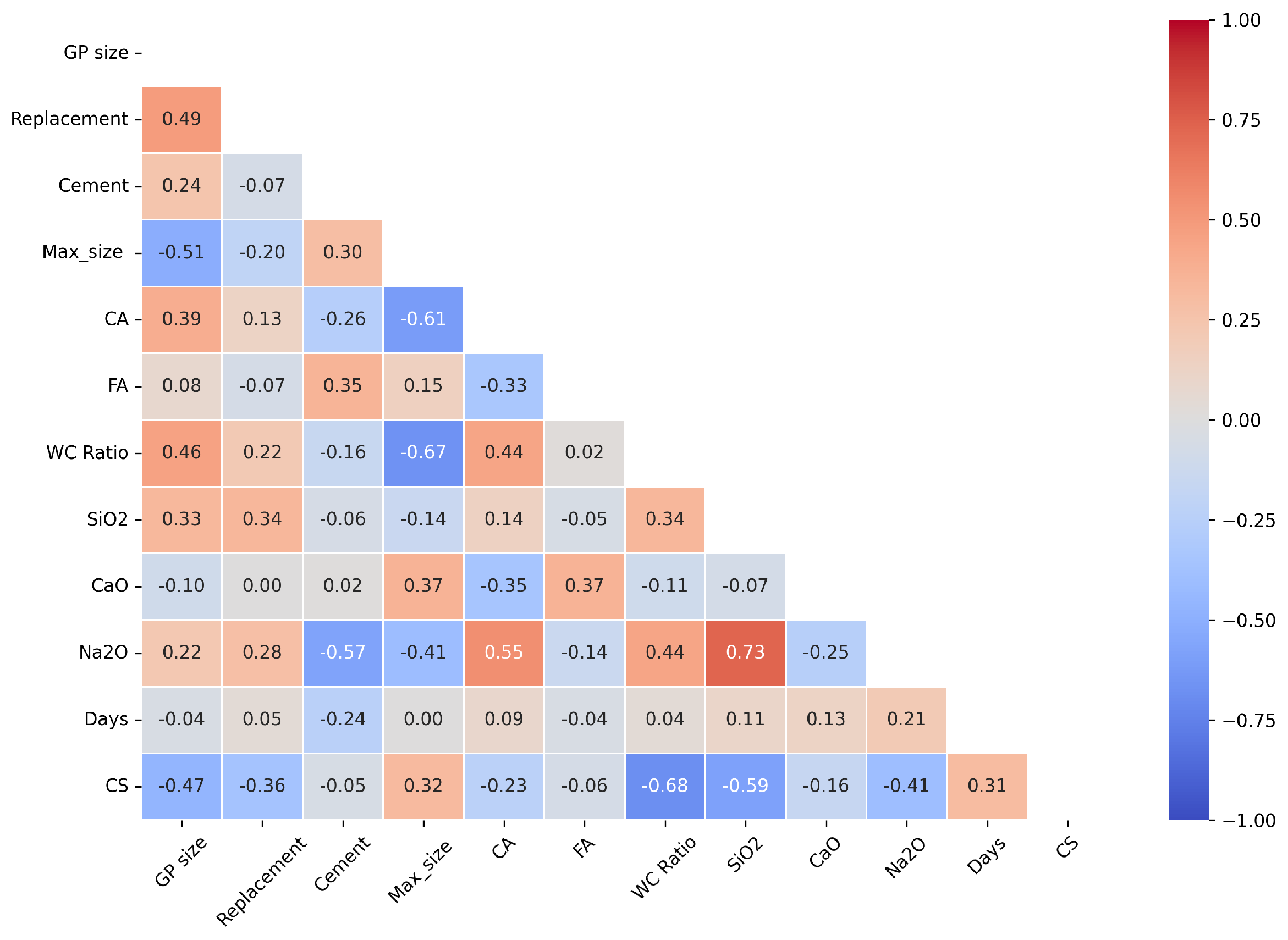
Figure 2.
Marginal plot of compressive strength of concrete with (a) GGP size; (b) GGP replacement Level; (c) cement content; (d) maximum aggregate size; (e) coarse aggregate; (f) fine aggregagte; (g) W/C; (h) ; (i) CaO; (j) O; (k) curing days; (l) compressive strength.
Figure 2.
Marginal plot of compressive strength of concrete with (a) GGP size; (b) GGP replacement Level; (c) cement content; (d) maximum aggregate size; (e) coarse aggregate; (f) fine aggregagte; (g) W/C; (h) ; (i) CaO; (j) O; (k) curing days; (l) compressive strength.
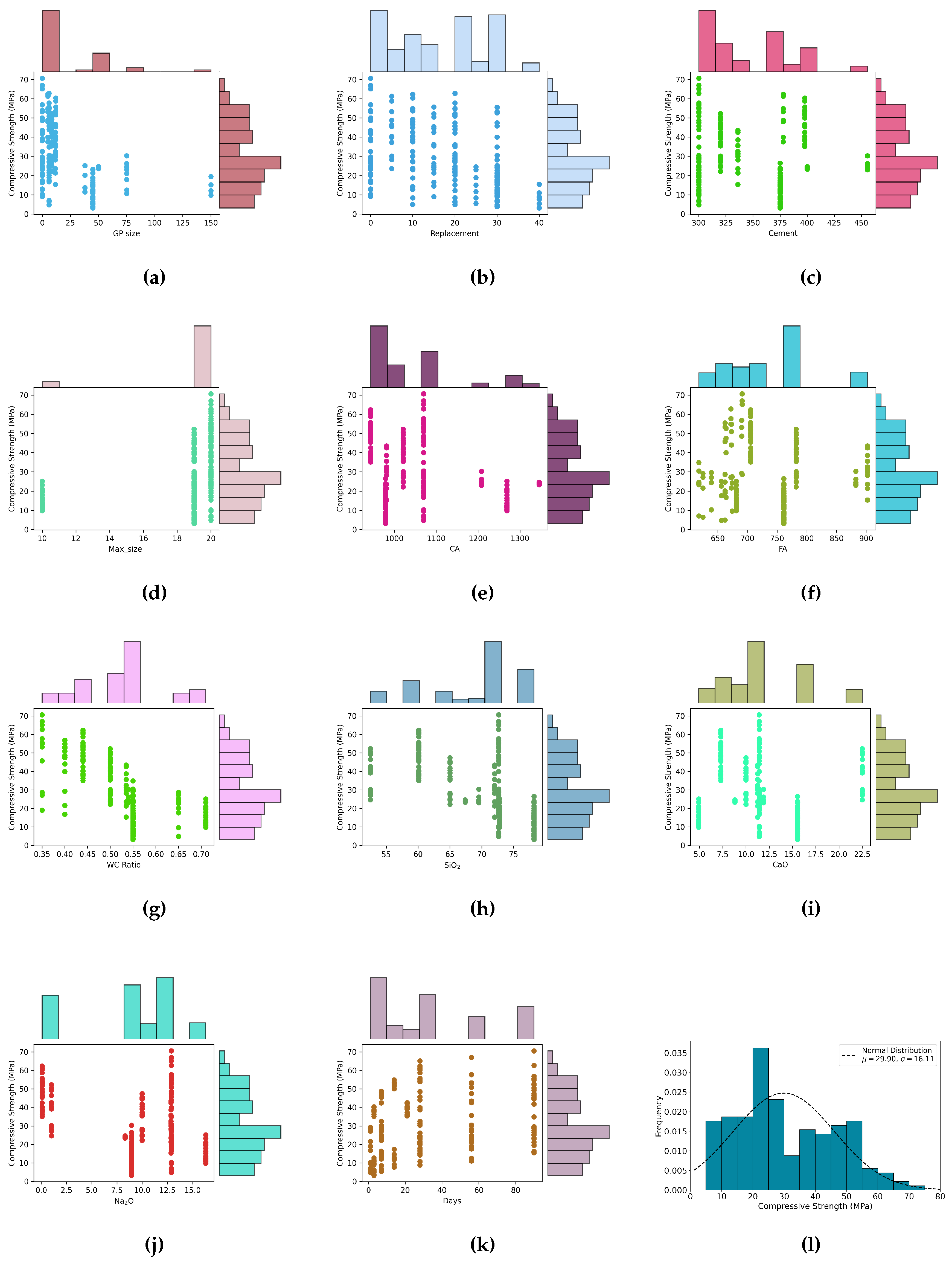
Figure 3.
Flowchart illustrating application of ML.
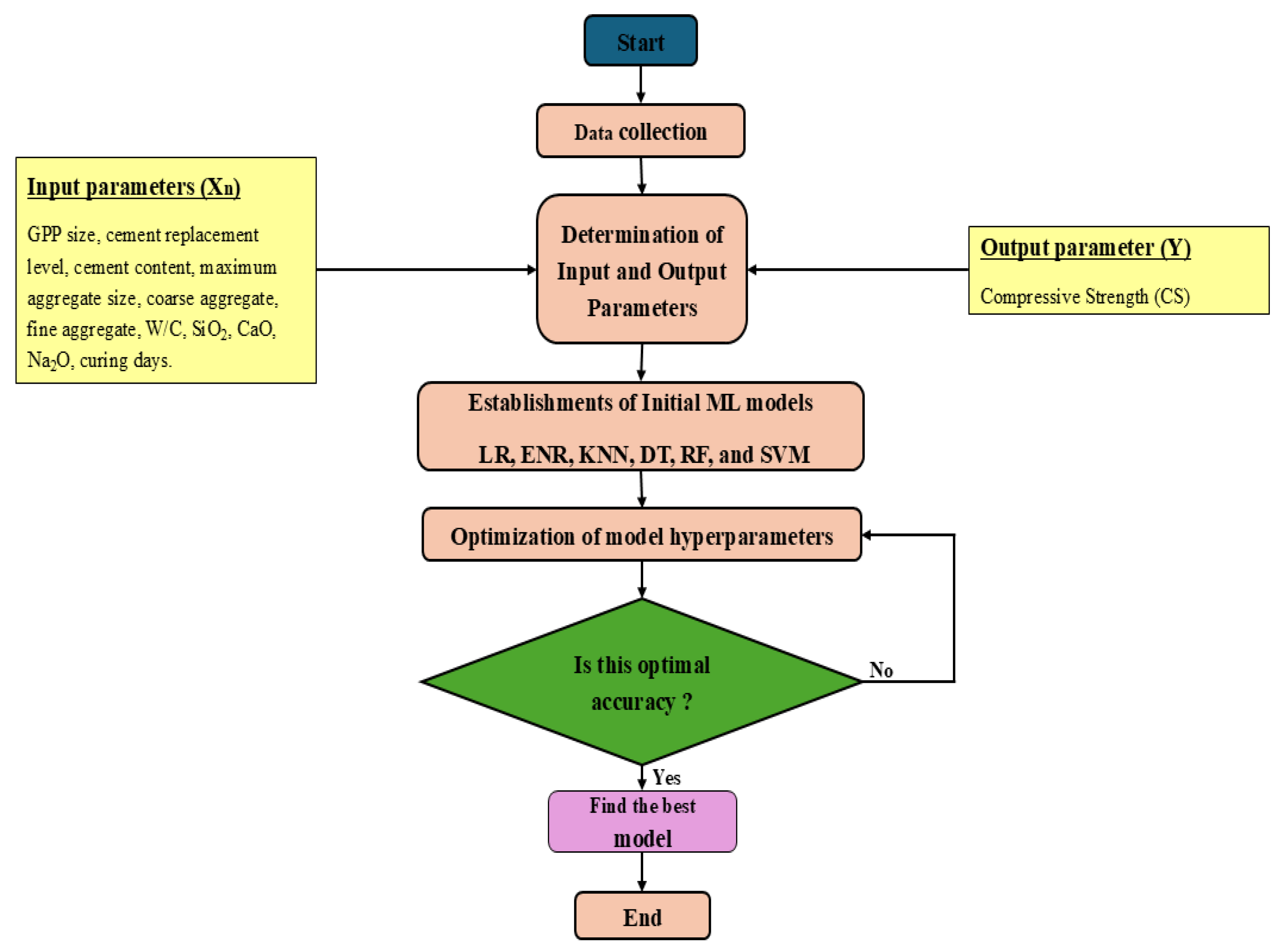
Figure 6.
Comparision between measured and predicted compressive strength of GGP incorporated concrete using different ML algorithms.
Figure 6.
Comparision between measured and predicted compressive strength of GGP incorporated concrete using different ML algorithms.
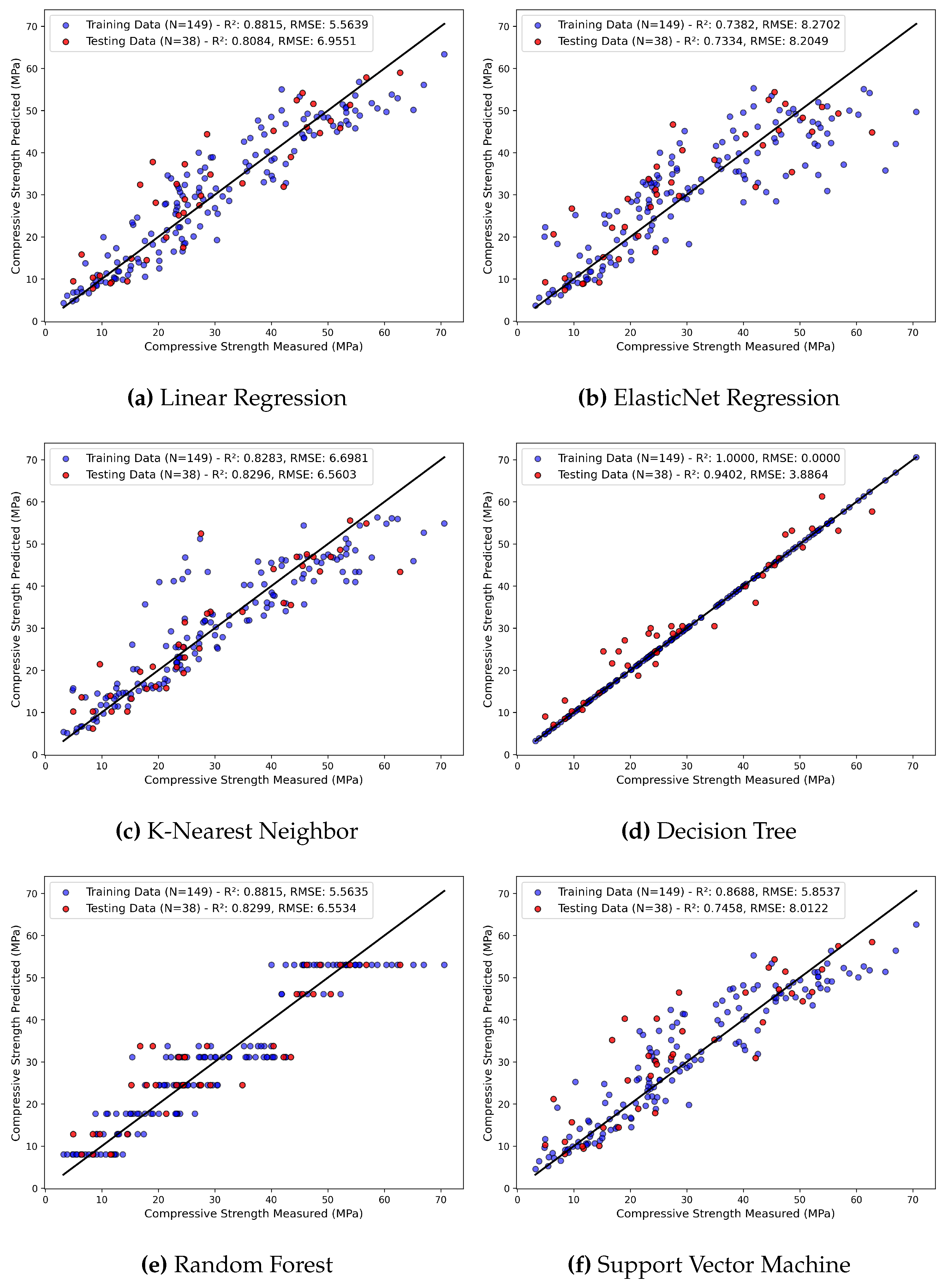
Figure 7.
Comparison between measured and predicted compressive strength of GGP incorporated concrete using different ML algorithms with hyperparameter tuning.
Figure 7.
Comparison between measured and predicted compressive strength of GGP incorporated concrete using different ML algorithms with hyperparameter tuning.
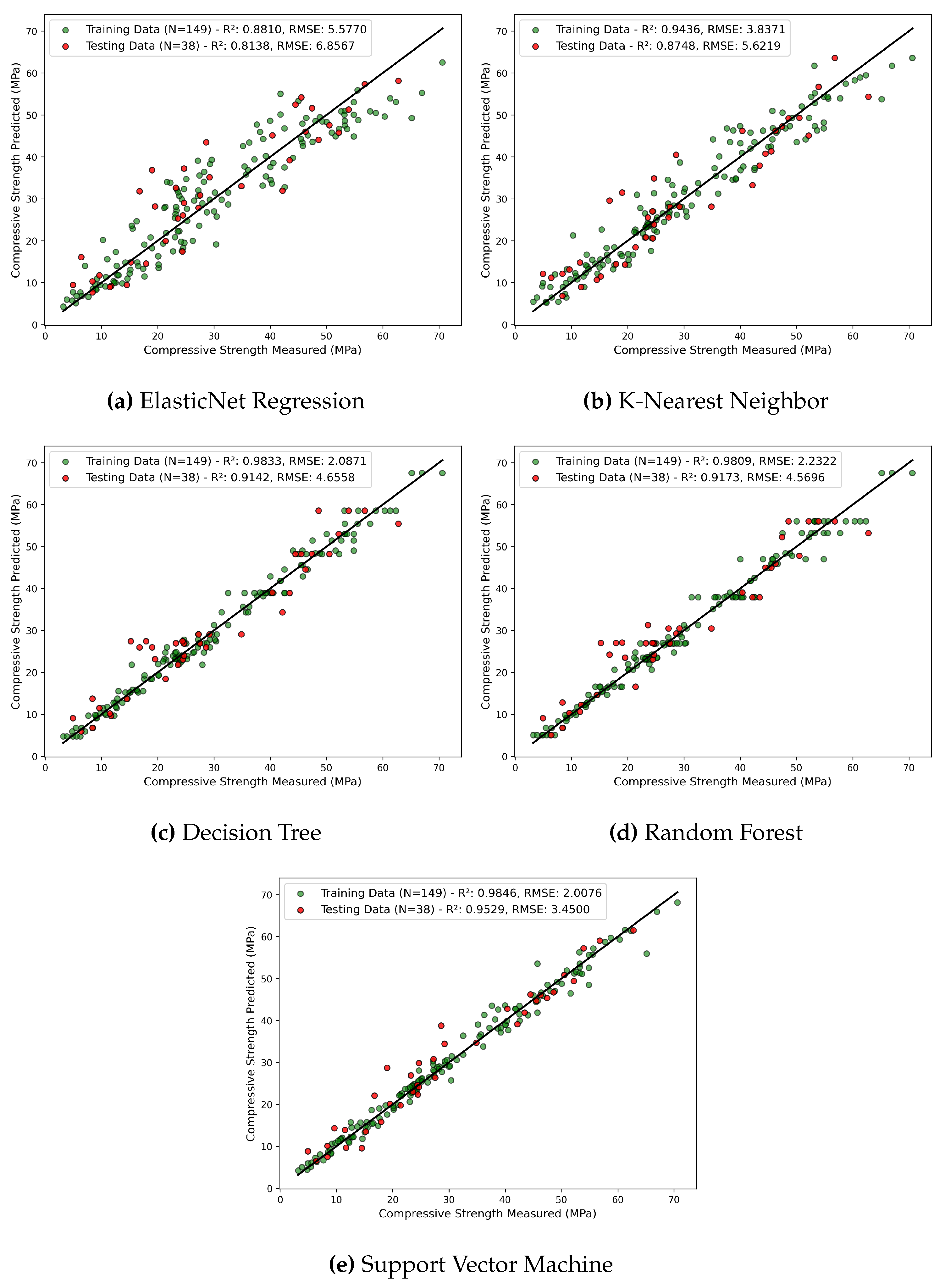

Table 1.
Compressive Strength Test Parameters.
| Parameter | Unit | Minimum | Maximum | Mean | SD | Type |
|---|---|---|---|---|---|---|
| X1: GPP Size | m | 5 | 150 | 27.23 | 29.65 | Input |
| X2: Replacement | - | 5 | 40 | 19.79 | 11.64 | Input |
| X3: W/C | - | 0.35 | 0.71 | 0.5 | 0.09 | Input |
| X4: Cement | 300 | 455.59 | 343.82 | 42.74 | Input | |
| X5: Max size(mm) | mm | 10 | 20 | 18.75 | 2.72 | Input |
| X6: Coarse aggregate | 943.1 | 1346 | 1045.82 | 103.32 | Input | |
| X7: Fine aggregate | 618 | 902 | 732.50 | 72.88 | Input | |
| X8: | % | 52.5 | 78.21 | 69.52 | 7.70 | Input |
| X9: | % | 1.4 | 17.5 | 5.68 | 6.23 | Input |
| X10: CaO | % | 4.9 | 22.5 | 11.87 | 4.48 | Input |
| X11: O | % | 0.08 | 16.3 | 8.93 | 5.16 | Input |
| X12: Curing time | days | 1 | 90 | 33.22 | 30.85 | Input |
| Y: Compressive strength | MPa | 3.19 | 70.6 | 29.90 | 16.11 | Output |
Table 2.
Model performance before and after hyperparameter tuning
| Model | Before Hyperparameter Tuning | After Hyperparameter Tuning | |||||||||
|---|---|---|---|---|---|---|---|---|---|---|---|
| Training Data | Testing Data | Training Data | Testing Data | ||||||||
| RMSE | RMSE | RMSE | RMSE | ||||||||
| Linear Regression | 5.56 | 0.88 | 6.95 | 0.80 | – | – | – | – | |||
| ElasticNet Regression | 8.27 | 0.73 | 8.20 | 0.73 | 5.57 | 0.88 | 6.85 | 0.81 | |||
| K-Nearest Neighbor | 6.69 | 0.82 | 6.56 | 0.82 | 3.83 | 0.94 | 5.62 | 0.87 | |||
| Decision Tree | 0.00 | 1.00 | 3.88 | 0.94 | 2.08 | 0.98 | 4.65 | 0.91 | |||
| Random Forest | 5.56 | 0.88 | 6.55 | 0.82 | 2.23 | 0.98 | 4.56 | 0.91 | |||
| Support Vector Machine | 5.85 | 0.86 | 8.01 | 0.74 | 2.00 | 0.98 | 3.40 | 0.95 | |||
Table 3.
Finalized hyper-parameters.
| ENR | KNN | DT | RF | SVM |
|---|---|---|---|---|
| alpha = 0.01 | Neighbors = 3 | Max depth = 7 | No. of estimators = 79 | C = 100 |
| L1 ratio = 0.987 | p = 2 | criterion = squared error | Minimum samples splits = 2 | Epsilon = 0.1 |
| Weights = uniform | Min samples split= 3 | Minimum samples leaf = 1 | Kernel = rbf | |
| Min samples leaf = 2 | bootstrap = False | Gamma = 0.1 |
Disclaimer/Publisher’s Note: The statements, opinions and data contained in all publications are solely those of the individual author(s) and contributor(s) and not of MDPI and/or the editor(s). MDPI and/or the editor(s) disclaim responsibility for any injury to people or property resulting from any ideas, methods, instructions or products referred to in the content. |
© 2025 by the authors. Licensee MDPI, Basel, Switzerland. This article is an open access article distributed under the terms and conditions of the Creative Commons Attribution (CC BY) license (http://creativecommons.org/licenses/by/4.0/).
Copyright: This open access article is published under a Creative Commons CC BY 4.0 license, which permit the free download, distribution, and reuse, provided that the author and preprint are cited in any reuse.


