Submitted:
20 August 2025
Posted:
21 August 2025
You are already at the latest version
Abstract
Learning systems have played a significant role in classification, Learning sys tems have shaped classification, clustering, regression, and pattern learning problems within the past few decades. Machine learning and deep learning continue to churn out newer models that have transformed the areas of natural language processing, computer vision, speech recognition, recommender sys tems, among others. The evaluation metrics serve as verification systems and are a tool to benchmark the models presented. Depending on the field of use and kind of application, different metrics have been put forth in the literature. They form the common language between researchers. Commercial projects use these metrics to help companies evaluate the value of a model from both an economic and practical point of view. Moreover, in the absence of standards for measurement and evaluation criteria, it becomes almost impossible to compare the results obtained from similar models. This study aims to classify different metrics in learning systems. Therefore, approximately 250 evaluation metrics in text mining, clustering, image mining, and signal analysis have been presented.
Keywords:
evaluation metrics
; text mining metrics
; clustering metrics
; image mining metrics
1. Introduction
Machine Learning and Deep Learning, having become the twin pillars of artificial intelligence, have attracted attention in recent decades owing to their ability to solve complex problems and automate solutions in many fields, including Natural Language Processing [1], Computer Vision [2], Speech Recognition [3], Recommender Systems [4],medicine [5,6] to signal processing [7], video processing [8], natural language processing [9], large language modeling [10], virtual reality [11], time-series analysis [12,13,14], and educational systems [15]. However, with the development and tuning of a machine learning model, it extends beyond the design of algorithms and training of the algorithm itself; not only are these important steps, but the accurate and systematic evaluative assessment of the performance of these models is, in fact, one of the key important steps in the development process. Evaluation metrics assist model builders in measuring quantifiably and qualitatively the strengths and weaknesses of a model [16]. These metrics have become vital to secure the reliability, accuracy, and efficiency of a model’s differential applications in the real world [17]. A model may perform very well in a hypothetical world; however, assuming no accurate metric is at hand, one cannot confidently claim that it will also do well in the real world or when confronted with newer data. Evaluation metrics allow the researchers to investigate the model from various perspectives, such as its generalization property, resistance to overfitting, and behaviour on unbalanced or noisy data. These are important attributes for a developer to consider while making design decisions that affect the improvement, learning procedure, or even choice compared to a more exemplary architecture. Adjusting parameters, providing rewards in training data-choice options to weigh their values, can substantially affect the final performance.
In addition, evaluation metrics serve as a common language among researchers [18]. In commercial projects, these metrics help businesses evaluate the value of a model from an economic and practical perspective. For example, for an image-based medical diagnosis system, the degree of correctness in disease diagnosis or False Positive Rate may directly influence the lives of patients. For text processing applications such as machine translation systems, a metric like BLEU or ROUGE may determine the quality of translation or summarization. Therefore, the choice of the right metric depends not only on the type of problem, but also on the final application of using the model. The evaluation measures used are very diverse depending on the type of problem, i.e., classification, regression, clustering, content creation, etc., and the domain of use, i.e., text, image, audio, etc. There are numerous issues in text processing, including text classification (opinion analysis, sentiment analysis, spam classification), text generation, text summarization, and machine translation. Accuracy, Precision, Recall, and F1-score are prevalent metrics for classification problems. BLEU for translation, ROUGE for summarization, or Perplexity for language models are standard metrics. These metrics help to evaluate the quality of the model’s responses in terms of semantics, structure, and compliance with human natural language. In image-related problems, such as object recognition, segmentation, and image classification, metrics such as Accuracy, Intersection over Union (IoU), Mean Average Precision (mAP), and Top-k Accuracy are very widely used. Likewise, for speech processing, there are metrics such as Word Error Rate (WER), which are used to evaluate speech-to-text systems. For recommender systems, one uses a metric such as Mean Reciprocal Rank (MRR) to measure the quality of the recommendation ranking. Each of these metrics provides various information about the model’s performance, depending on the type of problem and the application objective. One of the main problems with the use of evaluation metrics is the choice of a metric that most accurately reflects the project goal [19]. In an unbalanced data classification problem, accuracy is misleading on its own, since the model can predict the majority class and perform well, but perform badly in the detection of the minority class. In such cases, metrics such as the F1-score or Area Under the ROC Curve (AUC-ROC) provide more accurate information. Specific metrics are also not calibrated to the end-user’s goals. For example, for a machine translation system, a high BLEU score may indicate structure similarity to the reference text, but does not guarantee the semantic quality of the translation. For this reason, human evaluation is sometimes required alongside automated metrics.
This work aims to provide a comprehensive review of learning system evaluation metrics. Machine learning evaluation metrics are not only a mechanism to measure the performance of models, but also a recipe to improve, compare, and select the optimal models. By providing quantitative and qualitative data, these metrics help developers and researchers construct effective, reliable, and feasible models. Since machine learning problems and domains are different, the use of the right metric is dependent upon a deep knowledge of problem, data, and project goals.
2. Text Mining
Text mining is a nascent and growing field that tries to extract meaningful information from unstructured and structured natural texts. Text Mining converts unstructured text into a structured format to identify meaningful patterns and new insights [20]. By using advanced analytical techniques, such as machine learning algorithms and deep learning algorithms, it is possible to discover hidden relationships in unstructured data. Text is one of the most common data types in a database. These data can be divided into three categories [21]:
- Structured Data: These data are standardized as tables of multiple rows and columns. This makes them easier to store and process. Structured data can include entries such as name, address, and phone number.
- Unstructured Data: These data do not have a predefined and specific format. This data can include text from social media, product reviews, or video and audio files.
- Semi-structured Data: As the name suggests, this data combines structured and unstructured data. Examples of semi-structured data include XML, JSON, and HTML files.
Since nearly 80% of the organizational data in the world is unstructured, text mining is considered a very valuable practice in organizations [22]. Text mining tools and techniques allow us to convert unstructured documents into a structured format for high-quality analysis and insight. This, in turn, improves organizational decision-making and leads to better business outcomes [23]. Text mining includes various applications such as marketing applications, Enabling better CRM [24], security applications [25], deception detection [26], medicine and biology [27], literature-based gene identification [28], academic applications, and research stream analysis. It also includes text mining in the natural language processing of users, such as Named-entity recognition [29], Question answering [30], Automatic summarization [31], Natural language generation and understanding [32], Machine translation [33], Foreign language reading and writing [34], Speech recognition, and text proofing [35], and optical character recognition [36]. Different evaluation criteria depending on the user in text mining are defined in the literature. In this section, an attempt has been made to introduce the most critical evaluation criteria in each field.
2.1. Text Data Augmentation
Recent research on data augmentation for natural language processing, including GAN neural networks, has provided various technological advances. Frameworks, tools, and implementation of text-enhanced data pipelines are promoted. However, the lack of evaluation criteria and methods comparison standards, for various reasons including data and criteria, has made the comparison meaningless. Also, there is a lack of standardization of methods, and textual data enhancement research uses unified criteria to compare different enhancement methods. Therefore, researchers seek relevant evaluation criteria for textual data augmentation techniques. Continuing this section, we have tried to categorize the most important criteria for increasing data for natural language processing [37].
2.1.1. Machine Translation Quality
Human evaluation is the best option for evaluating translation quality in intelligent systems and is considered the ground truth. However, since human evaluation is time-consuming and expensive, it is only possible to evaluate some new output of the model by a group of people. For this purpose, a group of evaluation metrics have been introduced that make it possible to evaluate the models to some extent. In the following, we discuss some of the most important metrics [37].
BLEU Score
The BLEU (Bilingual Evaluation Understudy) score is an automated metric for evaluating the quality of text generated by machine translation (MT) systems by comparing it to one or more reference translations [38]. BLEU assesses how closely a machine-generated translation matches professional human translations, focusing on both accuracy and fluency.
Definition 1.
Mathematically, the BLEU score is defined as:
where:
- N is the maximum n-gram length considered (commonly ).
- is the weight assigned to the precision score of n-grams of order n (typically uniform weights, ).
- is the modified precision for n-grams of order n.
- BP is the brevity penalty that penalizes overly short translations.
Modified n-gram Precision () The modified n-gram precision evaluates translation quality across a multi-sentence test corpus. For each source sentence, which may have multiple reference translations, we compute n-gram matches against all its references. The final precision is calculated by aggregating counts across all sentences in the corpus.
where:
- represents the set of all candidate translations in the test corpus
- is computed as:where are the reference translations for the candidate C
- counts each n-gram occurrence in the candidate translation
Brevity Penalty (BP) The brevity penalty penalizes candidate translations that are shorter than the reference translations to prevent overly concise translations that achieve high precision by omitting necessary content. It is calculated as follows:
where:
- c is the total length (in words) of the candidate translations.
- r is the effective reference length, defined as the sum of the lengths of the reference translations closest to each candidate sentence’s length.
Logarithmic Formulation The BLEU score can also be expressed in the logarithmic domain for clarity:
Note: BLEU scores range from 0 to 1, where a higher score indicates greater similarity to the reference translations. In practice, BLEU scores are often multiplied by 100 to represent them as percentages.
2.1.2. Text Generation Quality
Text generation is the task of producing text similar to human-generated texts with the goal of being indistinguishable by humans. This task is formally known in the literature as “natural language generation”.
Text generation can be investigated with Markov processes or deep generative models such as GANs. The continuation of the most important metrics for evaluating the quality of text generation is given.
- Novelty:Novelty and Diversity are distinct. Novelty covers the difference of the produced text from the training set, while Diversity covers the difference of the produced text from other produced texts. A model can be diverse but not novel. These two criteria are listed below [39]:
-
Diversity: BLEU [38] and Self-BLEU [40] are common metrics for quality and diversity evaluation, respectively:Calculate BLEU score for every generated sentence, and define the average BLEU score to be the Self-BLEU of the document.Discriminative BLEU [41]: For tasks with inherently diverse outputs, such as conversational response generation, where there is a wide range of plausible and acceptable responses, BLEU is introduced as an enhanced version of the traditional BLEU score. Unlike standard BLEU, BLEU incorporates human judgments about the quality of reference texts, making it more discriminative. It rewards matches with high-quality references and penalizes matches with low-quality ones, thereby better aligning with human evaluations. This makes BLEU particularly suitable for tasks like conversational response generation, where the space of valid outputs is vast and subjective. The BLEU score for a corpus is computed as:where BP is the brevity penalty, and is the modified n-gram precision for n-grams of order n. The modified n-gram precision is defined as:where:
- −
- i is index over the test set, and j is index over the set of references for the i-th input message.
- −
- is the minimum number of occurrences of n-gram g in the hypothesis and reference .
- −
- is the human-assigned weight for reference .
-
Fluency: This is a subjective and multidimensional concept that can be related to various criteria, such as readability, clarity, and naturalness of the produced text. The context, purpose and audience of the text production task influence fluency. For example, a fluent text for a news article may differ from a fluent text for a children’s story. The text production fluency depends on the desired program. In technical writing, clarity and precision can be essential. The following evaluation criteria can be used to evaluate fluency [42].SLOR:The Syntactic Log Odds Ratio (SLOR) is a metric designed for the evaluation of fluency in natural language generation (NLG) outputs. Its primary purpose is to assess the fluency of generated sentences without relying on reference sentences, which can be particularly useful in scenarios where references are unavailable or impractical to obtain. The SLOR metric is defined mathematically as follows [43]:In this equation, S represents the sentence being evaluated, is the probability assigned to the sentence by a language model (LM), and is the unigram probability of the sentence, calculated as the product of the probabilities of each individual token in the sentence. The normalization by , the length of the sentence, ensures that the metric accounts for variations in sentence length, allowing for a fair comparison between sentences of different sizes. By leveraging the probabilities from a trained language model, SLOR provides a more nuanced evaluation of fluency, making it a valuable tool for researchers and practitioners in the field of natural language processing.Perplexity(PPL),wang2022perplexity: Perplexity (PPL) is one of the most common criteria for evaluating language models. PPL is a metric used to evaluate the fluency and quality of generated text by language models. It is derived from cross-entropy. Mathematically, the cross-entropy H for a sequence of tokens can be expressed as:where is the predicted probability of the i-th token given the previous tokens. PPL is then defined as the exponentiation of the average cross-entropy:where s is the input sentence and m is the number of tokens in the sequence. A lower PPL value indicates better fluency and quality of the text generated by the model.
-
Sentiment Consistency: In the context of text generation, maintaining sentiment consistency is crucial for ensuring that the generated text aligns with the expected emotional tone of the input prompts. In [45], two primary metrics are introduced to evaluate sentiment consistency in generated continuations: SENTSTD and SENTDIFF. These metrics help assess how well the sentiment of the generated text corresponds to the ground truth.
- SENTSTD (Sentiment Standard Deviation),feng2020genaug: This metric measures the average standard deviation of sentiment scores for each batch of generated continuations, concatenated with their respective input prompts. By calculating the standard deviation across all test examples, a lower SENTSTD value indicates greater consistency in sentiment among the generated continuations. This suggests that the generated texts exhibit a more stable emotional tone.
- SENTDIFF (Sentiment Difference),feng2020genaug: This metric evaluates the average difference in sentiment scores between each batch of continuations and their corresponding ground-truth reviews. By averaging these differences across all test examples, a lower SENTDIFF value indicates that the sentiment of the generated continuations aligns more closely with the ground-truth reviews. This metric is essential for assessing the fidelity of the generated text to the expected sentiment.
-
Semantic content preservation,zhang2019bertscore: This evaluation metric is designed to assess the semantic equivalence between generated text and reference text. Unlike traditional metrics that rely on surface form similarity, this metric leverages contextual embeddings to evaluate how well the meaning of the content is preserved in the generated output. The BERTSCORE metric computes the similarity between tokens in the candidate sentence and those in the reference sentence using cosine similarity of their contextual embeddings. The formula for computing the recall, precision, and F1 scores is given as follows:where:
- −
- x is the reference sentence tokenized into k tokens .
- −
- is the candidate sentence tokenized into l tokens .
- −
- and represent the contextual embeddings of tokens and , respectively.
- −
- is the cosine similarity between vectors a and b.
This approach allows for a more nuanced evaluation of text generation, focusing on the preservation of meaning rather than mere lexical overlap, thereby addressing common pitfalls in traditional n-gram based metrics. To enhance this evaluation, Inverse Document Frequency (IDF) weighting is incorporated, which emphasizes the importance of rare and informative tokens. The Recall metric with IDF weighting is defined as follows:where:- −
- is the IDF score of token , where M is the total number of reference sentences, and is the number of sentences containing .
2.1.3. Character n-gram matches
-
Character n-gram F-score (CHRF),popovic2017chrf++: This evaluation metric assesses the quality of machine translation outputs by leveraging character n-grams. CHRF correlates well with human assessments, particularly for morphologically rich languages. It calculates precision and recall based on character n-grams, making it language-independent and robust against tokenization issues. The general formula for the n-gram based F-score is given by:where:
- −
- is the character n-gram precision, calculated as the average precision across all n-grams from to N.
- −
- is the character n-gram recall, representing the average recall across all n-grams from to N.
- −
- is a parameter that assigns times more weight to recall than to precision, with a typical value of 2 being optimal.
The CHRF score is computed by averaging the precision and recall across n-grams of lengths from 1 to N, where N is typically set to 6 for character n-grams. - CHRF+: CHRF+ enhances the original CHRF metric by incorporating word unigrams alongside character n-grams. This integration aims to improve correlation with direct human assessments by capturing both surface-level and semantic information. The precision and recall for CHRF+ ( and ) are calculated as the combined metrics of both character and word n-grams, averaged across all n-gram lengths.
- CHRF++: CHRF++ further refines the CHRF+ metric by optimizing the combination of character and word n-grams, particularly by incorporating word unigrams and bigrams. This variant enhances correlation with direct human assessments by capturing more contextual information from the text. The precision and recall for CHRF++ ( and ) are computed with enhanced weighting strategies for character and word n-grams, allowing for a more nuanced evaluation.
2.1.4. Prediction quality for classification
In the realm of machine learning and statistical analysis, the evaluation of binary classification models is crucial for understanding their performance and reliability. Various metrics have been developed to summarize the outcomes of these models, each offering unique insights into their predictive capabilities. This section focuses on several key metrics that are commonly employed to assess the quality of predictions in binary classification tasks.
The evaluation of a model’s performance typically begins with the construction of a confusion matrix, which categorizes the predictions into four distinct groups: true positives (TP), true negatives (TN), false positives (FP), and false negatives (FN). These categories form the basis for calculating various performance metrics, which help researchers and practitioners gauge how well their models are performing.
Among the most widely used metrics are Accuracy, Precision, and Recall, each of which provides different perspectives on the model’s effectiveness. Accuracy offers a general measure of correctness, while Precision and Recall focus on the model’s performance concerning the positive class. Additionally, the Macro-F1 Score serves as a harmonic mean of Precision and Recall, providing a balanced evaluation, especially in scenarios with imbalanced class distributions.
Other important metrics include Jaccard Similarity, which quantifies the similarity between predicted and actual sets, and the Matthews Correlation Coefficient (MCC), which is particularly valuable for assessing performance on imbalanced datasets. Finally, the Area Under the Precision-Recall Curve (AUPRC), calculated using the trapezoidal rule, summarizes the model’s performance across various thresholds [48].
where: = True Positives, = True Negatives, = False Positives, and = False Negatives.
Precision measures the accuracy of positive predictions.
Recall measures the ability of a model to find all the relevant cases (true positives).
Explanation: The Macro-F1 Score is calculated as the harmonic mean of total precision and total recall. It averages the F1 scores for each class, treating all classes equally regardless of their support (number of true instances).
Explanation: The Jaccard Similarity measures the similarity between two sets A and B. It is defined as the size of the intersection divided by the size of the union of the sets, providing a value between 0 (no overlap) and 1 (complete overlap).
Explanation: The Matthews Correlation Coefficient (MCC) is a measure of the quality of binary classifications. It considers all four categories of the confusion matrix (True Positives, True Negatives, False Positives, False Negatives) and provides a balanced metric that can be used even when classes are of very different sizes.
Explanation: The Area Under the Precision-Recall Curve (AUPRC) calculated using the trapezoidal rule. Here, r represents the recall and p represents the precision at different thresholds. This metric summarizes the model’s performance across various levels of classification thresholds.
Confusion matrix: Confusion matrix is an matrix used to evaluate the performance of a classification model, where N is the number of target classes. The matrix compares the actual target values with the values predicted by the machine learning model. The main components of this matrix are shown in Figure 1, which can be expanded for more classes [49].Confusion matrices are the main tool for evaluating errors in classification problems. These graphical models encode the full specification of misclassifications. Confusion matrices are used for the following:
- Error inspection of each class.
- Setting software parameters such as detection threshold.
- Comparing software versions [50].
2.2. Dataset Correlations
How different datasets relate to each other can be examined by employing correlation and similarity measures. Specifically, we explore Spearman’s rank correlation coefficient to capture monotonic relationships in ordinal data and Cosine similarity to measure the orientation of vectors in high-dimensional space. These metrics provide insights into the strength, direction, and nature of the relationships among the datasets.
Spearman’s rank correlation coefficient: Spearman’s correlation coefficient () is a non-parametric measure used to assess the strength and direction of the association between two ranked variables. It is particularly valuable when dealing with ordinal data. Unlike Pearson’s correlation, which evaluates linear relationships, Spearman’s correlation focuses on monotonic relationships, making it suitable for a wider range of data types. The coefficient ranges from -1 to +1, where -1 indicates a perfect negative correlation, +1 indicates a perfect positive correlation, and 0 indicates no correlation. Spearman’s rank correlation coefficient is obtained by the following formula [51]:
where
- : The difference between the ranks of the two variables for each observation.
- n: The number of paired observations.
Cosine similarity: This metric is a widely used in machine learning and pattern recognition, particularly for measuring the similarity between high-dimensional vectors. It quantifies the cosine of the angle between two vectors, providing a measure of their orientation rather than their magnitude. This characteristic makes cosine similarity particularly useful in applications such as text analysis and image recognition, where the direction of the data points is often more significant than their magnitude.
The cosine similarity between two vectors and is defined mathematically as:
where:
- is the dot product of the vectors and .
- is the Euclidean norm (magnitude) of vector , calculated as .
- is the Euclidean norm (magnitude) of vector , calculated as .
- is the angle between the two vectors.
The resulting value of cosine similarity ranges from -1 to 1, where 1 indicates that the vectors are identical in orientation, 0 indicates orthogonality (no similarity), and -1 indicates that the vectors are diametrically opposed. [52]:
2.3. Automatic Speech Recognition (ASR) Performance
Automatic Speech Recognition (ASR) is a technology that enables computers to recognize and process human speech.
Word Error Rate (WER): WER quantifies the accuracy of the transcribed output by comparing it to a reference transcription. The word sequence hypothesized by the ASR system is aligned with the reference transcription, and the number of errors is computed as the sum of three types of errors: Substitutions (S): Words that are incorrectly recognized, Insertions (I): Extra words added to the ASR output that do not appear in the reference, and deletions (D): Words present in the reference transcription but missing from the ASR output [53]:
Word Recognition Rate (WRR): Word Recognition Rate (WRR) is a metric used to evaluate the performance of Automatic Speech Recognition (ASR) systems. It measures the proportion of words correctly recognized by the ASR system compared to the total number of words in the reference text (ground truth). [54]:
where represents Number of correctly recognized words.
2.4. Training
In this category, various metrics that evaluate the performance of machine learning algorithms are presented. The most important learning evaluation metrics include:
Error Rate: The error rate is defined as the complement of accuracy, providing a measure of the proportion of incorrect predictions made by the model. It is expressed mathematically as:
Standard Binary Cross-Entropy Loss Function: The binary cross-entropy (BCE) loss function is utilized for binary classification tasks. It quantifies the difference between the predicted probabilities and the actual binary labels. The formula is given by [55]:
where M is the number of training samples, is the target label for training sample m (0 or 1), is the input for training sample m, is the predicted probability that the label is 1 for input .
Weighted Binary Cross-Entropy: The weighted binary cross-entropy loss function adjusts the standard BCE to account for class imbalance by applying a weight to the positive class. The formula is [55]:
where w is the weight assigned to the positive class.
Standard Categorical Cross-Entropy: For single-label multiclass classification, the standard categorical cross-entropy loss function is expressed as [55]:
where K is the number of classes, is the target label for training example m for class k, is the predicted probability for class k.
Standard Weighted Categorical Cross-Entropy: The weighted categorical cross-entropy loss function extends the standard categorical cross-entropy by incorporating class weights. It is defined as [55]:
where is the weight for class k.
Real-World Weight Cross-Entropy (RWWCE): The RWWCE loss function is designed to account for the real-world costs associated with misclassification. It incorporates weights for false negatives and false positives, expressed as [55]:
where is the marginal cost of a false negative over a true positive, is the marginal cost of a false positive over a true negative.
These metrics provide a comprehensive framework for evaluating the performance of classifiers in machine learning, particularly in scenarios involving imbalanced classes and significant costs associated with mislabeling.
2.5. Discriminator Metrics
Discriminator metrics are primarily used to evaluate and select the optimal solution in classification tasks. They play a crucial role in identifying the best model that can accurately predict future evaluations of a classifier [56]. Traditional metrics, such as accuracy, are widely used due to their simplicity and ease of interpretation. However, as highlighted in [56], accuracy often fails to provide sufficient discrimination power, particularly in imbalanced datasets where it tends to favor the majority class. To address these limitations, hybrid metrics such as Optimized Precision (OP) and Optimized Accuracy with Recall and Precision (OARP) have been proposed. In addition to hybrid metrics, ranking-based metrics such as Area Under the Curve (AUC) offer a holistic view of classifier performance. Table 1 summarizes these metrics, providing their formulas and highlighting their evaluation focuses.
2.6. Agreement Metrics
Agreement metrics are essential tools for evaluating the performance of classification models, particularly in clinical diagnostics and machine learning tasks. These metrics assess the level of agreement between predicted and actual outcomes, accounting for chance agreement. A 2x2 contingency table is often used to define these metrics, where a, b, c, and d represent the counts of true positives, false positives, false negatives, and true negatives, respectively. The total number of observations is given by .
Raw agreement (I) measures the proportion of correctly classified instances (), while “Agreement Due to Chance” () estimates the proportion of agreement expected by random chance. The value of is computed as:
This value is crucial because it provides a baseline for evaluating whether the observed agreement is better than random guessing. Cohen’s kappa () incorporates and is defined as:
Kappa thus quantifies the agreement between predictions and actual outcomes beyond what is expected by chance. A kappa score between 0.81 and 0.99 indicates near-perfect agreement [57,58].
Sensitivity () and specificity () further evaluate the model’s ability to correctly classify positive and negative cases, respectively. These metrics, along with kappa, provide a comprehensive framework for assessing model performance in both clinical and machine learning applications. Table 2 summarizes these metrics and their definitions as discussed in [57,58].
2.7. Metrics for Evaluating Recommendation Systems
Recommender systems are an essential part of the largest known websites today. Without them, it will be difficult to find the right products and content for users [59]. These systems are known as a subset of NLP and ML. Recommender systems support users and developers of various computer and software systems to overcome information overload, perform information discovery tasks and approximate calculations, etc. These models have attracted a wide range of application scenarios from business process modeling to source code manipulation [60]. Due to this wide variety in application areas, different approaches and criteria have been adopted to evaluate them. In this section, we discuss the most important metrics for evaluating these models.
2.7.1. Predicting User Ratings
Recommendation systems often aim to predict how users rate items of interest. To evaluate the accuracy of these predictions, metrics such as Root Mean Squared Error (RMSE) and Mean Absolute Error (MAE) are commonly used [60]. These metrics compare the predicted ratings () with the actual ratings () provided by users. Lower values for these metrics indicate higher accuracy. Additionally, normalized versions of these metrics are used to account for differences in rating scales.RMSE and MAE differ in how they penalize errors. RMSE penalizes larger errors more heavily due to squaring the residuals, making it more sensitive to outliers. If large errors are undesirable, RMSE is preferred. Both metrics can be normalized to account for the rating range, providing scaled versions that facilitate comparison across systems with different rating scales. These metrics provide a quantitative evaluation of the system’s ability to predict user ratings accurately.

Table 3.
Metrics for Predicting User Ratings [60]
Table 3.
Metrics for Predicting User Ratings [60]
| Metric | Formula and Description |
|---|---|
| Root Mean Squared Error (RMSE) |
|
| Mean Absolute Error (MAE) |
|
| Normalized RMSE (NRMSE) |
|
| Normalized MAE (NMAE) |
|
2.7.2. Ranking-Based Metrics
Ranking-based metrics are essential for evaluating the performance of recommender systems. These metrics provide insights into how well a system can suggest relevant items to users based on their preferences. Below is a detailed overview of common ranking-based metrics, including Precision@K, Recall@K, Mean Reciprocal Rank (MRR@K), Mean Average Precision (MAP@K), Normalized Discounted Cumulative Gain (NDCG@K), and Hit Rate@K. Traditional classification criteria, such as accuracy, precision, recall, and f1, in the context of recommender systems can be used to see how many recommended items are relevant. But they cannot get the order in which the items are recommended. Customers have short attention spans - and it’s important to check if the right things are being recommended [61]. The metric stands for Mean Average Precision at K and is related to two aspects: 1) Are the predicted items related? 2) Are the most relevant items at the top? will pay. Recommendation quality measures for implicit feedback recommender systems can be calculated as follows:
Precision@K measures the proportion of relevant items among the top-K recommendations. It is calculated as the number of relevant items retrieved in the top-K divided by K,
where K is The cutoff rank (i.e., the number of top-ranked items considered) and is an indicator function that returns 1 if the item at rank i is relevant, and 0 otherwise [62].
Recall@K:It is a metric used to evaluate the effectiveness of a recommendation system by measuring the proportion of relevant items successfully retrieved within the top-K recommendations. It is calculated as the number of relevant items retrieved in the top-K divided by the total number of relevant items:
where is the total number of relevant items for the given user or query [63]. While evaluates the proportion of relevant items among the top-K recommendations, measures the proportion of all relevant items that are successfully retrieved within the top-K recommendations.
The Mean Reciprocal Rank (MRR) is a widely used evaluation metric in information retrieval and recommendation systems. It measures the effectiveness of a system in ranking relevant items higher in a list of recommendations. The importance of MRR lies in its ability to capture the rank of the first relevant item in a recommendation list. A higher MRR score indicates that the system consistently places relevant items closer to the top, thereby improving user satisfaction and engagement. The MRR for a set of Q queries or users is defined as the average of the reciprocal ranks of the first relevant item for each query. Let denote the rank position of the first relevant item for the i-th query. The formulation of MRR is given as:
The reciprocal rank, , assigns higher scores to relevant items that appear earlier in the ranking. MRR aggregates these scores across all queries, providing a single metric that reflects the system’s ranking quality [64].
The Average Reciprocal Hit Rank at K (ARHR@k) is a ranking-based evaluation metric used to measure the effectiveness of recommendation systems. It focuses on the position of the first relevant item in the top-K recommendations for each user. ARHR@k extends the Mean Reciprocal Rank (MRR) by restricting the evaluation to the top-K items, making it particularly useful in scenarios where users are only likely to consider a limited number of recommendations.
The ARHR@k is calculated as the average of the reciprocal ranks of the first relevant item for each user, considering only the top-K recommendations. The formula is [64]:
where:
- U is the total number of users,
- K is the cutoff rank,
- is an indicator function that equals 1 if the item at rank i is relevant to user u, and 0 otherwise,
- i is the rank position of the item.
Mean Average Precision (MAP) is a widely used ranking-based evaluation metric in recommendation systems. It measures the quality of ranked results by considering both the relevance of items and their positions in the ranking. The Mean Average Precision (MAP) is defined as the mean of the Average Precision (AP) scores across all queries. For a single query q, the Average Precision (AP) is calculated as:
where is the total number of relevant items for query q, and n is the total number of recommended items. is a binary indicator function that equals 1 if the item at rank k is relevant to the query q, and 0 otherwise. The MAP is then computed as
where Q is the total number of queries or users in the evaluation [64]. When the evaluation is constrained to the top K items in the ranked list, the metric becomes Mean Average Precision at K, denoted as MAP@K [65]. In this case, the summation in the AP formula is limited to the top K ranks:
The key difference between MAP and MAP@K is that MAP considers the entire ranked list, while MAP@K evaluates only the top K items, making it more suitable for scenarios where users interact with a limited number of recommendations.
Normalized Discounted Cumulative Gain (nDCG@K) at K is a widely used metric in recommendation systems to evaluate the quality of ranked lists. It measures how well the predicted ranking of items corresponds to the ideal ranking. The DCG for a ranked list of K items is calculated as:
where is the relevance score of the item at position i. The nDCG@K is then computed as:
The nDCG@K is obtained by normalizing the DCG with respect to the iDCG, ensuring that the metric ranges between 0 and 1, where 1 indicates a perfect ranking. where iDCG@K is the DCG of the ideal ranking for the same set of items [64].
2.7.3. Coverage
Coverage is a critical dimension in evaluating recommendation systems, as it measures the extent to which the system can make recommendations across the available information space. It refers to the proportion of available items or users for which the system can generate recommendations. This dimension is particularly important in scenarios where new items or users are introduced, or when there is insufficient data for certain items or users. Coverage is typically categorized into two main types: catalogue coverage, which evaluates the proportion of items in the system’s catalogue that can be recommended, and prediction coverage, which assesses the proportion of users or user interactions for which predictions can be made [60].
Catalogue Coverage
Catalogue coverage measures the proportion of items in the available catalogue that the system can recommend. It is calculated as follows [60]:
where:
- : The set of items recommended to users.
- : The set of all available items in the catalogue.
Weighted Catalogue Coverage
Weighted catalogue coverage adjusts the catalogue coverage metric by considering the usefulness of the recommended items. It is defined as [60]:
where:
- : The set of items recommended to users.
- : The set of items considered useful to users.
Prediction Coverage
Prediction coverage measures the proportion of users or user interactions for which the system can generate predictions. It is calculated as [60]:
where:
- : The set of users for whom predictions can be made.
- : The set of all users in the system.
Weighted Prediction Coverage
Weighted prediction coverage adjusts the prediction coverage metric by considering the usefulness of the recommendations for users. It is defined as [60]:
where:
- : The set of users for whom predictions can be made.
- : The set of all users in the system.
- : A function representing the usefulness of the recommendations for a specific user.
2.7.4. Diversity
Diversity [60,66] in recommendation systems measures the degree of variability or dissimilarity among the items in a recommendation list. High diversity ensures that the recommendations are not redundant and provides users with a broader exploration of the item space. A lack of diversity may result in repetitive or overly similar items, reducing the overall utility of the recommendation system. Several metrics have been introduced to quantify diversity, as described below.
2.7.4.1. Diversity
Diversity is calculated as the average dissimilarity between all pairs of items in a recommendation list. It is defined as [66]:
where:
- : Items in the recommendation list.
- : A similarity metric between items and .
- n: The total number of items in the recommendation list.
Similarity
The similarity between an item c and a target query t can be calculated using a weighted sum metric [66]:
where:
- t: The target query.
- c: The item being compared.
- : The weight assigned to the i-th feature.
- : A similarity heuristic between the i-th feature of t and c.
Quality
To balance the trade-off between diversity and similarity, a quality metric is introduced. It combines the similarity of an item c with the target query t and the diversity of c relative to the items already selected in the recommendation list R [66]:
where:
- : The similarity of item c to the target query t.
- : The diversity of c relative to the items in R.
Relative Diversity
Relative diversity measures the diversity of a new item c relative to the items already selected in the recommendation list . It is defined as [66]:
where:
- c: The new item being evaluated.
- R: The set of items already selected in the recommendation list.
- : The similarity between the new item c and an item in R.
- m: The number of items in R.
3. Image Mining
3.1. Evaluation Metrics for 3D Image Segmentation
3.1.1. Spatial Overlap Based Me3trics
- Basic cardinalities:
- Generalization to fuzzy segmentations:
- Calculation of overlap based metrics:
- Overlap measures for multiple labels:
3.1.2. Volume Based Metrics
3.1.3. Pair Counting Based Metrics
- Basic cardinalities
- Generalization to fuzzy segmentations:
- Calculation of pair-counting based metrics:
3.1.4. Information Theoretic Based Metrics
3.1.5. Probabilistic Metrics
- Interclass Correlation (ICC):
- Probabilistic Distance (PBD):
- ROC curve (Receiver Operating Characteristic)
3.1.6. Spatial Distance Based Metrics
- Distance between crisp volumes:
- Average Hausdorff Distance (AVD):
- Mahalanobis Distance (MHD):
- Extending the distances to fuzzy volumes
3.1.7. Multiple Definition of Met3rics in the Literature
3.2. Evaluation Metrics for Image Segmentation
3.2.1. Error Types of Image Segmentation
- CR (Correct Region):
- MD (Miss Detection):
- FA (False Alarm):
- BR (Background Region):
- Perfect segmentation:
- Completely incorrect segmentation:
- Isolated false alarm
- Isolated missed detection:
- Partial false alarm /miss detection:
- Over segmentation
- Under segmentation
3.2.2. Evaluation Metrics
- Pixel-based metric:
- Object-based metric:Martin’s methodwhere
- Object-based metric: Polak’s method:
3.2.3. Error Measures
Perfect segmentation:
Completely inaccurate segmentation
Isolated false alarm
Isolated miss detection
Partial false alarm/miss detection
Over segmentation
Under segmentation
Table 4.
Comparison of error measure abilities for three error metrics.
| Types | Pixel based | Martin’s metrics | Polak’s metrics |
|---|---|---|---|
| Perfect segmentation | √ | √ | √ |
| Completely inaccurate segmentation | √ | × | × |
| Isolated false alarm | √ | × | × |
| Isolated missed detection | √ | × | × |
| Partial false alarm/ missed detection | √ | × | □ |
| Over-segmentation | √ | × | √ |
| Under-segmentation | √ | × | √ |
4. Evaluating Metrics for Clustering Algorithms
The landscape of clustering algorithms spans classical geometric methods like partition-based K-Means [67] and Mini-Batch K-Means [68], hierarchical approaches such as Agglomerative [69] and BIRCH [70], density-driven techniques including DBSCAN [71] and OPTICS [72], affinity-based models like Affinity Propagation [73] and Mean Shift [74], probabilistic frameworks such as Gaussian Mixture Models [75], and spectral methods like Spectral Clustering [76], alongside modern deep learning paradigms such as Deep Embedded Clustering (DEC) [77], Deep Adaptive Clustering (DAC) [78], Information Maximizing Self-Augmented Training (IMSAT) [79], Variational Deep Embedding (VaDE) [80], and the recently proposed EDCWRN [81] that integrates representation weighting and neighborhood relationships. Evaluating these diverse methodologies necessitates metrics tailored to data characteristics: traditional criteria (e.g., inertia, silhouette scores) assume Euclidean structures, while emerging challenges—such as mixed interval-categorical data or non-Euclidean distances—demand specialized validation frameworks. This section reviews classical and recently developed metrics, emphasizing their applicability to both conventional and deep clustering architectures. To rigorously define these metrics, we first formalize the foundational elements of clustering [82]:
Dataset Definition. Let X denote a dataset containing N objects, where each object is represented as a vector in an F-dimensional space:
Clustering Partition. A partition (or clustering) of X divides the dataset into K distinct, non-overlapping clusters:
satisfying:
- Coverage: ,
- Disjointness: .
Cluster and Dataset Centroids.
- The cluster centroid (mean vector) for :
- The dataset centroid (global mean):
4.1. Cluster Validity Indices (CVIs)
The evaluation of clustering results is a critical aspect of the clustering process, often achieved using cluster validity indices (CVIs) that assess the quality of partitions based on various criteria such as compactness and separation. While several comparative studies of CVIs exist, including the extensive analysis by Arbelaitz et al.,arbelaitz2013extensive, which systematically evaluated 30 indices across diverse configurations, this section provides a structured overview of these indices. By organizing their definitions and key properties in a tabular format, we aim to offer a clear and accessible reference for understanding the characteristics and applicability of each CVI in different clustering scenarios.
Table 5.
This is a table caption. Tables should be placed in the main text near to the first time they are cited.
Table 5.
This is a table caption. Tables should be placed in the main text near to the first time they are cited.
| Index Name | Description/Definition | Citation |
|---|---|---|
| Dunn Index (D↑) | Measures the ratio of the minimum inter-cluster distance to the maximum intra-cluster distance. Higher values indicate better clustering. | [83] |
| Calinski-Harabasz Index (CH↑) | Ratio of the sum of between-cluster dispersion to within-cluster dispersion. Higher values indicate better clustering. | [84] |
| Davies-Bouldin Index (DB↓) | Measures the average similarity between each cluster and the cluster most similar to it. Lower values indicate better clustering. | [85] |
| Silhouette Index (Sil↑) | Combines cohesion (average intra-cluster distance) and separation (average nearest-cluster distance) into a single measure. Values range from -1 to 1, where higher values indicate better clustering. | [86] |
| Gamma Index (G↓) | Measures the correlation between the distances of pairs of points and their clustering assignments. Higher values indicate better clustering. | [87] |
| C Index (CI↓) | Normalized measure of intra-cluster distances compared to minimum and maximum possible distances. Lower values indicate better clustering. | [88] |
| S_Dbw Index (SDbw↓) | Combines intra-cluster variance and inter-cluster density to evaluate clustering quality. Lower values indicate better clustering. | [89] |
| CS Index (CS↓) | Estimates cohesion by cluster diameters and separation by the nearest neighbor distance. Lower values indicate better clustering. | [90] |
| Symmetry Index (Sym↑) | Measures the symmetry of clusters around their centroids using the Point Symmetry Distance. Lower values indicate better clustering. | [91] |
| COP Index (COP↓) | Combines intra-cluster cohesion (distance to centroid) and inter-cluster separation (furthest neighbor distance). Lower values indicate better clustering. | [92] |
| Negentropy Increment (NI↓) | Based on entropy, measures the increase in negentropy when clustering is applied. Higher values indicate better clustering. | [93] |
| Score Function (SF↑) | Combines between-cluster dispersion and within-cluster dispersion using a weighted exponential function. Higher values indicate better clustering. | [94] |
| Generalized Dunn Index (gD31, gD41, gD51, gD33, gD43, gD53) | Variants of the Dunn index using different measures for cohesion and separation. Higher values indicate better clustering. | [95] |
| Graph theory based Dunn and Davies– Bouldin variations |
Dunn index variants that use graph-based measures (Minimum Spanning Tree, Relative Neighborhood Graph, Gabriel Graph) for cohesion. | [96] |
| Point Symmetry-Based Indices (SymDB↓, SymD↑, Sym33↑) | Variants of the Davies-Bouldin, Dunn, and Generalized Dunn indices using Point Symmetry Distance for cohesion. Lower values indicate better clustering. | [97] |
| Davies–Bouldinn* (DB*↓) | A modification of the Davies-Bouldin index. | [98] |
| SV Index (SV↑) | Combines separation (nearest neighbor distance) and cohesion (distance of border points to centroid). Lower values indicate better clustering. | [99] |
| OS Index (OS↑) | Combines a more complex separation estimator with cohesion (distance of border points to centroid). Lower values indicate better clustering. | [99] |
4.2. Internal Validation Methods
Internal validation methods are used to assess the quality of clustering results without relying on external information, such as ground truth labels. These methods evaluate the clustering structure based solely on the input data, making them particularly useful in unsupervised learning tasks.
Internal validation metrics are particularly versatile and are commonly applied to two major families of clustering algorithms: partitional clustering algorithms (e.g., k-means, k-medoids) and hierarchical clustering algorithms (e.g., agglomerative or divisive methods) [100]. Below, we delve into the specifics of these metrics and their applications to these algorithmic families.
4.2.1. Metrics for Partitional Clustering Algorithms
Partitional clustering algorithms divide the data into non-overlapping groups. Internal validation metrics for these algorithms are typically based on proximity measures (e.g., distance or similarity) and aim to evaluate how well the clusters are formed. Some commonly used metrics include:
- Sum of Squared Errors (SSE): Measures the compactness of clusters by calculating the sum of squared distances between each data point and its cluster centroid. Lower SSE values indicate better clustering.
- Silhouette Coefficient: Combines cohesion and separation into a single metric. It compares the average distance of a point to other points in its cluster (cohesion) with the average distance to points in the nearest neighboring cluster (separation). Values range from -1 to 1, where higher values indicate better clustering.
- Calinski-Harabasz Index (CH): Also known as the variance ratio criterion, this index measures the ratio of between-cluster dispersion to within-cluster dispersion. Higher CH values indicate better-defined clusters.
- Dunn Index: Evaluates the ratio of the smallest distance between clusters (separation) to the largest intra-cluster distance (cohesion). A higher Dunn Index signifies better clustering.
- Xie-Beni Index: Originally designed for fuzzy clustering, this metric estimates the compactness and separation of clusters. It is also applicable to hard clustering methods.
4.2.2. Metrics for Hierarchical Clustering Algorithms
Hierarchical clustering algorithms produce a tree-like structure (dendrogram) that represents nested groupings of data. Internal validation metrics for these algorithms often evaluate the quality of the dendrogram itself. Key metrics include:
- Cophenetic Correlation Coefficient (CPCC): Measures how faithfully the dendrogram preserves the pairwise distances between data points. High CPCC values indicate that the hierarchical clustering algorithm has captured the underlying structure of the data.
- Hubert Statistic: Similar to CPCC, this metric evaluates the concordance between the proximity matrix and the cophenetic matrix derived from the dendrogram. Higher Hubert values suggest better clustering.
- Proximity Matrix Correlation: Compares the actual proximity matrix to an idealized block-diagonal matrix based on the clustering results. High correlation indicates well-formed clusters.
4.2.3. Innovative Perspective on Internal Validation
While traditional internal validation metrics like SSE and Silhouette Coefficient are widely used, they often align closely with the optimization objectives of specific clustering algorithms (e.g., k-means minimizes SSE). This alignment can introduce bias, making it challenging to compare different algorithms fairly. To address this limitation, we propose a novel approach that combines multiple metrics into a unified framework, enabling a more holistic evaluation of clustering results. By integrating cohesion, separation, and proximity measures, our method provides a comprehensive assessment of clustering quality, independent of the algorithm used.
Furthermore, we emphasize the importance of computational efficiency in large-scale clustering tasks. Metrics like the Silhouette Coefficient, with a complexity of , may become impractical for large datasets. To overcome this, we advocate for the development of approximate metrics that retain the interpretability of traditional indices while significantly reducing computational costs.
4.2.4. Conclusion
Internal validation methods play a pivotal role in unsupervised learning by enabling researchers to evaluate clustering results without relying on external labels. By focusing on cohesion and separation, these methods provide valuable insights into the quality of clustering structures. However, as clustering tasks grow in complexity and scale, there is a pressing need for innovative metrics that balance interpretability, fairness, and computational efficiency. We hope that the framework presented here inspires future research and establishes a robust foundation for evaluating clustering algorithms.
4.2.5. Partitional Methods
Partition clustering assigns a set of data to k clusters using repeated processes. In these processes, n data are classified into k-clusters. The predefined criterion function J assigns the data to the kth numerical set according to the calculation of maximization and minimization in k sets. The internal validation value of a set of K clusters can be decomposed as the sum of the validation values for each cluster as follows [101]:
- cohesion:Cohesion evaluates how close the elements of a cluster are to each other. This index is defined as follows [100]:
- Separation:eparation measures the level of separation between clusters. This index is defined as follows [100]:
- Sum of Squared Errors Within Cluster:It should be noted that the coherence metric defined above is equivalent to the cluster Sum of Squared Errors Within Cluster(SSW). In general, this metric can be defined as follows [101]:
- Maximize distance between clusters: This metric maximizes the distance between clusters and is defined as follows:
- Calisnki-Harabasz coefficient(CH): The CH, makes the final decision based on the measure of intra-cluster dispersion and inter-cluster dispersion. The goal is to choose the number of clusters that maximize CH. This criterion is known as the variance ratio criterion and is defined as follows [84]:
- Dunn index: This index has been reviewed before and can also be defined as follows:
- Xie-Beni score:This index is ratio-based, and its numerator estimates the level of data density in the same cluster, and its denominator estimates the level of separation of data from different clusters. It is designed for fuzzy clustering, but it can also be used for hard clustering. This index can be defined as follows [102]:
- Ball-Hall index: This index is a dispersion measure that performs clustering based on the quadratic distance of the cluster points concerning their center and is defined as follows [103]:
- Hartigan index: This index performs clustering based on the logarithmic relationship between the sum of squares within the cluster and the sum of squares between the clusters and is defined as follows [104]:
- Xu coefficient: This coefficient considers the clustering of dimensions D of data, the number N of data samples, and the sum of squared errors of from M clusters [105]:
4.2.6. Hierarchical Methods
This clustering is a step-by-step method of creating a hierarchy of clusters, which can be defined as agglomerative (bottom-up approach) and divisive (top-down approach). In agglomerative mode, the clustering algorithm starts by considering each data point as a separate cluster. So, if there are N data points, it starts with N clusters. At each step, the algorithm merges the two clusters that are closest to each other until all the clusters are merged into one big cluster containing all the data points. In the divisive approach, it starts with all the data points in one cluster. At each step, the algorithm divides the cluster until each cluster contains only one data point. This method is less common and more computationally intensive compared to cumulative clustering [106]. Several internal validation techniques have also been proposed and tested with hierarchical clustering algorithms, which are discussed below.
- Cophenetic Correlation Coefficient (CPCC): A hierarchical clustering algorithm is used to evaluate the results. This correlation coefficient was proposed as the correlation between the cophenetic matrix , containing cophenetic distances, and the proximity matrix P, containing similarities. This correlation coefficient is defined as [107].
- Hubert Statistic: Let and be the number of congruent and discordant pairs, respectively. This index is defined as [100]:
4.3. External Validation Met3hods
These validation methods are usually defined in the form of supervised learning. These methods are performed by including additional information in the clustering validation process, such as external class labels for the training samples. Since unsupervised learning techniques are generally used when such information is not available, external validation methods are not used in most clustering problems. However, they can be applied when external information is available as well as when generating synthetic data from a real data set [108]. These evaluation criteria are divided into three subsections:
4.3.1. Matching Sets
Some methods identify the relationship between each cluster identified in C and its natural correspondence to the resulting reference classes defined by P.
- Precision: Counts the true positives.
- Recall: Calculates the percentage of elements that are correctly included in a cluster:
- F-Measure: combines precision and recall in a single metric.
-
Purity: It is used to evaluate whether each cluster contains only instances of the same class.Where , and
4.3.2. Peer-to-Peer Correlation
- Jaccard coefficient:
- Rand coefficient:
- Folkes and Mallows coefficient:
- Hubert statistical coefficient:
4.3.3. Measures Based on Information Theory
- Entropy:
- Mutual information:where ,, and .
5. Signal Mining
5.1. Similarity and Distance Met3rics
In this section, similarity and distance criteria are introduced. These criteria are used on two or more signals. Let us assume that we have two sequences, , , and , , where and are the observed values of P and Q at time k, respectively. A variety of typical metrics, that are potentially available for EEG analysing, are introduced to measure the similarity and distance between P and Q.
5.1.1. Euclidean Distance (ED)
The ED between P and Q calculated as:
The ED similarity calculated as follow:
5.1.2. Pearson Correlation Coefficient Distance (PCCD)
The PCCD between P and Q can be calculated by
So, the similarity defined by PCCD is then calculated by
5.1.3. Symmetric Kullback–Leibler Divergence (SKLD)
The SKLD between P and Q can be calculated by:
Kullback–Leibler distance metrics [35] is calculated by:
Then, the similarity can be gotten as:
5.1.4. Hellinger Distance (HD)
The HD between P and Q can be calculated by
5.1.5. Bhattacharyya Distance (BD)
BD which was proposed by Bhattacharyya in [40], also known as the Hellinger. The BD between P and Q is defined as:
where is the Bhattacharyya coefficient.
5.1.6. Minkowski
In general, the distance between any two points in n-dimensional space may be calculated by the equation given by Minkowski:
determining the type of distance:
- : city block distance, or Manhattan distance.
- : In binary data, Hamming distance.
- : well-known Euclidean distance.
5.1.7. Entropy
Entropy can be used to measure the difference between two probability distributions. Considering two different probability distributions P and Q, their relative entropy can be described in the following form:
5.1.8. Kullback-Leibler
In order to make the relative entropy able to satisfy the definition of the distance, the redefined formula is rewritten as[REF ]:
From the above analysis, there is:
5.1.9. Angle
The angle between two vectors can be calculated using the following formula:
where represents the angle between the vectors, and are the two vectors, is the dot product of the vectors, and and denote the magnitudes of the vectors and respectively.
5.1.10. Itakura-Saito
The Itakura–Saito distance (or Itakura–Saito divergence) is a measure of the difference between an original spectrum and an approximation of that spectrum. Although it is not a perceptual measure, it is intended to reflect perceptual (dis)similarity. It was proposed by Fumitada Itakura and Shuzo Saito in the 1960s while they were with NTT.
5.1.11. Dice, Cosine, and Jaccard Coefficient [Reff ]
6. Conclusions
Machine learning and deep learning are powerful tools in learning model research and are becoming increasingly pervasive. The adoption of these systems is expanding, accelerating the shift towards a more algorithmic society, meaning that algorithm-based decisions have greater potential for significant societal impact. However, most of these sophisticated decision support systems remain complex black boxes, meaning that their internal logic and inner workings are hidden from the user, and even experts cannot fully understand the logic behind their predictions. In addition, new regulations and highly regulated fields have mandated auditability and verifiability of decisions, increasing the demand for the ability to question, understand, and trust machine learning systems, for which interpretability is essential. Indeed, care must be taken when choosing metrics to evaluate model outputs and interpret results. There is no single metric that fits all. Several appropriate performance metrics should be selected based on an understanding of the dataset and the research question. Reproducibility of results is crucial for readers to trust the reported metrics, as is a discussion of potential biases in the data and model that could affect the metrics. After reporting model performance, biases should be considered. This paper extensively reviews evaluation metrics appropriate for machine learning and deep learning tasks such as classification, clustering, and ranking. Our main contribution is to systematically categorize and discuss these evaluation metrics based on the learning problem and their application context. Unlike previous reviews, we conducted a broad survey. Choosing appropriate evaluation metrics is crucial for the effective evaluation of machine learning models. Different metrics provide distinct insights depending on the problem type, data characteristics, and application goals. Hence, we attempted to review nearly 250 different evaluation metrics in different categories, including text mining, image mining, clustering, and signal mining. Future research could be devoted to evaluating criteria in large language models. This area of research has devoted itself to different criteria for interpretability.
Author Contributions: First Author
Conceptualization, Methodology, Software, Writing—original draft, Writing—review & editing. Second Author: Methodology, Software, Writing—review & editing. Last Author: Supervision, Methodology, Validation.
References
- Chowdhary, K. Natural language processing. Fundamentals of artificial intelligence 2020, pp. 603–649.
- Zhao, X.; Wang, L.; Zhang, Y.; Han, X.; Deveci, M.; Parmar, M. A review of convolutional neural networks in computer vision. Artificial Intelligence Review 2024, 57, 99. [Google Scholar] [CrossRef]
- Prabhavalkar, R.; Hori, T.; Sainath, T.N.; Schlüter, R.; Watanabe, S. End-to-end speech recognition: A survey. IEEE/ACM Transactions on Audio, Speech, and Language Processing 2023, 32, 325–351. [Google Scholar] [CrossRef]
- Roy, D.; Dutta, M. A systematic review and research perspective on recommender systems. Journal of Big Data 2022, 9, 59. [Google Scholar] [CrossRef]
- Ahmadi, M.; Nia, M.F.; Asgarian, S.; Danesh, K.; Irankhah, E.; Lonbar, A.G.; Sharifi, A. Comparative analysis of segment anything model and u-net for breast tumor detection in ultrasound and mammography images. arXiv preprint arXiv:2306.12510 2023.
- Wang, J.; Wang, S.; Zhang, Y. Deep learning on medical image analysis. CAAI Transactions on Intelligence Technology 2025, 10, 1–35. [Google Scholar] [CrossRef]
- Richard, G.; Lostanlen, V.; Yang, Y.H.; Müller, M. Model-Based Deep Learning for Music Information Research: Leveraging diverse knowledge sources to enhance explainability, controllability, and resource efficiency [Special Issue On Model-Based and Data-Driven Audio Signal Processing]. IEEE Signal Processing Magazine 2025, 41, 51–59. [Google Scholar] [CrossRef]
- Nia, M.F. Explore Cross-Codec Quality-Rate Convex Hulls Relation for Adaptive Streaming. arXiv preprint arXiv:2408.09044 2024.
- Kessler, R.; Béchet, N. Deep Learning and Natural Language Processing in the Field of Construction. arXiv preprint arXiv:2501.07911 2025.
- Farhadi Nia, M.; Ahmadi, M.; Irankhah, E. Transforming dental diagnostics with artificial intelligence: advanced integration of ChatGPT and large language models for patient care. Frontiers in Dental Medicine 2025, 5, 1456208. [Google Scholar] [CrossRef] [PubMed]
- Norcéide, F.S.; Aoki, E.; Tran, V.; Nia, M.F.; Thompson, C.; Chandra, K. Positional Tracking of Physical Objects in an Augmented Reality Environment Using Neuromorphic Vision Sensors. In Proceedings of the 2024 International Conference on Machine Learning and Applications (ICMLA). IEEE; 2024; pp. 1031–1036. [Google Scholar]
- Mhamed, M.; Zhang, Z.; Hua, W.; Yang, L.; Huang, M.; Li, X.; Bai, T.; Li, H.; Zhang, M. Apple varieties and growth prediction with time series classification based on deep learning to impact the harvesting decisions. Computers in Industry 2025, 164, 104191. [Google Scholar] [CrossRef]
- Kordani, M.; Bagheritabar, M.; Ahmadianfar, I.; Samadi-Koucheksaraee, A. Forecasting water quality indices using generalized ridge model, regularized weighted kernel ridge model, and optimized multivariate variational mode decomposition. Scientific Reports 2025, 15, 16313. [Google Scholar] [CrossRef]
- Kordani, M.; Nikoo, M.R.; Fooladi, M.; Ahmadianfar, I.; Nazari, R.; Gandomi, A.H. Improving long-term flood forecasting accuracy using ensemble deep learning models and an attention mechanism. Journal of Hydrologic Engineering 2024, 29, 04024042. [Google Scholar] [CrossRef]
- Nia, M.F.; Callen, G.E.; An, J.; Chandra, K.; Thompson, C.; Wolkowicz, K.; Denis, M. Experiential Learning for Interdisciplinary Education on Vestibular System Models. In Proceedings of the ASEE annual conference exposition; 2023. [Google Scholar]
- Liu, Y.; Chen, W.; Arendt, P.; Huang, H.Z. Toward a better understanding of model validation metrics 2011.
- Chatfield, C. Model uncertainty, data mining and statistical inference. Journal of the Royal Statistical Society Series A: Statistics in Society 1995, 158, 419–444. [Google Scholar] [CrossRef]
- Das, A.K. Research evaluation metrics; Vol. 4, UNESCO Publishing, 2015.
- Caldiera, V.R.B.G.; Rombach, H.D. The goal question metric approach. Encyclopedia of software engineering 1994, pp. 528–532.
- Ampel, B.; Yang, C.H.; Hu, J.; Chen, H. Large language models for conducting advanced text Analytics Information Systems Research. ACM Transactions on Management Information Systems 2024. [Google Scholar] [CrossRef]
- Shamshiri, A.; Ryu, K.R.; Park, J.Y. Text mining and natural language processing in construction. Automation in Construction 2024, 158, 105200. [Google Scholar] [CrossRef]
- Kobayashi, V.B.; Mol, S.T.; Berkers, H.A.; Kismihók, G.; Den Hartog, D.N. Text mining in organizational research. Organizational research methods 2018, 21, 733–765. [Google Scholar] [CrossRef]
- Sfoq, M.S.; Albeer, R.A.; Abd, E.H.; et al. A Review Of Text Mining Techniques: Trends, and Applications In Various Domains. Iraqi Journal For Computer Science and Mathematics 2024, 5, 125–141. [Google Scholar]
- Zhang, C.; Wang, X.; Cui, A.P.; Han, S. Linking big data analytical intelligence to customer relationship management performance. Industrial Marketing Management 2020, 91, 483–494. [Google Scholar] [CrossRef]
- Raheja, S.; Munjal, G. Text mining for secure cyber space. Intelligent Data Analytics for Terror Threat Prediction: Architectures, Methodologies, Techniques and Applications 2021, pp. 95–118.
- Ceballos Delgado, A.A.; Glisson, W.; Shashidhar, N.; Mcdonald, J.; Grispos, G.; Benton, R. Deception detection using machine learning 2021.
- Lee, J.; Yoon, W.; Kim, S.; Kim, D.; Kim, S.; So, C.H.; Kang, J. BioBERT: A pre-trained biomedical language representation model for biomedical text mining. Bioinformatics 2020, 36, 1234–1240. [Google Scholar] [CrossRef] [PubMed]
- Bhasuran, B. Combining Literature Mining and Machine Learning for Predicting Biomedical Discoveries. In Biomedical Text Mining; Springer, 2022; pp. 123–140.
- Martinelli, G.; Molfese, F.; Tedeschi, S.; Fernández-Castro, A.; Navigli, R. CNER: Concept and Named Entity Recognition. In Proceedings of the Proceedings of the 2024 Conference of the North American Chapter of the Association for Computational Linguistics: Human Language Technologies (Volume 1: Long Papers), 2024, pp. 8329–8344.
- Majumdar, A.; Ajay, A.; Zhang, X.; Putta, P.; Yenamandra, S.; Henaff, M.; Silwal, S.; Mcvay, P.; Maksymets, O.; Arnaud, S.; et al. Openeqa: Embodied question answering in the era of foundation models. In Proceedings of the Proceedings of the IEEE/CVF Conference on Computer Vision and Pattern Recognition, 2024, pp. 16488–16498.
- Kouris, P.; Alexandridis, G.; Stafylopatis, A. Text summarization based on semantic graphs: An abstract meaning representation graph-to-text deep learning approach. Journal of Big Data 2024, 11, 95. [Google Scholar] [CrossRef]
- Ko, H.K.; Jeon, H.; Park, G.; Kim, D.H.; Kim, N.W.; Kim, J.; Seo, J. Natural language dataset generation framework for visualizations powered by large language models. In Proceedings of the Proceedings of the CHI Conference on Human Factors in Computing Systems, 2024, pp. 1–22.
- Pérez, C.R. Re-thinking machine translation post-editing guidelines. The Journal of Specialised Translation 2024, pp. 26–47.
- Chan, K.; Yeung, P.s.; Chung, K.K.H. The effects of foreign language anxiety on English word reading among Chinese students at risk of English learning difficulties. Reading and Writing 2024, pp. 1–19.
- Zhu, Q.; Gao, L.; Qin, L. DFNet: Decoupled Fusion Network for Dialectal Speech Recognition. Mathematics 2024, 12, 1886. [Google Scholar] [CrossRef]
- Batra, P.; Phalnikar, N.; Kurmi, D.; Tembhurne, J.; Sahare, P.; Diwan, T. OCR-MRD: Performance analysis of different optical character recognition engines for medical report digitization. International Journal of Information Technology 2024, 16, 447–455. [Google Scholar] [CrossRef]
- Amadeus, M.; Castañeda, W.A.C. Evaluation Metrics for Text Data Augmentation in NLP. arXiv preprint arXiv:2402.06766 2024.
- Papineni, K.; Roukos, S.; Ward, T.; Zhu, W.J. Bleu: A method for automatic evaluation of machine translation. In Proceedings of the Proceedings of the 40th annual meeting of the Association for Computational Linguistics, 2002, pp. 311–318.
- McCoy, R.T.; Smolensky, P.; Linzen, T.; Gao, J.; Celikyilmaz, A. How much do language models copy from their training data? evaluating linguistic novelty in text generation using raven. Transactions of the Association for Computational Linguistics 2023, 11, 652–670. [Google Scholar] [CrossRef]
- Zhu, Y.; Lu, S.; Zheng, L.; Guo, J.; Zhang, W.; Wang, J.; Yu, Y. Texygen. In Proceedings of the The 41st International ACM SIGIR Conference on Research & Development in Information Retrieval. ACM; 2018. [Google Scholar]
- Galley, M.; Brockett, C.; Sordoni, A.; Ji, Y.; Auli, M.; Quirk, C.; Mitchell, M.; Gao, J.; Dolan, B. deltaBLEU: A discriminative metric for generation tasks with intrinsically diverse targets. arXiv preprint arXiv:1506.06863 2015.
- Morris, D.; Pennell, A.M.; Perney, J.; Trathen, W. Using subjective and objective measures to predict level of reading fluency at the end of first grade. Reading Psychology 2018, 39, 253–270. [Google Scholar] [CrossRef]
- Kann, K.; Rothe, S.; Filippova, K. Sentence-level fluency evaluation: References help, but can be spared! arXiv preprint arXiv:1809.08731 2018.
- Wang, Y.; Deng, J.; Sun, A.; Meng, X. Perplexity from plm is unreliable for evaluating text quality. arXiv preprint arXiv:2210.05892 2022.
- Feng, S.Y.; Gangal, V.; Kang, D.; Mitamura, T.; Hovy, E. Genaug: Data augmentation for finetuning text generators. arXiv preprint arXiv:2010.01794 2020.
- Zhang, T.; Kishore, V.; Wu, F.; Weinberger, K.Q.; Artzi, Y. Bertscore: Evaluating text generation with bert. arXiv preprint arXiv:1904.09675 2019.
- Popović, M. chrF++: Words helping character n-grams. In Proceedings of the Proceedings of the second conference on machine translation, 2017, pp. 612–618.
- Chicco, D.; Warrens, M.J.; Jurman, G. The Matthews correlation coefficient (MCC) is more informative than Cohen’s Kappa and Brier score in binary classification assessment. Ieee Access 2021, 9, 78368–78381. [Google Scholar] [CrossRef]
- Krstinić, D.; Braović, M.; Šerić, L.; Božić-Štulić, D. Multi-label classifier performance evaluation with confusion matrix. Computer Science & Information Technology 2020, 1, 1–14. [Google Scholar]
- Beauxis-Aussalet, E.; Hardman, L. Simplifying the visualization of confusion matrix. In Proceedings of the 26th Benelux conference on artificial intelligence (BNAIC); 2014. [Google Scholar]
- Ali Abd Al-Hameed, K. Spearman’s correlation coefficient in statistical analysis. International Journal of Nonlinear Analysis and Applications 2022, 13, 3249–3255. [Google Scholar]
- Xia, P.; Zhang, L.; Li, F. Learning similarity with cosine similarity ensemble. Information sciences 2015, 307, 39–52. [Google Scholar] [CrossRef]
- Ali, A.; Renals, S. Word error rate estimation for speech recognition: e-WER. In Proceedings of the Proceedings of the 56th Annual Meeting of the Association for Computational Linguistics (Volume 2: Short Papers), 2018, pp. 20–24.
- Malik, M.; Malik, M.K.; Mehmood, K.; Makhdoom, I. Automatic speech recognition: A survey. Multimedia Tools and Applications 2021, 80, 9411–9457. [Google Scholar] [CrossRef]
- Ho, Y.; Wookey, S. The real-world-weight cross-entropy loss function: Modeling the costs of mislabeling. IEEE access 2019, 8, 4806–4813. [Google Scholar] [CrossRef]
- Hossin, M.; Sulaiman, M.N. A review on evaluation metrics for data classification evaluations. International journal of data mining & knowledge management process 2015, 5, 1. [Google Scholar]
- Feuerman, M.; Miller, A.R. Relationships between statistical measures of agreement: Sensitivity, specificity and kappa. Journal of evaluation in clinical practice 2008, 14, 930–933. [Google Scholar] [CrossRef]
- Yadla, H.K.; PVRDP, R. Machine learning based text classifier centered on TF-IDF vectoriser. Int. J. Sci. Technol. Res 2020, 9, 583. [Google Scholar]
- Berbatova, M. Overview on NLP techniques for content-based recommender systems for books. In Proceedings of the Proceedings of the Student Research Workshop Associated with RANLP 2019, 2019, pp. 55–61. [Google Scholar]
- Avazpour, I.; Pitakrat, T.; Grunske, L.; Grundy, J. Dimensions and metrics for evaluating recommendation systems. Recommendation systems in software engineering 2014, pp. 245–273.
- Guo, J.; Deng, J.; Ran, X.; Wang, Y.; Jin, H. An efficient and accurate recommendation strategy using degree classification criteria for item-based collaborative filtering. Expert Systems with Applications 2021, 164, 113756. [Google Scholar] [CrossRef]
- Sujatha, P.; Dhavachelvan, P. Precision at K in Multilingual Information Retrieval. International Journal of Computer Applications 2011, 24, 40–43. [Google Scholar] [CrossRef]
- Liu, X.; Liu, Y.; Aberer, K.; Miao, C. Personalized point-of-interest recommendation by mining users’ preference transition. In Proceedings of the Proceedings of the 22nd ACM International Conference on Information & Knowledge Management, New York, NY, USA, 2013; CIKM ’13, p. 733–738. [CrossRef]
- Jadon, A.; Patil, A. A comprehensive survey of evaluation techniques for recommendation systems. In Proceedings of the International Conference on Computation of Artificial Intelligence & Machine Learning. Springer, 2024, pp. 281–304.
- Rahman, M.M.; Roy, C.K.; Lo, D. Rack: Automatic api recommendation using crowdsourced knowledge. In Proceedings of the 2016 IEEE 23rd International Conference on Software Analysis, Evolution, and Reengineering (SANER). IEEE, 2016, Vol. 1, pp. 349–359.
- Smyth, B.; McClave, P. Similarity vs. diversity. In Proceedings of the International conference on case-based reasoning. Springer, 2001, pp. 347–361.
- Hamerly, G.; Elkan, C. Learning the k in k-means. Advances in neural information processing systems 2003, 16. [Google Scholar]
- Chavan, M.; Patil, A.; Dalvi, L.; Patil, A. Mini batch K-Means clustering on large dataset. Int. J. Sci. Eng. Technol. Res 2015, 4, 1356–1358. [Google Scholar]
- Ackermann, M.R.; Blömer, J.; Kuntze, D.; Sohler, C. Analysis of agglomerative clustering. Algorithmica 2014, 69, 184–215. [Google Scholar] [CrossRef]
- Zhang, T.; Ramakrishnan, R.; Livny, M. BIRCH: An efficient data clustering method for very large databases. ACM sigmod record 1996, 25, 103–114. [Google Scholar] [CrossRef]
- Deng, D. DBSCAN clustering algorithm based on density. In Proceedings of the 2020 7th international forum on electrical engineering and automation (IFEEA). IEEE, 2020, pp. 949–953.
- Ankerst, M.; Breunig, M.M.; Kriegel, H.P.; Sander, J. OPTICS: Ordering points to identify the clustering structure. ACM Sigmod record 1999, 28, 49–60. [Google Scholar] [CrossRef]
- Dueck, D. Affinity propagation: Clustering data by passing messages; University of Toronto Toronto, ON, Canada, 2009.
- Derpanis, K.G. Mean shift clustering. Lecture Notes 2005, 32, 16. [Google Scholar]
- Ouyang, M.; Welsh, W.J.; Georgopoulos, P. Gaussian mixture clustering and imputation of microarray data. Bioinformatics 2004, 20, 917–923. [Google Scholar] [CrossRef]
- Von Luxburg, U. A tutorial on spectral clustering. Statistics and computing 2007, 17, 395–416. [Google Scholar] [CrossRef]
- Xie, J.; Girshick, R.; Farhadi, A. Unsupervised deep embedding for clustering analysis. In Proceedings of the International conference on machine learning. PMLR, 2016, pp. 478–487.
- Chang, J.; Wang, L.; Meng, G.; Xiang, S.; Pan, C. Deep adaptive image clustering. In Proceedings of the Proceedings of the IEEE international conference on computer vision, 2017, pp. 5879–5887.
- Hu, W.; Miyato, T.; Tokui, S.; Matsumoto, E.; Sugiyama, M. Learning discrete representations via information maximizing self-augmented training. In Proceedings of the International conference on machine learning. PMLR; 2017; pp. 1558–1567. [Google Scholar]
- Jiang, Z.; Zheng, Y.; Tan, H.; Tang, B.; Zhou, H. Variational deep embedding: An unsupervised and generative approach to clustering. arXiv preprint arXiv:1611.05148 2016.
- Golzari Oskouei, A.; Balafar, M.A.; Motamed, C. EDCWRN: Efficient deep clustering with the weight of representations and the help of neighbors. Applied Intelligence 2023, 53, 5845–5867. [Google Scholar] [CrossRef]
- Arbelaitz, O.; Gurrutxaga, I.; Muguerza, J.; Pérez, J.M.; Perona, I. An extensive comparative study of cluster validity indices. Pattern recognition 2013, 46, 243–256. [Google Scholar] [CrossRef]
- Dunn, J.C. A fuzzy relative of the ISODATA process and its use in detecting compact well-separated clusters 1973.
- Caliński, T.; Harabasz, J. A dendrite method for cluster analysis. Communications in Statistics-theory and Methods 1974, 3, 1–27. [Google Scholar] [CrossRef]
- Davies, D.L.; Bouldin, D.W. A cluster separation measure. IEEE transactions on pattern analysis and machine intelligence 1979, pp. 224–227.
- Rousseeuw, P.J. Silhouettes: A graphical aid to the interpretation and validation of cluster analysis. Journal of computational and applied mathematics 1987, 20, 53–65. [Google Scholar] [CrossRef]
- Baker, F.B.; Hubert, L.J. Measuring the power of hierarchical cluster analysis. Journal of the American Statistical Association 1975, 70, 31–38. [Google Scholar] [CrossRef]
- Hubert, L.J.; Levin, J.R. A general statistical framework for assessing categorical clustering in free recall. Psychological bulletin 1976, 83, 1072. [Google Scholar] [CrossRef]
- Halkidi, M.; Vazirgiannis, M. Halkidi, M.; Vazirgiannis, M. Clustering validity assessment: Finding the optimal partitioning of a data set. In Proceedings of the Proceedings 2001 IEEE international conference on data mining. IEEE, 2001, pp. 187–194.
- Chou, C.H.; Su, M.C.; Lai, E. A new cluster validity measure and its application to image compression. Pattern Analysis and Applications 2004, 7, 205–220. [Google Scholar] [CrossRef]
- Bandyopadhyay, S.; Saha, S. A point symmetry-based clustering technique for automatic evolution of clusters. IEEE Transactions on Knowledge and Data Engineering 2008, 20, 1441–1457. [Google Scholar] [CrossRef]
- Gurrutxaga, I.; Albisua, I.; Arbelaitz, O.; Martín, J.I.; Muguerza, J.; Pérez, J.M.; Perona, I. SEP/COP: An efficient method to find the best partition in hierarchical clustering based on a new cluster validity index. Pattern Recognition 2010, 43, 3364–3373. [Google Scholar] [CrossRef]
- Lago-Fernández, L.F.; Corbacho, F. Normality-based validation for crisp clustering. Pattern Recognition 2010, 43, 782–795. [Google Scholar] [CrossRef]
- Saitta, S.; Raphael, B.; Smith, I.F. A bounded index for cluster validity. In Proceedings of the Machine Learning and Data Mining in Pattern Recognition: 5th International Conference, MLDM 2007, Leipzig, Germany, July 18-20, 2007. Proceedings 5. Springer, 2007, pp. 174–187.
- Bezdek, J.C.; Pal, N.R. Some new indexes of cluster validity. IEEE Transactions on Systems, Man, and Cybernetics, Part B (Cybernetics) 1998, 28, 301–315. [Google Scholar] [CrossRef]
- Pal, N.R.; Biswas, J. Cluster validation using graph theoretic concepts. Pattern Recognition 1997, 30, 847–857. [Google Scholar] [CrossRef]
- Saha, S.; Bandyopadhyay, S. Performance evaluation of some symmetry-based cluster validity indexes. IEEE Transactions on Systems, Man, and Cybernetics, Part C (Applications and Reviews) 2009, 39, 420–425. [Google Scholar] [CrossRef]
- Kim, M.; Ramakrishna, R. New indices for cluster validity assessment. Pattern Recognition Letters 2005, 26, 2353–2363. [Google Scholar] [CrossRef]
- Žalik, K.R.; Žalik, B. Validity index for clusters of different sizes and densities. Pattern Recognition Letters 2011, 32, 221–234. [Google Scholar] [CrossRef]
- Palacio-Niño, J.O.; Berzal, F. Evaluation metrics for unsupervised learning algorithms. arXiv preprint arXiv:1905.05667 2019.
- Tan, P.N.; Steinbach, M.; Kumar, V. Introduction to data mining, Pearson education. Inc., New Delhi 2006.
- Xie, X.L.; Beni, G. A validity measure for fuzzy clustering. IEEE Transactions on Pattern Analysis & Machine Intelligence 1991, 13, 841–847. [Google Scholar]
- Ball, G.H. ISODATA, a novel method of data analysis and pattern classification. stanford research institute 1965, pp. AD–699616.
- Hartigan, J.A. Distribution problems in clustering. In Classification and clustering; Elsevier, 1977; pp. 45–71.
- Xu, L. Bayesian Ying–Yang machine, clustering and number of clusters. Pattern Recognition Letters 1997, 18, 1167–1178. [Google Scholar] [CrossRef]
- Chavent, M.; Brito, P. Divisive clustering of histogram data. In Analysis of Distributional Data; Chapman and Hall/CRC, 2022; pp. 127–138.
- Gan, G.; Ma, C.; Wu, J. Data clustering: Theory, algorithms, and applications; SIAM, 2020.
- Xiong, H.; Li, Z. Clustering validation measures. In Data clustering; Chapman and Hall/CRC, 2018; pp. 571–606.
Figure 1.
Visualization of Confusion Matrix
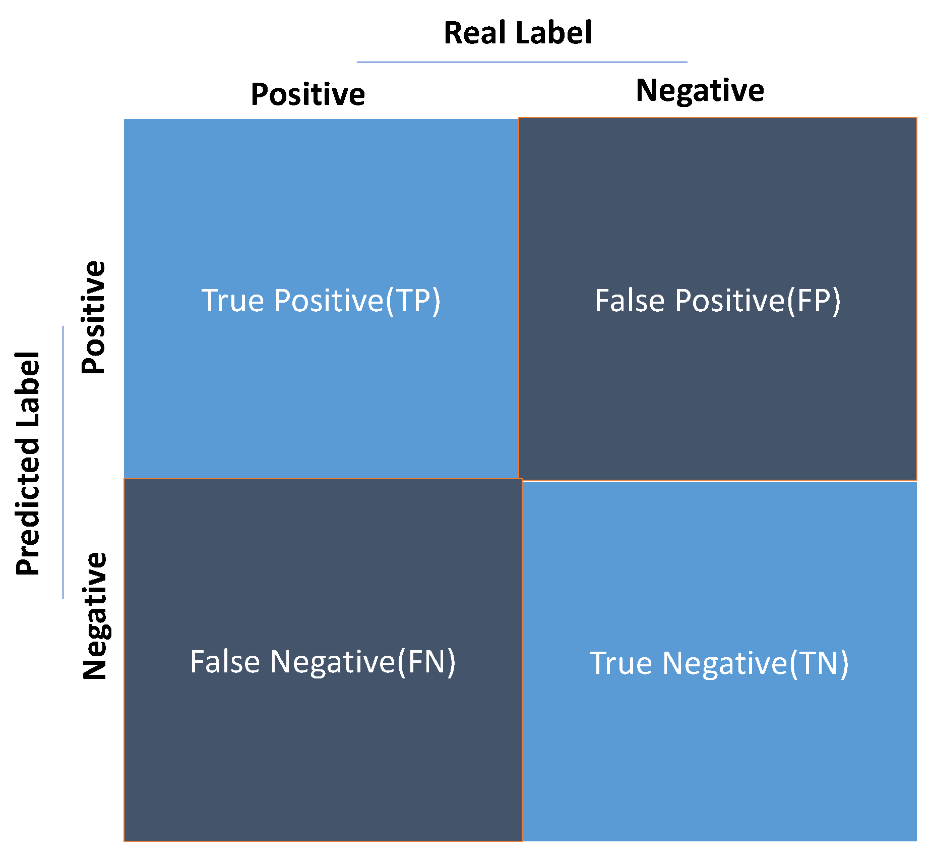
Table 1.
Evaluation Metrics for Classification: Including Threshold, Average, and Hybrid Metrics [56]
Table 1.
Evaluation Metrics for Classification: Including Threshold, Average, and Hybrid Metrics [56]
| Metrics | Formula | Evaluation Focus |
|---|---|---|
| Accuracy (acc) | Ratio of correct predictions over total instances. | |
| Error Rate (err) | Ratio of incorrect predictions over total instances. | |
| Sensitivity (sn) | Fraction of actual positives correctly classified. | |
| Specificity (sp) | Fraction of actual negatives correctly classified. | |
| Precision (p) | Positive patterns correctly predicted from total predicted positives. | |
| Recall (r) | Fraction of positive patterns correctly classified. | |
| F Measure (FM) | Harmonic mean of precision and recall. | |
| Geometric Mean (GM) | Balances true positive and true negative rates. | |
| Mean Square Error (MSE) | Measures difference between predicted and actual values. | |
| AUC | Overall ranking performance of a classifier. | |
| Optimized Precision (OP) | Hybrid metric combining accuracy, sensitivity, and specificity. | |
| OARP | Hybrid metric designed for classifier training. | |
| Averaged Accuracy | Average effectiveness across all classes. | |
| Averaged Error Rate | Average error rate across all classes. | |
| Averaged Precision | Average precision across all classes. | |
| Averaged Recall | Average recall across all classes. | |
| Averaged F Measure | Average F1 score across all classes. |
Table 2.
Agreement Metrics and Their Definitions
| Metric | Definition |
|---|---|
| Sensitivity () | Proportion of true positives correctly identified: |
| Specificity () | Proportion of true negatives correctly identified: |
| Raw Agreement (I) | Proportion of total agreement: |
| Agreement Due to Chance () | Expected agreement by chance: |
| Cohen’s Kappa () | Agreement corrected for chance: |
| Accuracy | Fraction of correct predictions: |
| Precision | Proportion of true positives among predicted positives: |
| Recall | Proportion of true positives correctly identified: |
| F1-Score | Harmonic mean of precision and recall: |
Disclaimer/Publisher’s Note: The statements, opinions and data contained in all publications are solely those of the individual author(s) and contributor(s) and not of MDPI and/or the editor(s). MDPI and/or the editor(s) disclaim responsibility for any injury to people or property resulting from any ideas, methods, instructions or products referred to in the content. |
© 2025 by the authors. Licensee MDPI, Basel, Switzerland. This article is an open access article distributed under the terms and conditions of the Creative Commons Attribution (CC BY) license (http://creativecommons.org/licenses/by/4.0/).
Copyright: This open access article is published under a Creative Commons CC BY 4.0 license, which permit the free download, distribution, and reuse, provided that the author and preprint are cited in any reuse.


