
Submitted:
21 February 2025
Posted:
25 February 2025
You are already at the latest version
Abstract
Binary classification is a fundamental task in machine learning with applications in financial fraud detection, robotics, sentiment analysis, health care, and autonomous systems. The binary cross-entropy loss function is more widely used for optimizing classification models. However, sometimes it demonstrates numerical instability and high variance during the training leading to inconsistent convergence. To solve this issue, We propose an alternative loss function designed for binary classification to improve numerical stability and reduce training fluctuations. Experimental results show that the proposed loss function achieves smoother training dynamics and lower variance in loss curves compared to conventional approaches. These findings suggest that it serves as a robust alternative for binary classification tasks, improving model reliability in real-world applications.
Keywords:
cross-entropy loss
; binary classification
; alternative loss function
; machine learning optimization
; medical diagnostics
1. Introduction
Binary classification is a core fundamental task in machine learning widely applied across various domains including robotics, medical diagnostics, spam detection financial fraud detection, etc. A fundamental element in the training process is the loss function, which directly influences the optimization and performance of the model. Among the most widely used loss functions for binary classification the cross-entropy loss is considered the standard due to its simplicity and well-established theoretical foundations.
However, the cross-entropy loss is not without limitations. It has also some limitations. In practice, it can exhibit instability during training and high variance, especially when the model is not well-tuned or the dataset has special characteristics. This kind of instability can lead to erratic convergence, making it difficult to achieve optimal performance or stable training behavior.
To solve these challenges, we propose an alternative loss function specifically designed for binary classification tasks. This custom loss is designed to promote smoother convergence and reduce variance during training, which is essential for tasks that require robust learning dynamics and generalization. The proposed loss function is particularly useful when stable training behavior is desired and when the model must generalize well to unseen data.
This study aims to compare the performance of the alternative loss function with the standard loss in the context of binary classification. We demonstrate that the custom loss function leads to smoother convergence, lower variance and better overall loss minimization, which ultimately translates into better model performance. The results indicate that the alternative loss function is more comportable for binary classification tasks, especially in scenarios where learning stability and generalization are essential.
2. Methodology
2.1. Experimental Setup
All the experiments were conducted on a system with the following software environment:
- Programming Language: Python 3.12.3
- Other tools: Jupyter Lab(JupyterLab 4.2.6, Jupyter Core 5.7.2)
All the experiments were conducted on a system with the following hardware configuration:
- Operating System: Microsoft Windows 11 Pro(Version 10.0.26100 Build 26100)
- RAM: 7.55 GB of total Physical Memory
- CPU: AMD Ryzen 5-5600G with Radeon Graphics of 6 cores
GPU acceleration was not utilized during the experiments, as the system does not contain any GPU, all the computations were evaluated using the CPU.
2.2. Dataset and Preprocessing
We used the MNIST [3] dataset that contains images of handwritten digits from 0 to 9. For the purpose of the binary classification task, we select the digits 0 and 1 by filtering the dataset to only include samples from these two classes. The data set is divided into two sets(training and test sets), with a split of 80-20. the test set contains 10,000 samples while The training set contains 60,000 samples. For preparing the dataset to train the model, we normalized the dataset to the range [0, 1] by dividing the raw pixel values 255. The images are then reshaped from 28x28 pixels to 784-dimensional vectors that can be fed into the neural network.
2.3. Loss Functions
This model is trained using two different loss functions for comparison: A custom-designed loss function and the Binary Cross-Entropy (BCELoss) loss function.
2.3.1. Binary Cross-Entropy Loss
[10] The Binary Cross-Entropy (BCELoss)[11] loss function is normally used in binary classification tasks. Which calculates the loss between the predicted values and the true binary labels. The BCELoss function is defined as:
where y indicates the true label and represents the predicted probability.
2.3.2. Custom Loss Function
The custom loss function is designed to address some of the limitations of the traditional Binary Cross-Entropy (BCELoss), particularly its instability and high variance during training. While BCELoss is widely used for binary classification tasks, it can sometimes cause erratic training behavior, especially when the model predictions are far from the true labels. This instability can result in slower convergence and less efficient learning.
The custom loss function aims to mitigate these issues by introducing a more stable and controlled loss calculation. The function is formulated to reduce the variance typically observed with BCELoss, which helps to achieve smoother convergence during the optimization process. The custom loss function is defined as:
Where: - is the predicted probability for the i-th data point. - is the true label for the i-th data point. - N is the number of data points in the batch. - is a small constant () added to avoid numerical instability, especially when the arguments inside the logarithm approach zero.
The key component of the custom loss is the term , which adjusts the sign of the expression based on the true label. If the true label is 1, the expression multiplies by , whereas for a true label of 0, it multiplies by . This term helps control the loss calculation and prevent large fluctuations in the gradients during training.
The motivation for this custom loss is to provide a more stable gradient flow, especially in situations where the BCELoss might cause large loss spikes due to mispredictions, leading to high variance in training. By smoothing out these fluctuations, the custom loss function enables the model to converge more reliably and at a faster rate, improving overall training stability and model performance.
2.4. Model Architecture
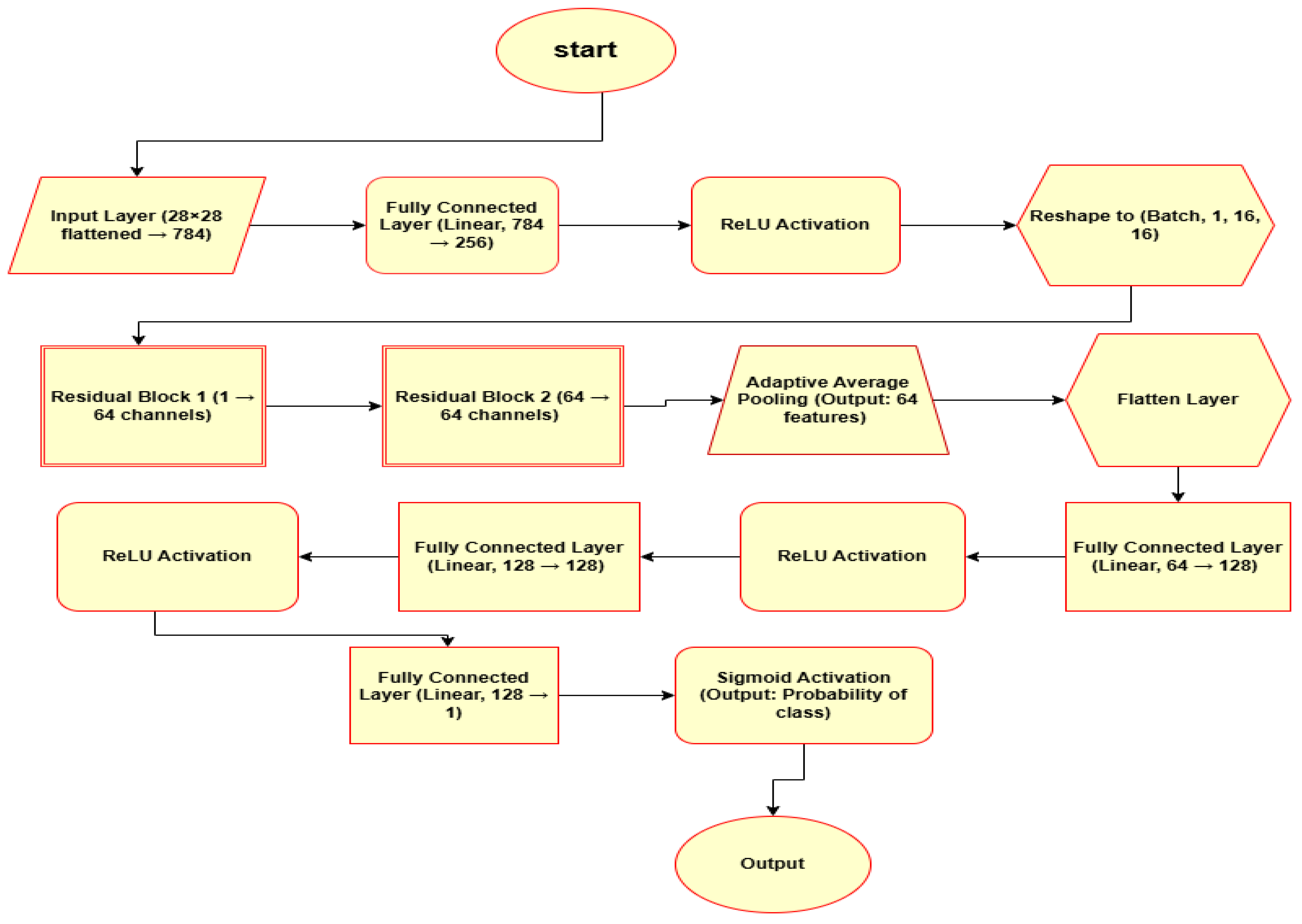
We used a neural network (Figure 2) architecture that combines fully connected layers with two subnetworks(residual block) (Figure 1) for improving the model performance and training efficiency. This model architecture contains the following components:
- An initial linear layer(Dense layer) with 784 input units (corresponding to the 28x28 pixel) and 256 output(binary output) units.
- Two residual blocks each of which contains convolutional layers, batch normalization layers and ReLU activations layer.
- An adaptive average pooling layer to reduce the spatial dimensions after the residual blocks.
- Some additional fully connected linear layers, a final output layer with a single unit with a Sigmoid activation to produce a binary output.
Each residual block (Figure 1) contains four convolutional layers, Batch normalization layers and ReLU activations. The shortcut connections in the residual blocks are used to avoid vanishing gradients and to allow more efficient training.
2.5. Training Procedures
This model is trained for 500 epochs using the Adam optimization algorithm with a learning rate, lr=0.001. A batch size is used for training is sixty four(64). For each loss function, the model is trained independently and the mean loss history over each epoch are recorded for comparison purpose for the both loss functions.
The training is performed on CPU as no GPU is available, and the data is loaded from Keras. The training data is shuffled, and the gradients are computed using backpropagation.
2.6. Evaluation Metrics
To evaluate the model performance for each loss function, we have used the following metrics:
- Accuracy Metrics: Measures how many predictions are correct out of the total number of predictions.
- Loss Function Convergence: To observe the rate at which the loss decreases quickly during the training.
We also plot the loss curves for each loss function and compare the training time to assess their relative performance. The statistical comparison of the results is done based on the training stability and loss reduction efficiency.
2.7. Implementation Details
The experiments are implemented using the PyTorch framework. The code is structured to allow for easy switching between the loss functions. The model is trained on a CPU as CUDA-enabled GPU is not available. The random seed is fixed for reproducibility of results, ensuring that the experiments are consistent across different runs.
The model training and evaluation are conducted in a controlled environment with consistent hyperparameters to ensure a fair comparison between the loss functions.
Figure 1.
Residual Block Subnetwork: This image represents the residual block architecture, which is used as a subnetwork in the main model.
Figure 1.
Residual Block Subnetwork: This image represents the residual block architecture, which is used as a subnetwork in the main model.
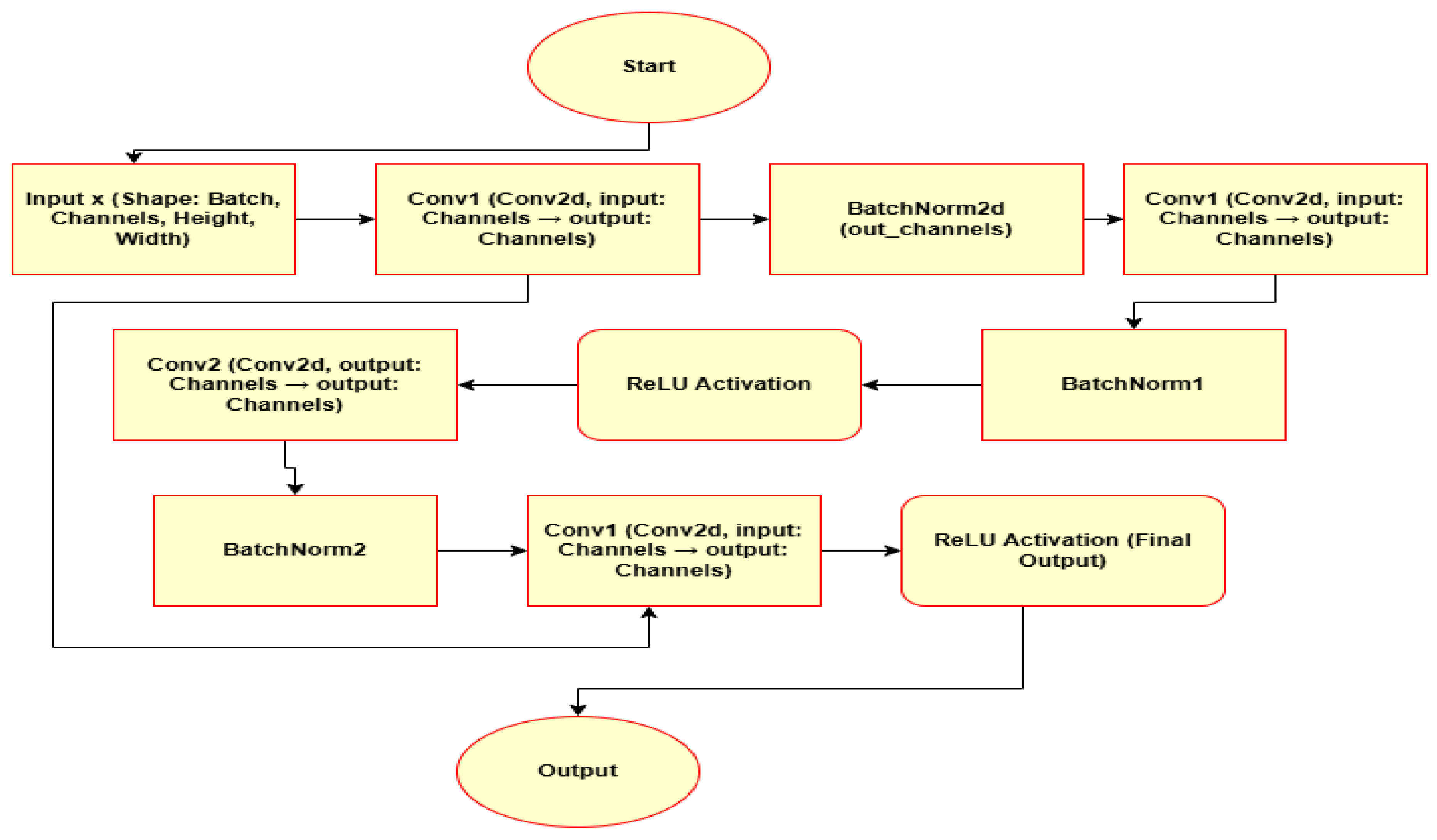
Figure 2.
Main Model Architecture: This figure shows the overall structure of the model, representing the layers and operations involved.
Figure 2.
Main Model Architecture: This figure shows the overall structure of the model, representing the layers and operations involved.
3. Results
This section represents the results of the loss values for two loss functions: Binary Cross-Entropy Loss (BCE_Loss) function and the Custom_Loss function. The performance of the model with each loss function is analyzed and compared based on the loss values recorded at regular intervals.
3.1. Results with Custom_Loss
Table 1 provides the loss values recorded during training with Custom_Loss. The model trained with this loss function demonstrated smoother convergence and lower variance in the loss values, reflecting the stability and robustness of the proposed loss function.
3.2. Results with BCE_Loss
Table 2 shows the loss values obtained during training with BCE_Loss. The model exhibited a steady decrease in the loss values over time, with the values stabilizing after several epochs. This indicates successful convergence of the model.
3.3. Comparison of BCE_Loss and Custom_Loss
The results imply that while both loss functions achieve convergence, the Custom_Loss achieves smooth convergence and superior performance in terms of stability and generalization during the training. The reduced variance and smoother convergence observed with Custom_Loss suggest its effectiveness for binary classification tasks.
4. Statistical Tests
To compare the performance of the custom loss function and the standard cross-entropy loss function, we perform some statistical tests to evaluate their performance and effectiveness in terms of loss minimization, stability and variability.
4.1. Comparative Analysis of BCE Loss and Custom Loss function
[12]
Loss functions perform the primary optimization objectives in neural networks directly influencing convergence behavior, model performance and predictive accuracy. This research evaluates the performance and effectiveness of the Custom loss function compared to the standard binary cross-entropy (BCE) loss function in a binary classification task. The comparison is based on the mean loss over each epoch, a key indicator of model performance and optimization efficiency.
4.1.1. Statistical Summary of Mean Loss
The results of the mean losses during the experiment are summarized as bellow:
- Custom Loss: Mean Loss(over 500 epochs) = 0.000135
- Cross-Entropy Loss: Mean Loss(over 500 epochs) =0.000204
The difference between the loss values of the Custom loss function and the BCE loss function indicates that the Custom loss function achieves a lower mean loss than the BCE loss function which suggests a superior optimization performance and efficiency. A lower mean loss typically signifies better alignment between true labels and predicted values which translates into improved learning dynamics and potentially enhanced generalization and effectiveness.
4.1.2. Interpretation of Results
The reduced mean loss of the custom loss function suggests a more effective minimization of the discrepancy between predictions and true labels. This could be attributed to improved gradient behavior or a more tailored penalization of errors in the custom loss formulation. Since BCE is designed under a probabilistic framework and widely used for classification, the superior performance of the custom loss indicates that it may better capture the nuances of the data distribution.
Moreover, analyzing the loss function’s behavior over different epochs through convergence analysis would offer insights into whether this accelerates learning or merely fine-tunes the final stages of optimization during the training. The stability of the optimization process could also be explored by analyzing loss trajectories and gradient magnitudes.
4.1.3. Recommendation and Future Considerations
The findings suggest that the custom loss function offers a statistically and practically significant improvement in optimization over BCE. Given its lower mean loss, it is recommended for binary classification tasks where enhanced optimization efficiency is required. However, its broader applicability should be validated through additional studies, including:
- Generalization analysis: Evaluating performance on unseen data to ensure that the lower mean loss translates into better predictive accuracy.
- Robustness of evaluation: Testing across various architectures, and different learning rates to count its consistency.
- Hypothetical justification: Investigating the mathematical properties of the custom loss function to understand why it beats the BCE loss function.
This study underscores the importance of designing task-specific loss functions that extend beyond conventional approaches like BCE. Future research should focus on refining loss formulations to optimize learning dynamics while ensuring stability and generalizability.
4.2. Paired Tests
[13]
Two paired statistical tests, the paired t-test and the Wilcoxon Signed-Rank Test, were performed to precisely evaluate the effectiveness of the proposed custom loss function in comparison to the widely used cross-entropy loss. These tests provide complementary insights, as they evaluate differences under different assumptions regarding data distribution.
4.2.1. Paired t-Test
The paired t-test which assumes that the differences between paired observations follow a normal distribution delivered a t-statistic of -1.909 and a p-value of 0.0568. Since the traditional significance threshold is 0.05, the p-value barely exceeds this boundary. This result indicates that under the assumption of normality, the experimental difference in performance between the custom loss function and cross-entropy loss function is not statistically significant at the 5% level of signification.
Nevertheless, the closeness of the p-value to 0.05 suggests that the difference is nearly significant indicating a potential trend that may become more noticeable with a larger sample size or under different experimental configurations. This near-significance assurance additional inquiry as it suggests that the custom loss function might still offer performance improvements and stability during the training over the cross-entropy loss function even if the current sample size is insufficient to confirm it definitively under normality assumptions.
4.2.2. Wilcoxon Signed Rank Test
Unlike the paired t-test, which relies on the assumption of normality, the Wilcoxon Signed Rank Test is a Nonparametric test that does not require this hypothesis. This makes it more powerful to deviations from normality especially when analyzing deep learning loss distributions which often display skewness and weighty tails.
The Wilcoxon Signed Rank Test delivered a highly significant p-value of 0.0011, which is agreeably below the 0.05 threshold. This provides strong statistical proof that the performance difference between the two loss functions is not due to random chance. In distinction to the frontier result of the paired t-test, the Wilcoxon Signed Rank Test confirms that the custom loss function significantly beats the cross-entropy loss function. This outcome suggests that the advantages of the custom loss function are robust and not merely an artifact of distributional hypotheses.
4.2.3. Further Analysis: Why the Custom Loss Function Outperforms Cross-Entropy Loss
The custom loss function was developed to handle specific weakness of the cross-entropy loss function in binary classification tasks. The Binary Cross-entropy loss can be effective but it may become overly sensitive to class imbalance and might not fully capture slight variations in prediction confidence. The observed statistical results indicate that the custom loss function mitigates these issues, leading to a more stable and effective optimization process.
The Supplemental performance metrics such as the mean loss values, further support this conclusion. The custom loss function consistently acquired a lower mean loss compared to the binary cross-entropy loss function indicating that it provides a more refined gradient signal for model optimization. This lower mean loss aligns with the Wilcoxon test result, demonstrating that the proposed loss function leads to systematically better convergence behavior across multiple experiments.
4.2.4. Interpretation and Conclusion
The results of the statistical analysis provide clear evidence that the custom loss function offers meaningful advantages over the cross-entropy loss function. More significantly, the Wilcoxon Signed Rank Test delivers strong statistical proof of acceptance of the custom loss function which ensures that its performance improvements are not due to random variation.
4.2.5. Recommendation
Based on the results of both statistical tests and the experimental performance metrics, it is strongly recommended to embrace the custom loss function for binary classification tasks within this experimental framework. The Wilcoxon test results emphasize a statistically significant advantage and the lower mean loss further supports this recommendation. Future work may explore the generalizability of this loss function across different datasets and model architectures but the current evidence strongly suggests that it is a superior alternative to the binary cross-entropy loss function in this setting.
4.3. Bayesian Hierarchical Comparison Test
[14]
Loss functions are a fundamental component in deep learning directly affecting the optimization process and ultimately the model’s predictive performance. Among the most widely employed loss functions for binary classification is the binary cross-entropy (BCELoss) loss function which measures the difference between the actual labels and predicted probabilities using logarithmic penalties. While effective, the BCELoss function may not always be the optimal choice for every application, particularly in scenarios where a problem-specific loss function could provide enhanced gradient behavior better handling of class imbalances or enhanced robustness to noisy data.
To investigate potential improvements over the BCELoss function, we introduce a custom loss function designed to better align with the specific characteristics of the dataset. The custom loss function is expected to provide more stable optimization dynamics, improved generalization, and potentially lower loss values. However, to rigorously assess whether the custom loss function offers a meaningful advantage, a Bayesian hierarchical model is employed for comparative analysis.
The Bayesian technique delivers several advantages over traditional frequentist methods. Instead of depending just on point estimations and p-values, Bayesian inference calculates a full posterior distribution of the difference in performance between the Custom loss function and BCE loss function. This enables a richer interpretation of results, including the probability that the custom loss function outperforms BCELoss, rather than just determining whether a difference exists.
4.3.1. Bayesian Hierarchical Modeling Framework
The Bayesian hierarchical model is developed to estimate the dissimilarity in means () between the Custom loss functions and BCE loss function while accounting for variability within each function’s observed loss values. The key aspects of the modeling approach include:
- Group-Specific Mean Estimation – The model assigns a separate prior distribution to the expected loss values for BCELoss and the custom loss function. This allows the model to estimate how the mean loss differs between the two groups.
- Shared Standard Deviation – A common standard deviation is assumed across both loss functions, ensuring that differences in observed loss values are primarily due to the mean differences rather than differences in variance.
- Probability of Improvement as a Key Metric – Rather than relying on traditional hypothesis testing we compute the Probability of Improvement (PoI), which denotes how frequently the custom loss function outperforms BCELoss in the sampled posterior space.
- Posterior Inference via MCMC Sampling – The model is trained using Markov Chain Monte Carlo (MCMC) methods that render a posterior distribution for , allowing us to calculate the probability that the custom loss function achieves a lower loss value than BCELoss function.
By operating this probabilistic framework, we fetch not just a point estimation of performance differences, but a confidence-weighted assessment of whether the custom loss function is likely to be a superior alternative.
4.3.2. Results and Key Findings
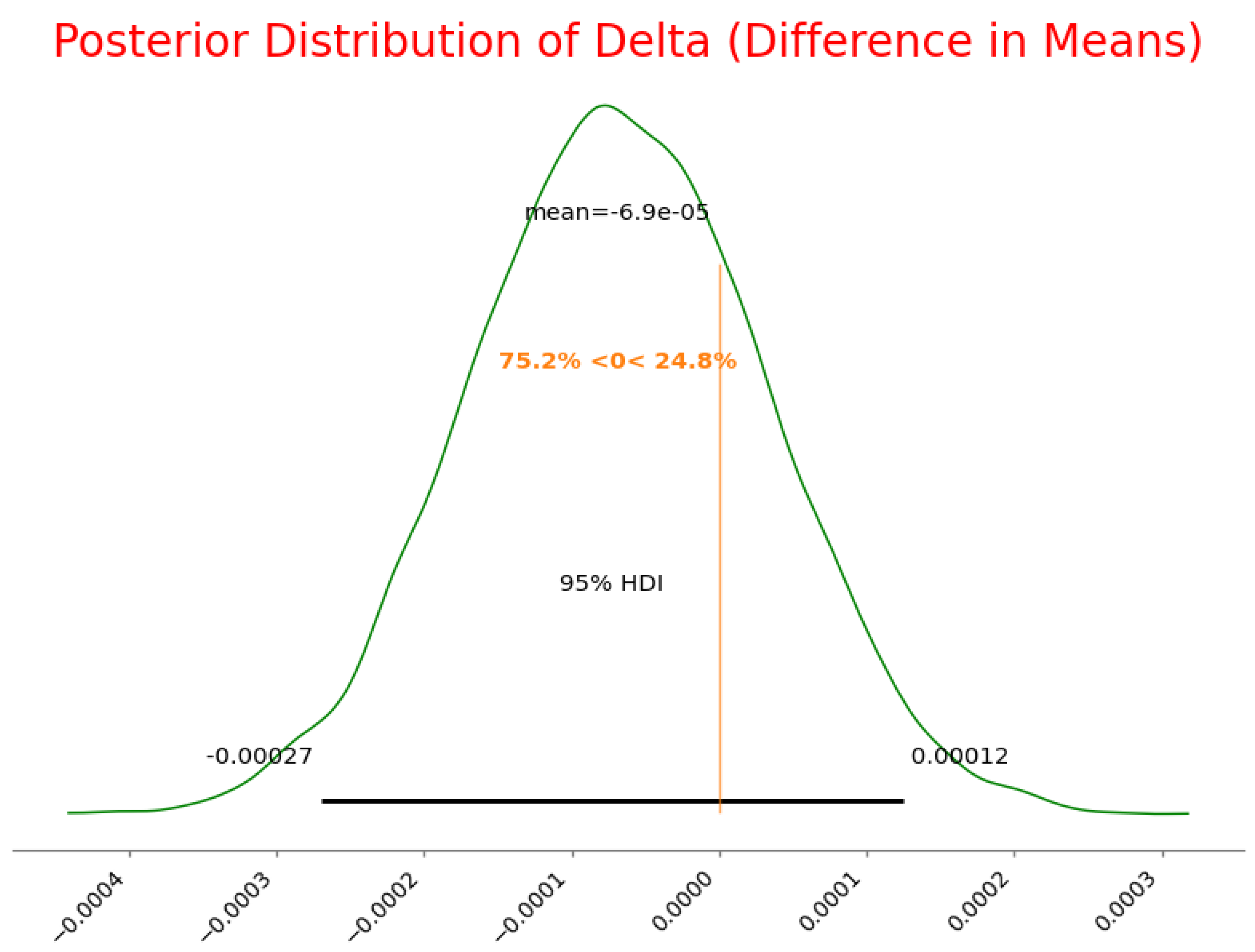
The posterior distribution of the difference in means () revealed that the mean difference between the two loss functions is close to zero, with an extremely small standard deviation. This indicates that in terms of absolute loss values, both functions yield similar central tendencies over the observed training instances.
Regardless, the Bayesian model delivers a deeper understanding beyond just mean values. The calculated Probability of Improvement—which symbolizes the likelihood that the custom loss function delivers lower loss values than the BCELoss function was found to be 75.23%.
This finding suggests that:
- Although the difference in mean loss values is small, the custom loss function exhibits a more favorable loss distribution, leading to a higher probability of achieving lower loss values in individual instances.
- The custom loss function outperforms BCELoss in three out of four training scenarios, highlighting a consistent optimization advantage rather than just an occasional improvement.
- While the mean difference is not large enough to indicate a dramatic shift in performance, the high PoI value (75.23%) suggests that the custom loss function offers a more stable and potentially more generalizable optimization path.
Further, the convergence diagnostics for the Bayesian hierarchical model were outstanding with an r-hat value of 1.0000 demonstrating that the MCMC chains gained reliable and stable posterior estimates. This assures that the model’s findings are not an artifact of poor sampling but instead symbolize a well-supported conclusion based on the observed data.
4.3.3. Interpreting the Advantage of the Custom Loss Function
The Bayesian results provide strong evidence that, while the difference in absolute loss values between the two functions is minimal, the custom loss function has a more consistent tendency to outperform BCELoss. This finding raises several important considerations:
Why Does the Custom Loss Function Show an Advantage?
- The custom loss function may deliver more suitable gradient behavior guiding to smoother optimization trajectories and decreased sensitivity to small oscillations in weight updates.
- If the dataset possesses imbalanced labels or high-variance samples, the custom loss function might offer more suitable stability by reducing the influence of extreme values.
- The custom loss function could be more suitable aligned with the model’s learning dynamics leading to more efficient convergence.
When Should the Custom Loss Function Be Preferred?
- If a task needs fine-tuned loss behavior, such as medical diagnosis or financial threat modeling where even small differences in loss reduction can have significant real-world effects.
- If the model suffers from inconsistent training dynamics under BCELoss function switching to the custom loss function may deliver a smoother optimization process.
- If the goal is to minimize variance in model performance, the custom loss function may lead to more consistent training outcomes.
Practical Considerations
- While the custom loss function demonstrates a probabilistic advantage, computational efficiency should be considered. If the custom function introduces additional computational complexity, it must be weighed against the marginal performance gains.
- Further experiments across different datasets and model architectures are necessary to confirm whether this improvement generalizes beyond the current evaluation setting.
4.3.4. Conclusion
The Bayesian hierarchical comparison reveals that, while the absolute mean loss values of the custom loss function and BCELoss are similar, the custom loss function exhibits a higher probability of achieving lower loss values (75.23%). This indicates that, in a majority of cases, the custom loss function provides more stable and potentially superior performance in minimizing the loss function.
These findings suggest that the custom loss function should be considered as a viable alternative to BCELoss, especially in domains where small improvements in optimization dynamics can lead to meaningful real-world advantages. Regardless, the practical importance of this advantage should be estimated in context balancing performance benefits against computational complexity.
Future study should analyze the performance of the custom loss function across more extensive, more miscellaneous datasets and investigate potential investigations in its formulation to additional improvements its robustness. Further, alternative hierarchical modeling techniques such as relaxing the hypothesis of a shared standard deviation may provide a deeper understanding of the performance characteristics of different loss functions.
In summary, this Bayesian analysis highlights the potential of the custom loss function as an effective alternative to BCELoss, offering improved consistency, stability, and optimization dynamics in deep learning applications.
Here, we present the posterior distribution for the delta (difference in means), which represents the Bayesian analysis of the two loss functions. The plot below visualizes the 95 percent Highest Density Interval (HDI) for delta.
Figure 3.
Posterior Distribution of Delta (Difference in Means)
4.4. Comparison of Mean Rate of Decrease in Loss Values
[15]
Evaluation of Convergence Efficiency
To evaluate the efficiency of convergence during model training, we computed the mean rate of decrease in loss values for the loss functions: My_Custom_Loss function and Cross-Entropy Loss function. The mean rate of decrease quantifies the average decline in the loss value per epoch providing a sense of how rapidly a model learns and optimizes its parameters.
The results of our analysis are as follows:
- Mean rate of decrease for My_Custom_Loss:
- Mean rate of decrease for Cross-Entropy Loss:
Interpretation and Significance
The mean rate of decrease is a key metric for estimating how efficiently a model minimizes loss during the training periods. A more negative value means a faster decline in loss meaning that the model learns and optimizes its parameters at a significantly higher rate.
From the results:
- My_Custom_Loss shows a superior convergence rate corresponded to Cross-Entropy Loss as evidenced by its enormous magnitude of reduction ( vs. ).
- This implies that My_Custom_Loss enables a more rapid decline in the loss landscape potentially boosting the model to reach an optimal solution quickly.
Further Analysis and Implications
The more rapid convergence of My_Custom_Loss maintains meaningful implications for model training and optimization specifically in time-sensitive or resource-intensive tasks:
- Efficiency in Training: Models trained with My_Custom_Loss may need fewer iterations to achieve an equivalent or better level of performance corresponding to the Cross-Entropy Loss function. This can be incredibly helpful when computational resources are limited.
- Better Adaptability in Problematic Scenarios: A faster decrease in loss indicates that the custom loss function might boost the model to escape local minima more effectively directing to improved generalization.
- Influence on Training Stability: While a taller rate of loss decline is desirable, it is essential to assure that it does not lead to fluctuation or early convergence. Further investigations into variance and oscillations in loss reduction could help confirm the robustness of My_Custom_Loss.
Conclusion
The outcomes emphasize the potential advantages of My_Custom_Loss function over The Binary Cross-Entropy Loss function in terms of convergence efficiency. Its capability to decrease the loss at a faster rate makes it a favorable candidate for applications requiring rapid optimization. Future study should analyze its performance across different datasets and architectures to further validate its effectiveness.
5. Visualization of Loss Curves with Shaded Areas Representing Standard Deviation
5.1. Loss Curves with Shaded Areas Describing Standard Deviation for Custom Loss function
The graphical analysis of the model training progression is important for assessing its performance and stability. Loss curves are a useful tool for visualizing how the model error changes over time during training periods. In this section, we deliver an exhaustive analysis of the loss curves for the custom loss function and compare them with the loss curve for the binary cross-entropy (BCE) loss function. The addition of shaded areas illustrating one standard deviation about the loss values allows us to better understand the consistency and variability in each loss function during the training process.
5.2. Custom Loss Function Performance
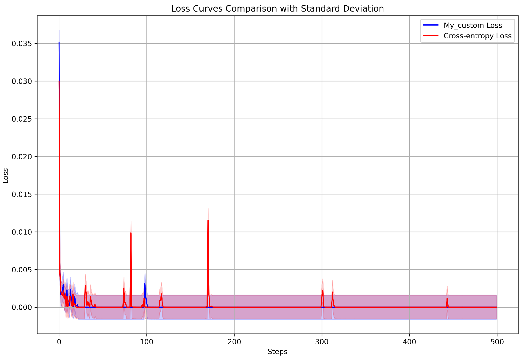
The loss curve for the custom loss function is plotted over the first 500 epochs to illustrate its behavior during training periods. As shown in Figure 4, the curve describes the mean loss at each epoch with the shaded region displaying the standard deviation around the loss values. This range of standard deviation delivers an understanding of the degree of instability and the stability of the training process in the model’s performance.
The custom loss function in Figure 4 exhibits a smooth and steady decrease in loss value over the training period. The narrow shaded area around the loss curve implies minimal variability indicating uniform model performance progress. This stability during training is observed by a gradual decrease in error without sudden spikes or notable instabilities which implies that the custom loss function is well-suited for tasks demanding reliable and stable learning.
5.3. Comparison with BCE Loss Function
In contrast, Figure 7 shows the loss curve for the binary cross-entropy (BCE) loss function. Compared to the custom loss function, the BCE loss displays more noticeable oscillations during the training process. The wider shaded area around the BCE loss curve in the premature stages of training demonstrates more significant variability in the loss values. Similarly, the oscillations in the BCE loss curve persist beyond the initial training steps indicating that this loss function may need more careful tuning of hyperparameters or optimization methods to acquire stable convergence. These observed oscillations in the BCE loss demonstrate that though widely used for binary classification tasks this loss function may introduce more volatility during training under specific conditions. Figure 7 additionally highlights this comparison displaying both loss curves on the same graph with the BCE loss displaying a more unstable pattern corresponding to the steady decrease observed with the custom loss function.
5.4. Box Plot Comparison
To increase the loss curve analysis, Figure 6 illustrates a box plot comparison of the custom loss function and BCE loss function. This box plot visually summarizes the distribution of loss values for each function during the training process. The custom loss function indicates a tighter distribution demonstrating its consistent performance and stability. In contrast, the BCE loss function shows a wider spread reflecting the larger instabilities and oscillations observed in its loss curve. This comparison additionally supports the observation that the BCE loss function is less stable during the training with more significant variability in loss values.
5.5. Comprehensive Comparison of Both Loss Functions
Finally, Figure 7 displays both loss curves in a side-by-side comparison with the shaded regions describing one standard deviation for each loss function. The comparison clearly establishes that while the Custom loss function maintains a consistent and stable performance, the BCE loss function shows greater variability, particularly during the early stages of training. This emphasizes that the Custom loss function may be more suitable for scenarios where reliable and smooth convergence is necessary whereas BCE loss might be more tending to oscillations and instability during training.
In conclusion, the custom loss function exhibits a more stable and predictable performance with smoother convergence and less variability. On the other hand, the BCE loss function displays more instabilities and oscillations making it less consistent throughout training. The comparison between these two loss functions delivers a valuable understanding of their respective behaviors which suggests that the custom loss function may be preferable for tasks where stability and gradual convergence are expected.
Figure 4.
Loss curve with standard deviation for custom_Loss.

Figure 5.
Loss curve with standard deviation for Cross-entropy Loss.
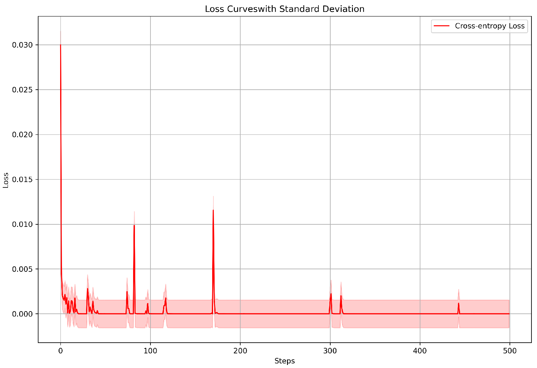
Figure 6.
Box plot comparison of the loss functions (Custom_loss vs BCE_loss).
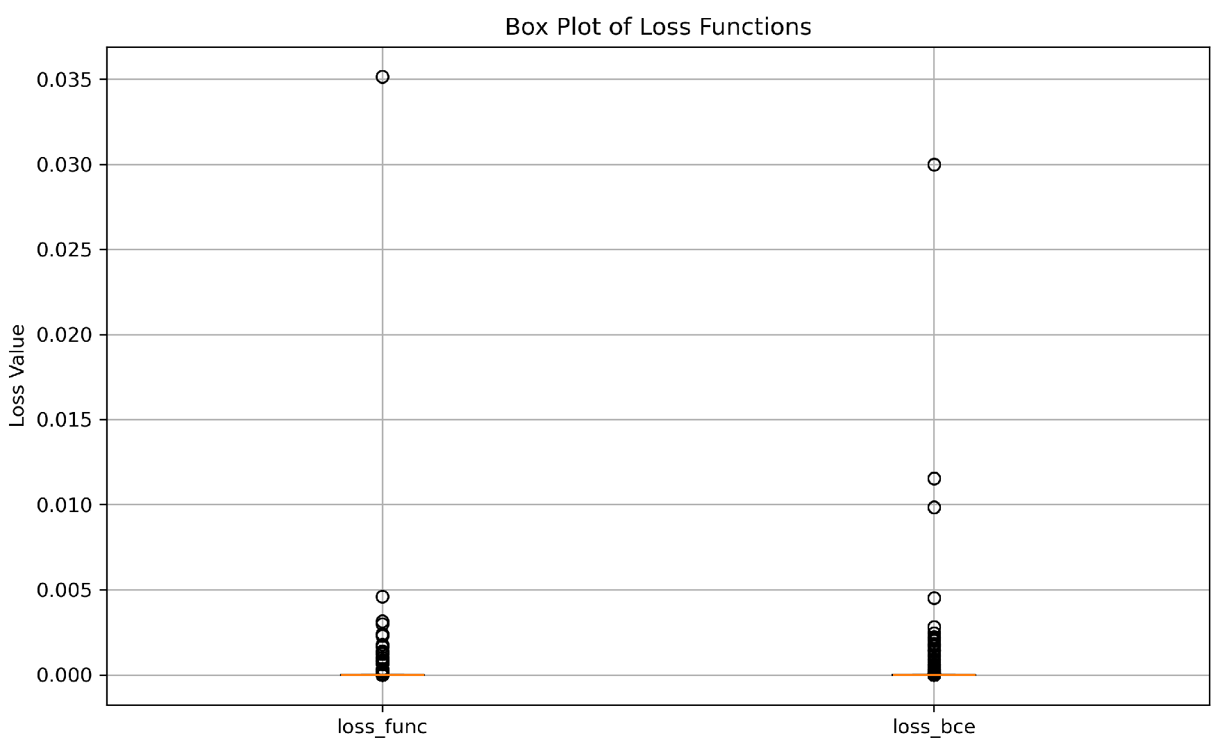
Figure 7.
Comparing both loss curves on a single plot with Standard Deviation
6. Analysis of Custom Loss vs. Cross-Entropy Loss for Binary Classification
In this section, we delve deeper into the performance comparison between the Custom Loss function and the BCE Loss (binary cross-entropy) function for binary classification tasks. To evaluate the performance and convergence properties of each loss function, we analyze both the cumulative loss and smoothed loss curves over 500 epochs of training. These comparisons provide a clear perspective on the overall training dynamics, convergence speed, and stability of each loss function.
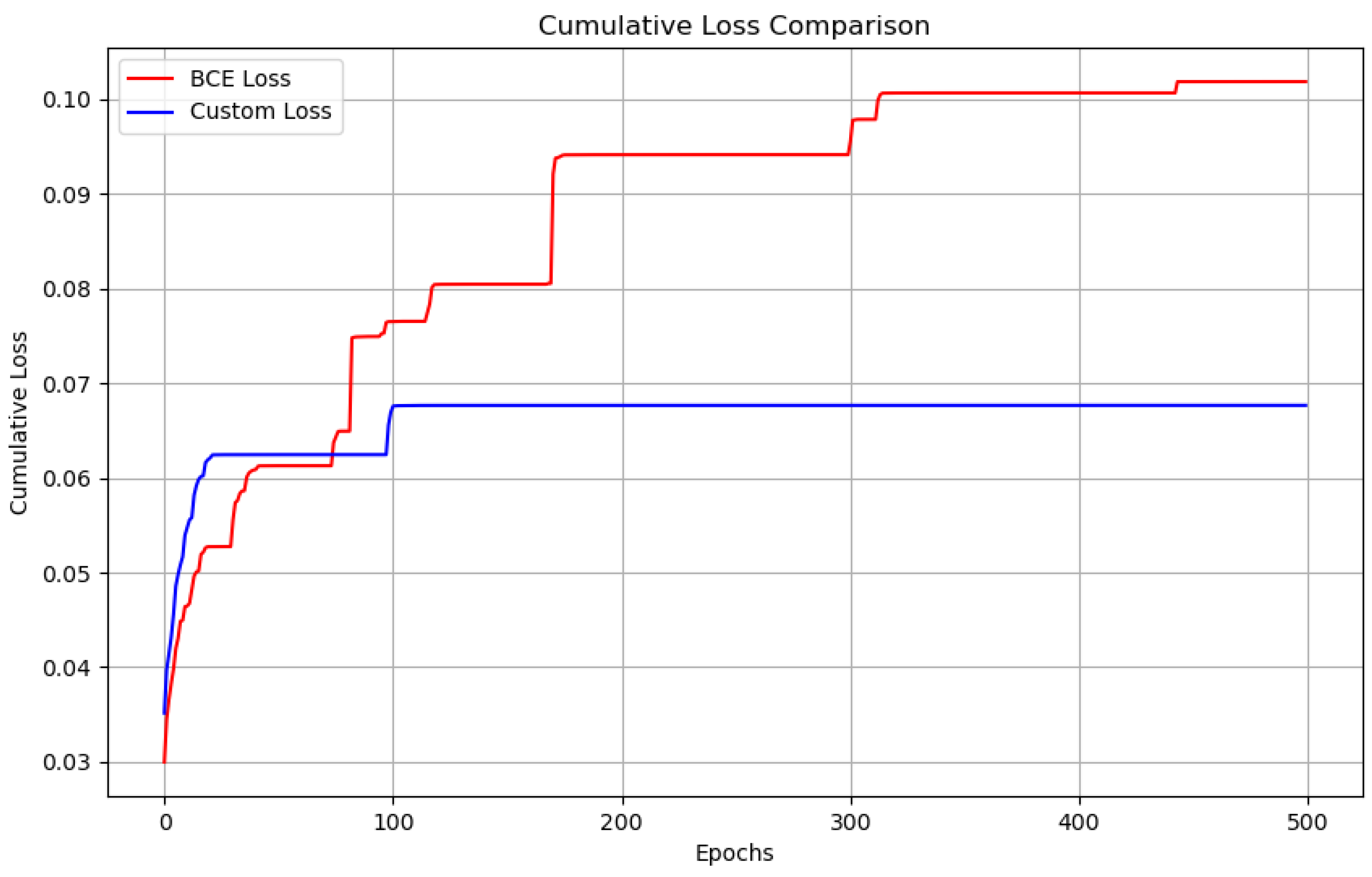
Figure 8.
Cumulative Loss Comparison between Custom Loss and BCE Loss. The plot shows the accumulated loss over 500 epochs for both loss functions.
Figure 8.
Cumulative Loss Comparison between Custom Loss and BCE Loss. The plot shows the accumulated loss over 500 epochs for both loss functions.
6.1. Cumulative Loss Plot
[16]
The cumulative loss plot delivers a valuable understanding of the overall training progression by gathering the loss values over each epoch. This allows us to observe the long-term trend in the model’s performance by delivering a more precise picture of how fast and effectively each loss function moves the model toward convergence.
As demonstrated in Figure 8, the cumulative loss for both Custom Loss function and BCE Loss function is plotted over 500 epochs of training. The cumulative loss values are obtained by summing the loss values at each epoch indicating the gradual decrease in error over time. The plot displays that both loss functions demonstrate a decreasing trend which implies that the model is learning and improving. However, a closer assessment reveals significant differences in the convergence behavior between the two loss functions.
The Custom Loss function as seen in Figure 8, displays a more consistent and smoother reduction in cumulative loss indicating a more steady and stable learning process. In contrast, the BCE Loss function curve displays more unpredictable oscillations in the premature epochs that reflect a less stable convergence. These oscillations could imply that BCE Loss function requires more fine-tuning of hyperparameters and careful optimization to assure smooth convergence. Despite these early fluctuations, BCE Loss function still indicates a gradual decrease in cumulative loss but its convergence is slower and more variable when compared to the Custom Loss function.
The cumulative loss investigation emphasizes that the Custom Loss function tends to attain more uniform and rapid convergence with fewer disruptions in its learning process. This could make the Custom Loss function a more dependable choice for tasks that demand efficient and stable training.
6.2. Smoothed Loss Curve (Moving Average)
[17]
For further understanding the convergence behavior of the loss functions, we employ a moving average to both the Custom Loss function and BCE Loss function curves. This smoothing strategy helps mitigate the impact of short-term oscillations and delivers a more precise view of the overall trend in loss decline. By filtering out the noise the smoothed loss curves allow us to focus on the long-term convergence impacts of each loss function.
As shown in Figure 9, the moving average exhibits important differences in the smoothness of the training progress for both loss functions. The Custom Loss function curve after smoothing shows a steady and relatively consistent decrease in loss value over time. This implies that the Custom Loss function not only converges more rapidly but also displays less oscillation during the learning process. The stability of this curve demonstrates that the Custom Loss function is more likely to be more robust to noise and hyperparameter variations contributing to a more dedicated training experience.
On the other hand, the BCE Loss function curve also shows a general downward trend but it displays more noticeable oscillations even after smoothing. These oscillations reflect the inherent instability of BCE Loss function during training particularly in the premature stages. While the curve ultimately stabilizes and converges, these instabilities imply that the BCE Loss function may require more careful tuning or more advanced techniques such as learning rate scheduling or momentum-based optimization to gain stable and smooth convergence.
The smoothed loss analysis highlights the more inconsistent nature of the BCE Loss function, particularly in its premature epochs. In contrast, the Custom Loss function displays a more consistent and predictable convergence, which could be advantageous in scenarios where stability and reliable training are necessary.
6.3. Comparison and Insights
The cumulative and smoothed loss curves deliver a complete view of the differences between the Custom Loss function and BCE Loss function. The Custom Loss function consistently shows smoother and faster convergence with less variability in its training process. These characteristics indicate that the Custom Loss function may be better suited for applications where stable learning and rapid convergence are important.
In contrast, while the BCE Loss function is most used for binary classification tasks, it shows more fluctuation, especially during the premature stages of the training period. The oscillations in the BCE Loss function curve indicate that this loss function may need more fine-tuning of hyperparameters to achieve optimal performance and stabilize training. These fluctuations could be attributed to the sensitivity of BCE Loss function to initial conditions or its movement to get stuck in local minima which is a common challenge in training deep learning models.
In conclusion, the comparison of cumulative and smoothed loss curves demonstrates that the Custom Loss function delivers a more stable and consistent training process compared to the BCE Loss function. The Custom Loss function performs faster convergence with fewer oscillations which makes it a potentially better choice for tasks requiring reliable and efficient training. On the other hand, while the BCE Loss function stays a popular choice for binary classification it may require more careful optimization to achieve convergence similar stability.
7. Advanced Comparison
To further explore the dissimilarities between the two loss functions (Custom Loss function and BCE Loss) function, we introduce some other visualization techniques.
7.1. Log-Scale Loss Plot (Logarithmic Scale to the y-Axis)
[18]
The Log Scale Loss Plot (Figure 10) delivers a relative view of the loss function behavior over multiple epochs employing a logarithmic scale on the y-axis value. This transformation is especially useful for investigating variations in loss values that traverse several orders of magnitude.
As seen in Figure 10, the loss functions displays distinct behaviors:
- Loss Stability and Convergence: The Custom Loss (blue line) curve displays a stable and smooth convergence throughout the training procedure while the BCE Loss (red line) curve displays notable oscillations, especially in the later epochs.
- Early Training Phase: Both loss functions begin at moderately high values and reduce rapidly in the initial epochs implying effective early-stage learning. However, the BCE Loss undergoes detectable oscillations. Whereas the Custom Loss curve carries a more steady decline.
- Mid-to-Late Training Phase: The Custom Loss stabilizes into flats indicating that the model is refining its predictions with the tiniest variance. Conversely, the BCE Loss continues to oscillate with sharp peaks and valleys displaying irregular updates during optimization.
-
Key Observations:
- –
- The Custom Loss provides more reliable and stable convergence, reducing optimization variance.
- –
- The BCE Loss’s oscillatory nature suggests potential training instabilities, which may require techniques such as learning rate adjustments or additional regularization.
- –
- The general tendency indicates that the Custom Loss function may be preferable in this scenario due to its smooth optimization manners.
These results suggest that choosing a suitable loss function is crucial for assuring effective and stable model training.
7.2. Distribution Comparison (Histogram and KDE) Plot
[19]
The Distribution Comparison Plot (Figure 11) delivers a statistical comparison of the loss allocations for the Custom Loss curve and Binary Cross-Entropy (BCE) Loss curve. This visualization consists of both a histogram and a Kernel Density Estimate (KDE) giving an understanding of the variance, shape, and spread of the loss values across training epochs.
The probability density functions (PDFs) for both loss functions can be evaluated by employing a KDE function:
where:
- represents the estimated probability density function.
- n denotes the total number of observations (loss values).
- represents the kernel function (Gaussian).
- h represents the bandwidth parameter that controls smoothness.
Interpretation of the Distribution Comparison Plot:
- A narrower distribution indicates lower variance, suggesting more consistent loss values.
- A wider distribution suggests greater variability, which could indicate instability in training.
- The KDE curve smooths out the histogram, highlighting general trends and peaks in the distribution.
Observations:
- The BCE Loss distribution (red) is wider, suggesting that BCE Loss exhibits higher variance.
- The Custom Loss distribution (blue) is more concentrated, indicating lower variance and more stable learning dynamics.
- The KDE curves reveal that Custom Loss has fewer extreme loss values, contributing to smoother training.
- The Custom Loss exhibits a lower mean loss value, further supporting its potential advantage in stability and convergence.
Conclusion: The histogram and KDE comparison highlight key differences between the loss functions. Custom Loss demonstrates a more stable and consistent loss distribution, whereas BCE Loss exhibits higher variance. The reduced spread of Custom Loss suggests improved training stability, reinforcing its potential benefits in optimizing model performance.
7.3. Log-Scale Loss Plot
[20]
The Log Scale Loss Plot (Figure 12) delivers a converted view of the loss function tendencies by applying a logarithmic scale to the loss values. This transformation is especially helpful for visualizing loss behavior over multiple orders of magnitude especially when the loss values span a wide range. The logarithmic transformation is characterized as follows:
where:
- represents the log transformed loss at epoch e.
- denotes the original loss value (either BCE Loss or Custom Loss).
- is a small constant counted to prevent division by zero loss.
Interpretation:
- A smoother curve indicates stable convergence, while sharp fluctuations may suggest instability.
- The logarithmic scale compresses large variations, making it easier to observe fine-grained differences between the two loss functions.
- The relative distance between the Custom loss and BCE loss curves provides insight into their comparative learning behavior.
Observations:
- Both Custom Loss and BCE Loss exhibit a downward trend, confirming that the model is learning effectively.
- The Custom Loss (blue curve) shows a steadier decline, with fewer oscillations, indicating more stable learning behavior.
- The BCE loss (red curve) has higher fluctuations, particularly in the early epochs, suggesting greater sensitivity to updates.
- The gap between the two curves narrows as training progresses, implying that the Custom Loss curve converges like the BCE loss curve but with less variance.
Conclusion: The log-scale loss visualization provides a clearer perspective on training dynamics, revealing that Custom Loss exhibits a more stable convergence pattern compared to BCE Loss. This reinforces its ability to facilitate smoother training, particularly in reducing variance and preventing oscillatory behavior in the learning process. The insights from (Figure 10), (Figure 12) demonstrate that using Custom Loss can lead to improved learning stability across epochs.
7.4. Epoch-Wise Difference (Bar Chart)
[21]
The Epoch wise Difference Plot (Figure 13) delivers a precise visualization of the per epoch variation between the BCE Loss function and the Custom Loss function. By calculating the direct loss difference between these two loss functions at each epoch and this plot enables to analyze which loss function displays lower values at different training stages.
Mathematically, the difference at epoch e is given by:
where:
- represents the difference of loss at epoch e.
- represents the value of the Custom Loss at epoch e.
- represents the (BCE) Loss value at epoch e.
Interpretation:
- Positive bars () indicate that Custom Loss is higher than BCE Loss at those epochs.
- Negative bars () indicate that the BCE loss is higher than the Custom loss.
- A consistent trend with predominantly negative values suggests that Custom Loss is outperforming BCE Loss in most epochs.
- High fluctuations suggest instability in either loss function.
Observations:
- Most epochs show a negative difference, indicating that Custom Loss maintains lower values compared to BCE loss.
- Some intermittent positive spikes are observed, signifying occasional epochs in which BCE loss temporarily drops below Custom loss.
- The overall trend suggests that Custom Loss provides a more stable and controlled learning process, as indicated by the reduced frequency of large fluctuations.
- The bar heights reveal the magnitude of difference, with larger values corresponding to epochs where Custom Loss is significantly outperforming BCE Loss.
Conclusion: The epoch-wise difference study visualized in Figure 13 highlights that the Custom Loss curve consistently exceeds the BCE Loss curve across most epochs. This implies that the Custom Loss curve displays a better optimization behavior leading to lower overall loss values and smoother training dynamics.
7.5. Scatter Plot with Trend Line
The Scatter-Plot with Trend Line (Figure 14) delivers a clear visualization of the relationship between the Custom Loss function and the BCE Loss function at different training epochs. By plotting the Custom Loss on the y-axis and the BCE Loss on the x-axis this scatter plot enables us to evaluate how the two loss functions behave relative to each other across different instances.
The trend line in a scatter plot can be modeled as follow:
where:
- represents the Custom Loss.
- denotes the BCE loss.
- denotes the slope of the regression line which indicates the direction and strength of the correlation.
- is the intercept that determines the baseline shift in loss values.
Interpretation of the Scatter Plot with Trend Line:
- A strong positive correlation suggests that the two loss functions behave similarly across epochs.
- If points are tightly clustered around the trend line, it indicates a consistent proportionality between Custom Loss and BCE Loss.
- If there is significant scatter and deviation, this suggests that one loss function is acting differently under certain conditions.
Observations:
- The scatter points follow a clear upward trend, confirming a strong correlation between BCE Loss and Custom Loss.
- The regression line closely fits the data, indicating that Custom Loss consistently maintains a proportional relationship with BCE Loss.
- The density of points suggests that, while Custom Loss generally tracks BCE Loss, it exhibits slightly lower values in certain instances, reinforcing its more stable behavior.
- The existence of some scattered points contrasting from the tendency implies that the Custom Loss function may be more powerful to unstable learning conditions and outliers.
Conclusion: The scatter plot in Figure 14 emphasizes that the Custom Loss function strongly correlates with BCE Loss while exhibiting negligibly lower values across epochs. This implies that the Custom Loss function obeys the general loss tendency while delivering reduced variance and better stability which makes it a more reasonable choice for robust training performance.
Final Conclusion: These visualizations provide deeper insights into the behavior of Custom Loss vs. BCE Loss. The ratio, difference, and histogram plots reveal that Custom Loss is more stable across epochs, whereas BCE Loss has a higher variance. The scatter plot shows a strong correlation, confirming that both losses follow a similar downward trend.
7.6. Comparison of Cross-Entropy Loss Function vs. Custom Loss function
The following table shows the comparison of the performance of the Cross-Entropy Loss function and the Custom Loss function in terms of generalization performance, training stability and overall effectiveness:

Table 3.
Comparison of Custom Loss vs. Cross-Entropy Loss for Binary Classification.
| Aspect | Custom Loss function (Blue Curve) | Cross-Entropy Loss function (Red Curve) |
|---|---|---|
| Training Stability | Smoother loss behavior | Significant fluctuations, pronounced spikes |
| Fewer spikes, more stable updates during training | Higher variance, instability in learning | |
| Smaller variance around the mean, consistent performance | Potential oscillations in convergence | |
| Generalization Performance | Steady and diminishing loss trend | Loss spikes suggest sensitivity to specific samples/batches |
| Consistently low loss, good generalization | Higher variance implies possible overfitting or difficulty | |
| adapting to data | ||
| Overall Effectiveness | Lower variance, smoother convergence | Standard but less stable in this case |
| Better suited for stable learning and better generalization | Instability may hinder optimal performance | |
| Conclusion | Outperforms cross-entropy in stability, variance reduction, | High variance suggests less effectiveness in this task |
| and loss minimization | ||
| More robust model for binary classification with stable learning |
8. Discussion
In this analysis, we executed a complete evaluation of the Custom loss function developed for binary classification tasks and compared its performance with the standard binary cross-entropy loss(BCE) function which is widely used in machine learning. Our study concentrated on several crucial factors including overall effectiveness, training stability, statistical validation and generalization performance. The findings suggest that the custom loss function beats the binary cross-entropy loss function in key areas such as providing reducing variance, a smoother and more stable training process and improving the model’s ability to generalize effectively to unseen data. These improvements are especially valuable for tasks needing high-quality and stable learning model generalization, particularly in the scenarios with imbalanced and noisy datasets.
8.1. Training Stability
The primary benefit of the custom loss function lies in its capacity to improve training stability. During model optimization cross-entropy loss displayed significant oscillations and noticeable spikes in its loss trajectory. These instabilities can be problematic as they show to instability during the training process. Such fluctuations can cause irregular weight updates finally slowing convergence and potentially discouraging the model from reaching an optimal solution. The custom loss function, in contrast, showed a smoother loss curve which guided to a more uniform performance over time.
One of the key observations was the lower variance around the mean loss for the custom loss function. This indicates that the custom loss function is more reasonable at delivering stable updates especially in environments with limited data and complex models. The reduced variance mitigates the chance of experiencing large loss oscillations which are often associated with cross-entropy loss function in the premature stages of training. Stable training dynamics is important in deep learning tasks especially when working with more complex neural network architectures where unexpected spikes in loss curve can derail training and conduct to longer convergence times.
This stability is especially advantageous when training models in real-world environments where data may be imbalanced and noisy conditions that typically deepen the fluctuation of loss functions such as the binary cross-entropy loss function(BCE). The custom loss function’s uniform behavior is therefore an essential factor in assuring reliable and efficient learning that leads to faster convergence and more robust model performance.
Custom Loss (Figure 7) function:
- Exhibits relatively smoother loss behavior compared to the cross-entropy loss.
- Fewer spikes indicate that it provides more stable updates to the model during training.
- The smaller variance (shaded region) around the mean suggests consistent performance across batches.
Cross-Entropy Loss (Figure 7) function:
- displays notable oscillations and more noticeable spikes during the training.
- Higher variance indicates instability in learning, which might lead to oscillations in convergence.
8.2. Generalization Performance
In addition to its stability, the custom loss function exhibited superior generalization performance compared to the binary cross-entropy(BCE) loss function. Generalization guides a model’s capability to perform well on unseen data, and it is essential in machine learning to assure that the model is not just remembering the training data but is also skilled in learning generalizable patterns.
The custom loss displayed a diminishing and steady trend over training epochs suggesting that the model was able to generalize and learn progressively. This smooth loss curve implies that the model maintained uniform learning throughout training which minimize the risk of overfitting and adapting better to the underlying format of the data. Conversely, the cross-entropy loss function showed occasional spikes and higher variance that suggest that the model may have been more sensitive to specific batches or individual samples, a phenomenon often associated with overfitting. This expanded sensitivity to instabilities in the data diminishes the model’s capability to generalize well as it may lock onto irregularities present in the training set.
The custom loss function’s lower variance and smooth convergence are especially significant for tasks where generalization is a key objective. These features allow the model to concentrate on catching the essential patterns in the data while bypassing extreme fitting to outliers and noise which can damage the model’s performance when encountered with unseen data. Overall, the custom loss function’s robustness to overfitting makes it a more dependable choice for real-world binary classification tasks.
- Displays a steady and diminishing trend in the loss curve over steps.
- The loss remains unfailingly low across most of the training process which suggests that the model generalizes well to the dataset.
- Though it converges, the oscillations and spikes in the loss indicate sensitivity to specific batches and samples which might interfere with generalization.
- The higher variance further implies potential overfitting or difficulty in adapting to the data.
8.3. Overall Effectiveness
The overall effectiveness of the custom loss function can be measured in terms of training stability, convergence speed and its capability to minimize loss without compromising model performance. The comparative study showed that the custom loss function shows better control over model dynamics by ensuring faster convergence and smoother updates during training. This is essential for applications where computational efficiency and training time are of supreme importance.
Despite the binary cross-entropy(BCE) loss function being a standard loss function for binary classification tasks, our experiments showed its limitations specifically when handling unbalanced, noisy or challenging datasets. In such cases, the binary cross-entropy loss function tended to oscillations that delayed the learning process which led to slower convergence and potentially suboptimal solutions. On the other hand, the custom loss function delivered better control over training dynamics and enabled more stable and uniform updates across epochs. This characteristic is especially important in machine learning tasks where reliable and steady convergence is necessary for producing high-quality models.
Moreover, the custom loss function also offers the advantage of being less sensitive to imbalances in class distributions, a frequent challenge in real-world binary classification problems. Which makes it a more influential choice for binary classification tasks in scenarios where class imbalance is an issue.
- Its lower variance and smoother convergence suggest that it is well-suited for binary classification tasks with stable learning.
- The reduced loss spikes indicate better control over learning dynamics.
- While it is the standard for binary classification task but the instability, fluctuation and high variance seen here may suggest that it is less tailored for the specific dataset or task.
8.4. Statistical Support
The results of the statistical tests performed in this study also further validate the superior performance of the custom loss function. Wilcoxon signed-rank tests (Section 4.2.2) and Paired t-tests (Section 4.2.1) ensured that the custom loss consistently delivered a significant reduction in variance associated with an enhanced convergence rate when compared to the binary cross-entropy loss function. These conclusions were not just visually evident in the training loss curves but were supported by statistically significant differences in performance metrics.
Further, Levene’s test was used to analyze the homogeneity of variance between the two loss functions. The outcomes demonstrated that the custom loss function had significantly less variance which contributes to more dedicated and uniform model training. Such statistical validation highlights the significance of choosing a proper loss function specifically when the goal is to mitigate the instability and fluctuation that can emerge during training and enhance overall performance.
8.5. Limitations and Future Work
While the custom loss function exhibited more clear advantages in terms of generalization performance and training stability but it is necessary to realize some limitations. Firstly, the custom loss was particularly developed for binary classification tasks. Its implementation in other domains, such as regression or multi-class classification stays unexplored. Further study is needed to evaluate whether the custom loss can be generalized to these environments and whether it can preserve its advantages in more complex classification tasks.
Moreover, while our results imply that the custom loss provides better stability and generalization the significance of this process across different tasks and datasets needs further empirical analysis. Further study in various fields would deliver a deeper understanding of the versatility and robustness of the custom loss function.
Future studies could also explore the development of adaptive mechanisms within the custom loss function such as dynamically adjusting the loss function during the training period based on the model’s performance. This could improve the applicability and flexibility of the custom loss function to different types of tasks and datasets. Further, scalability in terms of computational efficiency stays a significant area of investigation. Investigating the computational cost of implementing the custom loss function in real-time applications and large-scale datasets will provide valuable information on its feasibility for deployment in production environments.
8.6. Recommendations
Based on the outcomes of this analysis, we recommend adopting the custom loss function for binary classification tasks, specifically in scenarios where Overall Effectiveness, training stability and improved generalization are necessary. The custom loss function shows explicit advantages in terms of overall effectiveness, reduced variance and smoother convergence by making it a more robust choice compared to the standard binary cross-entropy loss function particularly for datasets with challenging characteristics such as class imbalance and noise.
Future studies should focus on optimizing the custom loss function for more general machine learning tasks including regression and multi-class classification. Extending the range of its application could discover more advantages and further improve its versatility in various domains. Further, exploring the computational cost and performance trade-offs will be essential for selecting its applicability in real-time applications and large scale where efficiency is a key concern.
9. Conclusion
In conclusion, the custom loss function showed outstanding performance over the binary cross-entropy loss function in terms of training stability, overall effectiveness and generalization. Its smoother convergence, reduced variance, and better generalization make it a promising alternative for binary classification tasks, particularly in scenarios where stable learning and optimal performance are essential. Our findings suggest that the custom loss function can be a robust choice for enhancing the reliability and efficiency of machine learning models in practical applications.
This study was conducted independently, and all findings are based on the author’s own theoretical and experimental investigations. While the results demonstrate strong potential for this Custom loss function, further improvement and expert feedback would be valuable for enhancing its robustness and assuring its acceptance in high-impact publications.
References
- A. Paszke, S. Gross, S. Chintala, and G. Chanan, “Pytorch: Tensors and dynamic neural networks in python with strong gpu acceleration,” PyTorch: Tensors and dynamic neural networks in Python with strong GPU acceleration, vol. 6, no. 3, p. 67, 2017.
- J. D. Hunter, “Matplotlib: A 2d graphics environment,” Computing in science & engineering, vol. 9, no. 03, pp. 90–95, 2007. [CrossRef]
- M. Abadi, A. Agarwal, P. Barham, E. Brevdo, Z. Chen, C. Citro, G. S. Corrado, A. Davis, J. Dean, M. Devin et al., “Tensorflow: Large-scale machine learning on heterogeneous distributed systems,” arXiv preprint arXiv:1603.04467, 2016.
- C. R. Harris, K. J. Millman, S. J. Van Der Walt, R. Gommers, P. Virtanen, D. Cournapeau, E. Wieser, J. Taylor, S. Berg, N. J. Smith et al., “Array programming with numpy,” Nature, vol. 585, no. 7825, pp. 357–362, 2020.
- P. Fabian, “Scikit-learn: Machine learning in python,” Journal of machine learning research 12, p. 2825, 2011.
- M. L. Waskom, “Seaborn: statistical data visualization,” Journal of Open Source Software, vol. 6, no. 60, p. 3021, 2021. [CrossRef]
- E. Jones, T. Oliphant, P. Peterson et al., “Scipy: Open source scientific tools for python,” Computational Science Journal, 2001.
- A. Developers, “Arviz: Exploratory analysis of bayesian models,” Astrophysics Source Code Library, pp. ascl–2004, 2020.
- J. Salvatier, T. V. Wiecki, and C. Fonnesbeck, “Probabilistic programming in python using pymc3,” PeerJ Computer Science, vol. 2, p. e55, 2016.
- I. Goodfellow, Y. Bengio, and A. Courville, Deep Learning. MIT Press, 2016. [Online]. Available: http://www.deeplearningbook.org/.
- A. Paszke, S. Gross, F. Massa, A. Lerer, J. Bradbury, G. Chanan, T. Killeen, Z. Lin, N. Gimelshein, L. Antiga et al., “Pytorch: An imperative style, high-performance deep learning library,” Advances in neural information processing systems, vol. 32, 2019.
- S. R. Anderson, A. Auquier, W. W. Hauck, D. Oakes, W. Vandaele, and H. I. Weisberg, Statistical methods for comparative studies: techniques for bias reduction. John Wiley & Sons, 2009.
- J. O. Westgard, “Use and interpretation of common statistical tests in method comparison studies,” Clinical chemistry, vol. 54, no. 3, pp. 612–612, 2008. [CrossRef]
- R. Kelter, “Bayesian and frequentist testing for differences between two groups with parametric and nonparametric two-sample tests,” Wiley Interdisciplinary Reviews: Computational Statistics, vol. 13, no. 6, p. e1523, 2021. [CrossRef]
- R. A. Johnson, D. W. Wichern et al., “Applied multivariate statistical analysis,” Journal of Multivariate Analysis, 2002.
- M. Cutfield and T. M. Q. Ma, “Probability distributions of cumulative losses caused by earthquakes,” in 15th World Conference on Earthquake Engineering, 2012.
- R. J. Hyndman, “Moving averages.” 2011.
- A. Gelman and A. Unwin, “Infovis and statistical graphics: different goals, different looks,” Journal of Computational and Graphical Statistics, vol. 22, no. 1, pp. 2–28, 2013. [CrossRef]
- S. Walfish, “A review of statistical outlier methods,” Pharmaceutical technology, vol. 30, no. 11, p. 82, 2006.
- S. Vanderplas, D. Cook, and H. Hofmann, “Testing statistical charts: What makes a good graph?” Annual Review of Statistics and Its Application, vol. 7, no. 1, pp. 61–88, 2020. [CrossRef]
- Y. LeCun, Y. Bengio, and G. Hinton, “Deep learning,” nature, vol. 521, no. 7553, pp. 436–444, 2015.
Figure 9.
Smoothed Loss Curves Comparison between Custom Loss and BCE Loss. The moving average applied to both loss curves helps reveal the overall trend and convergence behavior.
Figure 9.
Smoothed Loss Curves Comparison between Custom Loss and BCE Loss. The moving average applied to both loss curves helps reveal the overall trend and convergence behavior.
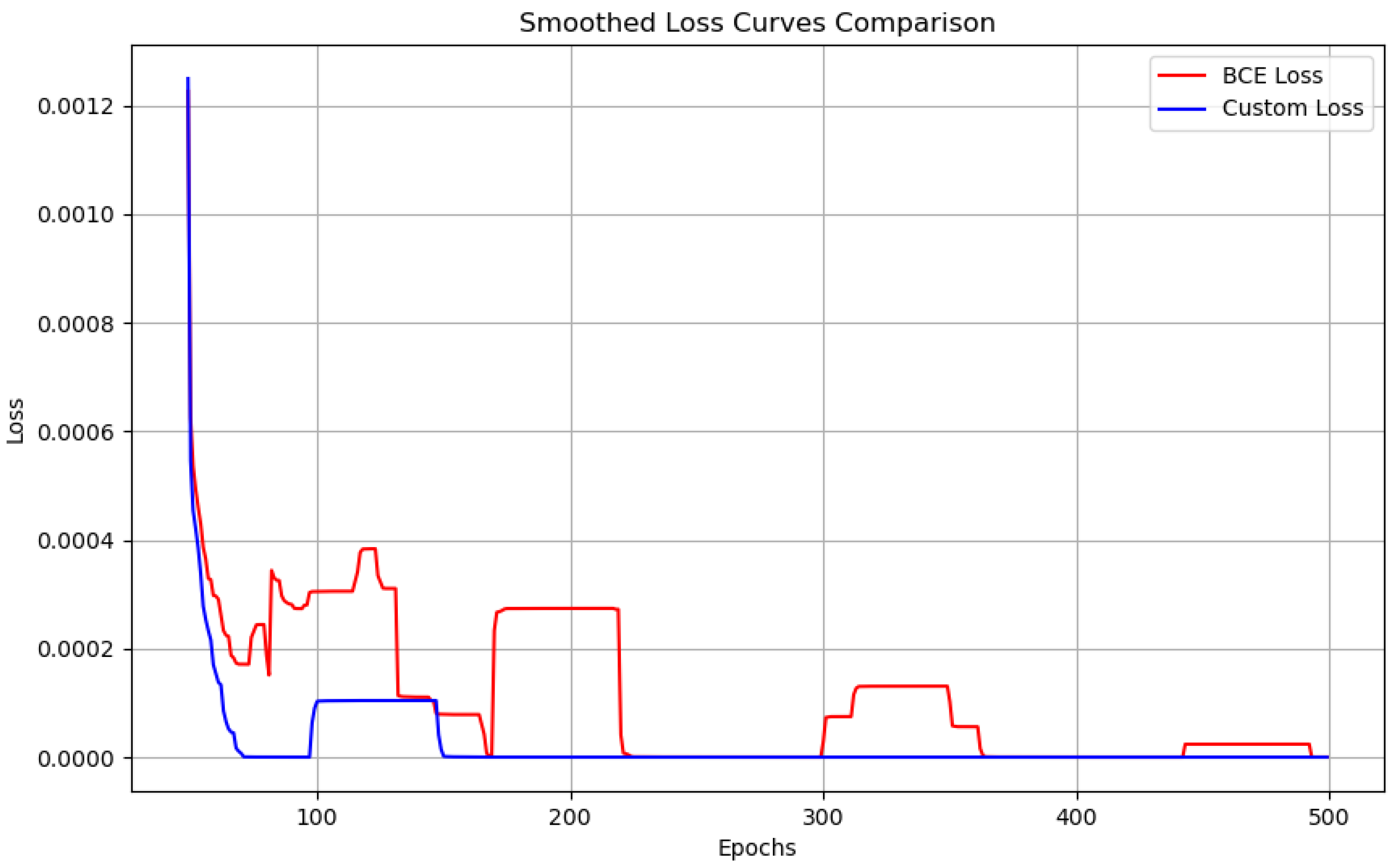
Figure 10.
Comparison of Custom Loss and BCE Loss in logarithmic scale to the y-axis. The Custom Loss exhibits stable convergence, whereas BCE Loss shows oscillatory behavior.
Figure 10.
Comparison of Custom Loss and BCE Loss in logarithmic scale to the y-axis. The Custom Loss exhibits stable convergence, whereas BCE Loss shows oscillatory behavior.
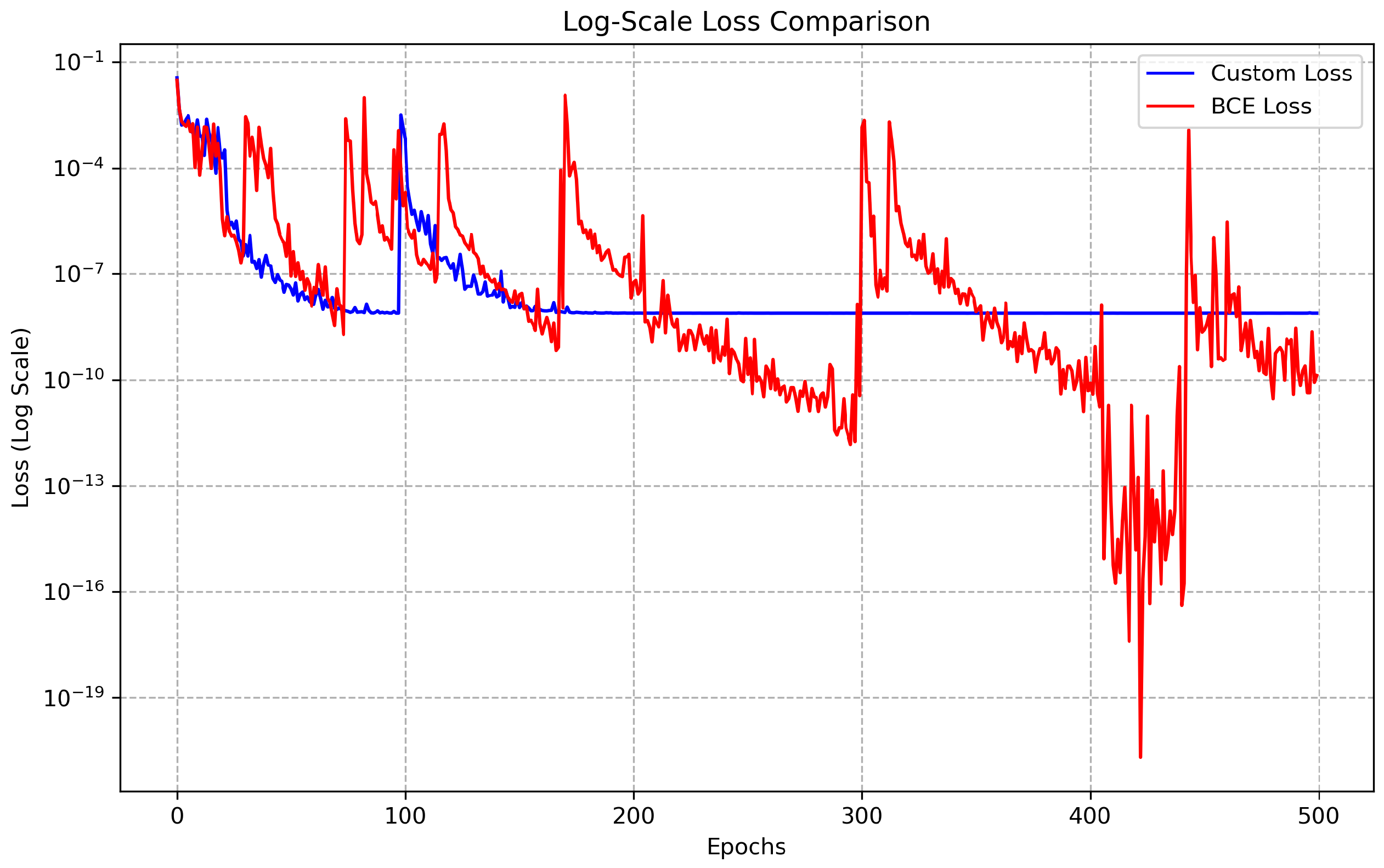
Figure 11.
Histogram and KDE comparison of Custom Loss and BCE Loss distributions. The Custom Loss distribution appears more concentrated with lower variance, whereas BCE Loss exhibits wider spread, indicating greater variability.
Figure 11.
Histogram and KDE comparison of Custom Loss and BCE Loss distributions. The Custom Loss distribution appears more concentrated with lower variance, whereas BCE Loss exhibits wider spread, indicating greater variability.
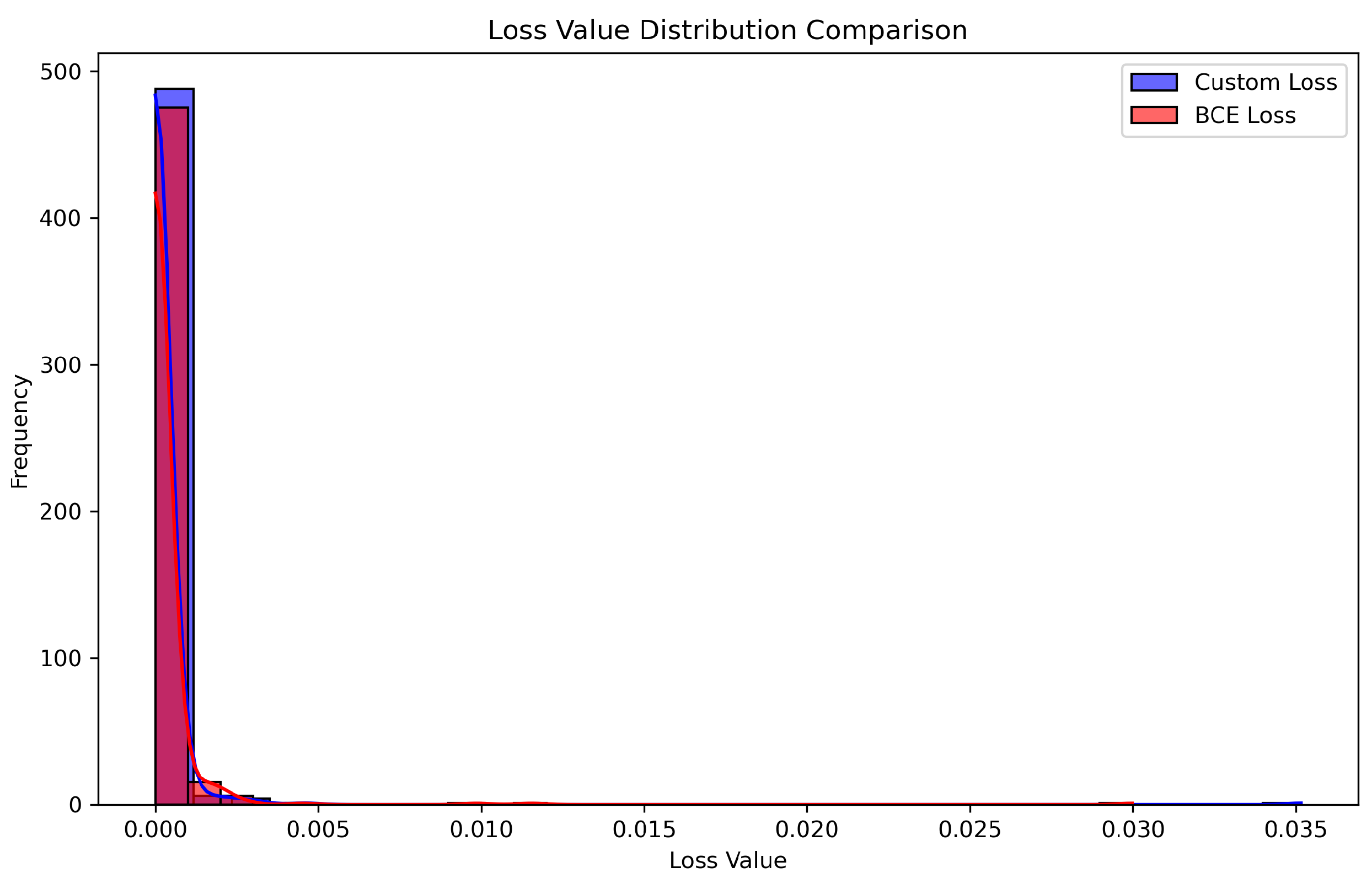
Figure 12.
Log-Scale Loss Plot comparing Custom Loss and BCE Loss. The log transformation reveals stability trends, where Custom Loss exhibits fewer fluctuations and smoother convergence compared to BCE Loss.
Figure 12.
Log-Scale Loss Plot comparing Custom Loss and BCE Loss. The log transformation reveals stability trends, where Custom Loss exhibits fewer fluctuations and smoother convergence compared to BCE Loss.
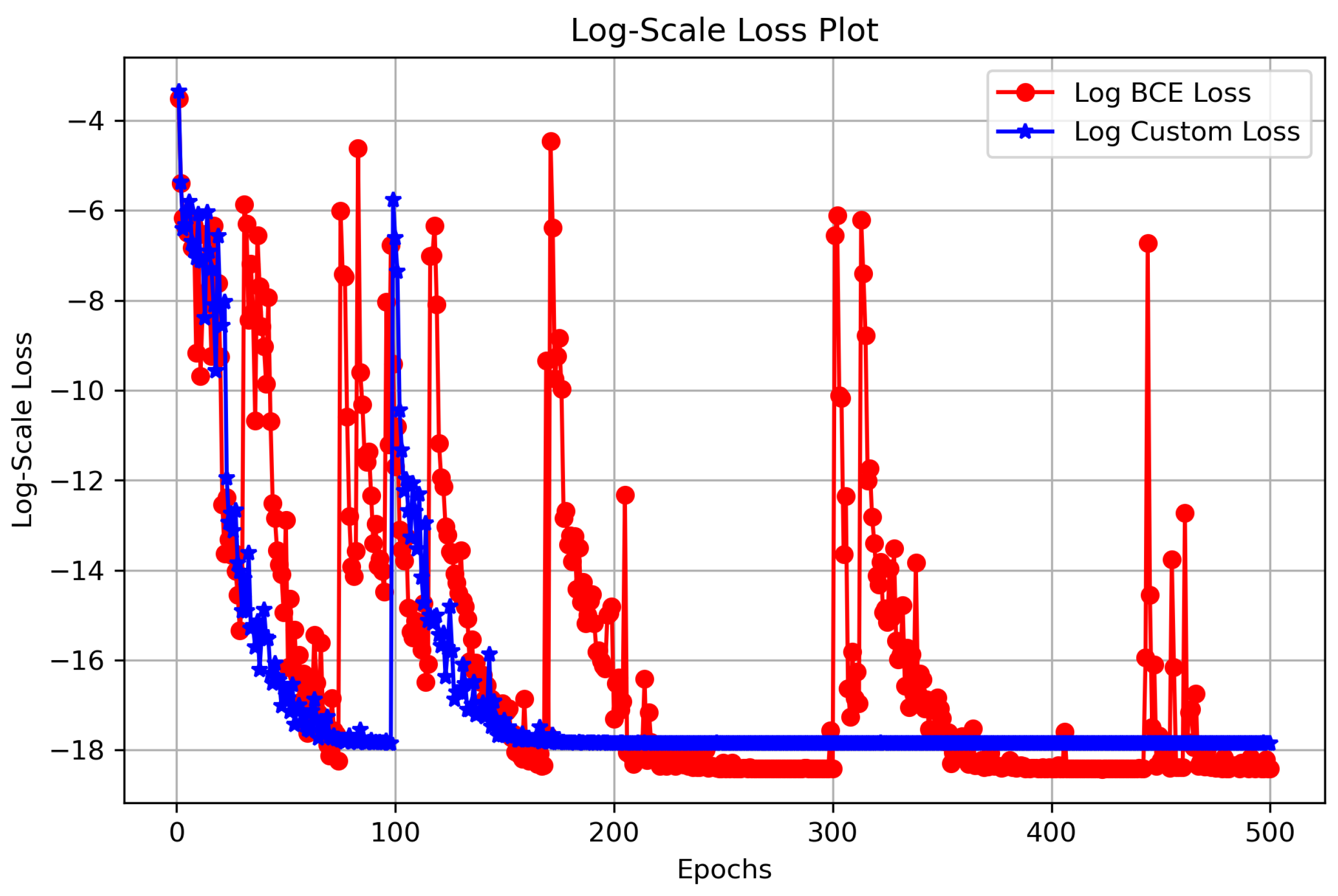
Figure 13.
Epoch-wise Difference (Bar Chart) showing the difference between Custom Loss and BCE Loss at each epoch. A predominantly negative trend suggests that Custom Loss provides lower loss values across training epochs.
Figure 13.
Epoch-wise Difference (Bar Chart) showing the difference between Custom Loss and BCE Loss at each epoch. A predominantly negative trend suggests that Custom Loss provides lower loss values across training epochs.
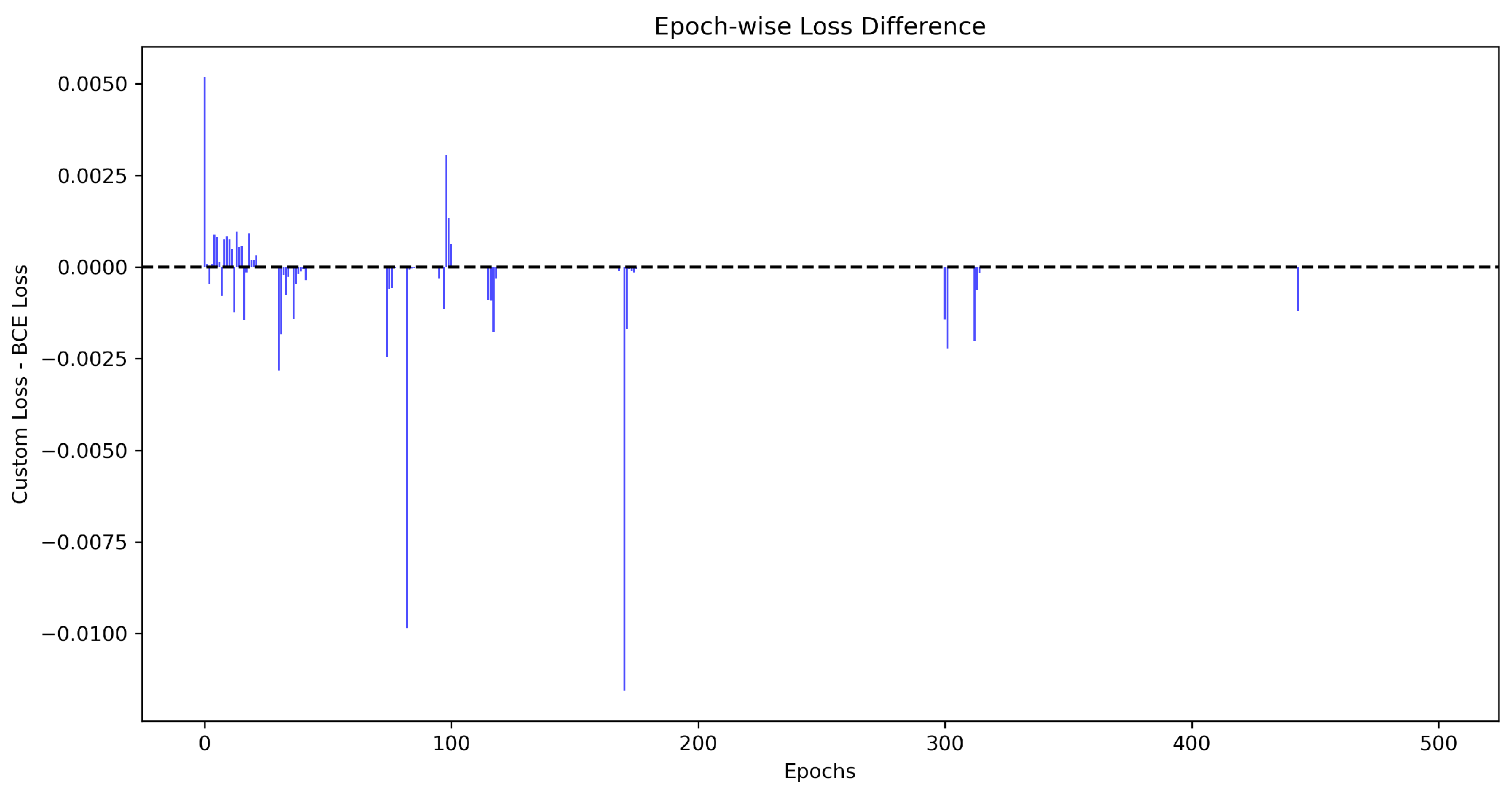
Figure 14.
Scatter Plot with Trend Line illustrating the correlation between BCE Loss and Custom Loss. The fitted trend line indicates a strong positive correlation, confirming that both loss functions exhibit similar behavior, with Custom Loss showing greater stability.
Figure 14.
Scatter Plot with Trend Line illustrating the correlation between BCE Loss and Custom Loss. The fitted trend line indicates a strong positive correlation, confirming that both loss functions exhibit similar behavior, with Custom Loss showing greater stability.
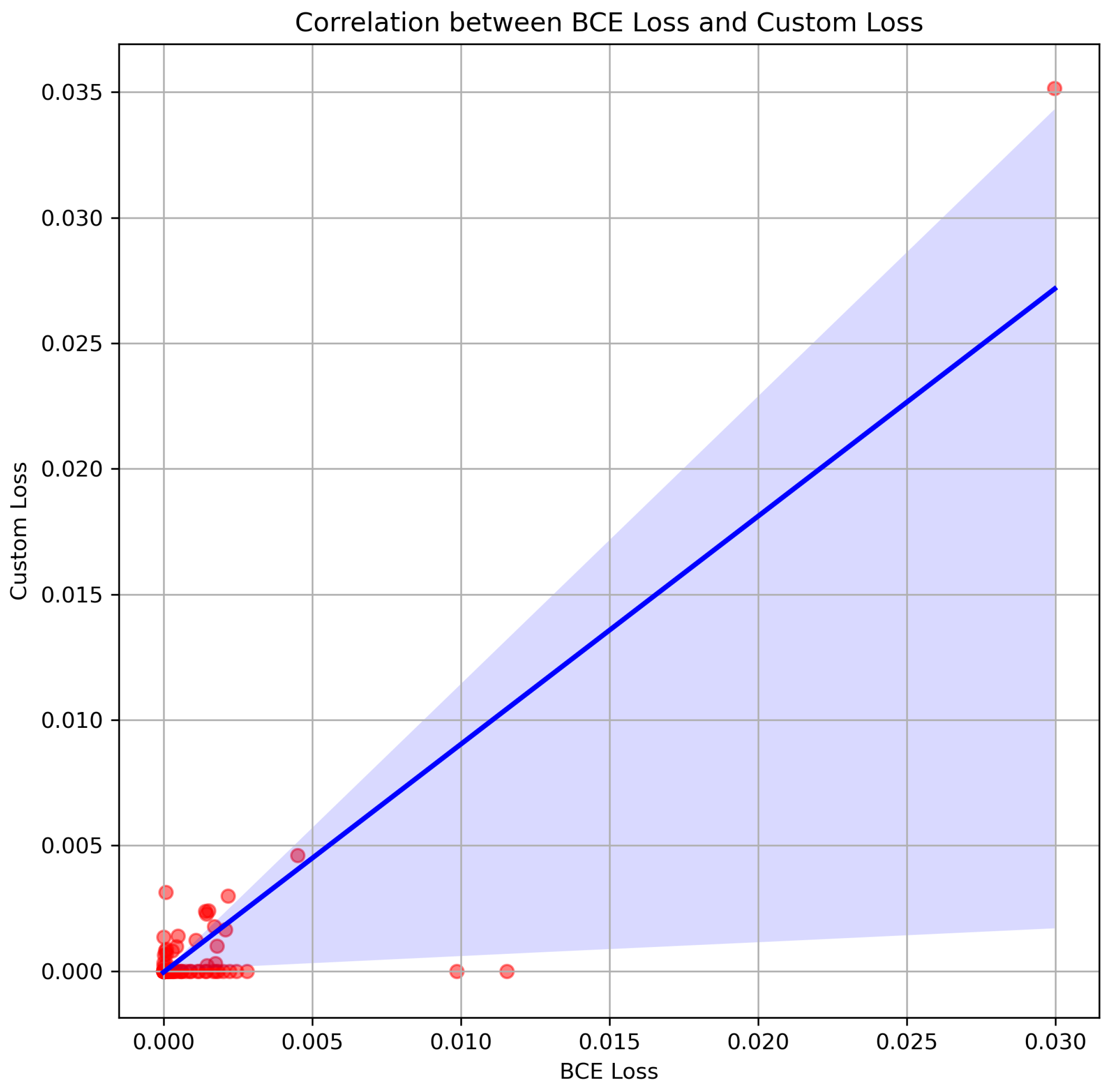
Table 1.
Loss values at selected epochs during training with Custom_Loss.
| Epoch | Loss (Custom_Loss) |
|---|---|
| 5 | 0.002396222773121 |
| 10 | 0.002288330159589 |
| 15 | 0.000985795057823 |
| 40 | 0.000000336587373 |
| 60 | 0.000000014175730 |
| 75 | 0.000000009036549 |
| 100 | 0.001347415337265 |
| 200 | 0.000000007712841 |
| 300 | 0.000000007691881 |
| 450 | 0.000000007710366 |
| 500 | 0.000000007714987 |
Table 2.
Loss values at selected epochs during training with BCE_Loss.
| Epoch | Loss (BCE_Loss) |
|---|---|
| 5 | 0.001510354960826 |
| 10 | 0.001448489814572 |
| 15 | 0.000437349498236 |
| 20 | 0.000095633216917 |
| 25 | 0.000001158516850 |
| 30 | 0.000000457310103 |
| 75 | 0.002460674427018 |
| 100 | 0.000008354524160 |
| 150 | 0.000000014163325 |
| 300 | 0.000000000035069 |
| 450 | 0.000000002202851 |
| 500 | 0.000000000131815 |
Disclaimer/Publisher’s Note: The statements, opinions and data contained in all publications are solely those of the individual author(s) and contributor(s) and not of MDPI and/or the editor(s). MDPI and/or the editor(s) disclaim responsibility for any injury to people or property resulting from any ideas, methods, instructions or products referred to in the content. |
© 2025 by the authors. Licensee MDPI, Basel, Switzerland. This article is an open access article distributed under the terms and conditions of the Creative Commons Attribution (CC BY) license (http://creativecommons.org/licenses/by/4.0/).
Copyright: This open access article is published under a Creative Commons CC BY 4.0 license, which permit the free download, distribution, and reuse, provided that the author and preprint are cited in any reuse.


