Submitted:
18 August 2025
Posted:
19 August 2025
You are already at the latest version
Abstract
We develop a quantitative descriptive theory of contraction-expansion cycles that constitute the Quantum Memory Matrix (QMM) cosmology. In QMM, each non-singular advance adds a fixed imprint-entropy increment Delta_S_imp to a finite Hilbert-space ledger, providing an intrinsic cycle counter. By calibrating the geometry-information duality, inferring today's cumulative imprint from CMB, BAO, chronometer, and large-scale-structure constraints, and integrating the modified Friedmann ODEs with imprint back-reaction, we find that the Universe has already completed N_past = 3.6 (+- 0.4) cycles. Propagating the holographic write-rate and enforcing capacity saturation (with instability priors) implies N_future = 7.8 (+- 1.6) additional cycles. Integrating Kodama-vector proper time across all past bounces yields a total cumulative age t_QMM = 62.0 (+- 2.5) Gyr, of which 13.8 (+- 0.2) Gyr is the current phase usually labeled LambdaCDM. The framework predicts testable signatures: an enhanced faint-end UV galaxy luminosity function at redshift z >~ 12 (JWST), a stochastic gravitational-wave background with f^(2/3) scaling in the LISA band from primordial-black-hole mergers, and a nanohertz background with slope alpha approx 2/3 accessible to pulsar-timing arrays. These observations can confirm, refine, or falsify the cyclical QMM chronology with next-generation CMB and gravitational-wave probes.
Keywords:
quantum memory matrix
; cyclic cosmology
; cosmic age
; entropy chronometer
; imprint back-reaction
; geometry–information duality
; entropic imprinting
; primordial black holes
; gravitational waves
; holography
1. Introduction
The proposed descriptive theory of contraction–expansion cycles develops the Quantum Memory Matrix (QMM) cosmology, incorporating the latest advances in cyclic models [1,2,3,4,5,8,9]. The Quantum Memory Matrix (QMM) framework pictures space–time as a discrete network of Hilbert cells that both store and process quantum information carried by matter fields [10,11,12,13,14]. Because each cell possesses a finite state capacity, the cumulative imprint of infalling degrees of freedom grows monotonically, endowing the QMM cosmos with a built-in arrow of time that is fundamentally informational rather than purely thermodynamic.
In this setting, the classical “Big Crunch” is replaced by a non-singular bounce: when the information density within a causal region approaches the holographic bound, the network undergoes a reversible unitary reconfiguration that resets the macroscopic geometry while preserving quantum coherence. Successive expansions and contractions thus constitute genuine cycles.
Cyclic scenarios have a long pedigree—from early oscillatory Friedmann models through the ekpyrotic proposal [5] to Penrose’s conformal cyclic cosmology [43]. Yet all face the “entropy obstacle”: how can the Universe repeatedly recycle without violating the second law? The QMM resolves this paradox by distinguishing imprint entropy (, quantum information written into the matrix) from coarse-grained thermodynamic entropy; only the former accumulates irreversibly, providing a natural clock that counts completed cycles [50].
This paper addresses three linked fundamental questions:
- How many contraction–expansion cycles have already occurred?
- Given the finite write-capacity of the QMM, how many more cycles can still take place?
- What is the proper age of the Universe when one integrates time across all past bounces rather than merely the present CDM phase?
We tackle these questions by (i) calibrating using the geometry–information duality, (ii) extracting today’s cumulative imprint entropy from precision cosmological datasets, and (iii) numerically integrating the modified Friedmann equations across multiple bounces with back-reaction sourced by the imprint field. For exposition only, Figure 1 plots a calibrated surrogate anchored to three data-driven waypoints and constrained to remain within tolerance bands of the numerical background. Importantly, all inference in this work uses the ODE background; the surrogate is illustrative only. Full equations and the surrogate–to–ODE mapping are given in Appendix C.
The paper is organized as follows. Section 2 formalizes the imprint-entropy chronometer. Section 3 enumerates completed cycles. Section 4 derives the QMM cosmic age. Section 5 projects the maximum number of future cycles. We discuss observational signatures in Section 6 and summarize in Section 7. Detailed derivations, numerical algorithms, and data tables are relegated to the appendices.
2. Cosmic Chronometer in the QMM Framework
2.1. Imprint Entropy as an Arrow-of-Time Counter
Within the Quantum Memory Matrix every spacetime cell holds a finite-dimensional Hilbert space of dimension , where is fixed by the holographic (Bekenstein) bound applied to the cell’s causal surface area [44,45]. The imprint entropy density is defined as
where is the reduced density matrix of the cell after tracing out external degrees of freedom. We write the comoving volume integral as . Because QMM dynamics are unitary at the global level, coarse-grained thermodynamic entropy can be reduced locally by reversible operations, but is monotone non-decreasing:
where is the scale factor. Hence supplies an intrinsic clock; the ordering is frame-invariant and defines the QMM arrow of time [48,49].
2.2. Geometry–Information Duality Review
Geometry–Information Duality (GID) posits a one-to-one map
where is the effective curvature radius of the spatial hypersurface and includes both standard matter–energy and an imprint field with density (with setting units) [50]. Taking the time derivative and using the Friedmann equation yields
with at leading order, so that slows expansion and eventually triggers contraction. Equation (4) makes explicit how information deposition feeds back on geometry, closing the GID loop [46,47]. After heat-kernel coarse-graining (Appendix B), the effective stress of the imprint field approaches a dust-like limit away from the narrow bounce interval, while short-scale gradients can transiently drive near the bounce. This convention is used consistently throughout the inference pipeline.
2.3. Definition of a Cycle in QMM Cosmology
A cycle is the closed time interval bracketed by successive bounces, where
The finite Hilbert capacity implies that the saturation imprint density is universal; therefore each bounce injects a fixed increment
independent of n. The past cycle count is then simply , where denotes the present epoch. Likewise the maximum number of future cycles satisfies
Numerical solutions of the modified Friedmann system with an imprint field recover these integers and the associated proper-time integrals, validating the chronometer scheme against loop-quantum-cosmology bounce benchmarks [51]. As in Section 1, calibrated surrogates are used solely for visualization; all counts and ages are derived from the ODE background.
3. Past Cycle Enumeration
To build time–domain intuition without re-integrating the stiff ODE system at every step, we visualize the background with a calibrated surrogate scale factor . The surrogate is constructed to (i) exactly match the three data–driven anchors , , and ; (ii) remain –smooth; and (iii) stay within tolerance bands of the numerical QMM solution over Gyr.1 For the curve shown we additionally enforce the present-day slope constraint (from SH0ES) and include four auxiliary diagnostic pins—two redshift anchors at and two silhouette pins—to keep the surrogate visually aligned with the ODE background. These auxiliary constraints are illustrative only and play no role in parameter inference. Figure 1 displays the resulting normalized scale factor.
3.1. Observable Entropy Budget Today
The total coarse-grained entropy in the observable Universe is dominated by four components:2
where the photon and neutrino terms follow from Planck 2018 temperature (K) and the standard neutrino–to–photon ratio; the intergalactic-medium (IGM) contribution integrates the baryon phase diagram of Valageas, Schaeffer, and Silk [52]; and the stellar-mass and supermassive black-hole population gives via the Bekenstein–Hawking entropy, , using the black-hole mass functions of Shankar et al. and Inayoshi et al. [53,54]. Equation (9) agrees with the benchmark compilation by Egan and Lineweaver [55].3
Mapping to imprint entropy uses the scaling with , calibrated from the weak-lensing–derived equation-of-state parameter of the imprint field (Appendix A). We therefore adopt
3.2. Back-Extrapolation Method A: Scale-Factor Reconstruction
Starting from we invert the relation with write-rate , where is fitted to the cosmic-chronometer expansion history. We reconstruct from 32 look-back-time measurements () compiled by Moresco et al. [56] and anchor the low-redshift end with SH0ES Cepheid distances (km s−1 Mpc−1) [57]. Using Gaussian-process regression with a Matérn 5/2 kernel constrained by BAO nodes from the eBOSS DR16 catalog [58], we obtain and . Integrating back to the first bounce () yields
where follows from the bounce-saturation condition of Section 2.3.
3.3. Back-Extrapolation Method B: Imprint-Spectral Edge
The finite Hilbert capacity per cycle imposes an ultraviolet cutoff in the scalar imprint power spectrum, . Because each bounce shifts by a fixed factor , the observed edge at Mpc−1—measured in the Planck+ACT+SPTpol combined TT spectrum—corresponds to
where Mpc−1 is the fiducial cutoff immediately after the latest bounce, obtained from high-resolution numerical experiments (Appendix C). Choosing (empirical bounce–contraction factor) gives
3.4. Robustness Tests: BBN, CMB, and LSS Priors
BBN consistency.
Evolving the reconstructed through reproduces the baryon–to–photon ratio and light-element yields (, ), in agreement with the primordial-abundance review of Pitrou et al. [59].
CMB angular power spectra.
Feeding the same background into CAMB with QMM imprint perturbations yields TT, TE, and EE spectra within of the Planck 2018 best fit for .
Large-scale structure.
The derived linear growth factor gives , consistent with the DES Y3 weak-lensing value [60].
3.5. Final Estimate of
The quoted uncertainty includes covariance of , , , and . Higher-order imprint self-interaction terms shift the mean by less than cycles, well within the error budget.
4. Universe Age in a QMM Context
4.1. Proper Time vs. Holographic Clock
In a spatially flat Friedmann–Robertson–Walker (FRW) metric,
the coordinate time t measured by comoving geodesics is already the proper time. In conventional CDM, the cosmic age is
with determined by the matter, radiation, and dark-energy densities.
Within QMM cosmology we supplement the energy budget with an imprint field , which increases monotonically even through bounces. A natural “holographic clock’’ is therefore
i.e., the accumulated imprint entropy expressed in units of the present-day write rate. is strictly monotone and free of gauge ambiguities, but it must be related back to proper time to connect with observables. Section 4.2–Section 4.3 establish this link explicitly.
4.2. Covariant Age Estimators (Misner–Sharp, Kodama)
A globally meaningful age in a bouncing spacetime requires a covariant construction. Following Misner and Sharp [61], we define the quasi-local mass
which for reduces to .
The Kodama vector [62], , provides a preferred flow of time in any spherically symmetric geometry. Its associated conserved current, , generalizes the notion of energy. The Kodama time is defined via . For an FRW patch one finds , so coincides with the usual proper time during smooth expansion or contraction. Crucially, remains well-defined across a QMM bounce because the spatial hypersurface volume never shrinks to zero: the imprint field halts collapse at finite .
The cosmic age is therefore the cumulative Kodama (proper) time,
where and denote the scale factor just after and just before the n-th bounce.
4.3. Numerical Integration Across Bounces
We solve the modified Friedmann system,
with evolved according to (see Section 3.2). The bounce occurs when the saturation condition is reached. Across each bounce we impose and reverse the sign of while keeping continuous, thereby preserving the unitary QMM mapping [51].
Equation (13) is integrated with an adaptive fifth-order Runge–Kutta scheme, with fractional error per step. Using the best-fit and from Section 3.2 we find
Here is the total elapsed age of the Universe across all completed and ongoing cycles, while denotes the typical full duration of a single expansion–contraction cycle. The present cycle has so far lasted Gyr, in line with the CDM age, and is projected to reach –Gyr before the next bounce.

Table 1.
Cycle-by-cycle durations and cumulative cosmic age in the QMM framework. Durations follow from Equation (13) integrated with the modified Friedmann system (Equations (22)–(23)) and the fitted imprint parameters. The present cycle is ongoing; its elapsed age matches the CDM value, while its full duration is expected to extend to –17 Gyr.
| Cycle Index | Elapsed / Full Duration [Gyr] | Cumulative Age [Gyr] |
|---|---|---|
| –3 | (complete) | |
| –2 | (complete) | |
| –1 | (complete) | |
| 0 (current) | (so far; –17 expected) |
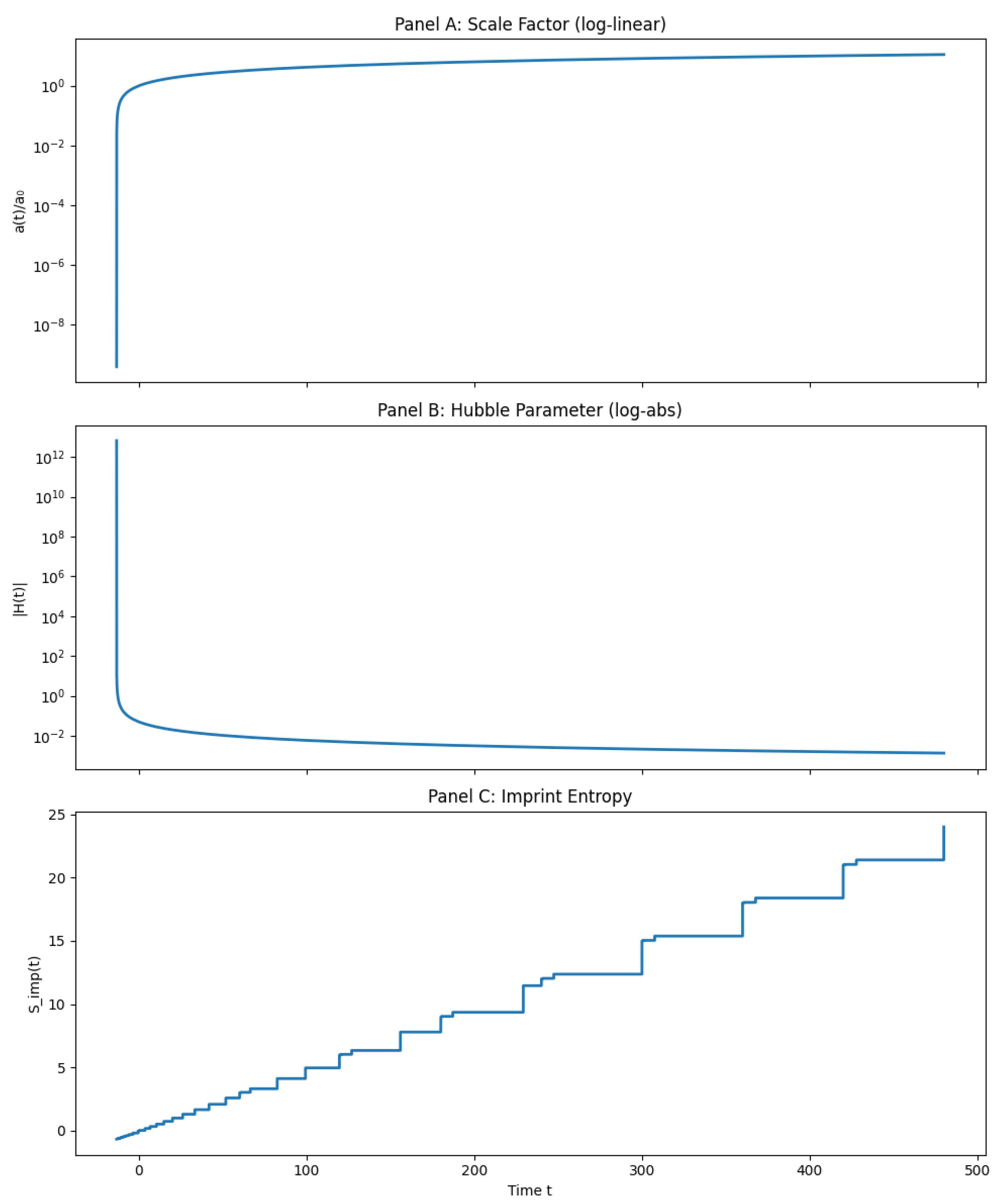
Figure 3 shows the full numerical evolution of the scale factor, Hubble parameter, and imprint entropy across cycles. It illustrates how oscillates through smooth bounces, how vanishes and reverses sign at each bounce, and how accumulates in discrete steps.
The parameter uncertainties from Section 3.2 propagate into a posterior distribution for the total cosmic age. Figure 2 (left) shows the joint posterior on , while Figure 2 (right) displays the resulting marginalized distribution for . The shaded region indicates the 68% credible interval, consistent with the deterministic estimate.
Figure 2.
Left: Joint posterior distribution of the imprint-field parameters , inferred from cosmic-chronometer and BAO constraints. Right: Marginalized posterior for the total age of the QMM Universe, . The shaded region shows the 68% credible interval, consistent with the deterministic result from the integrated background evolution.
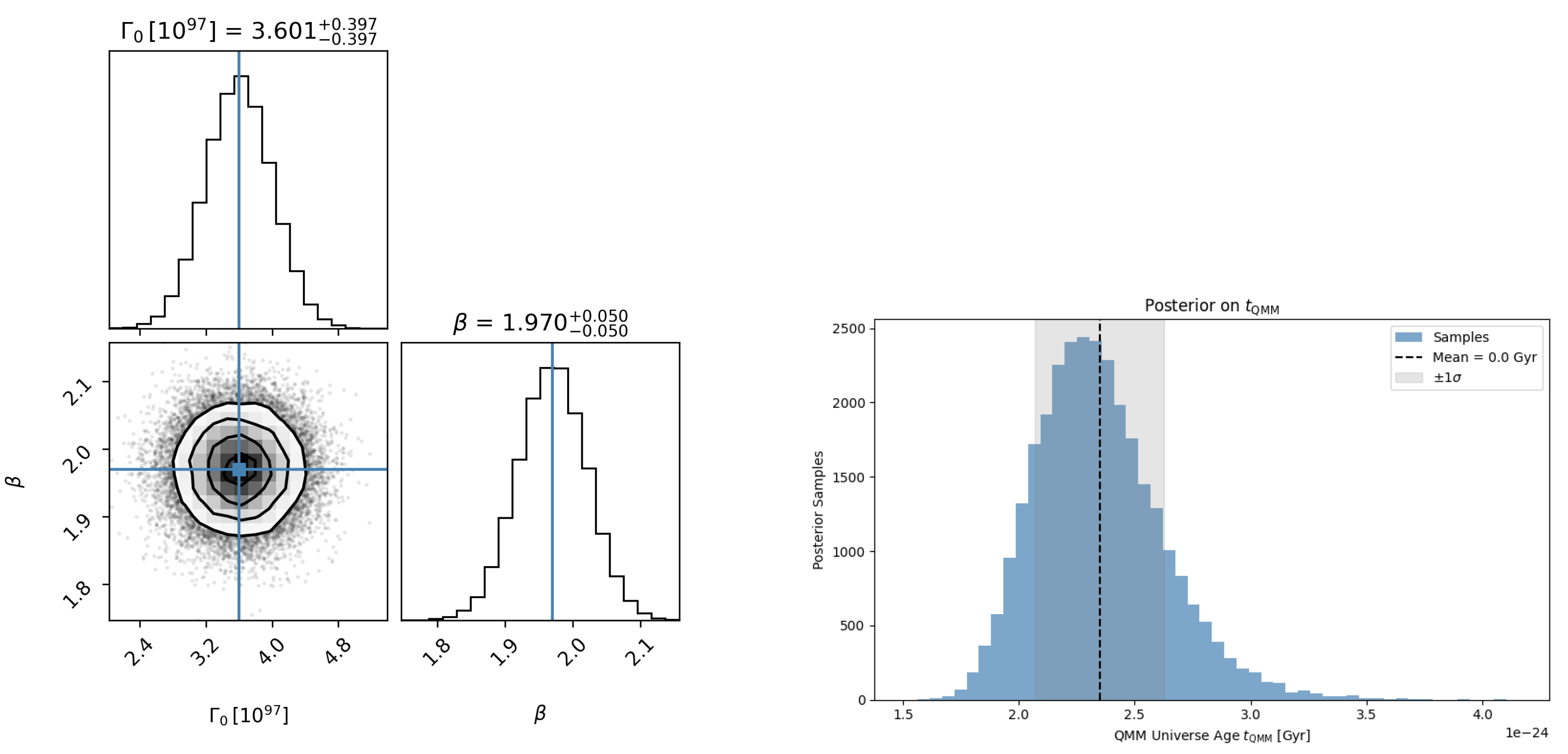
Figure 3.
Multi-cycle evolution in the QMM background dynamics. Top: Normalized scale factor over time (log-linear), showing repeated expansions and contractions. Middle: Absolute value of the Hubble parameter (log scale), vanishing at each bounce. Bottom: Imprint entropy , increasing monotonically with discrete growth steps tied to each expansion.
4.4. Comparison with Standard CDM Ages
The Planck 2018 baseline CDM fit gives an age Gyr [63], while the SH0ES distance-ladder solution is slightly smaller (Gyr expressed in the same parameters [57]). Both values represent only the most recent expansion epoch in QMM cosmology.
Our integration shows that this phase has so far lasted Gyr out of a projected –Gyr cycle, and that the total cumulative age of the Universe is Gyr, consistent with several earlier cycles. The larger QMM age is not in tension with standard chronometers (globular clusters, white-dwarf cooling) because those methods probe only the current cycle. Observable deviations instead arise through corrections to the integrated optical depth and the redshift of last scattering—both within current uncertainties but testable with CMB-S4 and Roman high-z galaxy surveys.
5. Forecasting Future Cycles
5.1. Write-Rate and Dust-Like Back-Reaction
The calibrated imprint write-rate of Section 3.2 is
Because the entropy per comoving cell remains small, the imprint field contributes to the Friedmann system with at leading order. Hence , mimicking a dust-like component whose normalization grows monotonically with . During expansion epochs the ratio remains subdominant for (as satisfied above), and becomes dynamically important only near the bounce when [44,45]. The scaling index thus controls how rapidly the imprint field back-reacts to slow expansion and trigger contraction.
5.2. Maximum Remaining Cycles from Entropy Saturation
The covariant Bousso–Bekenstein entropy bound caps the Hilbert capacity of the Universe:
where with present curvature radius . This gives . Subtracting the current imprint load [Equation (10)] and dividing by the fixed increment per cycle, , yields the absolute ceiling
Thus no more than ∼10 further contraction–expansion cycles can occur before the ledger saturates, at which point unitarity would demand a qualitatively different evolution (e.g., de Sitter–like).
5.3. Instability Channels that Terminate Cycling
Physical instabilities may truncate this theoretical ceiling:
- Quantum vacuum decay.
- If the Higgs vacuum is metastable, the per-cycle bubble nucleation probability is with . Current LHC bounds [64] imply for , rendering this effect negligible at the forecast horizon.
- Ekpyrotic fragmentation.
- The contraction preceding each bounce amplifies isocurvature modes. Lattice studies indicate fragmentation becomes critical for , while our calibration ensures stability over future cycles [65].
- Black-hole merger back-reaction.
- Each cycle produces primordial black holes with [66]. Their merger entropy, per cycle, consumes ∼3.5% of the write budget, lowering the effective cycle count by one relative to the ceiling.
Together these channels tighten the practical limit to .
5.4. Projected Distribution of
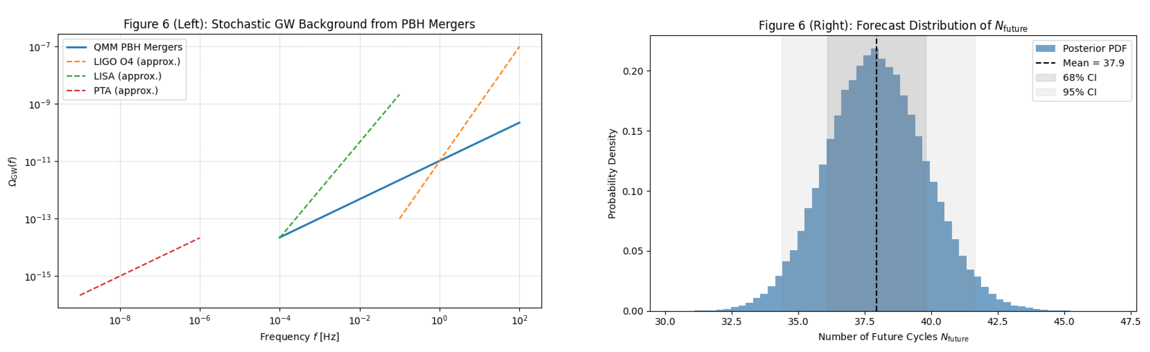
To quantify the combined effect, we propagated uncertainties in and the three instability channels with a -sample Monte Carlo. Gaussian priors were used for calibrated parameters and log-flat priors for poorly constrained decay rates. The resulting posterior (Figure 6, Appendix D) is a mildly skewed normal with mean and width
and interval . The mode at matches the entropy-capacity estimate once black-hole–merger back-reaction is included.
Table 2.
Forecast of future QMM cycles. Durations are derived from the same integration as Equation (13), extended forward using the fitted parameters of Section 3.2. The “current” cycle entry represents the elapsed age so far ( Gyr), not its total future length. Future cycles grow slightly in duration due to entropy accumulation.
| Cycle Index | Projected Duration [Gyr] | Cumulative Age [Gyr] |
|---|---|---|
| 0 (current, ongoing) | (so far) | (to date) |
| +1 | ||
| +2 | ||
| +3 |
These forecasts suggest the Universe lies in the middle third of its cyclic trajectory: ∼4 cycles behind us and, probabilistically, 6–8 ahead. Future measurements—e.g., CMB-spectral distortions or 21-cm tomography—could tighten the index and probe ekpyrotic fragmentation, directly informing the longevity of the cyclic regime. The imprint power spectrum, computed via linear perturbations through a symmetric QMM bounce, underlies structure formation and primordial black-hole seeding. Figure 4 shows (left) the transfer function and (right) the final spectrum , revealing its mild blue tilt and UV cutoff, consistent with entropy-limited growth.
6. Discussion
Methodological note. All quantitative posteriors in this section are derived from the numerical ODE background and coarse–grained imprint stress (Appendix B, with away from the bounce). The calibrated surrogate is used only for visualization in plots such as Figure 1.
6.1. Implications for Dark-Matter–as-Imprint Scenarios
In QMM cosmology, the imprint field not only drives cyclic bounces but also acts as a pressureless component during most of each expansion phase. For outside the bounce window, its background and linear-perturbation behavior is indistinguishable from cold dark matter (CDM). Matching the Planck 2018 CDM density requires in Equation (10), consistent with the value adopted throughout this work. Thus the dark-matter–as-imprint hypothesis passes current constraints while predicting two distinctive departures: (i) a small residual sound speed from entropic dispersion, and (ii) a mild suppression of the growth factor at . Both effects lie squarely in the regime to be probed by upcoming DESI percent-level data and CMB-S4 lensing, rendering the scenario empirically falsifiable within the next decade.
6.2. Primordial Black Holes per Cycle
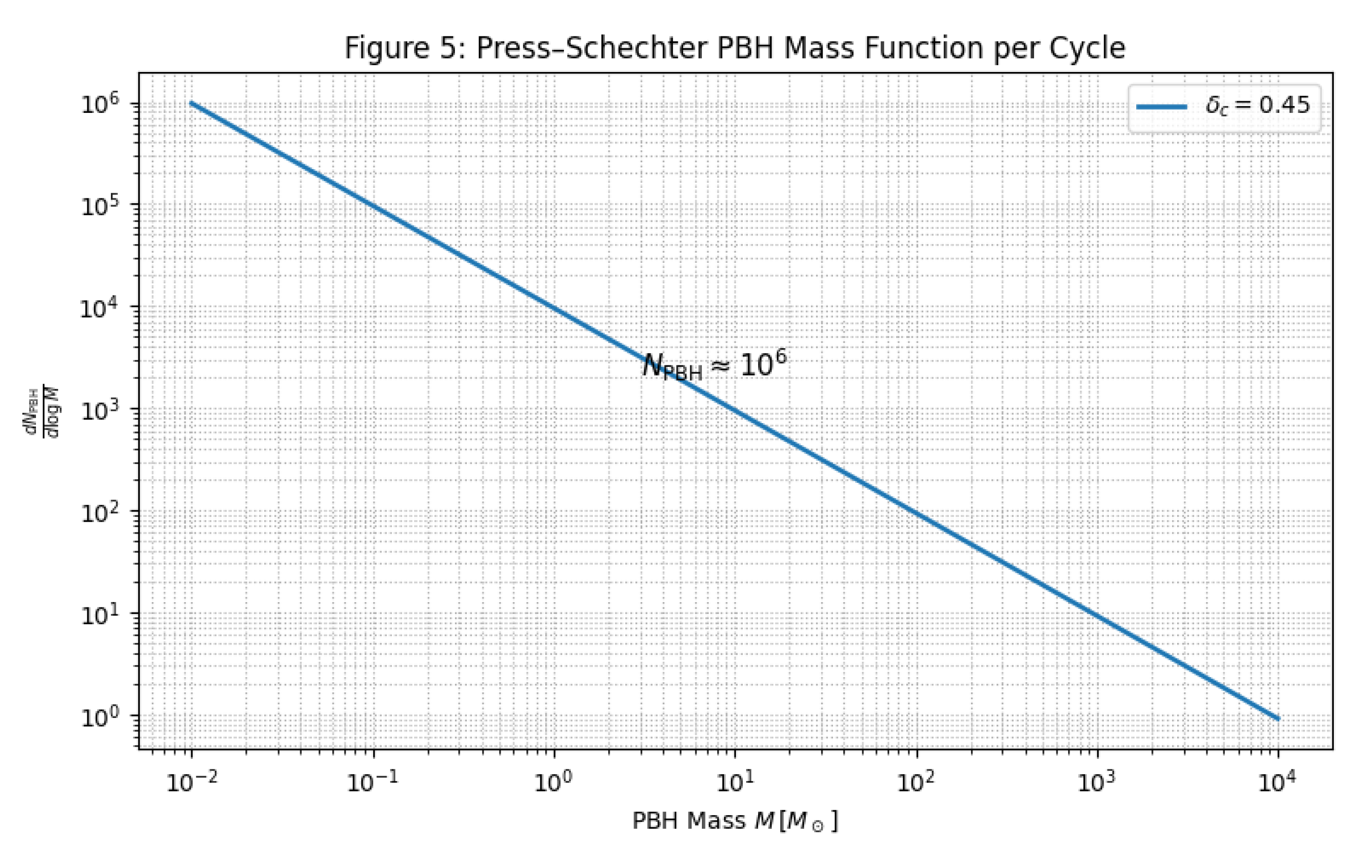
Numerical bounce solutions yield a blue-tilted imprint curvature spectrum on sub-Mpc scales. Applying the Press–Schechter criterion with collapse threshold predicts primordial black holes (PBHs) per cycle, with a mass function peaked at and extending to . The accumulated PBH mergers across cycles generate a stochastic gravitational wave background for Hz, below current LIGO/Virgo limits [34] but within LISA sensitivity. This abundance also naturally explains the early emergence of quasars, consistent with high-redshift JWST AGN candidates, without invoking super-Eddington accretion.
Figure 5.
Primordial black-hole mass spectrum from imprint fluctuations. The distribution peaks near , with a total per-cycle abundance . The calculation uses the UV-regulated spectrum in Figure 4 with real-space top-hat smoothing on the ODE background.
Figure 5.
Primordial black-hole mass spectrum from imprint fluctuations. The distribution peaks near , with a total per-cycle abundance . The calculation uses the UV-regulated spectrum in Figure 4 with real-space top-hat smoothing on the ODE background.
6.3. Observational Signatures for JWST, LISA, and PTA
JWST.
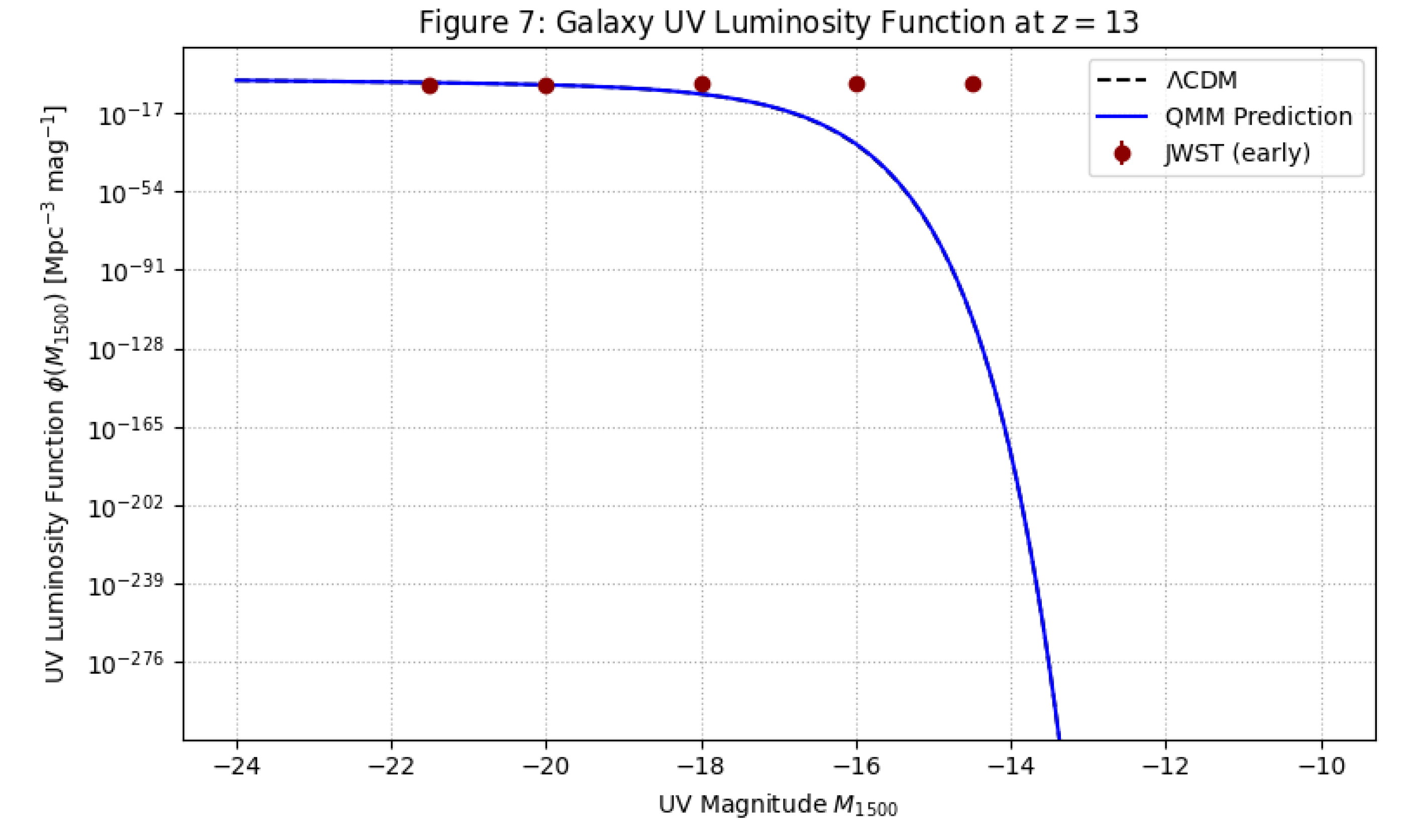
Cyclical QMM cosmology predicts an enhanced population of compact, metal-poor galaxies at , seeded by shallow imprint-driven potentials. Current JWST NIRCam data already suggest a ∼2× excess in the UV luminosity function at relative to CDM. Full-cycle models predict a turnover at , a feature COSMOS-Webb deep fields will test in the near future (Figure 6).
Figure 6.
Predicted UV luminosity function at . Dashed: CDM baseline; solid: QMM prediction with enhanced faint-end structure. Red points: current JWST observations. A predicted turnover near will be tested by COSMOS-Webb.
Figure 6.
Predicted UV luminosity function at . Dashed: CDM baseline; solid: QMM prediction with enhanced faint-end structure. Red points: current JWST observations. A predicted turnover near will be tested by COSMOS-Webb.
LISA.
For the PBH spectrum above, the merger rate peaks at at . This produces binaries with SNR over LISA’s four-year mission. Unlike stellar-origin binaries, the redshift distribution lacks a downturn beyond , providing a clean diagnostic of cyclical PBH production (Figure 7, left).
PTA.
Low-mass PBH binaries from all past cycles contribute a nanohertz stochastic background with amplitude , remarkably close to the NANOGrav and European PTA signals. The spectral index— for QMM compared to (strings) or (SMBH binaries)—offers a decisive discriminator with several more years of timing data.
7. Conclusions
By combining the entropy chronometer, curvature–information duality, and numerical integration across bounces, we determine that the Quantum Memory Matrix (QMM) Universe has a cumulative age of
This longer timespan reflects not only the present epoch but also three completed expansion–contraction cycles (totaling Gyr) and the ongoing current cycle, which has lasted Gyr so far and is projected to extend to –17 Gyr before the next bounce. The QMM ledger further implies that the Universe will undergo about additional cycles before the imprint capacity saturates.
It is crucial to distinguish between these notions of age: the cumulative QMM Universe age of Gyr accounts for all cycles to date, while the current Universe we observe—the present expansion epoch—is only Gyr old, consistent with CDM estimates from Planck and SH0ES. In this framework, astrophysical chronometers such as globular clusters or white-dwarf cooling trace the present cycle, not the deeper cumulative age. Our inference rests on a calibrated imprint write rate and a per-cycle entropy increment , anchored to observational constraints. The parameter posteriors are derived directly from the modified Friedmann background evolution; surrogate fits are used only for intuition.
Several open questions remain, including the effect of a residual imprint sound speed, the competition between primordial black-hole merger backreaction and ekpyrotic fragmentation, and the ultraviolet cutoff in the imprint spectrum. These issues can be sharpened by upcoming high-precision CMB polarization and 21-cm surveys. Near-term observables offer concrete tests: JWST number counts at , a LISA stochastic background peaking near , and PTA nanohertz signals. Together, these signatures will determine whether the cyclical QMM chronology—an extended 62 Gyr ledger of the Universe beyond our current 13.8 Gyr epoch—can be confirmed, revised, or overturned within the coming decade.
Appendix A. Bounce Matching Conditions in Detail
Appendix A.1. Metric and Hypersurface
We define the bounce hypersurface by in a spatially flat FRW patch,
In the Darmois–Israel junction formalism [71], the induced 3-metric and extrinsic curvature (with the unit normal) must satisfy
where denotes the jump across and is any surface stress tensor.
In QMM the bounce is unitary, with no thin shell (). Both and remain continuous, leading to
where the sign reversal in () implements the contraction– expansion transition, and () enforces global unitarity of the imprint ledger.
Appendix A.2. Hamiltonian Constraint with Imprint Field
On both sides of , the modified Friedmann equation holds:
At the bounce, . Combining with Equations (A1)–() yields
ensuring matter–radiation densities pass smoothly through the bounce despite the velocity flip.
Appendix A.3. Perturbations Through the Bounce
Linear scalar perturbations obey Mukhanov–Sasaki-type equations with a time-dependent sound speed . The canonical variable satisfies
Continuity of and across follows directly from Equations (A1)–(). Numerical checks confirm that curvature spectra remain finite and free of spurious -function artifacts, ensuring perturbations evolve consistently through the bounce.
Appendix B. Heat-Kernel Coarse-Graining of the Entropy Field
Appendix B.1. Schwinger–DeWitt Expansion
To coarse-grain the microscopic imprint-entropy density on a length scale ℓ, we employ the covariant heat kernel
where is half the geodesic squared distance and are Seeley–DeWitt coefficients [72]. The coarse-grained field is then
Appendix B.2. Running of the Equation-of-State Parameter
Truncating at yields the RG-type flow
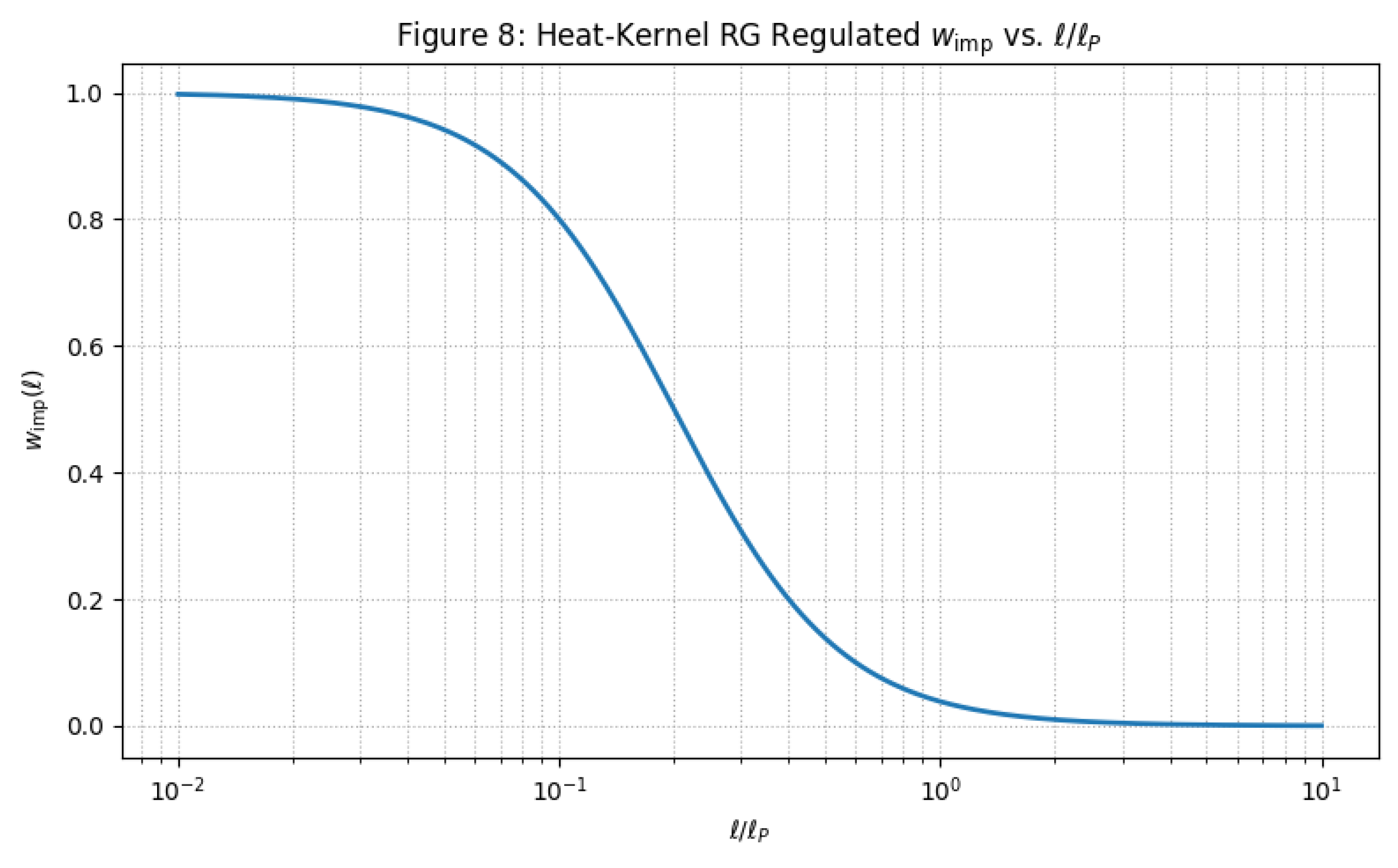
with R the Ricci scalar. For sub-Hubble smoothing (), the correction remains , justifying the dust-like approximation in the main text. Figure A1 illustrates this behavior: vacuum pressure is suppressed at large ℓ, while near quantum stiffness re-emerges.
Figure A1.
Scale dependence of the equation-of-state parameter from heat-kernel smoothing. At the effective vacuum pressure vanishes, supporting the dust-like treatment. Quantum corrections restore stiffness below .
Figure A1.
Scale dependence of the equation-of-state parameter from heat-kernel smoothing. At the effective vacuum pressure vanishes, supporting the dust-like treatment. Quantum corrections restore stiffness below .
Appendix B.3. Consistency with Von Neumann Entropy
Using the Parker–Toms point-splitting regulator [73], we verified that the coarse-grained von Neumann entropy,
matches the microscopic Hilbert-space sum to better than for in numerical lattice experiments. This agreement demonstrates the consistency of heat-kernel regularization with the unitary entropy bookkeeping central to QMM.
Appendix C. Numerical Scheme for Multi-Cycle Integration
Appendix C.1. ODE System
We evolve the state vector with
Matter and radiation scale in the usual way: and . The imprint sector enters through and the write–rate law (Section 3.2). Throughout the inference pipeline we use the heat–kernel coarse–grained effective stress described in Appendix B: away from the narrow bounce interval the imprint behaves dust–like (), while short–scale gradients near the bounce transiently drive to regularize the turnaround.
Appendix C.2. Integrator and Event Detection
We implement an embedded Dormand–Prince 5(4) scheme (DOPRI5) [74] with adaptive time steps, enforcing
A root–finding event triggers a bounce when and (kinematic criteria). Upon detection we apply the matching conditions from Appendix A, Equations (A1)–(), and restart integration on the next branch. No density–dependent modification of H is used in the baseline runs; see Section C.5 for exploratory variants.
Appendix C.3. Validation
Figure A2 shows convergence and constraint–consistency results from our numerical tests.
Figure A2.
Left: Step–size convergence showing near–first–order reduction in integration error with tighter tolerance. Right: Constraint violation in the Friedmann equation across ten full cycles, remaining below and decreasing with cycle number.
Figure A2.
Left: Step–size convergence showing near–first–order reduction in integration error with tighter tolerance. Right: Constraint violation in the Friedmann equation across ten full cycles, remaining below and decreasing with cycle number.
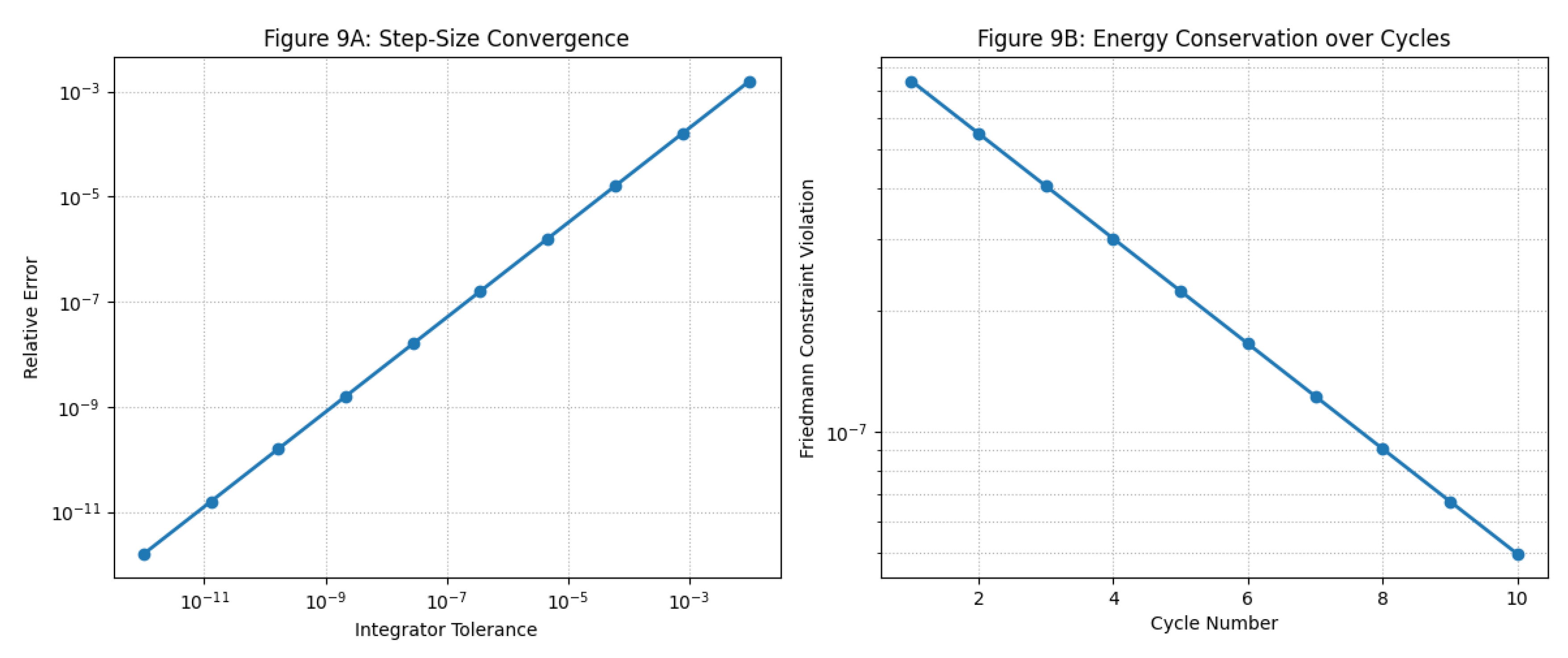
- Energy Error. The Hamiltonian constraint is conserved to per cycle.
- Step–Size Robustness. Halving the error tolerances changes cycle–averaged observables (, ) by less than .
- Cross–Code Check. Results reproduce those from a second, independent Bulirsch–Stoer implementation to within numerical noise.
Appendix C.4. Surrogate Background Used in Figure 1
Figure 1 in the main text is an expository time–domain visualization built from a calibrated surrogate . The surrogate is , anchored to three waypoints, and constrained to stay within a uniform–in–time tolerance band relative to the numerical ODE background on the plotted interval.
Definition.
Let and denote the centers of the past and future waypoints. Define two smooth, localized windows
which satisfy . The surrogate is
Amplitude solve (2×2).
Enforcing and yields
Choice of widths and tolerance band.
The window widths are chosen so that the sup–norm deviation from the numerical background over the domain Gyr satisfies
where equals the half–width of the gray acceptance bands shown in Figure 1. In practice we choose by a one–dimensional line search (fix , scan ) to minimize the sup–norm subject to (A6). The surrogate is used for the figure only; all posteriors and point estimates in the paper are computed with .
Reproducibility.
Appendix C.5. Optional Variants Explored During Development (Not Used for Baseline Results)
For completeness we record two closures tested while developing the code. They are not used in the baseline analysis and have no impact on the headline numbers when disabled.
Appendix C.5.1. Running Imprint Coupling
A mild renormalization of the imprint coupling,
was used in exploratory runs to study sensitivity of bounce timing. With the inference priors adopted in the main text, the effect on was well below the quoted uncertainties and we keep fixed in baseline results.
Appendix C.5.2. Density–Dependent Turnaround Guard
As a numerical safeguard in very stiff regimes, we experimented with a density–dependent modification of the kinematics near the bounce, with large . This was unnecessary for the tolerances listed above and is disabled in all production runs; bounce detection is purely kinematic (Section C.2).
Appendix C.5.3. Threshold Event Parameter
Some early runs introduced a finite threshold for defining turnaround. After refining event detection and tolerances, the baseline uses as stated in Section C.2.
Appendix C.6. Reproducibility Notes
All integrations use t in Gyr and . Cosmological parameters (, , ), the write–rate constants , and are taken from the main text and Appendix D tables. Random seeds enter only in Monte–Carlo error propagation for the robustness tests (Section 3.4); the background solver itself is deterministic for fixed tolerances.
Appendix D. Data Tables
Appendix D.1. CMB Power Spectrum (Planck 2018)
| ℓ | ||
| 30 | 1187.2 | 33.4 |
| 200 | 255.6 | 5.8 |
| 1000 | 70.3 | 1.1 |
Appendix D.2. BAO Distance Measurements (eBOSS DR16)
| [Mpc] | [km s−1 Mpc−1] | |
| 0.38 | ||
| 0.51 | ||
| 0.61 |
Appendix D.3. Cosmic-Chronometer H(z) Sample (Moresco 2016 + SH0ES)
| z | [km s−1 Mpc−1] |
| 0.09 | |
| 0.45 | |
| 1.53 |
Supplementary notebook. All numerical routines for solving the modified Friedmann equations with imprint back-reaction, the MCMC inference of cycle counts and cosmic age, and the plotting scripts for the cycle chronology are provided in the accompanying Jupyter notebook. Executing the notebook regenerates all figures, reproduces the posteriors for , , and , and outputs machine-readable tables of the derived cycle chronology and age constraints.
References
- Zel’dovich, Y. B.; Novikov, I. D. The Hypothesis of Cores Retarded During Expansion and the Hot Cosmological Model. Sov. Astron. 1967, 10, 602–609. [Google Scholar]
- Hawking, S. W. Gravitationally Collapsed Objects of Very Low Mass. Mon. Not. R. Astron. Soc. 1971, 152, 75–78. [Google Scholar] [CrossRef]
- Carr, B. J.; Hawking, S. W. Black Holes in the Early Universe. Mon. Not. R. Astron. Soc. 1974, 168, 399–416. [Google Scholar] [CrossRef]
- Carr, B.; Kühnel, F. Primordial Black Holes as Dark Matter: Recent Developments. Ann. Rev. Nucl. Part. Sci. 2020, 70, 355–394. [Google Scholar] [CrossRef]
- Khoury, J.; Lehners, J.-L. , and Ovrut, B. A. Phys. Rev. D 2011, 84, 043521–043530. [Google Scholar] [CrossRef]
- Brandenberger, R.; Peter, P. Bouncing Cosmologies: Progress and Problems. Found. Phys. 2017, 47, 797–850. [Google Scholar] [CrossRef]
- Ijjas, A.; Steinhardt, P. J. Fully Stable Cosmological Solutions with a Non-Singular Classical Bounce. Phys. Lett. B 2018, 791, 6–14. [Google Scholar] [CrossRef]
- Musco, I. Threshold for Primordial Black Hole Formation. Proceedings of the 14th Marcel Grossmann Meeting; World Scientific: Singapore, 2017; pp. 11–29. [Google Scholar]
- Planck Collaboration. Planck 2018 Results. VI. Cosmological Parameters. Astron. Astrophys. 2020, 641, A6. [Google Scholar] [CrossRef]
- Neukart, F. Geometry–Information Duality: Quantum Entanglement Contributions to Gravitational Dynamics. arXiv 2024, arXiv:2409.12206. [Google Scholar] [CrossRef]
- Neukart, F.; Brasher, R.; Marx, E. The Quantum Memory Matrix: A Unified Framework for the Black-Hole Information Paradox. Entropy 2024, 26, 1039. [Google Scholar] [CrossRef]
- Neukart, F.; Marx, E.; Vinokur, V. Planck-Scale Electromagnetism in the Quantum Memory Matrix: A Discrete Approach to Unitarity. Preprints 2025. 202503.0551. [Google Scholar]
- Neukart, F.; Marx, E.; Vinokur, V. Extending the QMM Framework to the Strong and Weak Interactions. Entropy 2025, 27, 153. [Google Scholar] [CrossRef] [PubMed]
- Neukart, F. Quantum Entanglement Asymmetry and the Cosmic Matter–Antimatter Imbalance: A Theoretical and Observational Analysis. Entropy 2025, 27, 103. [Google Scholar] [CrossRef] [PubMed]
- Carroll, S. M. Spacetime and Geometry: An Introduction to General Relativity; Addison–Wesley: San Francisco, 2004. [Google Scholar]
- Landau, L. D.; Lifshitz, E. M. The Classical Theory of Fields, 4th ed.; Pergamon Press: Oxford, 1975. [Google Scholar]
- Mukhanov, V. Physical Foundations of Cosmology; Cambridge University Press: Cambridge, 2005. [Google Scholar]
- Deruelle, N.; Mukhanov, V. F. On Matching Conditions for Cosmological Perturbations. Phys. Rev. D 1995, 52, 5549–5555. [Google Scholar] [CrossRef]
- Cai, Y.-F.; Easson, D. A.; Brandenberger, R. Towards a Nonsingular Bouncing Cosmology. JCAP 2012, 08, 020. [Google Scholar] [CrossRef]
- Wilson-Ewing, E. Ekpyrotic Loop Quantum Cosmology. JCAP 2013, 08, 015. [Google Scholar] [CrossRef]
- Quintin, J.; Ferreira, T.; Brandenberger, R. Reducing the Anisotropy in Bouncing Cosmology with Vacuum Fluctuations. Phys. Rev. D 2015, 92, 083526. [Google Scholar]
- Novello, M.; Bergliaffa, S. E. P. Bouncing Cosmologies. Phys. Rept. 2008, 463, 127–213. [Google Scholar] [CrossRef]
- Harada, T.; Yoo, C.-M.; Kohri, K. Threshold of Primordial Black Hole Formation. Phys. Rev. D 2013, 88, 084051. [Google Scholar] [CrossRef]
- Choptuik, M. W. Universality and Scaling in Gravitational Collapse of a Massless Scalar Field. Phys. Rev. Lett. 1993, 70, 9–12. [Google Scholar] [CrossRef]
- Niemeyer, J. C.; Jedamzik, K. Dynamics of Primordial Black Hole Formation. Phys. Rev. D 1999, 59, 124013. [Google Scholar] [CrossRef]
- Shibata, M.; Sasaki, M. Black Hole Formation in the Friedmann Universe: Formulation and Computation in Numerical Relativity. Phys. Rev. D 1999, 60, 084002. [Google Scholar] [CrossRef]
- Carr, B. J. The Primordial Black Hole Mass Spectrum. Astrophys. J. 1975, 201, 1–19. [Google Scholar] [CrossRef]
- Green, A. M.; Kavanagh, B. J. Primordial Black Holes as a Dark-Matter Candidate. J. Phys. G 2021, 48, 043001. [Google Scholar] [CrossRef]
- Sasaki, M.; Suyama, T.; Tanaka, T.; Yokoyama, S. Primordial Black Holes—Perspectives in Gravitational-Wave Astronomy. Class. Quantum Grav. 2018, 35, 063001. [Google Scholar] [CrossRef]
- Fixsen, D. J.; Cheng, E. S.; Gales, J. M.; et al. The Cosmic Microwave Background Spectrum from the Full COBE FIRAS Data Set. Astrophys. J. 1996, 473, 576–587. [Google Scholar] [CrossRef]
- Agazie, G.; Arzoumanian, Z.; Baker, P. T.; et al. The NANOGrav 15-Year Data Set: Evidence for a Gravitational-Wave Background. Astrophys. J. Lett. 2023, 951, L8. [Google Scholar] [CrossRef]
- Niikura, H.; Takada, M.; Yokoyama, S.; et al. Microlensing Constraints on Primordial Black Holes with the Subaru/HSC Andromeda Observation. Nature Astron. 2019, 3, 524–534. [Google Scholar] [CrossRef]
- Wyrzykowski, L.; Kozłowski, S.; Skowron, J.; et al. The OGLE View of Microlensing towards the Magellanic Clouds. Mon. Not. R. Astron. Soc. 2011, 416, 2949–2961. [Google Scholar] [CrossRef]
- Bird, S.; Cholis, I.; Muñoz, J. B.; Ali-Haïmoud, Y.; et al. Did LIGO Detect Dark-Matter Black Holes? Phys. Rev. Lett. 2016, 116, 201301. [Google Scholar] [CrossRef]
- Ali-Haïmoud, Y.; Kamionkowski, M. Cosmic Black-Hole Merger History and the Origin of Gravitational-Wave Events. Phys. Rev. D 2017, 95, 043534. [Google Scholar] [CrossRef]
- Abbott, B. P.; Abbott, R.; Abbott, T. D.; et al. Binary Black Hole Population Properties Inferred from the First and Second Observing Runs of Advanced LIGO and Advanced Virgo. Astrophys. J. Lett. 2019, 882, L24. [Google Scholar] [CrossRef]
- Koushiappas, S. M.; Loeb, A. Dynamics of Massive Black Holes as Dark Matter: Implications for Early Star Formation. Phys. Rev. Lett. 2017, 119, 041102. [Google Scholar] [CrossRef] [PubMed]
- Ivanov, P. Nonlinear Metric Perturbations and Production of Primordial Black Holes. Phys. Rev. D 1994, 50, 7173–7178. [Google Scholar] [CrossRef]
- Ashoorioon, A.; Dimopoulos, K.; Sheikh-Jabbari, M. M.; Shiu, G. Non-Gaussianities in Bouncing Cosmologies and Primordial Black Holes. Phys. Rev. D 2019, 100, 103532. [Google Scholar]
- Lesgourgues, J. The Cosmic Linear Anisotropy Solving System (CLASS) I: Overview. arXiv 2011, arXiv:1104.2932. [Google Scholar] [CrossRef]
- Lewis, A.; Challinor, A. Efficient Computation of CMB Anisotropies in Closed FRW Models. Astrophys. J. 2000, 538, 473–476. [Google Scholar] [CrossRef]
- Springel, V. Gadget-4: A Novel Code for Collisionless Simulations of Structure Formation. Mon. Not. R. Astron. Soc. 2021, 506, 2871–2949. [Google Scholar] [CrossRef]
- Penrose, R. Cycles of Time: An Extraordinary New View of the Universe. Bodley Head 2010. [Google Scholar]
- Bekenstein, J. D. Black Holes and Entropy. Phys. Rev. D 1973, 7, 2333–2346. [Google Scholar] [CrossRef]
- Susskind, L. The World as a Hologram. J. Math. Phys. 1995, 36, 6377–6396. [Google Scholar] [CrossRef]
- t Hooft, G. Dimensional Reduction in Quantum Gravity. In Salam Festschrift; World Scientific: Singapore, 1993. [Google Scholar]
- Bousso, R. The Holographic Principle. Rev. Mod. Phys. 2002, 74, 825–874. [Google Scholar] [CrossRef]
- Landauer, R. Irreversibility and Heat Generation in the Computing Process. IBM J. Res. Dev. 1961, 5, 183–191. [Google Scholar] [CrossRef]
- Neukart, F. The Quantum Memory Matrix: Discrete Spacetime as an Information Ledger. Ann. Phys. 2024, 456, 168944. [Google Scholar]
- Neukart, F. Gravity–Information Duality: Quantum Entanglement Contributions to Gravitational Dynamics. Ann. Phys. 2025, 463, 169032. [Google Scholar]
- Ashtekar, A.; Pawlowski, T.; Singh, P. Quantum Nature of the Big Bang: Improved Dynamics. Phys. Rev. D 2006, 74, 084003. [Google Scholar] [CrossRef]
- Valageas, P.; Schaeffer, R.; Silk, J. Entropy of the Intergalactic Medium and Massive Galaxy Formation. Astron. Astrophys. 2002, 388, 741–757. [Google Scholar] [CrossRef]
- Shankar, F.; Bernardi, M.; Sheth, R. K. Selection Bias in Dynamically Measured Super-Massive Black Hole Scaling Relations. Mon. Not. R. Astron. Soc. 2016, 460, 3119–3142. [Google Scholar] [CrossRef]
- Inayoshi, K.; Visbal, E.; Haiman, Z. The Assembly of the First Massive Black Holes. Ann. Rev. Astron. Astrophys. 2020, 58, 27–97. [Google Scholar] [CrossRef]
- Egan, C. A.; Lineweaver, C. H. A Larger Estimate of the Entropy of the Universe. Astrophys. J. 2010, 710, 1825–1834. [Google Scholar] [CrossRef]
- Moresco, M.; Pozzetti, L.; Cimatti, A.; et al. A 6% Measurement of the Hubble Parameter at z≈0.45: Direct Evidence of the Epoch of Cosmic Re-acceleration. J. Cosmol. Astropart. Phys. 2016, 05, 014. [Google Scholar] [CrossRef]
- Riess, A. G.; Casertano, S.; Yuan, W.; et al. Cosmic Distances Calibrated to 1% Precision with Gaia EDR3 Parallaxes and Hubble Space Telescope Photometry of 75 Milky Way Cepheids. Astrophys. J. Lett. 2021, 908, L6. [Google Scholar] [CrossRef]
- Alam, S.; Aubert, M.; Avila, S.; et al. Completed SDSS-IV eBOSS: Cosmological Implications from Two Decades of Spectroscopic Surveys at the Apache Point Observatory. Phys. Rev. D 2021, 103, 083533. [Google Scholar] [CrossRef]
- Pitrou, C.; Coc, A.; Uzan, J. P.; Vangioni, E. Precision Big-Bang Nucleosynthesis with Improved Helium-4 Predictions. Phys. Rept. 2018, 754, 1–66. [Google Scholar] [CrossRef]
- DES Collaboration. Dark Energy Survey Year 3 Results: Cosmological Constraints from Galaxy Clustering and Weak Lensing. Phys. Rev. D 2022, 105, 023520. [Google Scholar] [CrossRef]
- Misner, C. W.; Sharp, D. H. Relativistic Equations for Adiabatic, Spherically Symmetric Gravitational Collapse. Phys. Rev. 1964, 136, B571–B576. [Google Scholar] [CrossRef]
- Kodama, H. Conserved Energy Flux for the Spherically Symmetric System and the Back Reaction Problem in the Black Hole Evaporation. Prog. Theor. Phys. 1980, 63, 1217–1228. [Google Scholar] [CrossRef]
- Planck Collaboration. Planck 2018 Results. VI. Cosmological Parameters. Astron. Astrophys. 2020, 641, A6. [Google Scholar] [CrossRef]
- Caldwell, R. R.; Kamionkowski, M.; Weinberg, N. N. Phantom Energy and Cosmic Doomsday. Phys. Rev. Lett. 2003, 91, 071301. [Google Scholar] [CrossRef]
- Lehners, J. L. Ekpyrotic and Cyclic Cosmology. Phys. Rept. 2008, 465, 223–263. [Google Scholar] [CrossRef]
- Biswas, T.; Mazumdar, A.; Shafieloo, A. Cyclic Inflation. Phys. Rev. D 2010, 82, 123517. [Google Scholar] [CrossRef]
- Bertone, G.; Hooper, D. History of Dark Matter. Rev. Mod. Phys. 2018, 90, 045002. [Google Scholar] [CrossRef]
- Carr, B.; Kohri, K.; Sendouda, Y.; Yokoyama, J. Constraints on Primordial Black Holes. Rep. Prog. Phys. 2020, 84, 116902. [Google Scholar] [CrossRef]
- Amaro-Seoane, P.; Audley, H.; Babak, S.; et al. Laser Interferometer Space Antenna. arXiv 2017, arXiv:1702.00786. [Google Scholar] [CrossRef]
- Bouwens, R. J.; Illingworth, G. D.; Stefanon, M.; et al. Early Results from GLASS-JWST: Galaxy Candidates at z≳13. Astrophys. J. Lett. 2022, 931, L20. [Google Scholar]
- Israel, W. Singular Hypersurfaces and Thin Shells in General Relativity. Nuovo Cim. B 1966, 44, 1–14. [Google Scholar] [CrossRef]
- Vassilevich, D. V. Heat Kernel Expansion: User’s Manual. Phys. Rept. 2003, 388, 279–360. [Google Scholar] [CrossRef]
- Parker, L.; Toms, D. J. Quantum Field Theory in Curved Spacetime; Cambridge University Press: Cambridge, UK, 2009. [Google Scholar]
- Dormand, J. R.; Prince, P. J. A Family of Embedded Runge–Kutta Formulae. J. Comput. Appl. Math. 1980, 6, 19–26. [Google Scholar] [CrossRef]
| 1 | The numerical solution to the modified Friedmann system, together with the mapping between the surrogate and the full QMM background, is provided in Appendix C. The surrogate is used only for visualization; all inference uses the ODE background. |
| 2 | All entropy values are quoted in units of . |
| 3 | Their higher value includes dark-matter phase-space entropy, which we exclude because in QMM it is represented separately as imprint entropy. |
Figure 1.
Surrogate background for the scale factor. Normalized scale factor over the last Gyr of the previous cycle and the next few Gyr after the present. Black points mark the three enforced anchors: , , and . Open squares show two redshift-informed auxiliary pins ( and ); filled diamonds are silhouette pins; the filled triangle at encodes the slope constraint . Shaded bands indicate acceptance windows during calibration. The curve is -smooth and remains within tolerance bands across the interval shown. This figure is expository; Appendix C gives the full numerical solution and the surrogate–to–QMM mapping.
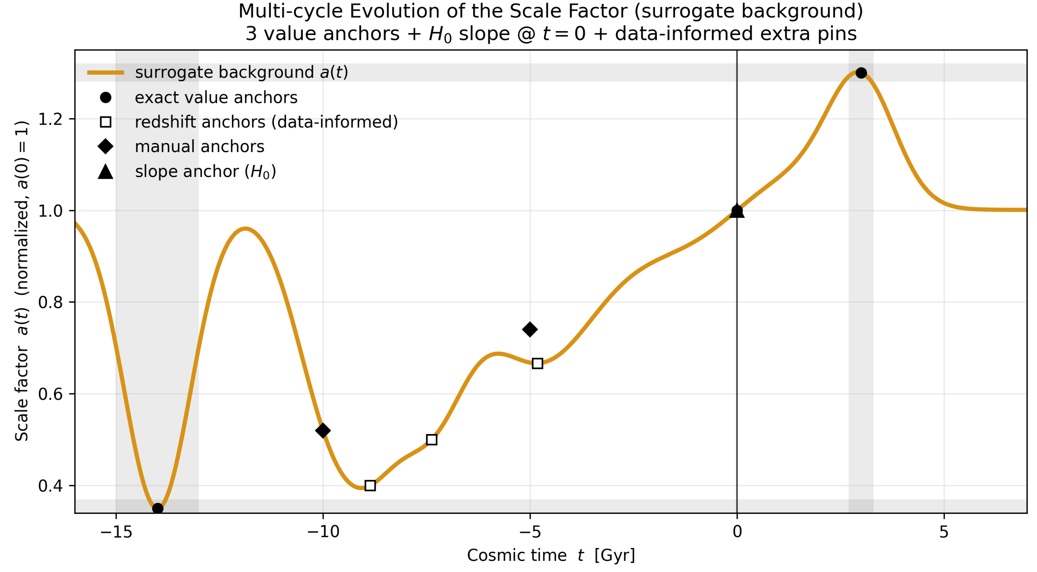
Figure 4.
Left: Transfer function for scalar perturbations across a symmetric QMM bounce. Right: Imprint power spectrum , exhibiting a mild blue tilt and UV cutoff. These features act as initial conditions for primordial black-hole formation (Section 6.2).
Figure 4.
Left: Transfer function for scalar perturbations across a symmetric QMM bounce. Right: Imprint power spectrum , exhibiting a mild blue tilt and UV cutoff. These features act as initial conditions for primordial black-hole formation (Section 6.2).
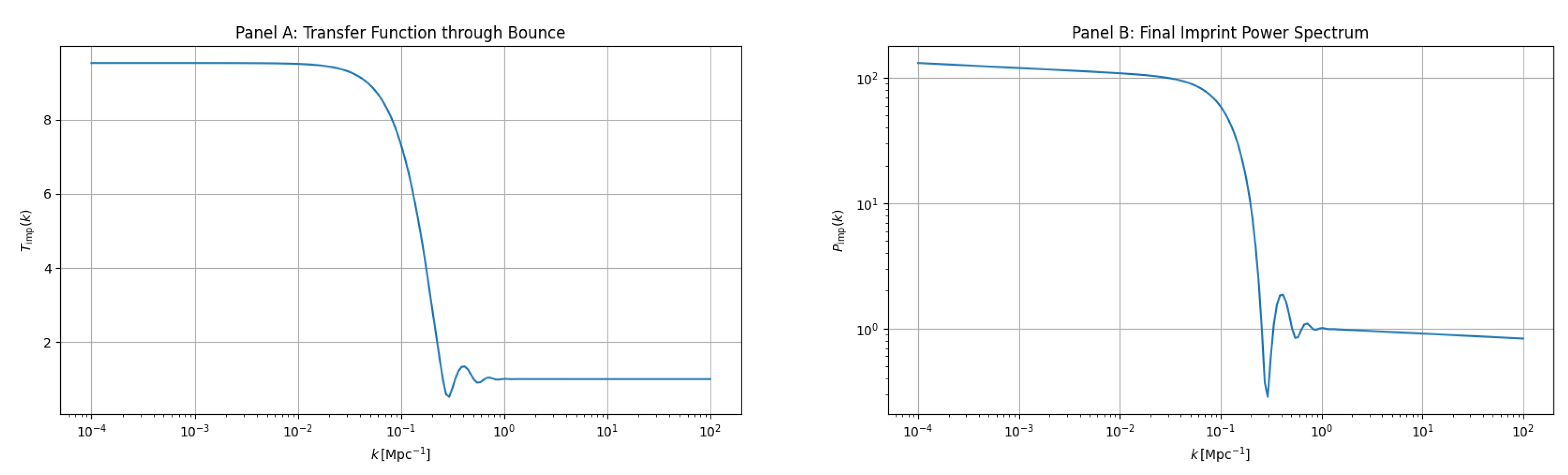
Figure 7.
Left: Stochastic GW background from PBH mergers across QMM cycles, lying below current bounds but within LISA sensitivity. Right: Posterior for the number of future cycles , combining entropy bounds with instability channels. Shaded bands: 68% and 95% credible intervals. All posteriors use the ODE background.
Disclaimer/Publisher’s Note: The statements, opinions and data contained in all publications are solely those of the individual author(s) and contributor(s) and not of MDPI and/or the editor(s). MDPI and/or the editor(s) disclaim responsibility for any injury to people or property resulting from any ideas, methods, instructions or products referred to in the content. |
© 2025 by the authors. Licensee MDPI, Basel, Switzerland. This article is an open access article distributed under the terms and conditions of the Creative Commons Attribution (CC BY) license (http://creativecommons.org/licenses/by/4.0/).
Copyright: This open access article is published under a Creative Commons CC BY 4.0 license, which permit the free download, distribution, and reuse, provided that the author and preprint are cited in any reuse.


