Submitted:
18 August 2025
Posted:
19 August 2025
You are already at the latest version
Abstract
We propose a new principle of adaptive Severe Plastic Deformation (SPD) processes, in which contact pressure stems from the reaction of the tool, rather than a force exerted on the workpiece externally. The reaction owes to special tool design utilizing a wedge effect. This approach ensures self-regulation of the deformation mode without the need for complex bidirectional loading systems. In addition, the equipment for adaptive processing can operate at loads which are substantially lower than those required for conventional SPD processing. Adaptability is analyzed by way of example for the High Pressure Sliding (HPS) process, for which theoretical justification, numerical calculations by the finite element method, and experimental verification are provided. It was established that, thanks to the self-regulation mechanism, the pressure is maintained automatically at the level necessary for plastic deformation of the workpiece. Experiments on copper samples showed the formation of an ultra-fine-grained structure. The results obtained demonstrate the efficacy of the adaptive HPS and open prospects for its application in the processing of thin-walled metal products.
Keywords:
Mechanical structure
; Severe Plastic Deformation
; High Pressure Sliding
; self-regulation
; Finite Element Simulation
; Ultrafine grained structure
1. Introduction
Severe Plastic Deformation (SPD) allows obtaining ultra-dispersive and heterostructured materials with excellent functional characteristics [1]. Among the various SPD methods, those designed for processing thin-walled samples, in which one of the dimensions is significantly smaller than the other two, occupy a special place [2]. High Pressure Torsion (HPT) [3] and High Pressure Sliding (HPS) [4] processes are used for sheet materials, High-Pressure Tube Twisting (HPTT) [2,5] or its continuous version [6] for tubes, and the Cone-Cone Method (CCM) [7] for shells.
Shear of a thin sample due to friction forces on its contact surfaces with the tool was first implemented by P. Bridgman in a device he invented [8], which became the prototype for modern HPT rigs. As friction hinders the spreading of the material, the compression of a thin sample creates pressure therein, which can exceed the yield stress substantially [9]. This leads to ‘seizure’ of the material by friction and causes its shearing. In terms of hydrostatic pressure and strain achieved, SPD processes for thin-walled samples significantly outperform other methods.
However, the implementation of such processes requires bidirectional equipment with the ability to dynamically control the forces during deformation. In one direction, a load is applied to provide contact pressure, and in the other, a force is applied to produce plastic deformation by shear. As the material hardens and the geometry of the sample changes, both forces must be adjusted, which complicates the design of the equipment. In addition, at a given pressure, the compressive force is proportional to the area of the sample and can reach several thousand tons for sheets with an area of about 100 cm2. Such apparatuses are unique and expensive, and their operation solely for creating a static force when processing relatively small workpieces can hardly be justified.
This paper proposes a different approach to manufacturing thin-walled products by severe plastic deformation. It is based on adaptive SPD processes, in which the contact pressure is created not by the active force of the press, but rather because of the reaction of the tool, realized by the wedge effect. This makes it possible to dispense with bidirectional equipment, significantly reduce the required press force when processing workpieces of a given size, and, for a given force, significantly increase the size of the workpieces that can be processed. Thanks to the underlying self-regulating mechanism, the reaction force automatically adapts to the mechanical properties and geometry of the workpiece, ensuring stable plastic deformation.
Adaptive feedback systems are traditionally associated with electronic control devices—sensors, controllers, and software. Modern approaches include neuro-fuzzy algorithms, machine learning, and real-time optimization, as discussed in detail in [10].
However, there is another class of systems where self-regulation is achieved through geometry, mechanics, and the structure of interactions of their constituent elements. Such solutions are widely used in automation, tribotechnology, and mechanical safety devices, demonstrating the system’s ability to adapt without the use of electronics.
A classic contribution in this field is provided in [11], which presents the first mathematical model of a mechanical regulator (governor) and formulates the conditions for the stability of a feedback system. The study demonstrates how the geometry and inertial properties of the regulator enable stabilization of a steam engine’s speed without external control.
Among the present-day studies, the work [12] is to be noted. The authors proposed an adaptive control system for Incremental Sheet Forming (ISF) where self-regulation is implemented by means of geometry of the sheet profile. In forming of curvilinear surfaces by this method the depth of deformation varies depending on the local inclination angle, which enables uniform stretching of the sheet. The control is based on the inbuilt geometric feedback and does not rely on electronic sensors, which makes it possible to boost the formability of the material without a need for external controls.
Article [13] discusses several microtube forming technologies that are inherently self-regulating. For example, diffusion-free drawing is based on localized heating and stretching, in which the deformation zone dynamically adapts to thermal and mechanical conditions without rigid tooling.
With this kind of adaptivity in mind, we focus specifically on mechanically implemented feedback as applied to SPD. We address the processes in which the pressure on the workpiece is formed and automatically adjusted not by external control, but by the internal response of a wedge system, which responds to changes in flow resistance of the deforming metal. The generic principle of adaptability is analyzed using the exemplary process HPS. For this case, the results of analytical modeling, numerical calculations, and experimental validation are presented. A similar approach can be applied to a broader range of SPD processes for thin-walled samples, such as HPT, HPTT, and CCM. However, specific design solutions for these processes are not discussed in this article, which is meant as a first introduction of the new process design paradigm.
2. Conceptual Framework of Adaptive Severe Plastic Deformation: Demonstration via High Pressure Sliding
Figure 1 shows a diagram explaining the adaptive HPS process based on the wedge effect. At the initial stage, a block comprising movable wedge elements W2, punch P, and metallic samples S1, S2 is placed between fixed wedge elements W1. Under the influence of gravity, the block sinks into the wedge gap, causing the occurrence of normal reaction force N₁ and friction force T₁ from W1. The resultant horizontal component of these forces presses the parts of the block together with a force N₂, while the static friction forces T₂ on the contact surfaces of the samples with elements W2 and P hold them together.
In the next stage of the process, the punch P is driven to move downward. If there is no slippage on the surface of the samples, its movement leads to further deepening of the blocks W1 into the wedge gap. This, in turn, gives rise to an increase in the force F required to move the punch, as well as an increase in the forces , and . This mode will continue until slippage occurs on the surfaces of the samples or until their plastic deformation sets in. Similar to the description of the HPT principle [2], to explain the self-regulating effect of HPS, we assume that the plastic deformation of the samples is caused exclusively by the action of tangential stresses to which hydrostatic pressure is applied. In the Discussion section, we will refine these ideas about the process by considering Non-Shear Flows, as was done for HPT in [14].
Let us consider the set of equations of equilibrium for the movable wedge element W2. The forces acting on it are shown in Figure 1. The equilibrium equations along the coordinate axes x and y read as follows:
The force caused by friction between the movable and fixed wedge elements is calculated using Coulomb’s formula for sliding friction force
where is the Coulomb friction coefficient corresponding to this contact surface.
After substituting relation (3) into the set of equations (1) and (2), one obtains:
It follows that
The force is caused by static friction between the sample and the elements adjacent to it (P and W2). Its maximum value corresponds to the sliding friction force = , which is determined by the pressure force . To prevent slippage on the sample surface, the force must satisfy the inequality:
To explain the principle of self-regulation, we assume that the maximum static friction force between the sample and the adjacent element of the tool is also described by Coulomb’s law, i.e.
where is the Coulomb friction coefficient corresponding to the contact surface between the sample and the tool.
In the Discussion section, we will explicate these ideas by considering that at high pressure on a plastically deformable body, Coulomb’s law ceases to apply, and the friction force reaches saturation [15].
Figure 2 illustrates the adaptive HPS process diagrammatically. It shows dependencies (6) and (8). The points on the straight line 1 represent the state of the process at any given moment in time. According to condition (7), if the representative point a is below the graph 2, there is no slippage of the punch and wedge elements on the sample surface.
Figure 2 shows that this condition is satisfied if the angle of inclination of the straight line 2 exceeds the angle of inclination of the straight line 1, i.e.
In this case, when the punch is moved downward, the block (W1, S1, P, S2, W1) is pressed as a single unit into the gap between the fixed wedge elements. This leads to an increase in forces and and the movement of the representative point (State Point) a along the graph 1 to point b, where it intersects the horizontal line 3, on which force induces plastic shear of the sample. Let us designate this point as Steady State Point, whose coordinates are .
The yield condition, which involves only the influence of tangential stresses on the onset of plastic flow of the material, has the form
where is the shear stress and is the yield stress of the material under shear.
It follows that
where is the surface area of the sample.
When a sample undergoes plastic shear, its material experiences strain hardening for a certain time and its surface area increases. This causes line 3 to shift upward. Point b shifts to the right, reflecting the increase in pressure on the sample, . The HPS process is always represented by point b. This is at the core of the principle of self-regulation, which consists in automatically maintaining the pressure force on the sample at a level sufficient for its plastic deformation.
Let us determine the pressure acting on the sample at the Steady State Point:
The force acting on the punch is determined from the equation of equilibrium along the y-axis and is equal to
If this force acted normally to the surface of sample, it would create a certain nominal pressure:
From equations (13) and (15), one obtains an expression for the pressure efficiency coefficient η
This coefficient quantifies the gain in the load efficiency of the adaptive HPS process over the conventional HPS and characterizes the lowering of the requirements on the equipment for processing. In the adaptive scheme, a single loading element enacting deformation of a workpiece is used. This is in contrast with the conventional process where two loading elements are necessary: one to produce pressure and the other for deforming the workpiece. Importantly, the pressure to be generated by the loading element in the adaptive process is by a factor of η lower than the one a much more powerful press must provide in the conventional process.
For small values of and , we assume and and obtain
For numerical estimation, let us set the values of the parameters at and [16]. Substitution of these values into Eq. (16) yields . In this case, it follows from condition (9) that no slippage on the surface of the samples will occur if .1.
In the following sections, we report the results of the application of the adaptive HPS process to severe plastic deformation of copper aiming at producing ultra-fine-grained thin-walled strips.
3. Materials and Methods
3.1. Experimental Rig for Adaptive HPS Process and Test Methodology
To realize the adaptive HPS process, an experimental rig was developed, a general view of which is shown in Figure 3. The setup is mounted on a 60-ton hydraulic press, which provides vertical movement of the movable plate at a controlled speed of 10 mm/s.
The main element of the setup is a wedge tool that provides contact pressure. The angle of inclination of the working surfaces of the wedges is 10°, which ensures sufficient force and stable operation of the setup. To reduce the friction coefficient and ensure stable deformation, coating of the working surfaces of the wedges with a graphite-based lubricant is used.
All elements directly involved in the deformation of the sample, i.e. the wedges and the punch, are made of tool steel hardened to a hardness of 56 HRC. This hardness ensures that the geometry of the tool is maintained at high contact pressures typical of SPD processes.
Copper strips M1 measuring 40 × 10 × 2 mm3 were used as samples. The process was carried out at room temperature.
Before deformation, the samples were subjected to heat treatment consisting in annealing at 550 °C for 1 hour, followed by cooling in water. This sample preparation ensured an initial homogeneous structure and reproducible conditions for SPD. The average microhardness of the initial samples was approximately 65HV.
Before an experiment, two samples were placed between the movable wedge elements (marked as W2 in Figure 1) and the punch. These elements were tightened with bolts, which allowed them to be securely pressed against the punch and fixed the samples in place. The resulting movable block with clamped samples was then placed in a rigid bandage with fixed wedges.
The deformation process was carried out by pressing the upper movable plate of the press onto the punch. Under the action of a vertical force, the movable block was inserted into the wedge gap of the bandage, causing relative displacement of the wedge elements W2 and shear deformation of the samples. The bolts connecting the wedge elements allow them to move towards the punch, ensuring uniform transmission of the reactive load. During the experiments, the punch was moved by 50 mm.
Upon completion of the process, the block with the samples was removed from the bandage and disassembled. The samples were carefully extracted for subsequent analysis of the microstructure and mechanical properties.
3.2. Methodology of Metallographic Study and Electron Backscatter Diffraction Experiments
Sample preparation for Electron Backscatter Diffraction (EBSD) measurements was conducted using a Struers LectroPol-5 electropolishing device with A2 electrolyte at an applied voltage of 20V. The EBSD measurements were performed on the surface of the sample, in its central zone, along its length using a Zeiss CrossBeam 350 SEM equipped with a Hikari Super EBSD camera. Orientation maps were acquired at an accelerating voltage of 10 kV using a 120 μm aperture. Maps were obtained at two magnifications: 1,000× with a step size of 500 nm, and 10,000× with a step size of 30 nm. Based on the EBSD data, the grain size distribution and misorientation angle distribution were analyzed for both the initial and deformed states. Data analysis was carried out using OIM Analysis™ 8 software.
3.3. Finite Element Calculation Method
The calculations were performed using the commercial software package QForm-3D (version QForm UK 10.3.1) [17], designed for modeling plastic deformation processes accounting for thermodynamic effects. The geometric model, material parameters, and loading modes were consistent with the actual experimental conditions.
The main assumptions and calculation conditions were as follows: planar deformation model was considered; deformation heating of samples was taken into account; sample material was assumed to be rigid-plastic, a representative stress-strain curve for Cu-OFE (99% Cu) was adopted; the tool was considered as an elastic body made of tool steel whose parameters correspond to a material with a hardness of 56 HRC; the plastic friction model for friction between the sample and the movable wedge was adopted, with the coefficient of friction equal to 1; for friction between the movable and fixed wedges a model based on Coulomb’s law was adopted, with a friction coefficient of 0.05, which corresponds to the use of graphite lubricant, as in the experiment; finally, room temperature conditions without additional external heating were considered.
Computational mesh comprised about 10,000 finite elements, providing sufficient accuracy in the region of strain localization. An implicit integration algorithm was used to ensure stability and accuracy of the calculations for the process considered, which involves strong nonlinearity. The remaining parameters (mesh adaptation intervals, convergence criteria, time integration, and plasticity control) were set automatically according to QForm recommendations and did not require additional configuring.
4. Results
4.1. Results of Finite Element Method Calculations
The purpose of the calculations using the finite element method was to demonstrate the principle of adaptability exemplified by the High Pressure Sliding (HPS) process. Particular attention was focused on verifying the key mechanism—the formation and dynamic maintenance of the conditions necessary for the realization of sufficiently large shear strain in the samples.
Figure 4 shows graphs of the time dependence of the pressure forces on the punch and the sample, as well as the displacements of the punch and the movable wedges.
The calculations show that as the punch moves, the force acting on it rises. This is due to a combined effect of the strain hardening of the sample material and the increase in its contact area with the tool. At the same time, there is a coordinated movement of the wedge elements, which leads to an increase in pressure on the sample. We emphasize again that this happens without any external control — which is fully in line with the self-regulation mechanism outlined in Section 2. Thus, the FEM-based numerical experiment confirms that the insertion of the punch activates the wedge system, which automatically raises the pressure on the sample and maintains a stable mode of plastic deformation. The maximum compressive force acting on the sample exceeds the force required for moving the punch by a factor greater than 2. This result is consistent with the magnitude of the pressure efficiency coefficient η, defined in Section 2.
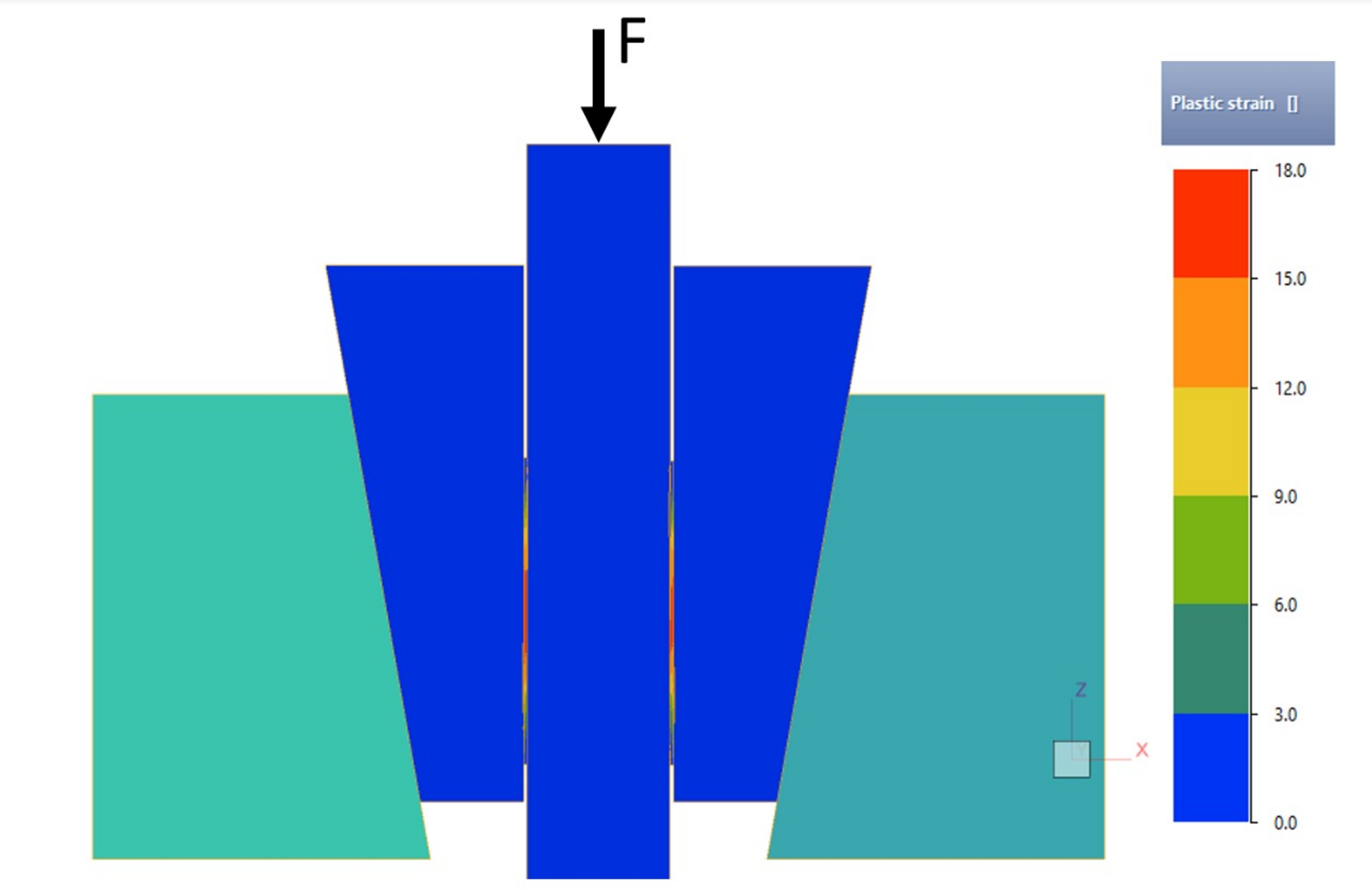
Figure 5 shows the results of numerical simulations illustrating the spatial distribution of the equivalent von Mises plastic strain and hydrostatic pressure in the sample in the final stage of the adaptive High Pressure Sliding (HPS) process. Figure (a) shows the distribution of the equivalent von Mises plastic strain (effective strain), denoted , throughout the sample, and (b) shows an enlarged area of the middle zone of the sample, highlighted in (a) with a dotted frame. The calculation shows that in the middle part of the sample, reaches values of 15-18, which qualifies this process as a Severe Plastic Deformation technique.
Figure 5.
Distributions of the equivalent von Mises plastic strain and hydrostatic stress σ in the M1 copper sample in the final stage of the adaptive High Pressure Sliding process: (a) equivalent von Mises strain field; (b) enlarged area of the middle part of the sample (delineated in (a) with a dotted rectangle); (c) distribution of hydrostatic pressure in the same area.
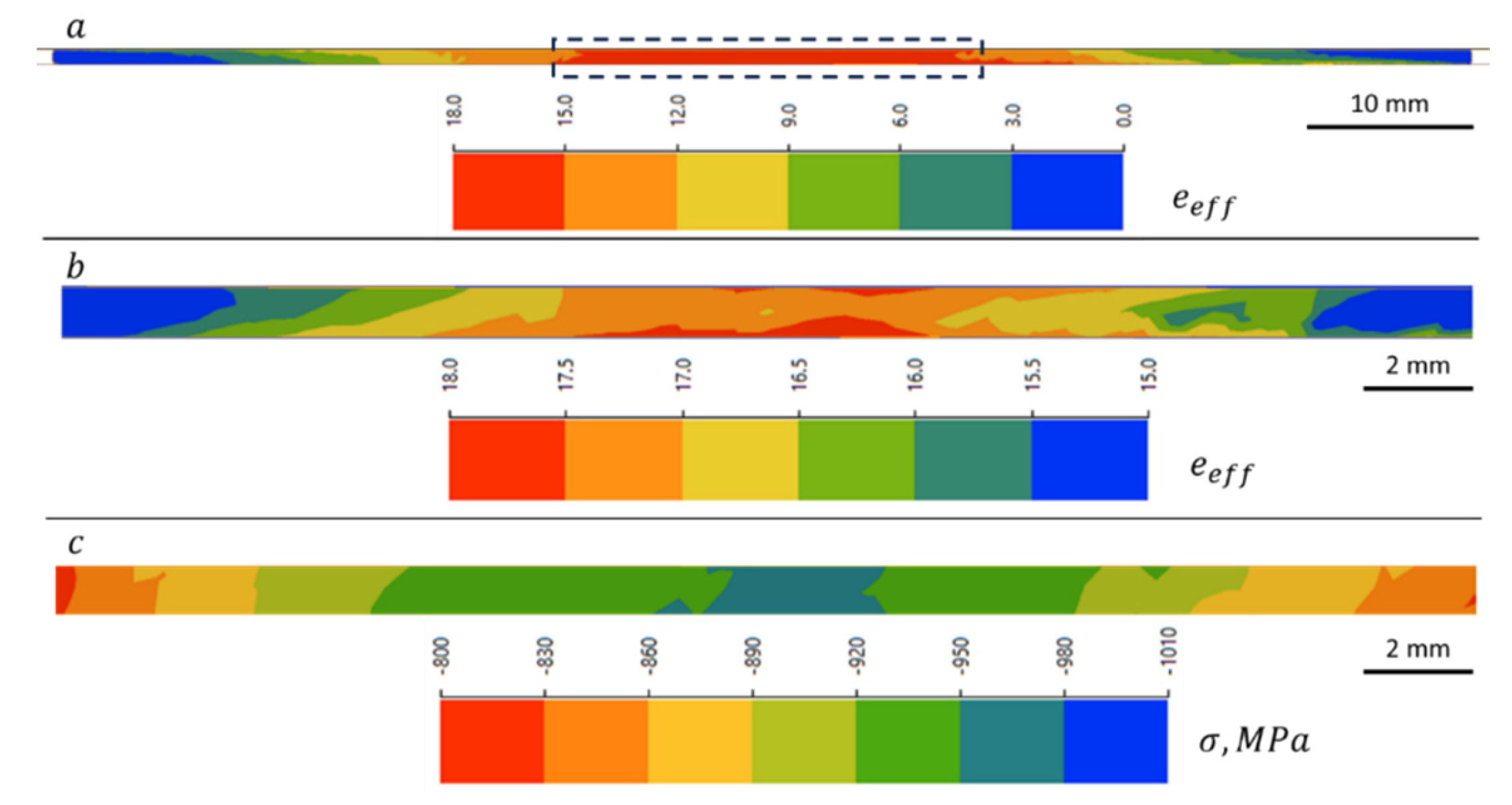
Figure 5c displays the distribution of hydrostatic stress in the middle zone of the sample. The hydrostatic pressure reaches 1010 MPa, and the average value is approximately 900 MPa, which is 2.6 times higher than the plastic flow stress of 345 MPa in this area at the final stage of deformation. Such high pressure confirms the effective activation of the self-regulation mechanism: the sample experiences powerful compression, which stabilizes the plastic deformation process.
Numerical FEM simulations demonstrated that, thanks to the self-regulation effect occurring in the wedge system, the contact pressure adapts to the mechanical characteristics and geometry of the deforming sample that vary during HPS in keeping with the adaptive processing concept we propose.
4.2. Results of Microstructure Investigation
Analysis of the microstructure of the material before and after adaptive HPS demonstrates significant changes resulting from intense plastic deformation. The data obtained includes optical images, EBSD maps, and quantitative histograms reflecting the evolution of the structure and the nature of the boundaries.
The photographs of the sample before and after HPS (Figure 6) clearly show its significant deformation.
Unlike simple compression, which would mainly result in deformation across the sample width [18], the inclusion of a shear component enables more uniform processing of the bulk of the material. This is confirmed by the observed change in the shape of the sample.
Figure 7 presents a comprehensive characterization of the microstructure of the initial material based on EBSD analysis.
The orientation map (a) shows a coarse-grained structure with a pronounced presence of twin boundaries. Most of the boundaries are Σ3 boundaries with a characteristic misorientation of about 60°, which is typical for metals with a face-centered cubic (FCC) lattice. The boundary map (b) confirms the predominance of twins, as well as the presence of low-angle boundaries (3°–10°), indicating substructures formed as a result of previous thermomechanical treatment.
The grain size distribution histogram (c) shows that the average grain diameter is approximately 19.7 μm. The misorientation angle distribution (d) exhibits a pronounced peak at 60°, corresponding to twin boundaries, and a moderate presence of low-angle boundaries. The direct pole figure (e) demonstrates the absence of a pronounced crystallographic texture—the distribution of points is uniform, without any clearly pronounced concentrations, which indicates a random orientation of grains in the volume.
Thus, the initial state is characterized by a recrystallized coarse-grained structure with a high proportion of twins and an isotropic distribution of crystallographic orientations.
Figure 8 illustrates the microstructural characteristics of the material after the adapted HPS process.
The EBSD orientation map (a) shows the formation of an ultra-fine-grained (UFG) structure. The average grain size dropped to ~385 nm, which is confirmed by the histogram (d). The boundary map (c) shows a significant increase in the proportion of high-angle boundaries (>10°) not related to twins, indicating that originally non-textured material evolved towards a textured one and suggesting activation of dynamic recrystallization mechanisms.
The histogram (e) shows a redistribution of misorientation angles: the peak at 60° became much less pronounced, and the proportion of high-angle boundaries rose. This indicates the destruction of twins and the formation of a new grain boundary network. In contrast to the initial state, the direct pole figure (f) demonstrates the presence of a crystallographic texture—the concentration of points indicates the preferred orientations of the grains formed during the deformation process. The detailed analysis of EBSD data reveals the preponderance of the S-type texture component ({123}<634>), which is characteristic of severe shear deformation. This points to high dislocation activity and grain rotation, typical of the high strain levels introduced by severe plastic deformation in FCC metals. The development of this texture may also be influenced by dynamic recrystallization processes, which contribute to grain refinement while preserving or enhancing shear-related orientations.
Thus, the adaptive HPS process leads to a profound transformation of the microstructure expressed as extreme grain refinement, an increase in the proportion of high-angle boundaries, and the formation of a textured UFG structure.
5. Discussion
While the results reported above provide convincing proof of concept for the adaptive SPD principle we would like to promulgate, two important limiting factors not taken into account in Section 2 need to be considered. The first factor is the deviation of the friction force from Coulomb’s law and its saturation at high pressures. The second is the influence of pressure on the plastic shear of the sample.
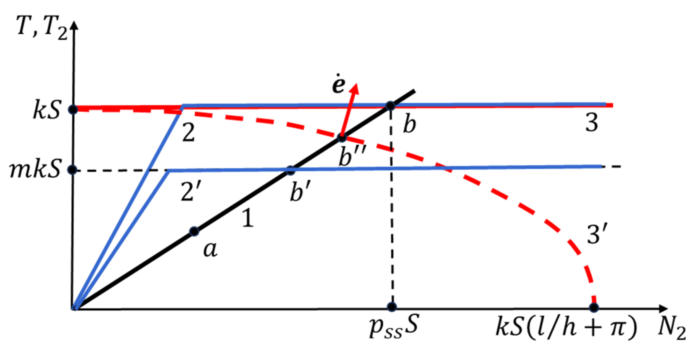
Figure 9 shows a refined diagram of the process analysis that does account for the above factors. It should be considered vis-à-vis Figure 2 used in the foregoing sections.
As distinct from the diagram in Section 2, in this refined diagram the function reaches saturation at sufficiently large values of . This is shown schematically by a broken line consisting of a straight inclined section reflecting the growth of and a horizontal straight line corresponding to the saturation level. This behavior of corresponds to the results of studies of contact friction in metal forming processes. According to [19], at high pressures , the friction stress is determined by the relation
where is the coefficient of friction.
Figure 9 shows two forms of the dependence corresponding to dry friction (, straight line 2) and lubricated surfaces (, straight line 2’).
To include the effect of the pressure force on the plastic deformation of the sample, it is necessary to consider a more general condition of plasticity instead of relation (10). It is obtained by following the generalized variables approach [20], considering the tangential stress and the average contact pressure as generalized loads. The generalized rates associated with them enter the expression for the specific power of plastic deformation:
where is the shear strain rate and is the strain rate along the sample length.
According to the generalized variables approach, it follows from (19) that is the generalized rate conjugate to and is the generalized rate conjugate to . In this case we have:
where λ is the proportionality coefficient, and is the plastic potential, through which the generalized condition of plasticity is formulated:
When the material remains in an elastic state.
As is customary in the literature (see [21]), the potential can be represented as
The coefficients and entering this equation can be found by considering two limiting cases. In the first case, the sample is loaded only with shear stresses, i.e., . In this case, the generalized plasticity condition has the form:
Comparing this equation with condition (10), we obtain:
Let us now consider the case when the sample is loaded only by normal pressure, i.e. . In this case, the generalized plasticity condition takes the form:
According to [9], the average pressure on a thin strip causing its plastic flow is determined by the parameter
where and are the length and thickness of the strip, respectively.
Equation (27) was obtained under the assumption that and there is limiting friction on the surface of the strip. From Eqs. (26) and (27) it follows:
Substituting the above expressions for and into (23), we obtain:
The generalized plasticity condition (22) thus takes the following form:
Multiplying both sides of this equation by the surface area of the sample, , we obtain the plasticity condition in terms of the variables and :
This ratio determines the Generalized Plasticity Locus in the first quadrant of the plane in the form of a quarter ellipse, whose minor axis is equal to and major axis is equal to (see Figure 9, curve 3’).
We can now apply the diagram in Figure 9 to analyze the possible modes of the adaptive process.
First of all, we note that in the case when the dry friction mode is not realized on the surface of the sample (when ), a steady state occurs at point , corresponding to the intersection of the curve with the straight line 1. Since this point lies within the area bounded by the Generalised Plasticity Locus, the sample is not subjected to plastic deformation, and the punch slips over its surface.
In dry friction (m=1), the representative point (‘State Point’) of the process moves along the straight line 1 to point , where the latter intersects the Generalised Plasticity Locus. At this moment, plastic deformation of the sample begins, including both the shear component , and the thickness deformation . According to relation (20), the shear deformation rate is proportional to the projection of the normal vector onto the Generalised Plasticity Locus on the axis, and according to relation (21), is proportional to the projection of this vector onto the axis, but with the opposite sign. From Figure 9, it follows that at point the inequality is satisfied, i.e., plastic deformation is accompanied by a decrease in the thickness of the sample and an increase in its transverse dimensions. As a result, the major semi-axis of the ellipse (30) gets elongated, and the generalized plasticity surface ( 3’ ) expands, approaching its limit position — a straight line ( 3 ) that appears when . At the same time, point shifts in the direction of point , and the normal vector rotates, getting closer and closer to the direction of the axis. This is accompanied by an increase in its projection onto the specified axis and a decrease in the projection onto the axis, which means an increase in the share of shear deformation and a decrease in the share of deformation across the thickness of the sample. In the limit of , the deformation of the sample is carried out only by shear.
The analysis shows that the refined model of the High Pressure Sliding adaptive process allows new deformation modes to be identified, but its key feature remains unchanged: thanks to the wedge feedback mechanism, the contact pressure is automatically adjusted to the value required for plastic deformation of the sample. The simple shear mode under pressure predicted by the simplified model is realized as a limiting case at large strains.
6. Conclusions
This study demonstrates that the wedge geometry of the tool can be effectively used to generate contact pressure during severe plastic deformation. This approach enables the realization of a self-regulating mode in which the pressure is automatically maintained at a level sufficient for plastic flow of the material, regardless of its geometry and hardening stage. An important advantage of the adaptive process is that no special loading element is needed to produce pressure on the workpiece. Moreover, the load required to operate the principal loading element is just a fraction of that involved in the conventional HPS. This makes it possible to conduct adaptive HPS using equipment with a significantly lower load capacity, which simplifies the design of the processing rigs and broadens the range of industry-scale applications of HPS processing.
An analytical model based on equilibrium equations and generalized plasticity conditions made it possible to determine the conditions for the feasibility of the adaptive process. Numerical calculations using the finite element method helped determining the force conditions of the process and the amount of effective (equivalent) strain in the sample. The EBSD results obtained revealed a transition from a coarse-grained structure to an ultra-fine-grained state with an increased proportion of high-angle boundaries. It was found that the microhardness in the deformation zone increased more than threefold, up to approximately HV 200.
Although in this work the principle of adaptability was analyzed using the example of the High Pressure Sliding (HPS) process, it is also applicable to other SPD processes designed for processing thin-walled bodies of various geometries. In particular, similar mechanisms can be implemented in modified versions of the High Pressure Torsion (HPT), High-Pressure Tube Twisting (HPTT), and Cone-Cone Method (CCM), where it is also possible to use reactive forces arising from the directed movement of the tool in a closed or wedge-shaped system.
Specific design implementations of adaptable versions of these processes are beyond the scope of this article and will be presented separately. Nevertheless, the general idea of using self-regulating pressure arising from the interaction between the tool and the resistance of the material can serve as the basis for the development of a wide class of effective SPD processes.
Author Contributions
Conceptualization, Y.B.; methodology, O.D., G.B., S.K., and M.M.; validation, Y.B., O.D., S.K., and Y.E.; formal analysis, Y.B. and Y.E.; investigation, O.D., G.B., S.K., M.M., and S.M.; resources, G.B.; data curation, O.D., M.M., and S.M.; writing—original draft preparation, Y.B., O.D., and M.M.; writing—review and editing, Y.E.; visualization, O.D., S.K., M.M., and S.M.; supervision, Y.B.; project administration, Y.B.; funding acquisition, Y.B., O.D., G.B., S.K., and M.M. All authors have read and agreed to the published version of the manuscript.
Funding
This research received no external funding.
Data Availability Statement
The data supporting the findings of this study are available from the corresponding author upon reasonable request.
Acknowledgments
YB would like to thank the Polish National Agency for Academic Exchanges (NAWA) for financial support of this work within the Ulam NAWA program (Decision No. BNI/ULM/2024/1/00008/DEC/I), project "Heterostructure formation in metals by Rotating Indenter Technique". The authors deeply appreciate the support of MICAS Simulations Ltd., Oxford, UK, for generously providing the QForm-3D software suite (version QForm UK 10.3.1) for finite-element analysis.
Conflicts of Interest
The authors declare no conflicts of interest.
Abbreviations
The following abbreviations are used in this manuscript:
| SPD | Severe Plastic Deformation |
| HPT | High Pressure Torsion |
| HPS | High Pressure Sliding |
| HPTT | High-Pressure Tube Twisting |
| CCM | Cone-Cone Method |
References
- Segal, V. Review: Modes and Processes of Severe Plastic Deformation (SPD). Materials 2018, 11, 1175. [Google Scholar] [CrossRef] [PubMed]
- Lapovok, R.; Pougis, A.; Lemiale, V.; et al. Severe plastic deformation processes for thin samples. J. Mater. Sci. 2010, 45, 4554–4560. [Google Scholar] [CrossRef]
- Kawasaki, M.; Figueiredo, R.B.; Langdon, T.G. Recent Developments in the Processing of Advanced Materials Using Severe Plastic Deformation. Mater. Sci. Forum 2021, 1016, 3–8. [Google Scholar] [CrossRef]
- Fujioka, T.; Horita, Z. Development of High-Pressure Sliding Process for Microstructural Refinement of Rectangular Metallic Sheets. Mater. Trans. 2009, 50, 930–933. [Google Scholar] [CrossRef]
- Tóth, S.; Arzaghi, M.; Fundenberger, J.J.; Beausir, B.; Bouaziz, O.; Arruffat-Massion, R. Severe plastic deformation of metals by high-pressure tube twisting. Scr. Mater. 2009, 60, 175–177. [Google Scholar] [CrossRef]
- Lapovok, R.; Qi, Y.; Ng, H.P.; Toth, L.S.; Estrin, Y. Gradient Structures in Thin-Walled Metallic Tubes Produced by Continuous High Pressure Tube Shearing Process. Adv. Eng. Mater. 2017, 19, 1700345. [Google Scholar] [CrossRef]
- Bouaziz, O.; Estrin, Y.; Kim, H.-S. Severe plastic deformation by the cone-cone method: potential for producing ultrafine grained sheet material. Rev. Métall. 2007, 104, 318–322. [Google Scholar] [CrossRef]
- Bridgman, P.W. Effects of high shearing stress combined with high hydrostatic pressure. Phys. Rev. 1935, 48, 825–847. [Google Scholar] [CrossRef]
- Kachanov, L.M. Fundamentals of the Theory of Plasticity; Dover Publications: Mineola, NY, USA, 2004. [Google Scholar]
- Mohammadzadeh, A.; Sabzalian, M.H.; Zhang, C.; Castillo, O.; Sakthivel, R.; El-Sousy, F.F.M. Modern Adaptive Fuzzy Control Systems; Springer: Cham, Switzerland, 2023. [Google Scholar] [CrossRef]
- Maxwell, J.C. On Governors. Proc. R. Soc. Lond. 1868, 16, 270–283. [Google Scholar] [CrossRef]
- Nirala, H.K.; Agrawal, A. Adaptive increment based uniform sheet stretching in Incremental Sheet Forming (ISF) for curvilinear profiles. J. Mater. Process. Technol. 2022, 306, 117610. [Google Scholar] [CrossRef]
- Hartl, C. Review on Advances in Metal Micro-Tube Forming. Metals 2019, 9, 542. [Google Scholar] [CrossRef]
- Beygelzimer, Y.; Estrin, Y.; Davydenko, O.; Kulagin, R. Gripping Prospective of Non-Shear Flows under High-Pressure Torsion. Materials 2023, 16, 823. [Google Scholar] [CrossRef] [PubMed]
- Nielsen, C.V.; Bay, N. Review of friction modeling in metal forming processes. J. Mater. Process. Technol. 2018, 255, 234–241. [Google Scholar] [CrossRef]
- Muzakkir, S.M.; Hirani, H.; Thakre, G.D. Lubricant for Heavily Loaded Slow-Speed Journal Bearing. Tribol. Trans. 2013, 56, 1060–1068. [Google Scholar] [CrossRef]
- QForm 3D. Metal Forming Simulation Software; M.S. Limited: 2024. Available online: https://www.qform3d.com.
- Johnson, W.; Mellor, P.B. Engineering Plasticity; Ellis Horwood Ltd.: Chichester, UK, 1983. [Google Scholar]
- Levanov, A.N.; Kolmogorov, V.L.; Burkin, S.P.; Kaztac, B.R.; Ashpuz, V.; Spassky, I. Contact friction in metal forming processes. Metallurgia USSR 1976, 416. (In Russian) [Google Scholar]
- Prager, W.; Hodge, P.G. Theory of Perfectly Plastic Solids; John Wiley & Sons: New York, NY, USA; Chapman & Hall: London, UK, 1951. [Google Scholar]
- Rabotnov, Y.N. Mechanics of Deformable Solids; Nauka: Moscow, Russia, 1979. (In Russian) [Google Scholar]
Figure 1.
Diagram explaining the principle of operation of the adaptive HPS. The figure shows: W1 – fixed wedge elements; W2 – movable wedge elements; P – punch; S1, S2 – samples of the material being processed; –normal and tangential forces acting on W2 on the contact surfaces with W1; –normal and tangential forces acting on W2 on the contact surfaces with the samples; F – force applied to the punch.
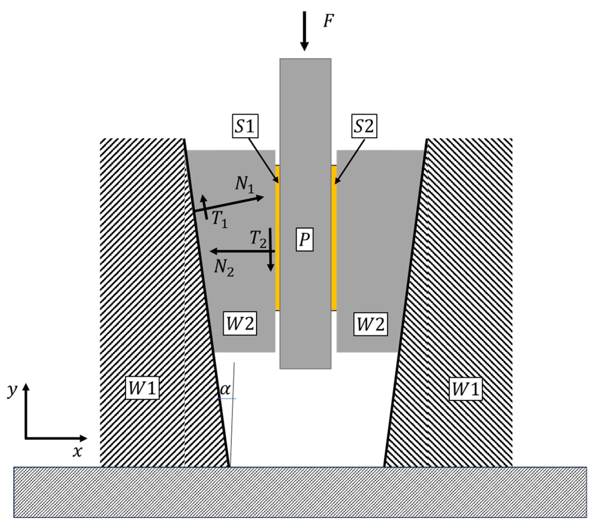
Figure 2.
Graphic representation of the analysis of the adaptive HPS process. 1- graph of the function according to relation (6); 2- graph of the function according to relation (8); 3- plastic shear limit; a – representative point corresponding to the state of the process; b- Steady State Point. Here S and k denote the surface area of the sample and the yield stress under shear deformation, respectively.
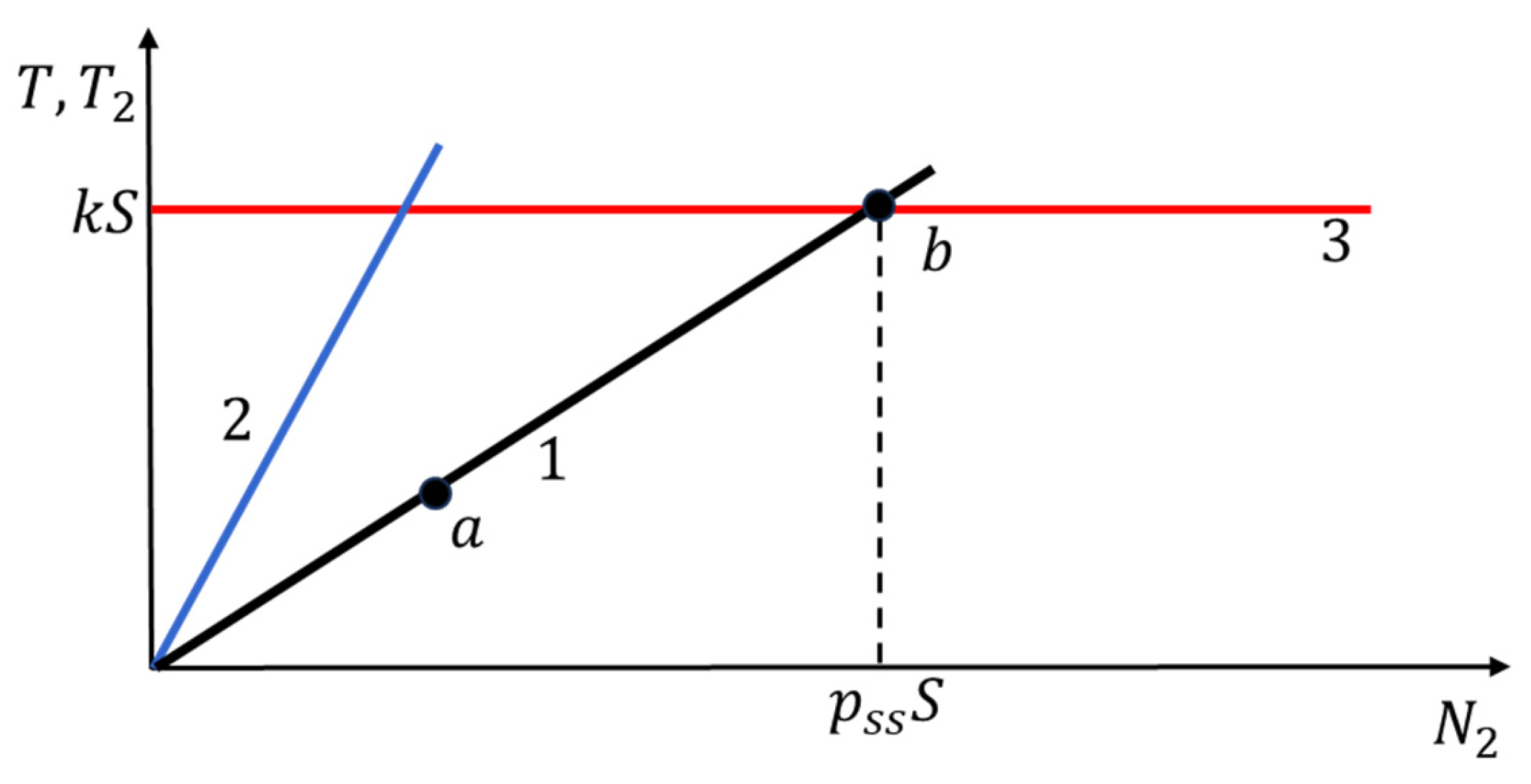
Figure 3.
Photo of the adaptive HPS process rig employed.
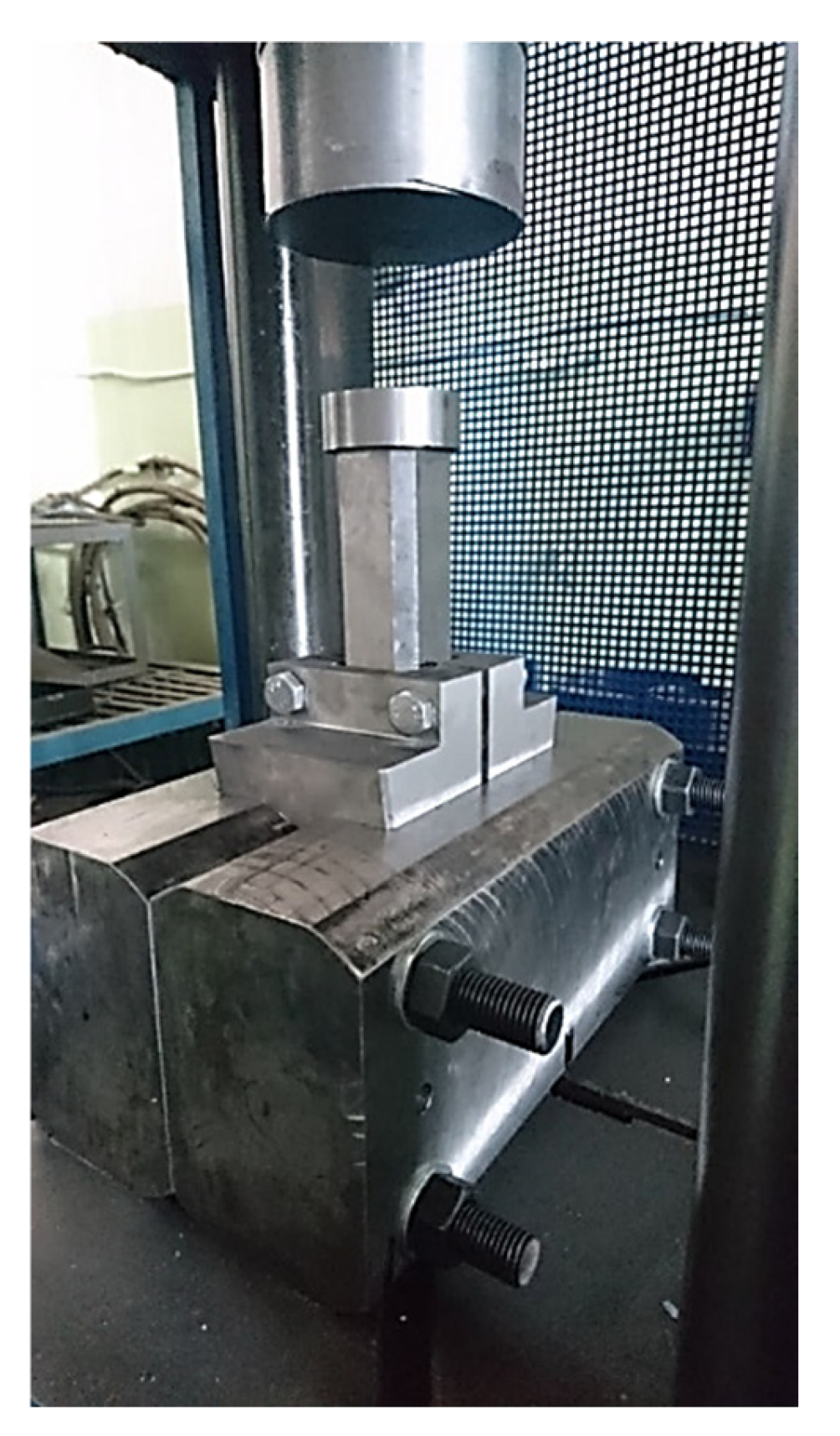
Figure 4.
Graphs showing the dependence of the pressure forces on the punch and the sample on time, as well as the displacements of the punch and movable wedges. The notation used is as follows: 1 - force acting on punch P; 2 - projection of the force on the axis (the compressive force acting on the sample); 3 – displacement of punch P; 4 – displacement of the mobile wedge element W2 (cf. Figure 1).
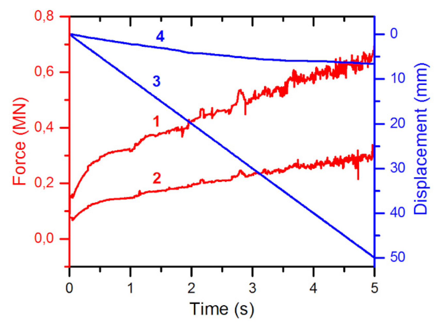
Figure 6.
Photographs of the sample: (a) before and (b) after the adaptive HPS process. The circle in image (b) indicates the area in which the microstructural study was conducted. The microhardness in this area was approximately 200 HV.
Figure 6.
Photographs of the sample: (a) before and (b) after the adaptive HPS process. The circle in image (b) indicates the area in which the microstructural study was conducted. The microhardness in this area was approximately 200 HV.
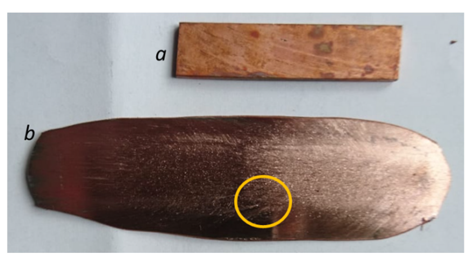
Figure 7.
EBSD analysis of the source material: (a) orientation map; (b) map of boundaries with color coding by misorientation angles; (c) grain size distribution (average grain size ~19.7 μm); (d) distribution of crystallographic misorientation angles with a pronounced peak at 60°, corresponding to twin boundaries; (e) direct pole figure demonstrating the absence of pronounced crystallographic texture.
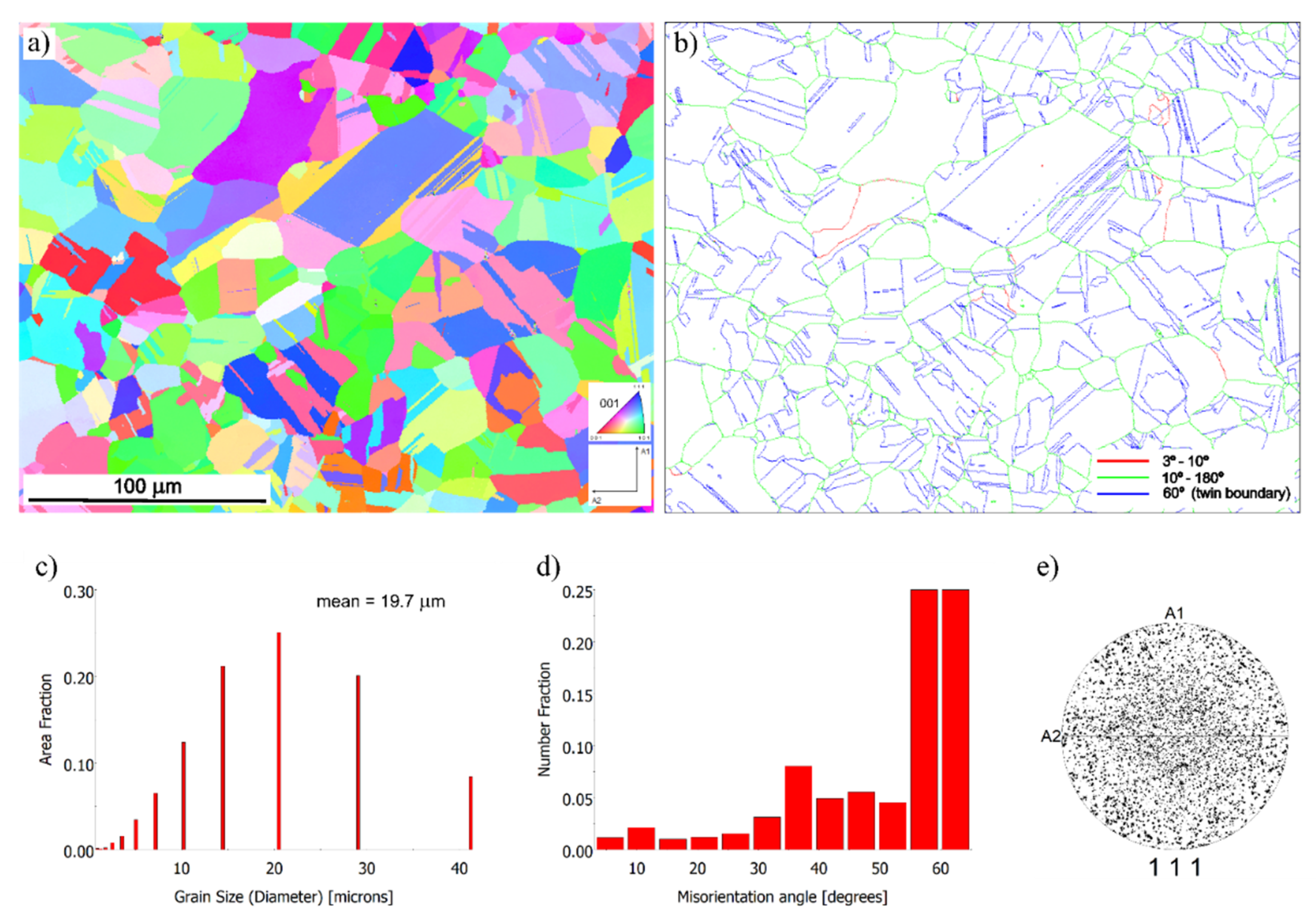
Figure 8.
EBSD analysis of the material after adaptive HPS: (a, b) orientation maps obtained at lower and higher magnifications, respectively; (c) boundary map with a predominance of high-angle boundaries; (d) grain size distribution (average grain size ~385 nm); (e) misorientation angle distribution; (f) direct pole figure demonstrating the formation of crystallographic texture as a result of deformation.
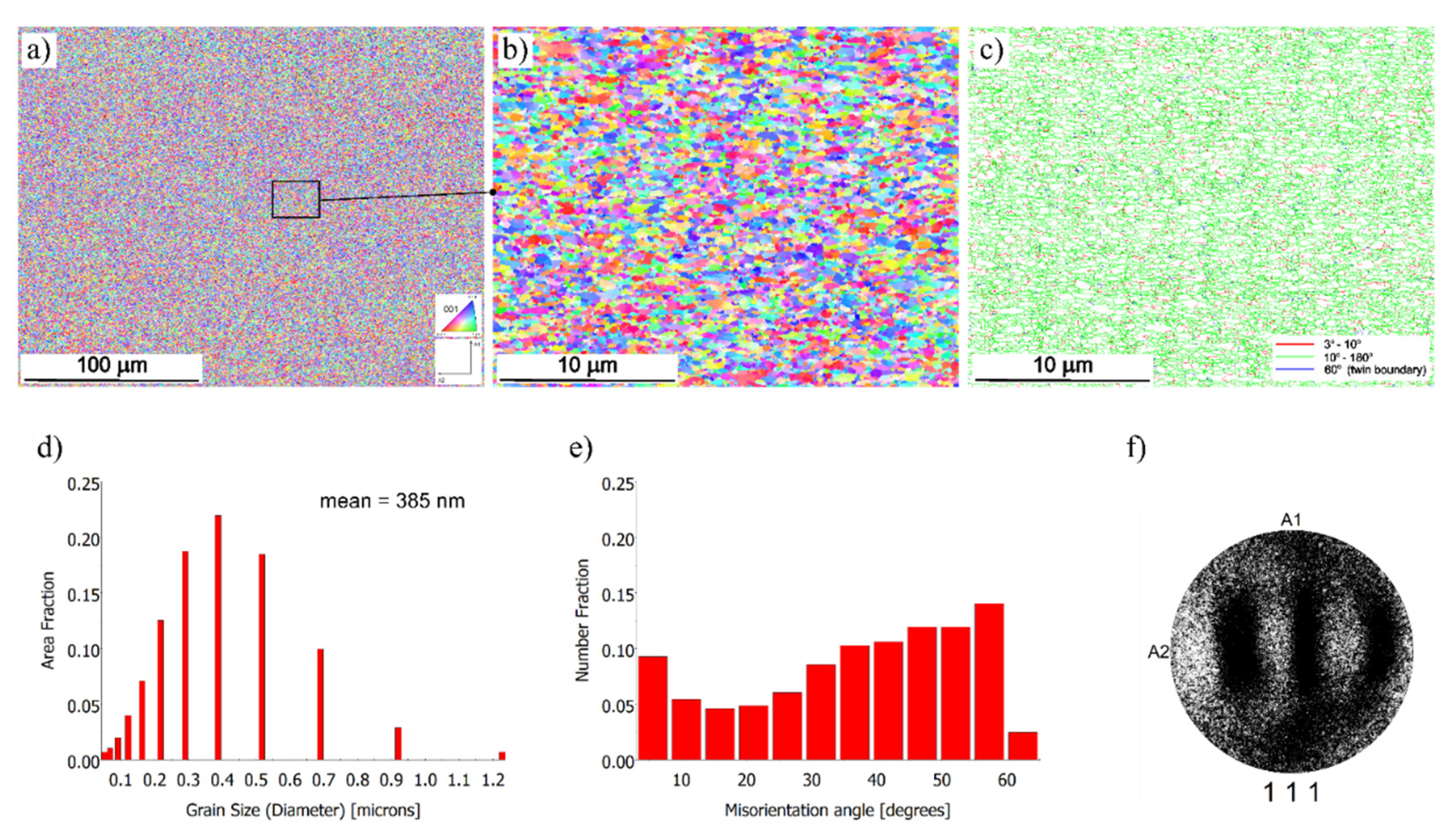
Figure 9.
Refined diagram of the analysis of the modes of the adaptive HPS process. 1- graph of the function according to relation (6); 2 and 2’—graphs of the function for dry friction (2) and for friction with lubrication (2’); 3—plastic shear limit of the sample under the action of tangential stresses only; a – representative point corresponding to the state of the process; b- Steady State Point.
Disclaimer/Publisher’s Note: The statements, opinions and data contained in all publications are solely those of the individual author(s) and contributor(s) and not of MDPI and/or the editor(s). MDPI and/or the editor(s) disclaim responsibility for any injury to people or property resulting from any ideas, methods, instructions or products referred to in the content. |
© 2025 by the authors. Licensee MDPI, Basel, Switzerland. This article is an open access article distributed under the terms and conditions of the Creative Commons Attribution (CC BY) license (http://creativecommons.org/licenses/by/4.0/).
Copyright: This open access article is published under a Creative Commons CC BY 4.0 license, which permit the free download, distribution, and reuse, provided that the author and preprint are cited in any reuse.


