
Submitted:
14 August 2025
Posted:
15 August 2025
You are already at the latest version
Abstract
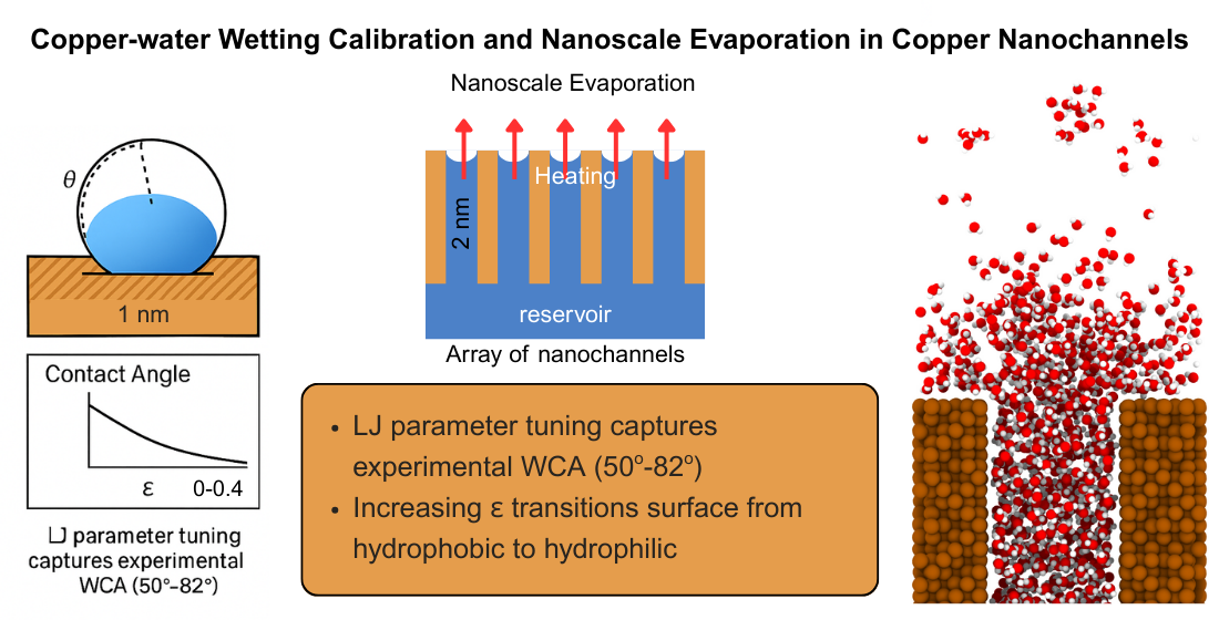
This study presents a molecular dynamics (MD) investigation of water evaporation in copper nanochannels, with a focus on accurately modeling copper–water interactions through force-field calibration. The TIP4P/2005 water model was coupled with the Modified Embedded Atom Method (MEAM) for copper, and the oxygen–copper Lennard–Jones (LJ) parameters were systematically tuned to match experimentally reported water contact angles (WCA) on Cu(111) surfaces. Contact angles were extracted from simulation trajectories using a robust five-step protocol involving 2D kernel density estimation, adaptive thresholding, circle fitting, and mean squared error (MSE) validation. The optimized force field demonstrated strong agreement with experimental WCA values (50.2°–82.3°), enabling predictive control of wetting behavior by varying ε in the range 0.20–0.28 kcal/mol. Using this validated parameterization, we explored nanoscale evaporation in copper channels under varying thermal loads (300–600 K). Results reveal a clear temperature-dependent transition from interfacial-layer evaporation to bulk-phase vaporization, with evaporation onset and rate governed by the interplay between copper–water adhesion and thermal disruption of hydrogen bonding. These findings provide atomistically resolved insights into wetting and evaporation in metallic nanochannels, offering a calibrated framework for simulating phase-change heat transfer in advanced thermal management systems.
Keywords:
MD simulation
; TIP4P/2005
; Contact angle
; nanochannel evaporation
; wetting behavior
; MEAM potential
; nanoconfined water
1. Introduction
Recent advancements in machine learning and computational modeling have significantly impacted nuclear energy research, particularly in the areas of reactor monitoring, safety assessment, and thermal-hydraulic analysis. Studies have demonstrated the feasibility of using multisource sensor data with limited labels for power level classification in nuclear reactors [1], and innovative frameworks integrating machine learning with uncertainty quantification have improved fire risk assessment in nuclear facilities [2]. Soft computing techniques, including neural networks and fuzzy systems, have also found broad applications in reactor diagnostics, heat transfer, and safety evaluation [3]. In high-fidelity reactor simulations, reduced-order modeling (ROM) approaches—such as convolutional neural networks and the Non-Linear Independent Dual System (NIDS)—have enhanced the efficiency of neutron transport modeling [4]. Likewise, ML-driven rapid prediction of multiphysics coupled fields has been applied to small modular reactors such as lead-cooled fast reactors (LFRs), improving real-time thermal analysis [5]. Furthermore, hybrid data-driven and physics-informed ML methods have been successfully used to model thermal-hydraulic behavior in geological nuclear waste repositories [6]. In this context, our study offers valuable insights into nanoscale phase change and interfacial heat transfer, which are critical for the thermal management of advanced nuclear systems, including microreactors and compact heat exchangers. By bridging molecular-level evaporation phenomena with macroscale energy systems, this work complements ongoing efforts to enhance the predictive capabilities and safety margins of next-generation nuclear technologies.
Nanoscale evaporation plays a critical role in thermal management systems for nuclear energy applications [9,13], where efficient phase-change heat transfer in micro-coolant channels directly impacts reactor safety and performance. When water is confined at this scale, conventional continuum models break down due to dominant surface interactions, non-equilibrium behaviors, and size effects that invalidate macroscopic assumptions [10]. Molecular dynamics simulations have therefore become essential for probing evaporation mechanisms [15], with atomistic models like TIP4P offering high fidelity through explicit treatment of hydrogen bonding and electrostatics [7,8]. This computational approach captures water's profoundly altered behavior under nanoconfinement, where geometric restrictions induce layered molecular structuring [10], while confinement dimensions and surface chemistry dictate anomalous density distributions, diffusion rates, and hydrogen-bonding patterns [14].
Despite extensive research on water interactions with carbonaceous materials like graphene and carbon nanotubes [11,15], metal-water interfaces remain significantly understudied [12]. This knowledge gap is particularly concerning given copper's ubiquity in nuclear heat exchangers, steam generators, and containment systems. The scarcity of studies on copper-water interfaces stems partly from challenges in force-field parameterization, where inaccuracies in modeling van der Waals interactions can misrepresent interfacial wettability and evaporation dynamics [14]. Recent work has addressed this limitation through contact angle optimization techniques that estimate copper-water Lennard-Jones parameters, demonstrating that precise force-field calibration is essential for replicating experimental wetting behavior [16]. Our work directly targets this research void by examining evaporation dynamics of TIP4P water confined above copper surfaces using MEAM potentials [12] and optimized cross-interactions [16]. By generating high-resolution data on confinement-distance effects and interfacial structuring, including 2D density profiles to identify liquid-vapor interfaces via thresholding and circular arc fitting, this study provides foundational insights for designing next-generation nuclear cooling systems and supplies validated datasets for machine learning thermal-hydraulic surrogates that require atomistically grounded inputs [4,6].
To systematically investigate nanoscale evaporation phenomena in metallic channels, this study was conducted in two major stages. In the first stage, we focused on accurately characterizing the copper–water interaction, which is a critical prerequisite for any realistic molecular dynamics (MD) simulation involving metallic substrates. This involved developing a robust force-field calibration methodology to tune the Lennard–Jones (LJ) cross-interaction parameters between oxygen atoms in the TIP4P/2005 water model [7] and copper atoms in a Cu (111) surface. The calibration was achieved through iterative adjustment of the LJ energy parameter (ε) until simulated water contact angles (WCA) matched experimentally reported values for copper surfaces under ambient conditions. A multi-step image-processing protocol was implemented for precise contact angle extraction, including 2D kernel density estimation of water molecule positions, adaptive density thresholding to identify the liquid–vapor interface, circle fitting to the droplet profile, and statistical validation using mean squared error (MSE) metrics. In the second stage, the validated copper-water interaction model was applied to simulate evaporation in a nanoconfined copper channel, designed with distinct reservoir, channel, and vapor regions to allow spatially resolved analysis of phase-change dynamics. The evaporation behavior was studied across a range of temperatures (300–600 K) to capture the transition from interfacial-layer evaporation to bulk-phase vaporization. This two-stage workflow force-field calibration followed by application to nanochannel evaporation ensures that the observed evaporation trends are grounded in experimentally validated wetting physics, thereby enhancing both the accuracy and predictive power of the simulations.
2. Copper-Water Interaction Force Field Estimation
Accurate representation of water–metal interactions is essential for capturing realistic interfacial phenomena in molecular dynamics (MD) simulations. This is particularly critical for processes such as evaporation, wetting, and capillarity in nanoconfined systems, where deviations in the force field can significantly alter predicted contact angles, interfacial energies, and phase-change kinetics. In this work, the cross-interactions between the TIP4P/2005 water model and a copper substrate were parameterized by systematically tuning Lennard–Jones (LJ) parameters to reproduce experimentally reported wetting behavior of copper surfaces, especially matching with the water contact angle (WCA) of copper.
Model Construction
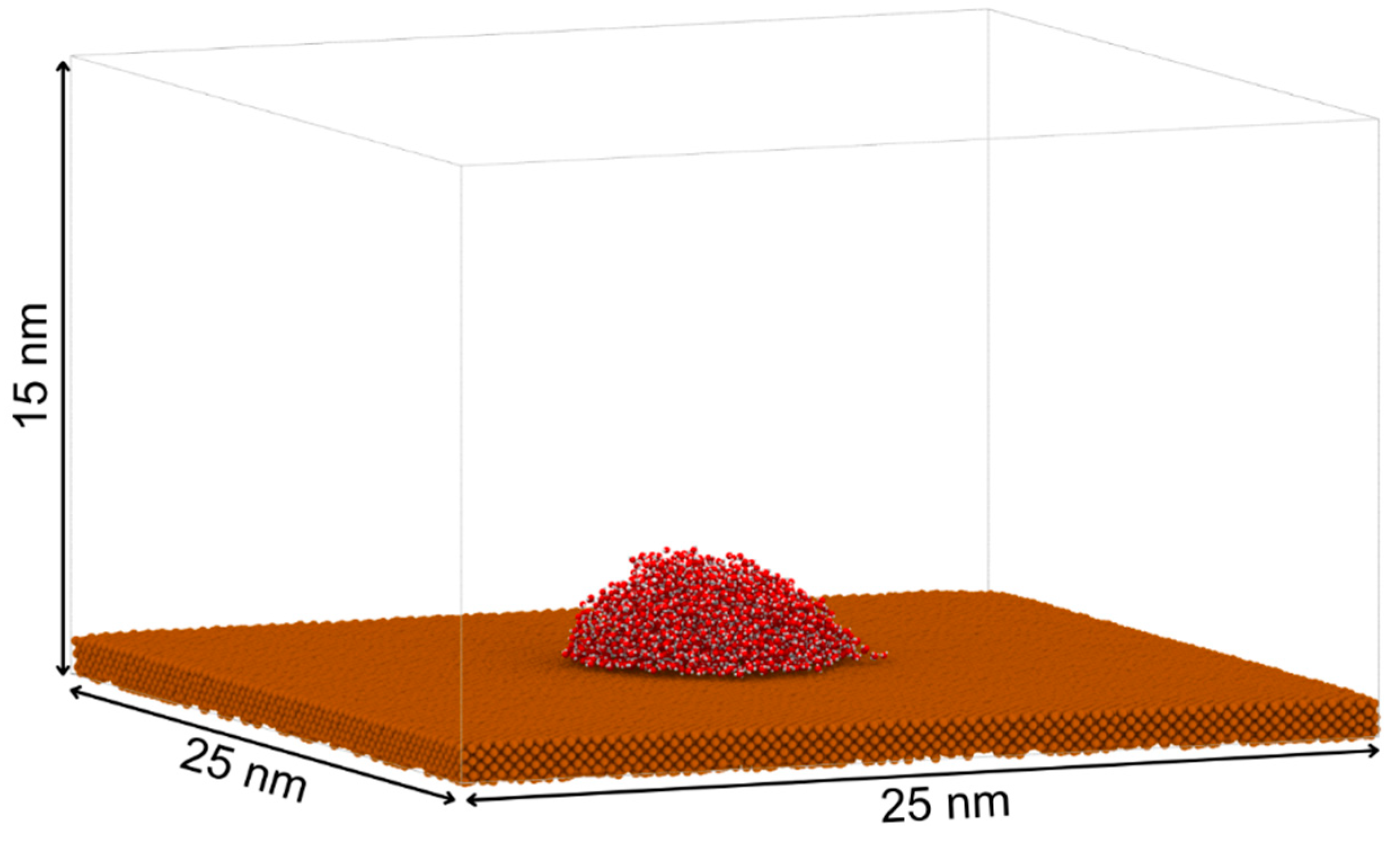
The copper substrate was generated using the open-source tool Atomsk [8], constructing a 10nm×10nm×1nm slab with an FCC (111) crystal structure and a lattice constant of 3.615 Å [9,10,11,12,13]. This thickness was sufficient to mimic a semi-infinite solid while minimizing computational cost. The (111) surface was chosen in accordance with prior copper–water wetting studies. The water phase consisted of a pre-equilibrated 5 nm×5 nm×5nm TIP4P/2005 water block. A vertical separation of 0.15 nm was maintained between the water block and copper surface to prevent atomic overlap during initialization [14]. Periodic boundary conditions were applied in the x, y, and z directions, with a simulation box height of 15 nm to avoid spurious interactions between periodic images along z.
Figure 1.
Equilibrated configuration of a 5 nm × 5 nm × 5 nm TIP4P/2005 water droplet placed on a 1 nm thick copper substrate (25 nm × 25 nm) within a simulation box of 15 nm height.
Figure 1.
Equilibrated configuration of a 5 nm × 5 nm × 5 nm TIP4P/2005 water droplet placed on a 1 nm thick copper substrate (25 nm × 25 nm) within a simulation box of 15 nm height.
Force Fields and Interactions
Water–water interactions were modeled using the special pair style implementation of TIP4P potential in LAMMPS [15]. Oxygen–oxygen LJ parameters were set to kcal/mol and , while hydrogen–hydrogen and oxygen–hydrogen LJ interactions were set to zero, as per the TIP4P/2005 specification. Long-range electrostatics were treated using the PPPM/tip4p solver [16] with an accuracy of 10−4. Bond lengths () and bond angles ) within water molecules were constrained using the SHAKE algorithm [17,18] with a tolerance of 10−4, ensuring minimal intramolecular distortion. Copper–copper interactions were described using the Modified Embedded Atom Method (MEAM) potential [19,20,21,22]. Cross-interactions between oxygen and copper were represented by an LJ potential with and a variable tuned during parameterization, while hydrogen–copper LJ terms were set to zero.
Simulation Protocol
Initial atomic velocities were assigned from a Maxwell–Boltzmann distribution at 300 K and rescaled to match the target temperature. Separate Nosé–Hoover thermostats (relaxation time 500 fs) were applied to water and copper atoms. To prevent rigid-body drift, atoms in the bottom most layer of the copper slab were restrained using a harmonic spring (). Each simulation consisted of a 500 ps equilibration run followed by a 500 ps production run, both using a 1 fs timestep. Atomic configurations were saved every 500 steps for post-processing and trajectory analysis.
Contact Angle Estimation Protocol
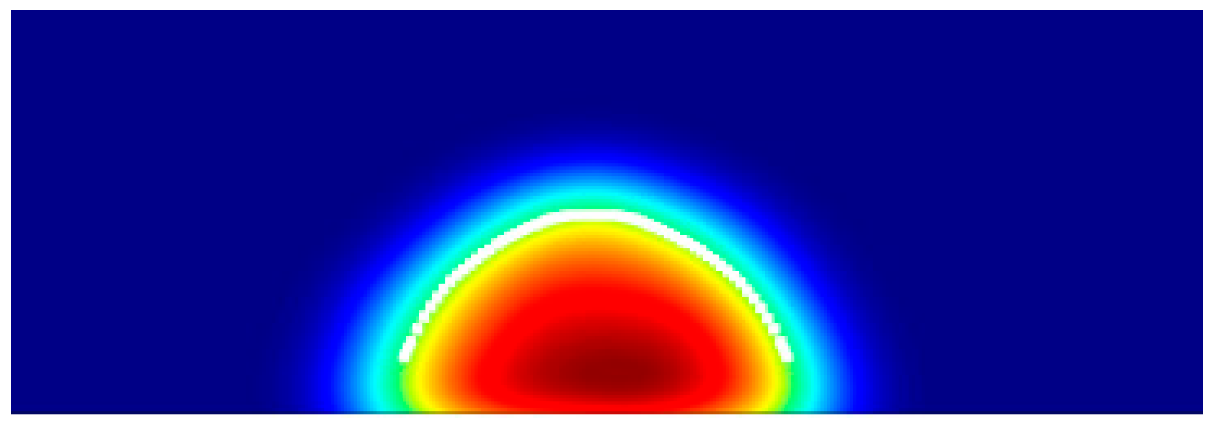
The contact angle was determined from the two-dimensional (2D) density profile of the liquid along the x–z plane. The profile was segmented into regions approaching the solid surface to identify the zone where the liquid density changes sharply, corresponding to the liquid–vapor interface. The spatial location of this interface was used to extract the droplet contour. A circle (or arc) was then fitted to the contour, and the contact angle was calculated from the angle between the tangent to the fitted curve at the solid–liquid intersection point and the horizontal surface line, following the method described in [23].
Step 1: Density Field Construction from Oxygen Atom Positions
A custom Python script was developed to perform 2D kernel density estimation (KDE) [24,25] on a frame-by-frame basis, using oxygen atom positions extracted from the molecular dynamics trajectory in XYZ format. For each frame, only oxygen atoms were selected, and their x and z coordinates were used for density calculation. The coordinates were interpolated onto a uniform grid with 1 Å spacing, and a Gaussian KDE (bandwidth = 0.4 Å) was applied to obtain a smooth, continuous density field from the discrete atomic positions. This procedure yielded a 2D density map for each frame, which was saved as an individual CSV file for subsequent analysis.
Step 2: Interface Extraction via Adaptive Density Thresholding
The csv files are then used to plot the density of water atoms over X-Z planes using MATLAB [26]. The script begins by loading all CSV files, each containing a two-dimensional density field sampled from a uniform grid with a spacing of 1 Å. For each frame, the density matrix is cropped to focus on the area of interest. To differentiate between liquid and vapor in the density map, a global threshold i.e., t=0.5 [27] is calculated dynamically using Bernsen’s Method[28] :
When the condition holds true, this produces a binary mask, where the pixel is classified as "liquid" and records X and Z axis points along the interface. This heuristic method automatically adapts to changes in overall density between frames, ensuring that the extraction of interfaces remains reliable even with varying droplets. A simple moving average is applied to smooth these points, yielding for robust fitting and noise reduction.
Figure 2.
Visualization of the liquid–vapor interface obtained by applying a density threshold (step 2) to a two-dimensional density map for the selected simulation frame, highlighting the phase boundary in the droplet profile.
Figure 2.
Visualization of the liquid–vapor interface obtained by applying a density threshold (step 2) to a two-dimensional density map for the selected simulation frame, highlighting the phase boundary in the droplet profile.
Step 3: Circle Fitting of the Liquid–Vapor Interface
An algebraic Least-Squares Circle Fitting[29] is performed on the smoothed points and to determine the best matches this smooth interface, by solving the linear system:
Linearizing by expanding each term and rearranging yields the linear system
This can be taken as whereas, So that the circle parameters follow as:
Figure 3.
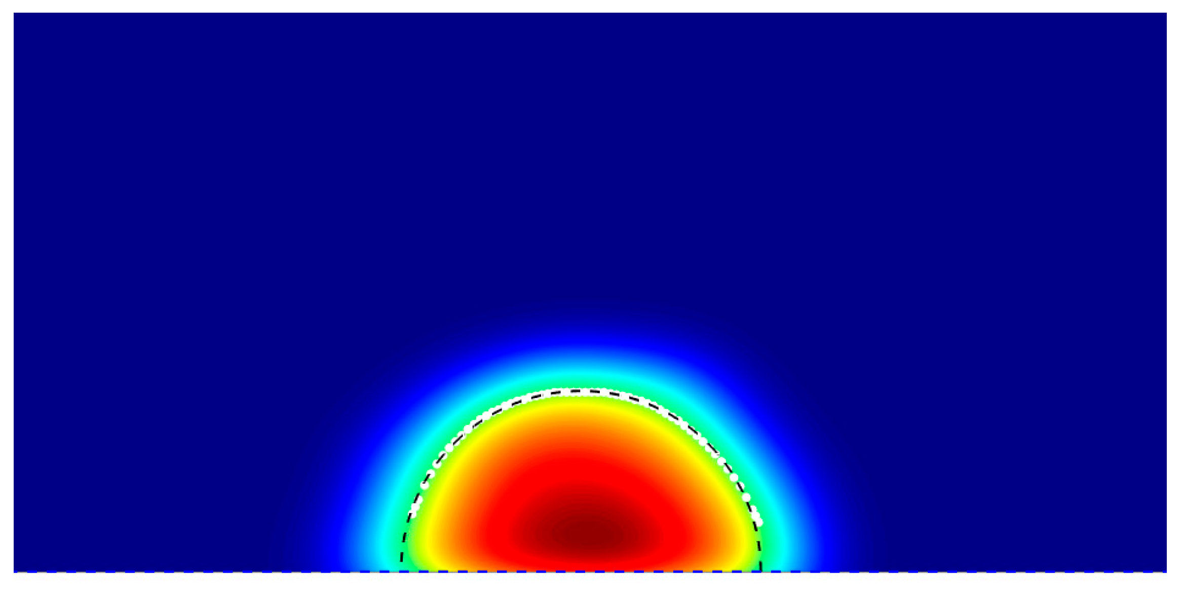
Two-dimensional density map of a droplet showing the liquid–vapor interface (black dashed line) extracted using a density threshold, enabling precise determination of the droplet’s contact angle.
Figure 3.
Two-dimensional density map of a droplet showing the liquid–vapor interface (black dashed line) extracted using a density threshold, enabling precise determination of the droplet’s contact angle.
Step 4: Accuracy Assessment of Circle Fit Using MSE
A Mean Squared Error[30] test is performed to determine the accuracy of circle fitting over the liquid-vapor interface. MSE is calculated by taking the average of the squared residuals, where the residual is the difference between the predicted value and the actual value for each data point in each frame. MSE is calculated by the following [31]:
A small MSE, specifically one that is lower than , indicates that the interface is accurately represented by a circle or arc[31].
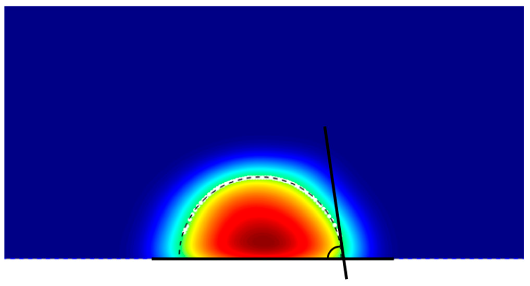
Step 5: Contact Angle Calculation from Fitted Geometry
Here, , signifying the number of frames, which can significantly aid in determining the contact angle. Scientifically, the script creates a horizontal reference line along the Z axis and a tangent line to the arc from the reference line and estimates the angle between these two lines using the expression:
Hence, the angle formed between these two lines is referred to as the contact angle of the solid-liquid interface. We use this method to estimate the contact angle for each frame and calculate the average along with the standard deviation of the contact angle.
Figure 4.
Determination of droplet contact angle from the two-dimensional density map by fitting a tangent line to the liquid–vapor interface (black dashed line) at the contact point with the surface.
Figure 4.
Determination of droplet contact angle from the two-dimensional density map by fitting a tangent line to the liquid–vapor interface (black dashed line) at the contact point with the surface.
In this study, the wetting behavior of copper surfaces was systematically investigated by varying the Lennard–Jones (LJ) interaction strength parameter () between the oxygen sites of TIP4P/2005 water molecules and copper atoms. The ε value was initially varied from 0.10 to 0.80 kcal/mol in increments of 0.05 kcal/mol to capture the overall hydrophilic–hydrophobic transition. As increased, the interaction between water and copper strengthened, resulting in greater droplet spreading and a pronounced reduction in the measured contact angle. This transition is clearly illustrated in Figure 5, which shows a steep decline in contact angle with increasing , shifting the surface behavior from hydrophobic to strongly hydrophilic.
To resolve finer changes in the hydrophilic regime, was further varied from 0.20 to 0.40 kcal/mol in smaller increments of 0.02 kcal/mol. The results, presented in Figure 6, reveal a consistent and monotonic decrease in contact angle with increasing . At lower values, droplets retained higher contact angles, indicative of limited wetting. As increased, enhanced attractive interactions between water oxygen atoms and copper atoms caused droplets to spread more extensively, reducing the contact angle to below at the highest tested values.
Overall, these results demonstrate a clear and tunable relationship between the LJ energy parameter ε and the wetting properties of copper surfaces. By adjusting , the simulated copper–water interface can be driven from a non-wetting state to complete wetting, offering precise control over interfacial behavior. This tunability provides a valuable framework for calibrating force field parameters to match experimental observations and for predicting wetting phenomena in nanoscale applications involving copper–water systems.
Validation to Experimental WCA:
To validate the force field parameterization, we performed a fine-grained sweep of the Lennard–Jones energy parameter () for the oxygen–copper interaction in the range 0.20-0.30 kcal/mol, using increments of 0.02 kcal/mol. This range was chosen to encompass experimentally reported water contact angles (WCA) for copper surfaces in air, which typically lie between 50.2° and 82.3°. The simulation results revealed a clear and monotonic trend: as increased, the attractive interaction between water and copper strengthened, promoting droplet spreading and reducing the contact angle. Simulated WCA values ranged from 83.48° at =0.20 kcal/mol to 37.83° at =0.30 kcal/mol. Within the narrower range of =0.20-0.28 kcal/mol, the predicted contact angles closely matched experimental values, with deviations well within a few degrees (Table 1).
This agreement underscores the accuracy of the chosen force field in reproducing macroscopic wetting behavior from atomistic simulations. Importantly, the close correspondence between simulation and experiment suggests that tuning ε can be an effective strategy for bridging the gap between molecular-scale modeling and real-world surface wettability measurements. By calibrating the interaction strength in this manner, our simulations can capture not only the qualitative hydrophilic–hydrophobic transition but also quantitatively match observed wetting characteristics of copper surfaces under ambient conditions. Overall, this validation provides strong evidence that the parameterized oxygen–copper interaction in our TIP4P/2005–Cu(111) model can accurately reproduce experimentally observed wetting behavior, thereby increasing confidence in its predictive capability for nanoscale interfacial studies.
3. Nanochannel Evaporation Studies
To investigate nanoscale evaporation mechanisms under confinement, we constructed a copper–water nanochannel system as shown schematically in Figure 7. The geometry was designed to emulate a liquid reservoir feeding a sequential series of narrow channels, which then transitioned into vapor collection regions. This allowed spatially resolved tracking of evaporation onset, propagation, and vapor transport.
The copper walls were modeled using the Modified Embedded Atom Method (MEAM) potential to capture many-body metallic bonding effects and realistic elastic response. Water molecules were represented by the TIP4P/2005 model, chosen for its high fidelity in reproducing thermophysical properties and hydrogen-bond structure. Long-range electrostatics were treated using the PPPM/tip4p solver with a target accuracy of 10-4, ensuring accurate handling of Coulomb interactions. The water–copper cross-interaction was described via a Lennard–Jones potential with parameters ( kcal/mol, Å), consistent with our wetting calibration studies, ensuring that adhesion strength reflected experimentally observed hydrophilic behavior of copper.
3.1. Materials and Methods for Nanochannel Evaporation
The simulation box dimensions were 4.25nm×3.2535nm×25nm in x, y, and z. The dimension along x-axis (4.25nm) is chosen to resemble a 2nm channel width with 1nm copper plate on either side. Precise modeling of the copper into 1nm is difficult while respecting the lattice structure face centered cubic (fcc) 111. Hence, an additional 0.25 nm will appear in the x-axis, making a total of 4.25nm. In the y-axis, at least 3 times of cutoff radius (0.85nm) is minimum preferred to avoid periodic image interaction artifacts. Due to this, we chose a value greater than 3 nm, which turned out to be 3.2535 nm to keep the lattice structure arrangement without gaps across the periodic boundary conditions (PBC). Periodic boundary conditions were applied along all directions. The channel interior was subdivided into physically distinct regions: Reservoir (liquid inlet), Seven sequential channel sections (Channel 1–7), Five vapor regions (Vapor 1–5), and Cooling region downstream. Each region’s spatial extent in the z-direction is labeled in Figure 7. The geometry ensured a controlled progression from liquid-dominated flow near the inlet to vapor-dominated flow near the outlet, enabling temperature-dependent mapping of evaporation behavior. Water molecules were initially positioned as a pre-equilibrated block, with a small gap away from the copper walls to prevent atom overlap. Copper atoms were tethered via a weak spring with respect to their initial positions to prevent rigid body drift, and SHAKE constraints were applied to water molecules to preserve TIP4P/2005 geometry.
Thermal control was implemented using region-specific Langevin thermostats: Reservoir and inlet channels (1–3) maintained at 300 K to supply stable liquid. Mid-channel and vapor regions (4–7, Vapor 1–5) thermostated to target evaporation temperatures of 300, 350, 400, 450, 500, 525, 550 and 600 K depending on the case. Cooling section maintained at 300 K to mimic heat removal. 1 fs integration timestep was used. The simulation length was 250,000 steps (250 ps), sufficient to capture both transient and quasi-steady evaporation stages.
Dynamic groups tracked water molecules in each spatial region every 10 steps. Key metrics included: Number of molecules per region, Copper and water temperatures, Potential and total energies, Evaporation curves smoothed with a moving-average filter considering 50 values. MATLAB post-processing generated temporal depletion and accumulation plots (Figures 9 and 10), highlighting the migration of water molecules from liquid-filled channels into vapor regions.
3.2. Results and Discussion
Figure 7 presents a schematic of the molecular dynamics simulation setup. The copper walls (brown) confine the water phase (oxygen in red, hydrogen in white), with spatial segmentation into reservoir, channels, and vapor regions. The color-coded segmentation (blue for cooler inlet sections, red for heated mid-to-outlet sections) facilitates independent temperature control, simulating localized heating scenarios as found in micro-evaporators and nuclear microchannel heat exchangers. Figure 8 provides representative snapshots of water confined in the nanochannel for system temperatures of 300 K, 400 K, 500 K, and 600 K. At 300 K, the liquid column remains intact, with minimal vapor-phase molecules above the interface. By 400 K, localized evaporation becomes visible near the heated sections, with the vapor front expanding downstream. At 500 K, the vapor phase occupies a substantial portion of the channel’s upper regions, and at 600 K, rapid boiling-like behavior is observed, with dispersed vapor molecules filling the downstream vapor regions. The qualitative transition from surface-layer evaporation to bulk-phase vaporization is evident.
Figure 9 shows the temporal evolution of the number of water molecules in Channels 2–7 for temperatures from 300 K to 600 K. At 300 K, curves remain nearly flat, indicating negligible evaporation. At 400–500 K, gradual depletion is seen in heated channels (4–7), with the slope increasing with temperature. At 600 K, liquid in downstream channels depletes rapidly within ~100 ps, indicating a high evaporation rate and strong mass flux toward vapor regions. These trends reflect the balance between latent heat requirements and interfacial adhesion forces. Strong copper–water interactions delay the onset of net evaporation by stabilizing the interfacial water layer, but once thermal energy exceeds this adhesion threshold, mass loss accelerates sharply.
Figure 10 illustrates the complementary growth of vapor content in regions 1–5. At 300 K, vapor regions remain largely unoccupied. At 400–500 K, vapor regions closest to the heated channels fill gradually, while distant vapor zones remain sparse, indicating a diffusion-limited transport regime. At 600 K, all vapor regions fill rapidly, with the highest occupancy in regions adjacent to heated channels. Panel Figure 10(f) summarizes the steady-state water content per region, averaged over the final 50 frames. This aggregation shows a clear inverse correlation between channel liquid content and vapor occupancy, reinforcing the view that localized heating not only drives phase change but also redistributes fluid mass along the channel’s axial direction.
The observed temperature-dependent evaporation rates can be explained by competition between cohesive hydrogen-bond networks within TIP4P/2005 water and adhesive interactions with the copper wall. At low T, cohesive forces dominate, maintaining molecular layering near the wall and suppressing vapor formation. As T rises, thermal agitation disrupts hydrogen bonding and overcomes adhesion, enabling rapid molecular escape into the vapor phase. The spatial segmentation of the channel further reveals that evaporation onset is not uniform. In moderately heated cases (400–500 K), evaporation initiates downstream of the initial contact with heated walls, suggesting a finite thermal penetration depth before sufficient molecular excitation occurs. In highly heated cases (600 K), the entire heated section contributes to vapor generation, consistent with a boiling-like transition where bulk kinetic energy exceeds cohesive energy.
4. Conclusion
We created and tested a copper–water interaction model for TIP4P/2005 water on a Cu(111) surface, adjusting the oxygen–copper Lennard–Jones energy parameter so that the simulated water contact angles matched experimental values. The validated model showed that increasing ε lowers the contact angle, allowing precise control of surface wetting from water-repelling (hydrophobic) to water-attracting (hydrophilic). When we used this model in nanochannel evaporation simulations, we found that evaporation strongly depends on temperature: at low temperatures, strong water–copper attraction and hydrogen bonding keep water from evaporating, but at higher temperatures, evaporation becomes rapid and can resemble boiling. Dividing the channel into different regions revealed that evaporation does not start everywhere at once, but mainly in heated areas. This study provides a dependable force-field model for simulating copper–water interactions and a detailed framework for understanding and controlling nanoscale evaporation in metallic channels. The results are useful for designing advanced cooling systems such as microreactors, micro-evaporators, and compact heat exchangers, and they also provide high-quality data for larger-scale models and machine learning tools.
Data Availability:
All input scripts, LAMMPS data files, and post-processing tools used in this study will be made available upon reasonable request.
Author Contributions
Conceptualization, S.Y.; Methodology, S.Y. and M.M.; Software, S.Y.; Validation, S.Y., M.M., and J.M.; Formal Analysis, S.Y., M.M., J.M., and M.T.; Investigation, S.Y.; Resources, S.Y.; Data Curation, S.Y.; Writing – Original Draft Preparation, S.Y.; Writing – Review & Editing, S.Y., M.M., J.M., and M.T.; Visualization, S.Y., Supervision, S.Y.; Project Administration, S.Y.; Funding Acquisition, S.Y.
Acknowledgments
The authors acknowledge computational resources provided by University of New Haven and support from award 31310023M0029 from Acquisition Management Division, Nuclear Regulatory Commission (NRC). The statements, findings, conclusions, and recommendations are those of the authors and do not necessarily reflect the view of the Acquisition Management Division or the US Nuclear Regulatory Commission.
Conflicts of Interest
The authors declare no conflict of interest.
References
- Stewart, C.L.; Goldblum, B.L.; Abbott, R.G.; Appleby, L.; Borghetti, B.J.; Hollingshead, V.; Whetzel, J.H. Machine Learning for Reactor Power Monitoring with Limited Labeled Data. Nuclear Instruments and Methods in Physics Research Section A: Accelerators, Spectrometers, Detectors and Associated Equipment 2025, 1073, 170285. [Google Scholar] [CrossRef]
- Sahin, E. Machine Learning-Driven Uncertainty Quantification and Parameter Analysis in Fire Risk Assessment for Nuclear Power Plants. 2025.
- Ramezani, I.; Moshkbar-Bakhshayesh, K.; Vosoughi, N.; Ghofrani, M.B. Applications of Soft Computing in Nuclear Power Plants: A Review. Progress in Nuclear Energy 2022, 149, 104253. [Google Scholar] [CrossRef]
- Lafleur, B. Development and Assessment of Machine Learning Techniques for Non-Intrusive Probabilistic Surrogate Modeling of High-Fidelity Nuclear Reactor Simulations. PhD Thesis, 2023.
- Huang, H.; Lu, D.; Liu, Y.; Sui, D.; Xie, F.; Ding, H. Research on a Rapid Prediction Method for Multi-Physics Coupled Fields in Small Lead-Cooled Fast Reactors Based on Machine Learning. Nuclear Engineering and Design 2025, 438, 114065. [Google Scholar] [CrossRef]
- Hu, G.; Prasianakis, N.; Churakov, S.V.; Pfingsten, W. Performance Analysis of Data-Driven and Physics-Informed Machine Learning Methods for Thermal-Hydraulic Processes in Full-Scale Emplacement Experiment. Applied Thermal Engineering 2024, 245, 122836. [Google Scholar] [CrossRef]
- Abascal, J.L.; Vega, C. A General Purpose Model for the Condensed Phases of Water: TIP4P/2005. The Journal of chemical physics 2005, 123. [Google Scholar] [CrossRef]
- Hirel, P. Atomsk: A Tool for Manipulating and Converting Atomic Data Files. Computer Physics Communications 2015, 197, 212–219. [Google Scholar] [CrossRef]
- Straumanis, M.E.; Yu, L.S. Lattice Parameters, Densities, Expansion Coefficients and Perfection of Structure of Cu and of Cu–In α Phase. Foundations of Crystallography 1969, 25, 676–682. [Google Scholar] [CrossRef]
- Sinha, S.K. Lattice Dynamics of Copper. Phys. Rev. 1966, 143, 422–433. [Google Scholar] [CrossRef]
- Jona, F.; Marcus, P.M. Structural Properties of Copper. Phys. Rev. B 2001, 63, 094113. [Google Scholar] [CrossRef]
- Davis, H.L.; Faulkner, J.S.; Joy, H.W. Calculation of the Band Structure for Copper as a Function of Lattice Spacing. Phys. Rev. 1968, 167, 601–607. [Google Scholar] [CrossRef]
- Davey, W.P. Precision Measurements of the Lattice Constants of Twelve Common Metals. Phys. Rev. 1925, 25, 753–761. [Google Scholar] [CrossRef]
- YD, S.; Maroo, S.C. Origin of Surface-Driven Passive Liquid Flows. Langmuir 2016. [Google Scholar] [CrossRef] [PubMed]
- Thompson, A.P.; Aktulga, H.M.; Berger, R.; Bolintineanu, D.S.; Brown, W.M.; Crozier, P.S.; In’t Veld, P.J.; Kohlmeyer, A.; Moore, S.G.; Nguyen, T.D. LAMMPS-a Flexible Simulation Tool for Particle-Based Materials Modeling at the Atomic, Meso, and Continuum Scales. Computer physics communications 2022, 271, 108171. [Google Scholar] [CrossRef]
- Abascal, J.L.; Vega, C. A General Purpose Model for the Condensed Phases of Water: TIP4P/2005. The Journal of chemical physics 2005, 123. [Google Scholar] [CrossRef]
- Hammonds, K.D.; Ryckaert, J.-P. On the Convergence of the SHAKE Algorithm. Computer physics communications 1991, 62, 336–351. [Google Scholar] [CrossRef]
- Andersen, H.C. Rattle: A “Velocity” Version of the Shake Algorithm for Molecular Dynamics Calculations. Journal of computational Physics 1983, 52, 24–34. [Google Scholar] [CrossRef]
- Lee, B.-J.; Ko, W.-S.; Kim, H.-K.; Kim, E.-H. The Modified Embedded-Atom Method Interatomic Potentials and Recent Progress in Atomistic Simulations. Calphad 2010, 34, 510–522. [Google Scholar] [CrossRef]
- Lee, B.-J.; Baskes, M.I. Second Nearest-Neighbor Modified Embedded-Atom-Method Potential. Phys. Rev. B 2000, 62, 8564–8567. [Google Scholar] [CrossRef]
- Baskes, M.I. Determination of Modified Embedded Atom Method Parameters for Nickel. Materials Chemistry and Physics 1997, 50, 152–158. [Google Scholar] [CrossRef]
- Baskes, M.I. Modified Embedded-Atom Potentials for Cubic Materials and Impurities. Phys. Rev. B 1992, 46, 2727–2742. [Google Scholar] [CrossRef]
- Shi, B.; Dhir, V.K. Molecular Dynamics Simulation of the Contact Angle of Liquids on Solid Surfaces. The Journal of chemical physics 2009, 130. [Google Scholar] [CrossRef]
- Węglarczyk, S. Kernel Density Estimation and Its Application. In Proceedings of the ITM web of conferences; EDP Sciences, 2018; Vol. 23; p. 00037. [Google Scholar]
- Chen, Y.-C. A Tutorial on Kernel Density Estimation and Recent Advances. Biostatistics & Epidemiology 2017, 1, 161–187. [Google Scholar] [CrossRef]
- Elhorst, J.P. Matlab Software for Spatial Panels. International Regional Science Review 2014, 37, 389–405. [Google Scholar] [CrossRef]
- Chen, Y.-C. Molecular Dynamics Study Of Phase Change And Interfacial Behavior In Nanoconfined Argon. 2025.
- Eyupoglu, C. Implementation of Bernsen’s Locally Adaptive Binarization Method for Gray Scale Images. The Online Journal of Science and Technology 2017, 7, 68–72. [Google Scholar]
- Chernov, N.; Lesort, C. Least Squares Fitting of Circles. J Math Imaging Vis 2005, 23, 239–252. [Google Scholar] [CrossRef]
- Bickel, P.J.; Doksum, K.A. Mathematical Statistics: Basic Ideas and Selected Topics, Volumes I-II Package; Chapman and Hall/CRC, 2015. [Google Scholar]
- James, G.; Witten, D.; Hastie, T.; Tibshirani, R. An Introduction to Statistical Learning; Springer Texts in Statistics; Springer New York: New York, NY, 2013; ISBN 978-1-4614-7137-0. [Google Scholar]
Figure 5.
Measured water contact angle on a copper surface as a function of interaction energy (). The results show a sharp decrease in contact angle with increasing , indicating a transition from hydrophobic to highly hydrophilic behavior at higher interaction strengths.
Figure 5.
Measured water contact angle on a copper surface as a function of interaction energy (). The results show a sharp decrease in contact angle with increasing , indicating a transition from hydrophobic to highly hydrophilic behavior at higher interaction strengths.
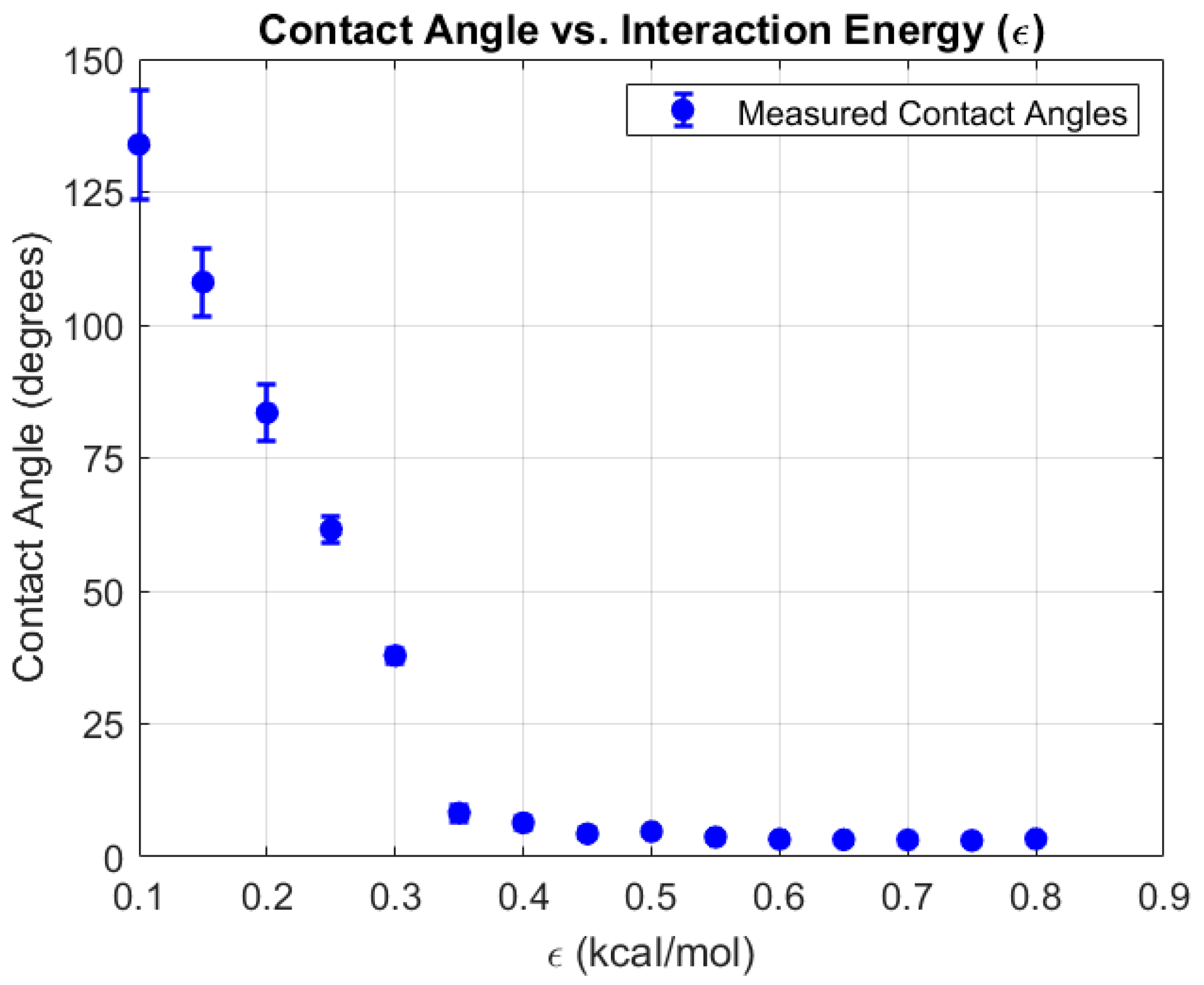
Figure 6.
Variation of water contact angle on a copper surface as a function of interaction energy (ε) obtained from molecular dynamics simulations. Higher interaction energies result in stronger wetting behavior, as indicated by the decreasing contact angle.
Figure 6.
Variation of water contact angle on a copper surface as a function of interaction energy (ε) obtained from molecular dynamics simulations. Higher interaction energies result in stronger wetting behavior, as indicated by the decreasing contact angle.
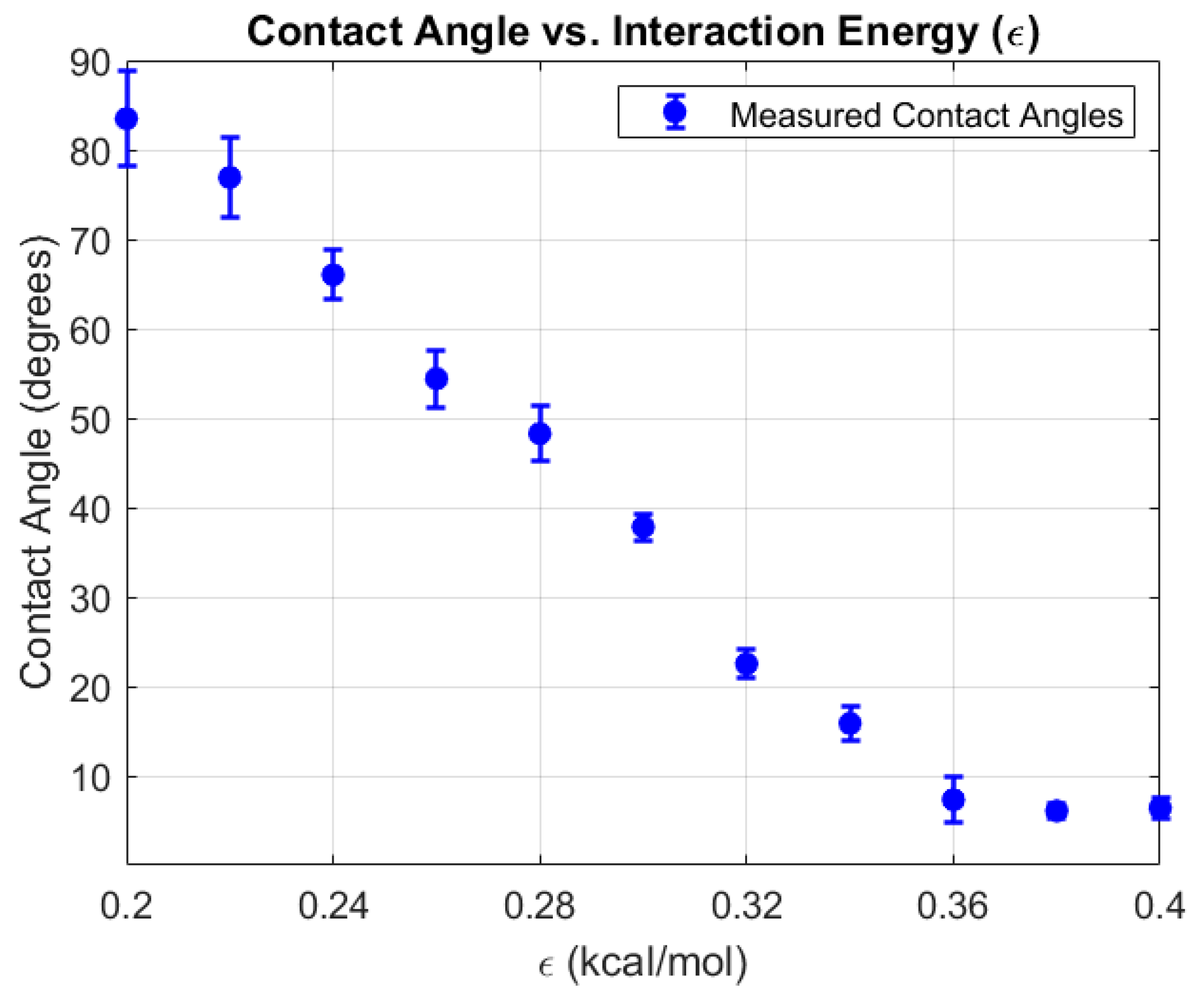
Figure 7.
Schematic representation of the molecular dynamics simulation setup for water confined in a copper nanochannel using the TIP4P/2005 water model. The system consists of a 2 nm reservoir, seven sequential channel sections (blue: channels 1–3; red: channels 4–7), and five vapor regions, followed by a cooling region. The copper walls are shown in brown, and water molecules in red/white. The spatial divisions (in nm) indicate the lengths of each region used for analysis of transport and phase behavior.
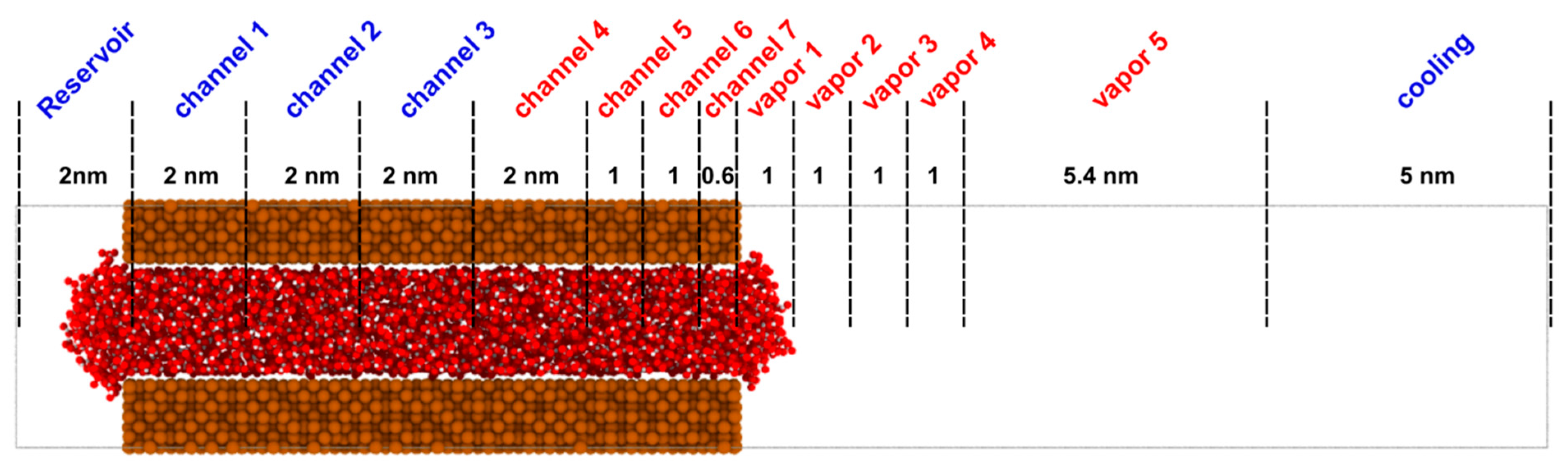
Figure 8.
Snapshots of molecular dynamics simulations showing water confined in a copper nanochannel at temperatures ranging from 300 K to 600 K. As the temperature increases, the extent of evaporation and vapor-phase water molecules (red) above the liquid column becomes more pronounced.
Figure 8.
Snapshots of molecular dynamics simulations showing water confined in a copper nanochannel at temperatures ranging from 300 K to 600 K. As the temperature increases, the extent of evaporation and vapor-phase water molecules (red) above the liquid column becomes more pronounced.
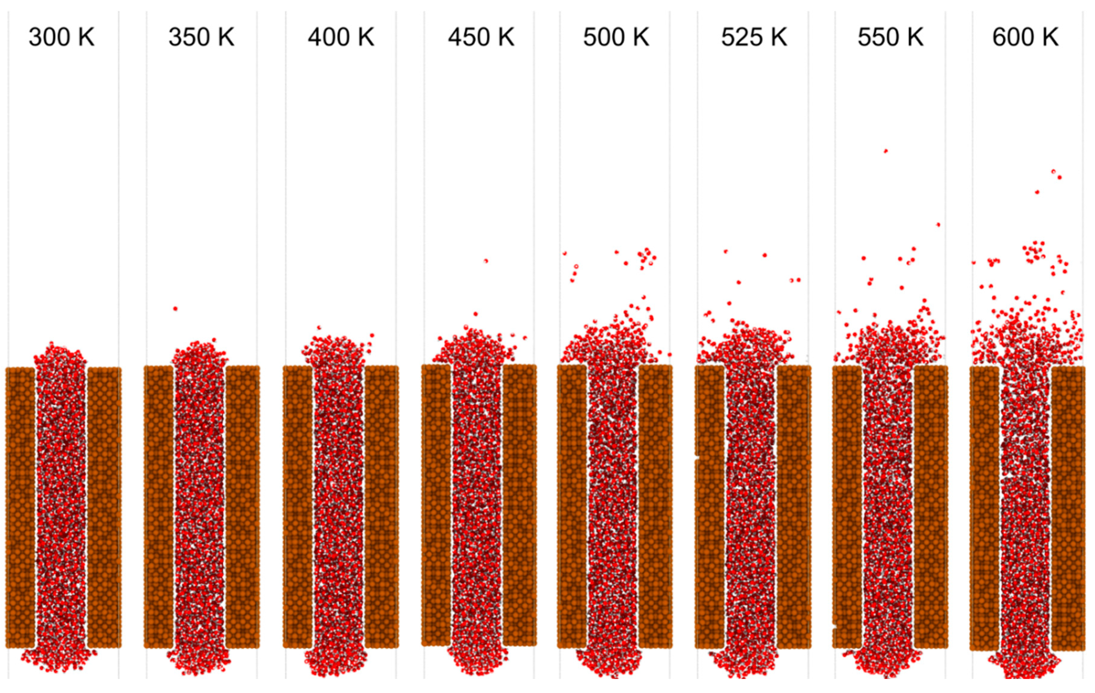
Figure 9.
Temporal variation of the number of water molecules in channels 2–7 for different system temperatures (300–600 K). Data are smoothed using a moving average window to highlight overall trends. Panels (a)–(f) correspond to Channels 2–7, respectively, with each curve representing a different temperature as indicated in the shared legend.
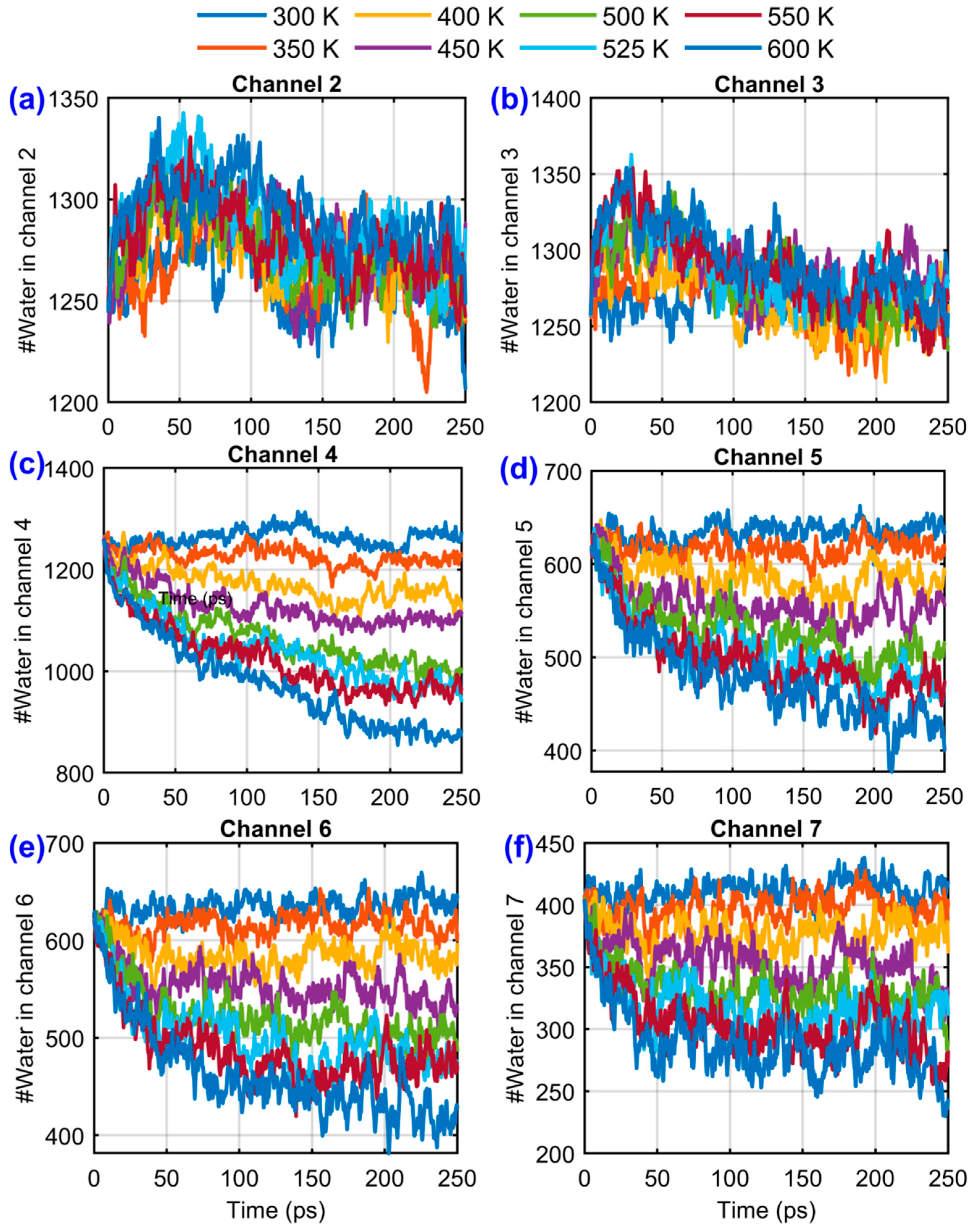
Figure 10.
Temporal evolution of the number of water molecules in vapor regions 1–5 at different system temperatures (300–600 K), panels (a)–(e). Data are smoothed using a moving-average filter to highlight overall trends. Panel (f) summarizes the final water content in each channel and vapor region, calculated as the average over the last 50 simulation frames for each temperature.
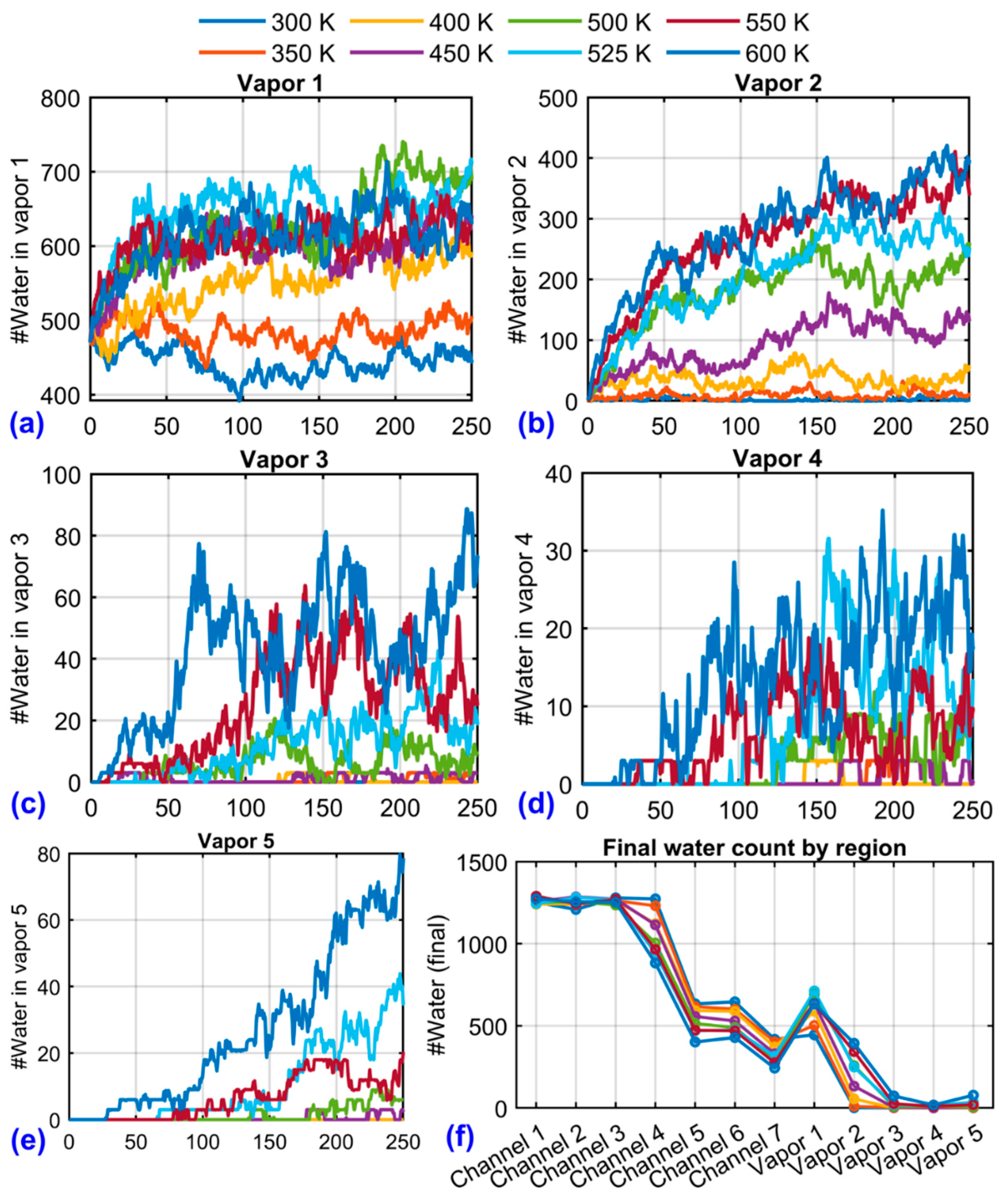

Table 1.
Represents the Validation of estimated contact angle with experimental WCA of copper.
| Eps (kcal/mol) | Contact Angle (°) | Std. Dev. (°) | Experimental WCA (°) |
| 0.2 | 83.48 | 5.28 | 82.3 |
| 0.22 | 76.91 | 4.51 | |
| 0.24 | 66.01 | 2.72 | |
| 0.26 | 54.42 | 3.2 | 50.2 |
| 0.28 | 48.27 | 3.11 |
Disclaimer/Publisher’s Note: The statements, opinions and data contained in all publications are solely those of the individual author(s) and contributor(s) and not of MDPI and/or the editor(s). MDPI and/or the editor(s) disclaim responsibility for any injury to people or property resulting from any ideas, methods, instructions or products referred to in the content. |
© 2025 by the authors. Licensee MDPI, Basel, Switzerland. This article is an open access article distributed under the terms and conditions of the Creative Commons Attribution (CC BY) license (http://creativecommons.org/licenses/by/4.0/).
Copyright: This open access article is published under a Creative Commons CC BY 4.0 license, which permit the free download, distribution, and reuse, provided that the author and preprint are cited in any reuse.


