Reply To: Re-Evaluating Local Genetic Correlation Analysis in the HDL Framework

Yuying Li; Yudi Pawitan; Xia Shen

doi:10.20944/preprints202508.1096.v1

Submitted:

08 August 2025

Posted:

14 August 2025

You are already at the latest version

Abstract

The LAVA method has been proposed for detecting local genetic correlations between traits. We show, using theoretical analysis and simulations, that LAVA’s “fixed-effects” model does not estimate genetic correlation in the statistical genetics sense, but instead detects the presence of regional genetic effects. This mis-specification leads to inflated type-I error under the null, particularly when causal variants are sparse, and can produce apparent “correlations” arising solely from unshared, trait-specific signals. In contrast, the random-effects model implemented in HDL-L correctly targets variant-level genetic correlation and remains well-calibrated. Our results indicate that LAVA findings may be widely misinterpreted, and we recommend caution and the use of random-effects–based approaches such as HDL-L for valid inference.

Keywords:

genetic correlation

;

HDL-L

;

LAVA

;

apparent correlation

;

false positive

Subject:

Biology and Life Sciences - Other

We thank de Leeuw et al.[1] for their interest in our work and their clarification of the modeling assumptions underlying LAVA[2] (based on what they call the “fixed-effects” model) in contrast to HDL-L[3] (based on the random-effects model) for genetic correlation analysis. Unfortunately, we believe that there are some flaws in the statistical and biological basis of the LAVA model. Here, we offer the rationale for our modeling framework, highlighting why the random-effects model is statistically more appropriate and biologically more interpretable than the fixed-effects model for genetic effects modeling. Second, we demonstrate the reason why LAVA’s “fixed-effects” model does not reflect the underlying shared genetic architecture between two traits. Finally, we describe how LAVA detects statistical artifacts under null genetic correlation.

Regarding the second issue that de Leeuw et al. pointed out in our previous simulation on the use of different LD references, we agree that this may have introduced additional sources of bias. We used the 1000 Genomes reference data for LAVA because it was the only reference data provided for LAVA at the time. Nevertheless, in their Figure 1, de Leeuw et al. have now shown that the problem of false positives when using LAVA for the random-effects model remains even when the LD reference is corrected. Therefore, here we will focus on the issue of the underlying models. As they suggested, the problem of bias from using an LD reference from a different cohort requires further investigation.

Why the Random-Effects Model Is More Natural

In the random-effects model for a bivariate phenotype, a causal variant j’s effect

α_{j} \equiv (α_{1 j}, α_{2 j})

is assumed to vary randomly across the genome according to

α_{j} \sim N (0, [\begin{matrix} σ_{1}^{2} & r_{g} σ_{1} σ_{2} \\ r_{g} σ_{1} σ_{2} & σ_{2}^{2} \end{matrix}]),

where

σ_{1}^{2}

and

σ_{2}^{2}

are the genetic variance components, and

r_{g}

is the genetic correlation. In this formulation, heritability and genetic correlation are simple and transparent parameters of an underlying distribution, not statistics from an unspecified collection of unknown numbers. This modeling approach is natural for polygenic traits and standard in statistical genetics[4]. The LD Score Regression (LDSC)[5,6] method framework also assumes the same random-effects model when estimating genome-wide heritability and genetic correlation.

We shall discuss the statistical differences between the models below, but first, it is appropriate to explain the differences in terms of de Leeuw et al.’s simulation, as it explains how the data could have arisen and hence how natural the models are. In the random-effects model (coded in generate.rfx on LAVA’s GitHub page), effect sizes for each phenotype are sampled from the bivariate normal distribution above according to a specified heritability and genetic correlation. The genetic components are then computed as

G_{1} = X α_{1}, G_{2} = X α_{2},

where

X

is the genotype matrix, and

α_{1}

and

α_{2}

are the vectors of variants effects for each phenotype. So, each phenotype has its own causal variants and effect sizes, and the genetic components reflect the structure of their respective traits. This model is simple, interpretable, and matches the way phenotypes arise from their genotype.

In the fixed-effects model (coded in generate.ffx), the genetic components

G_{1}

and

G_{2}

are first generated in a similar way as in the random-effects model, but then

G_{2}

is modified as follows. (i) For

r_{g} = 0

, two independent candidates for

G_{2}

are generated; call this

G_{2 (1)}

and

G_{2 (2)}

. Then,

G_{2}

is computed as

G_{2} = w \cdot G_{2 (1)} + G_{2 (2)},

using the weight

w \equiv - G_{2 (2)}^{⊤} G_{1} / G_{2 (1)}^{⊤} G_{1},

so that

G_{2}

have an exact zero correlation with

G_{1}

. (ii) For

r_{g} \neq 0

, a candidate

G_{2}

is regressed on

G_{1}

, and the residual

R

is combined with

G_{1}

in order to achieve the target correlation:

G_{2} = r_{g} \cdot G_{1} + \sqrt{1 - r_{g}^{2}} \cdot R .

(The vectors

G_{1}

and

G_{2}

are scaled to have the specified heritabilities exactly; this does not change their correlation.)

Notwithstanding the name `fixed’ effects,

G_{1}

and

G_{2}

are actually computed using normal random genetic effects, not arbitrary fixed constants. In fact,

G_{1}

is exactly the same as in the random-effects model. The distinctive element is apparent in the construction of

G_{2}

, which now depends on the realized

G_{1}

. The steps guarantee a desired subject-level correlation between

G_{1}

and

G_{2}

, but the resulting

G_{2}

is no longer determined by its causal variants. In other words,

G_{2}

has no meaningful independent biological model, as it is defined in relation to

G_{1}

. This represents a significant departure from how we understand multivariate complex traits, where we still attribute each trait its own causal structure. Such `fixed-effects’ construction will become conceptually more complicated and biologically less meaningful if we consider more than two traits.

Thus, we argue that the random-effects model offers a more natural and interpretable foundation for evaluating local genetic correlation. It respects the biological assumption that each trait has its own causal basis and allows the correlation to arise from genuine shared genetic effects.

Discrepancy Between Subject-Level and Variant-Level Realized Genetic Correlations

Following the LAVA fixed-effects model, suppose we have a genotype matrix

X \in R^{N \times M}

, and two genetic effect vectors

α_{1}, α_{2} \in R^{M}

, generating genetic components:

G_{1} = X α_{1}

and

G_{2} = X α_{2} .

We perform a linear regression of

G_{2}

on

G_{1}

, and define the residual:

R = G_{2} - \hat{β} G_{1}, where \hat{β} = 〈 G_{1}, G_{2} 〉 / {∥ G_{1} ∥}^{2} .

Then we define a modified genetic component with target correlation

r_{g}

:

G_{2}^{alt} : = r_{g} \cdot G_{1} + \sqrt{1 - r_{g}^{2}} \cdot R .

By construction,

R ⊥ G_{1}

, so we obtain:

cor (G_{1}, G_{2}^{alt}) = r_{g} .

Suppose that

G_{2}^{alt} \in col (X)

, i.e., there exists a vector

α_{2}^{alt}

such that:

G_{2}^{alt} = X α_{2}^{alt} .

Then, since

G_{1} = X α_{1}

and

R = X δ

for some

δ \in R^{M}

, it follows that:

G_{2}^{alt} = X (r_{g} \cdot α_{1} + \sqrt{1 - r_{g}^{2}} \cdot δ) \Rightarrow α_{2}^{alt} = r_{g} \cdot α_{1} + \sqrt{1 - r_{g}^{2}} \cdot δ .

The correlation between

α_{1}

and

α_{2}^{alt}

is:

cor (α_{1}, α_{2}^{alt}) = \frac{r_{g} \cdot {∥ α_{1} ∥}^{2} + \sqrt{1 - r_{g}^{2}} \cdot 〈 α_{1}, δ 〉}{∥ α_{1} ∥ \cdot ∥ α_{2}^{alt} ∥} .

Hence, unless

〈 α_{1}, δ 〉 = 0

and

∥ α_{2}^{alt} ∥ = ∥ α_{1} ∥

, we do not obtain

cor (α_{1}, α_{2}^{alt}) = r_{g}

. In practice, the vector

δ

is not orthogonal to

α_{1}

, because it is induced by residualizing

G_{2}

with respect to

G_{1}

in phenotype space, not in genetic effect space. This means that forcing

cor (G_{1}, G_{2}^{alt})

to be an exact value would not remove the randomness in the realized

cor (α_{1}, α_{2}^{alt})

. Therefore, the so-called “fixed-effects model” is not a proper statistical genetics model, but rather a procedure for dealing with a special case of realized data. Below, we conduct a simulation to further demonstrate this point.

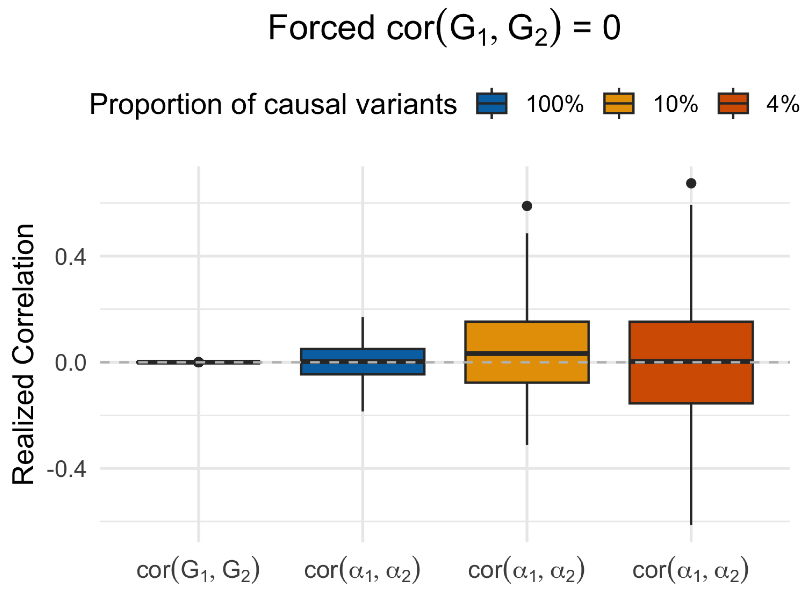
Based on the UK Biobank genotype data on the first region of chromosome 22, where we have

M = 185

genotyped variants, we randomly selected

N_{1} = 10, 000

and

N_{2} = 10, 000

individuals, standardized the

X \in R^{(N_{1} + N_{2}) \times M}

matrix column-wise to have mean 0 and variance 1. We then split the matrix into two independent subcohorts,

X_{1} \in R^{N_{1} \times M}

and

X_{2} \in R^{N_{2} \times M}

, corresponding to cohorts 1 and 2 respectively. Two independent genetic effect vectors

α_{1} \sim N (0, σ_{1}^{2} I_{M})

and

α_{2} \sim N (0, σ_{2}^{2} I_{M})

(where

σ_{1}

and

σ_{2}

were set to 1 and 2 respectively) were drawn to construct the genetic components:

G_{1} = X α_{1}

and

G_{2} = X α_{2} .

We then regressed

G_{2}

on

G_{1}

and extracted the residual vector:

R = G_{2} - \hat{β} G_{1}, where \hat{β} = G_{1}^{⊤} G_{2} / G_{1}^{⊤} G_{1} .

To force a desired subject-level genetic correlation of zero between

G_{1}

and a new genetic component

G_{2}^{alt}

, we constructed:

G_{2}^{alt} = r_{g} \cdot {\tilde{G}}_{1} + \sqrt{1 - r_{g}^{2}} \cdot \tilde{R},

where both

{\tilde{G}}_{1}

and

\tilde{R}

were standardized to have zero mean and unit variance. Next, we used the observed individuals in cohort 2 to compute

α_{2}^{alt}

by regressing the corresponding entries of

G_{2}^{alt}

on

X_{2}

via least squares:

α_{2}^{alt} = {(X_{2}^{⊤} X_{2})}^{- 1} X_{2}^{⊤} G_{2}^{alt} |_{cohort 2} .

We repeated this procedure over 100 simulations, each time recording: (i) the subject-level correlation

cor (G_{1}, G_{2}^{alt})

; (ii) the variant-level correlation

cor (α_{1}, α_{2}^{alt})

. The simulation procedure was repeated for 10% and 4% of M causal variants randomly selected from the region.

Despite enforcing

cor (G_{1}, G_{2}^{alt}) = r_{g}

, we observed that

cor (α_{1}, α_{2}^{alt})

was highly variable across simulations (Figure 1R). Note that as the proportion of causal variants decreased, the apparent correlation at variant-level, i.e.,

cor (α_{1}, α_{2})

increased in magnitude. This discrepancy confirms that the forced subject-level genetic correlation does not imply variant-level genetic correlation. So, the way that de Leeuw et al. conducted their simulation did not reflect the true underlying shared genetic architecture between the two traits.

Figure 1R. Comparison of the forced subject-level genetic correlation, i.e.,

cor (G_{1}, G_{2}) = 0

and the corresponding realized variant-level genetic correlation defined by

cor (α_{1}, α_{2})

across 100 simulations. Three different settings of the proportion of causal variants were simulated.

Figure 1R. Comparison of the forced subject-level genetic correlation, i.e.,

cor (G_{1}, G_{2}) = 0

and the corresponding realized variant-level genetic correlation defined by

cor (α_{1}, α_{2})

across 100 simulations. Three different settings of the proportion of causal variants were simulated.

Statistical Artifact in Realized Genetic Correlations

By using the random-effects model, HDL-L is more stringent than LAVA, in the sense that to detect a genuine genetic correlation, the sharing of genetic effects must be beyond what we could expect from random arrangements of the genetic effects across the genome. LAVA’s main goal is to detect realized correlations – This may sound reasonable, but it is actually a serious statistical flaw: Certain arrangements of genetic effects that produce an apparent correlation will be detected as a real correlation. Let us consider de Leeuw et al.’s Figure 1 (bottom-left panel) for the random-effects model under null genetic correlation. First, note that when the proportion of causal variants is 100%, the false-positive rate is at the correct/nominal rate. The type-I error inflation appears only for smaller proportions of causal variants, which appears counterintuitive.

We explain this pattern in Figure 2R below, where we simulated two completely independent traits under the random-effects model, so that the true

cor (α_{1}, α_{2})

was null. Again, we used the first region of chromosome 22 (

M = 185

variants) and the genotype data from the UK Biobank (

n = 335, 272

White British individuals) to define the

X

matrix. For 100% causal variants, the distribution of the realized

cor (G_{1}, G_{2})

was much wider than that of

cor (α_{1}, α_{2})

. This shows that randomness in the realized

cor (G_{1}, G_{2})

under the random-effects model per se was not the necessary reason for LAVA’s inflated false positive rates.

Figure 2R. Distribution of the realized genetic correlations for two independent traits under different proportions of causal variants. The true genetic correlation between the effects of causal variants

α_{1}

and

α_{2}

was zero. Smaller proportions of causal variants generate larger apparent correlations (in magnitude), but those large correlations are only a statistical artifact due to a mixture of true zero and nonzero effects.

Figure 2R. Distribution of the realized genetic correlations for two independent traits under different proportions of causal variants. The true genetic correlation between the effects of causal variants

α_{1}

and

α_{2}

was zero. Smaller proportions of causal variants generate larger apparent correlations (in magnitude), but those large correlations are only a statistical artifact due to a mixture of true zero and nonzero effects.

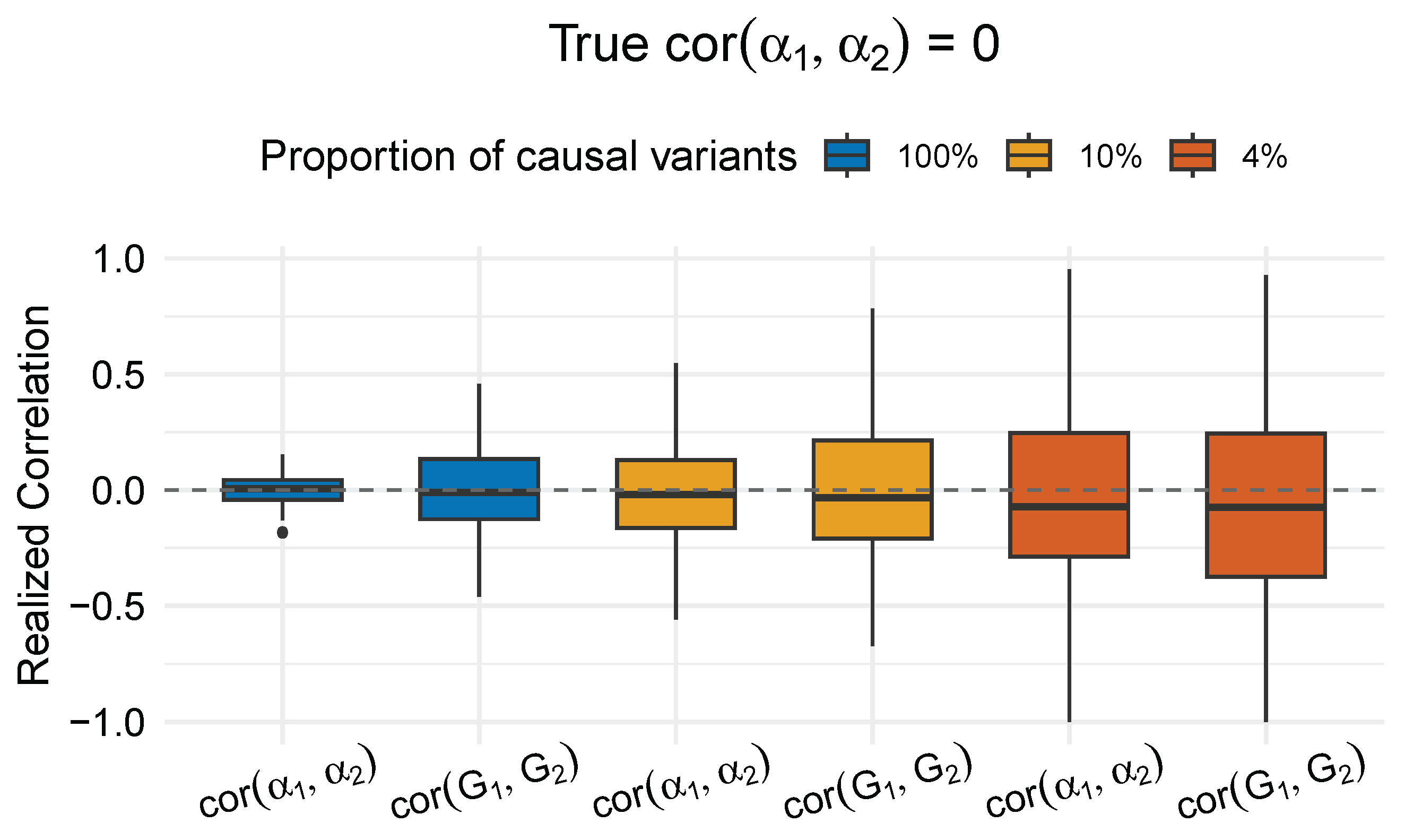
Figure 2R shows that smaller proportions of causal variants would generate wider distributions of the realized correlations cor(

α_{1}, α_{2}

) and cor(

G_{1}, G_{2}

). Moreover, to maintain the specified heritability, the smaller proportion of causal variants must have larger genetic effects. Altogether, they lead to higher detection rates by LAVA, but this result is clearly a statistical artifact generated by a mixture of zero and larger nonzero effects, not by any genuine correlation between the genetic effects. Therefore, LAVA detects certain patterns of regional genetic effects, not genetic correlations.

(As seen in de Leeuw et al.’s Figure 1, under the null, HDL-L is not affected by such a mixture. Moreover, the appearance of higher “power” of LAVA vs HDL-L under non-null settings in the random-effects model is an invalid comparison, because LAVA is based on higher type-I error rates.)

Discussion

For the random effects model in de Leeuw et al.’s Figure 1, LAVA produces inflated type-I error under the null hypothesis

r_{g} = 0

, while HDL-L remains well-calibrated. They considered this inflation not as a flaw, but rather as a result of LAVA’s “power” to detect non-zero realized correlations. This interpretation is incorrect for the following reasons:

Valid testing requires calibration under a data-generating process. When simulating from a model with true genetic correlation $r_{g} = 0$ , the realized genetic components $G_{1} = X α_{1}$ and $G_{2} = X α_{2}$ will exhibit non-zero correlation purely due to stochastic variation, especially in small regions or with limited number of causal variants. A valid testing procedure must control type-I error under this null model – that is, it must not declare significance at a rate higher than the nominal level, regardless of fluctuations in observed correlations.
Inflated type-I error rate is not power. The assertion that the observed inflation in LAVA is due to “power” is misleading. Power refers to the probability of detecting a true effect when it exists. Under the null hypothesis $r_{g} = 0$ , there is no true effect to detect. Thus, any rejection of the null in this setting is a false positive. Mistaking sensitivity to random noise as “power” indicates a failure to properly model uncertainty in the null distribution.
Artificial orthogonality does not address the problem. de Leeuw et al. suggest that when subject-level orthogonality is enforced – that is, when $cor (G_{1}, G_{2}) = 0$ is forced in simulations, LAVA’s calibration improves. While true, this is not a valid argument. In real data, the subject-level correlation under the null of no genetic effects will never be zero. A robust method must accommodate such fluctuations and remain conservative. HDL-L achieves this by modeling the variance of the local covariance estimator, thereby avoiding inflation under the null.
Counterintuitive type-I error inflation for a small proportion of causal variants. We observed that type-I error inflation in LAVA worsens for a smaller proportion of causal variants, even when the true genetic correlation remains zero. Two factors are involved: (i) the mixture of zero and sparse nonzero effects tends to produce higher realized correlations, and, (ii) to maintain a specified heritability, the smaller proportion of causal variants are assigned larger genetic effects. Overall, the fact that LAVA becomes more inflated in these settings suggests that its test statistic is overly sensitive to the presence of a genetic effect, regardless of whether the signal is shared across traits.

Author Contributions

X.S. and Y.P. initiated and supervised the study. Y.L., Y.P., and X.S. performed the analysis. All the authors contributed to the manuscript writing.

Data Availability Statement

The individual-level genotype data are available by application via the UK Biobank at https://www.ukbiobank.ac.uk.

Code Availability

The source code for reproducing the simulations and figures in this manuscript is available at https://github.com/YuyingLi-X/HDL-L/tree/main/Response.

Acknowledgments

X.S. was supported by a National Natural Science Foundation of China (NSFC) grant (No. 12171495), a National Key Research and Development Program grant (No. 2022YFF1202105), and a Swedish Research Council (Vetenskapsrådet) grant (No. 2022-01309).

Conflicts of Interest

The authors declare no competing interests.

References

de Leeuw, C., Werme, J. & Posthuma, D. Re-evaluating local genetic correlation analysis in the hdl framework. Preprints (2025). [CrossRef]
Werme, J., van der Sluis, S., Posthuma, D. & de Leeuw, C. A. An integrated framework for local genetic correlation analysis. Nature Genetics 54, 274–282 (2022). [CrossRef]
Li, Y., Pawitan, Y. & Shen, X. An enhanced framework for local genetic correlation analysis. Nature Genetics 57, 1053–1058 (2025). [CrossRef]
Lynch, M., Walsh, B. et al. Genetics and Analysis of Quantitative Traits, vol. 1 (Sinauer Sunderland, MA, 1998). See Chapters 26 and 27 for a detailed description of general mixed models.
Bulik-Sullivan, B. K. et al. LD Score regression distinguishes confounding from polygenicity in genome-wide association studies. Nature Genetics 2015, 47, 291–295. [CrossRef] [PubMed]
Bulik-Sullivan, B. et al. An atlas of genetic correlations across human diseases and traits. Nature Genetics 2015, 47, 1236–1241. [CrossRef] [PubMed]

Disclaimer/Publisher’s Note: The statements, opinions and data contained in all publications are solely those of the individual author(s) and contributor(s) and not of MDPI and/or the editor(s). MDPI and/or the editor(s) disclaim responsibility for any injury to people or property resulting from any ideas, methods, instructions or products referred to in the content.

© 2025 by the authors. Licensee MDPI, Basel, Switzerland. This article is an open access article distributed under the terms and conditions of the Creative Commons Attribution (CC BY) license (http://creativecommons.org/licenses/by/4.0/).

Copyright: This open access article is published under a Creative Commons CC BY 4.0 license, which permit the free download, distribution, and reuse, provided that the author and preprint are cited in any reuse.