
Submitted:
11 August 2025
Posted:
13 August 2025
You are already at the latest version
Abstract
This paper investigates the extension of the block-scaling approach—originally developed for estimating classifier accuracy—to uncertainty quantification in image classification tasks, where predictions accompanied by high confidence scores are generally more reliable. The proposed method involves applying a sliding mask filled with noise pixels to occlude portions of the input image and repeatedly classifying the masked images. By aggregating predictions across input variants and selecting the class with the highest vote count, a confidence score is derived for each image. To evaluate its effectiveness, we conducted experiments comparing the proposed method to MC dropout and a vanilla baseline using image datasets of varying sizes and levels of distortion. The results indicate that while the proposed approach does not consistently outperform alternatives under standard (in-distribution) conditions, it demonstrates clear advantages when applied to distorted and out-of-distribution samples. Moreover, combining the proposed method with MC dropout yields further improvements in both predictive performance and calibration quality in these more challenging scenarios.
Keywords:
deep learning
; block scaling quality
; uncertainty quantification
; confidence score
1. Introduction
Supervised learning is a core area of machine learning, primarily used to predict labels (or classes) for previously unseen data samples [1]. Before a model can be deployed, it must be trained. In a typical setup, a portion of the labeled dataset is allocated for training, while the remaining samples are reserved for testing and evaluating the model’s performance. This approach commonly assumes that real-world, unlabeled data shares a similar distribution with the training data. Under this assumption, strong test accuracy provides confidence that the model will generalize well and remain effective in practical applications.
In many practical applications—particularly in image recognition—the assumption that test samples follow the same (or similar) distribution as training samples often breaks down due to the dynamic and diverse nature of real-world environments. For instance, if a model is trained solely on images of white cats and gray dogs, as illustrated in Figure 1(a), it may incorrectly classify a gray cat (Figure 1(b)) as a dog. From the model’s perspective, white and gray cats exhibit different distributions, despite belonging to the same class.
In many scenarios, users cannot control the diversity of input data or restrict the training set to specific types of images such as white cats and gray dogs. This leads to a challenge known as the open set recognition (OSR) problem [2]. A conventional trained classifier assigns a label to every input sample, even if it does not belong to any of the known categories. As a result, the model tends to select the closest matching class instead of expressing uncertainty, which can undermine precision and degrade performance. For example, a white bear might be misclassified as a cat simply because both are white.
To address this issue, it becomes essential for models to provide confidence scores alongside classification results. A high confidence score suggests the prediction is reliable and can be accepted. Conversely, a low confidence score may signal the need for post-processing strategies—such as reclassification using alternative models or rejecting the sample outright as an outlier to known classes. The science of characterizing and quantifying uncertainties in computational models and predictions is known as uncertainty quantification (UQ).
Confidence estimation for input samples is an essential component of modern machine learning. Several approaches have been proposed to compute confidence scores, including the maximum softmax value (referred to as the vanilla method) [3], temperature scaling [4], deep ensemble [5], stochastic variational inference (SVI) [6], and Monte Carlo (MC) dropout [7]. Each method presents its own trade-offs. For example, SVI requires specialized network architectures that are not widely adopted, making implementation more complex—even when source code is available. Temperature scaling relies on training a separate parameter and has shown limited performance in comparative studies [8], including on standard datasets like MNIST [9].
Although deep ensemble methods can leverage conventional architectures, they require multiple models to average predictions, making confidence estimation computationally expensive and resource-intensive. This is problematic for users who rely on readily available pretrained models, as training multiple instances of the same architecture solely for confidence scoring may be impractical, especially in resource-constrained settings.
This study addresses the challenge of computing confidence scores using a single, possibly pretrained model. Our focus is on image recognition, a domain with wide-ranging applications—from traffic sign and road condition analysis in autonomous driving, to facial recognition in security systems, and even medical diagnosis via imaging.
In image recognition, test datasets may be categorized as:
- In-distribution: Samples closely resemble the training data (e.g., images of white cats or gray dogs in the previous example).
- Distorted in-distribution (distribution shift): Samples exhibit visual perturbations such as blur or color shift (e.g., gray cats viewed as distorted variants).
- Out-of-distribution (OOD): Samples differ entirely from training data, including unseen categories (e.g., white bears) or synthetic noise.
Building upon the Block Scaling Quality (BSQ) framework introduced by You, et al. [10]—which estimates model accuracy over test sets—this study extends BSQ to evaluate confidence scores for image classification. Both approaches operate under a shared conceptual foundation.
The main contributions of this paper are:
- Proposal of a confidence score based on block-scaling: A novel method for quantifying sample uncertainty using BSQ. This approach requires only one model and supports the use of pretrained networks.
- Experimental comparison: Evaluation of the proposed approach against MC dropout and vanilla approaches under in-distribution, distorted, and OOD datasets. Empirical results show that our method offers superior performance under distortion and OOD conditions.
2. Related Work
Hendrycks and Gimpel [3] investigated the use of the maximum softmax value (vanilla) as a baseline for detecting misclassified and OOD samples. Their study employed two widely used evaluation metrics: the Area Under the Receiver Operating Characteristic Curve (AUROC) and the Area Under the Precision-Recall Curve (AUPR). Results showed that the vanilla baseline performed effectively across a variety of test datasets. Accordingly, this method is included as a comparison target in our subsequent experimental analysis.
Guo et al. [4] found that neural networks often exhibit poor calibration, with predictive confidence misaligned from true accuracy. Their analysis revealed that factors such as network depth, the number of hidden units, and the use of batch normalization contribute to this miscalibration. To address this issue, they proposed a simple yet effective post-processing technique known as temperature scaling, which applies a single-parameter adjustment to the logits to calibrate the predicted probabilities.
Lakshminarayanan et al. [5] introduced the deep ensemble approach, which employs multiple identical neural networks to generate independent predictions. The confidence score for a given input is obtained by averaging the softmax outputs across the ensemble. According to comparative analyses [8], this method demonstrates relatively stronger performance in both classification accuracy and uncertainty quantification. A conceptually related approach was proposed by You et al. [11], whose primary objective was to estimate model prediction accuracy over a test set without access to ground-truth labels.
The Bayesian neural network (BNN) [6] differs fundamentally from conventional neural networks in how it models uncertainty. While traditional neural networks learn deterministic weight parameters through optimization, BNNs treat each connection weight as a probability distribution, typically over plausible values conditioned on the training data. As a result, repeated predictions on the same input yield varying outputs, reflecting epistemic uncertainty. This stochasticity is analogous to ensembling multiple models, and it allows for the computation of confidence scores by aggregating outputs from multiple forward passes.
To estimate the confidence level of an unlabeled sample, Gal and Ghahramani [7] employed MC dropout with rate p on a trained neural network. This technique introduces stochasticity by randomly deactivating units and their corresponding weights during inference, effectively sampling from an approximate posterior over the model parameters. By performing multiple stochastic forward passes, an ensemble of predictive distributions is generated. Similar to deep ensembles, the confidence score is computed by averaging the softmax outputs across these passes, thereby capturing predictive uncertainty in the absence of ground-truth labels.
Ovadia et al. [8] conducted an extensive comparative study on the robustness of various uncertainty estimation techniques—including deep ensembles, Bayesian neural networks, and standard (vanilla) models—under dataset shift scenarios. Their findings indicate that deep ensembles, as previously described, outperform other methods across several performance and calibration metrics when confronted with distributional changes. Among the studied techniques, temperature scaling has shown limited performance in comparative studies. Some approaches necessitate model re-training or architectural modifications, rendering them unsuitable for pre-trained networks. Therefore, vanilla and MC dropout remain the only methods among those evaluated that can be directly applied to a pre-trained model. They are used in the comparison.
Abdar et al. [12] provided a comprehensive survey of recent advancements in UQ techniques, with particular emphasis on Bayesian-based and deep ensemble-based methods. Their work also reviewed the application of these approaches in reinforcement learning settings and identified key research challenges and future directions for the development of UQ frameworks.
Kristoffersson Lind et al. [13] examined various metrics for uncertainty quantification (UQ) in regression tasks, including area under the sparsification error curve, calibration error, Spearman’s rank correlation, and negative log-likelihood. Using multiple datasets, they found calibration error to be the most effective overall, while noting that other metrics remain valuable depending on the specific context.
3. Proposed Approach
Existing approaches to confidence estimation, such as deep ensemble and MC dropout, derive confidence scores by averaging multiple classification outputs for a given input sample. In deep ensemble methods, multiple models are individually trained; in MC dropout, stochastic predictions are produced by randomly deactivating internal neurons during inference. In contrast, this paper proposes a novel method that generates multiple classification outcomes by applying localized perturbations directly to the input image—an approach conceptually similar to dropout, but at the input level.
In the following, lowercase variables denote scalars, while uppercase variables represent matrices. Lowercase subscripts indicate indices, whereas uppercase subscripts correspond to constants. For notational shorthand, abbreviations using two or more capital letters—such as CS for confidence score—are adopted in equations.
As shown in Figure 2, the proposed approach consists of the following steps:
- Generation of image masks. We define a mask , where and denote mask dimensions. Each pixel in the mask receives independently sampled uniform values across the red, green, and blue channels, allowing diverse contextual substitution when overlayed onto the original image. Typically, the mask size is approximately the size of the input image. Empirical observations suggest that mask size has limited impact on final performance.
- Construction of masked images. For a single test image , we generate variants by sliding the mask from bottom-left to top-right. Specifically, let the bottom-left corner of the mask be initialized at location at ( for the s-th test image. Then, the pixel values of are computed as:
- Classifications of generated images. Each masked image is passed through the classification model to obtain a softmax output , where is the total number of classes. Overall, there are sets of .
- Majority voting for class prediction. Initially, let for . For each prediction, let the predicted class be . we then update the vote count such that . The final class label for the original image I is determined by majority vote as .
- Confidence score computation. We then compute the mean and standard deviation across the softmax scores for class from the masked images, where and . Here, reflects the model’s average confidence, while captures its sensitivity to localized perturbations. A low implies stable predictions; a high suggests the model relies on spatially localized features. To map these values to a normalized confidence score in [0, 1], we apply a scaling function based on the arctangent of the inverse variance. The final confidence score is calculated as:where [0,1] is a weighting factor balancing average confidence and sensitivity-based adjustment.
4. Experiments and Results
This section presents the experimental setup and corresponding results. It begins with a description of the evaluation metrics used in the analysis, followed by brief overviews of the datasets and baseline comparison targets. Subsequently, the models employed in the experiments are introduced. Five experiments are conducted: four on individual datasets and one additional experiment demonstrating the feasibility of an ensemble strategy. The section concludes with a summary of key findings.
4.1. Evaluation Metrics
Evaluation metrics are used to assess whether uncertainty quantification accurately reflects the relationship between a model’s confidence scores and actual outcomes. Below we discuss the metrics used in this paper.
4.1.1. Accuracy vs. Confidence Curve
The accuracy vs. confidence curve is a commonly used tool in machine learning and statistical analysis for evaluating how well a model’s prediction confidence aligns with its empirical accuracy. In this curve, the confidence denotes the probability score a model assigns to its prediction (e.g., a score of 0.6 reflects a 60% belief that the prediction is correct). The accuracy represents the proportion of correct predictions within a given confidence threshold. The curve plots cumulative accuracy across various confidence levels to reveal calibration behavior.
For binary classification, the x-axis corresponds to the confidence threshold , while the y-axis denotes the cumulative accuracy (CA), computed as:
where is the total number of test samples, is an indicator function returning 1 if the condition holds and 0 otherwise, is the model’s predicted probability for the true class given input , and is the predicted class label for sample . In the actual implementation of multi-class classification scenarios, is the softmax value of the true class , i.e., . In our experimental analysis, we focus on the high-confidence region of the accuracy-confidence curve to assess model reliability. For a given confidence score, a higher corresponding accuracy indicates stronger predictive calibration and is therefore preferable.
4.1.2. Expected Calibration Error (ECE)
Expected calibration error (ECE) quantifies how well a model’s predicted confidence scores align with true outcomes [14]. Ideally, a confidence score of 60% should correspond to a 60% chance that the associated prediction is correct. To compute ECE, model predictions are partitioned into bins based on confidence scores. Each bin , where , contains samples with confidence values falling within the interval . For each bin, let denote the average confidence and the empirical accuracy. Then, ECE is defined as:
where is the number of samples in bin , and is the total number of test samples.
A lower ECE value indicates better calibration—i.e., the model’s confidence scores more accurately reflect the likelihood of correctness. However, it is important to note that a lower ECE does not necessarily imply higher classification accuracy; calibration and accuracy are related but distinct properties [15].
4.1.3. Brier Score
The Brier score (BS) [16] is a metric for evaluating the accuracy of probabilistic predictions in both binary and multi-class classification settings. It computes the mean squared error between the predicted probability distributions and the true class labels.
Let denote the predicted probability that sample belongs to class , and let indicate whether truly belongs to class (i.e., for the correct class, and 0 otherwise). The Brier score is defined as:
In practice, the model output is used in place of , representing the softmax probability for classon sample . Similar to ECE, lower Brier scores indicate better calibrated and more accurate probabilistic predictions. However, BS simultaneously reflects both calibration and sharpness, making it a more holistic measure in some evaluation contexts.
4.1.4. Negative Log-Likelihood
Negative log-likelihood (NLL) [17] is a widely-used loss function in classification tasks and probabilistic modeling. It quantifies how well the predicted probability distribution aligns with the true class labels, with the objective of maximizing the likelihood of the observed data under the model’s distribution.
In the multi-class setting, the NLL is calculated based on the predicted probability assigned to the correct class label for each sample. Let be the predicted probability that sample belongs to the true class . Then, the NLL is defined as:
In practice, the model typically uses the softmax activation function for outputs . Therefore, for each sample , the term is taken as , where corresponds to the true label.
Similar to metrics like ECE and the BS, a lower NLL indicates better predictive performance. However, unlike BS which reflects both calibration and sharpness, NLL is directly tied to likelihood optimization and penalizes overconfident incorrect predictions more severely.
4.1.5. Entropy
Entropy (EN), rooted in information theory [18], quantifies the uncertainty inherent in a probability distribution. Higher entropy values indicate greater unpredictability or “disorder” in model predictions. In the context of OOD detection, it is desirable for the confidence scores assigned to all classes to be nearly uniform—signifying that the model cannot make a definitive prediction and is appropriately expressing uncertainty.
For each test sample , entropy is computed as:
where is the number of classes and denotes the predicted softmax probability for class on sample .
A higher entropy value implies that the prediction distribution is flatter and less confident—an outcome that is preferable for identifying OOD samples. This metric serves as an effective proxy for gauging model uncertainty in scenarios where the input may not belong to any of the known classes.
4.1.6. Using the Metrics in Experiments
Table 1 provides an overview of all evaluation metrics used in this study. A notable limitation emerges for metrics that inherently rely on probabilistic distributions—specifically, BS, NLL, and entropy. These metrics are not applicable to the proposed confidence score, which is constructed from the mean and standard deviation of softmax outputs. Because this representation deviates from a probability distribution, it breaks the probabilistic assumptions underlying those metrics.
This limitation affects the final two steps of the proposed method, where the derived confidence scores no longer retain a direct probabilistic interpretation. Unlike raw softmax probabilities, which sum to one and represent a categorical distribution, the mean–standard deviation formulation represents a statistical summary that cannot be meaningfully evaluated using metrics designed for full distributions.
In this study, Accuracy vs. Confidence Curve and ECE are employed as the primary evaluation metrics. These metrics do not assume probabilistic normalization—such as softmax—of model outputs, making them well-suited for assessing the reliability of the proposed confidence scores. Importantly, both metrics evaluate whether high-confidence predictions correspond to high empirical accuracy, providing meaningful insight into the effectiveness of the uncertainty quantification.
Although Brier Score and NLL are not directly applicable to the proposed confidence scores—given that they require probabilistic distributions—they offer valuable complementary perspectives. To facilitate comparison using these metrics, only the first three steps of the proposed method are carried out, and the average softmax output across masked images is used in the computation. These metrics are thus categorized as secondary and used to provide a broader analysis of model behavior.
For OOD samples, where ground-truth labels are unavailable, entropy is adopted as the evaluation criterion. For the same reason as in Brier score and NLL, we choose to apply it to softmax outputs derived from steps 1–3 of our approach to maintain a fair basis for comparison with other methods.
4.2. Experimental Datasets
This subsection introduces the datasets used in the experiments. From the selected datasets, distorted in-distribution variants are generated to simulate distribution shift. Additionally, OOD datasets are incorporated to evaluate model behavior under unfamiliar conditions.
Among the datasets, CIFAR-10 [19,20] and ImageNet 2012 [21,22] were previously employed in Ovadia et al. [8], and are thus included for consistency and comparative evaluation. Since the final step of our proposed method—confidence score calibration—was partially guided by performance insights derived from these two datasets, we additionally introduce two benchmark datasets that were not used in developing the confidence score methodology. This ensures an impartial comparison and robust evaluation of the proposed approach across both familiar and unseen data distributions.
4.2.1. CIFAR-10
CIFAR-10 [19,20] is a widely used benchmark in image classification research. It comprises labeled images spanning ten categories, including common animals and vehicles, and serves as a standard testbed for evaluating the performance of machine learning and deep learning models. Developed by Alex Krizhevsky, Vinod Nair, and Geoffrey Hinton, the dataset was released through the Canadian Institute for Advanced Research (CIFAR). Detailed specifications are provided in Table 2.
4.2.2. ImageNet 2012
ImageNet 2012 [21,22] is a large-scale image classification dataset, best known as the foundation for the ImageNet Large Scale Visual Recognition Challenge (ILSVRC). It plays a pivotal role in advancing machine learning and deep learning research, particularly in high-performance image classification.
Developed jointly by Stanford University and Princeton University as part of the broader ImageNet project, the dataset leverages the hierarchical structure of WordNet, wherein each category corresponds to a set of synonyms (Synsets). The dataset includes a wide spectrum of image categories encompassing animals, vehicles, everyday objects, and natural landscapes. These specifications—outlined in Table 3—make ImageNet 2012 a cornerstone benchmark for evaluating the scalability and generalizability of image recognition models.
4.2.3. iNaturalist 2018
iNaturalist 2018 [23,24] is a large-scale image classification dataset curated for biodiversity-focused machine learning research. Originating from the iNaturalist platform and organized by the Visipedia team, the dataset was featured in the CVPR FGVC5 competition.
It contains images categorized by biological species and further grouped into super-categories to facilitate hierarchical classification. Detailed specifications are listed in Table 4. Given its structure and taxonomic diversity, iNaturalist 2018 is well-suited for tasks such as species identification, biological classification, and deep learning model evaluation. In our experiments, we utilize only the superclass labels to simulate a reduced-class scenario. Notably, this setup introduces a pronounced class imbalance, which adds further complexity to model calibration and evaluation.
4.2.4. Places365 Dataset
Places365 [25,26] is a large-scale scene recognition dataset curated by the MIT Computer Science and Artificial Intelligence Laboratory (CSAIL). It is primarily used in image classification and scene understanding tasks and serves as a standard benchmark in machine learning and deep learning research.The dataset is a subset of the broader Places2 Database and is available in two variants: Places365-Standard and Places365-Challenge. Detailed specifications are provided in Table 5.
A distinctive characteristic of Places365 is its inclusion of images with rich co-occurring object structures. For example, a kitchen scene might feature a stove, refrigerator, sink, and tableware, while other categories—such as classrooms or libraries—are defined not only by the presence of objects but also by their spatial and functional arrangement. These structured patterns offer valuable semantic cues, making Places365 particularly effective for evaluating models that incorporate contextual and spatial reasoning.
4.2.5. Distorted in-Distribution Datasets
In addition to the primary datasets—CIFAR-10, ImageNet 2012, iNaturalist 2018, and Places365—this study incorporates distorted variants to evaluate model performance under various degradation scenarios. For CIFAR-10 and ImageNet 2012, the existing corrupted versions (CIFAR-10-C and ImageNet-C) are directly adopted.
However, as no predefined distortion sets are available for iNaturalist 2018 and Places365, this study extends the ImageNet-C distortion transformation framework to generate analogous corrupted samples for these two datasets. The implemented distortion functions are summarized in Table 6, with visual illustrations of the corresponding image alterations provided in Figure 3. Notably, the Frost transformation could not be replicated for iNaturalist 2018 and Places365 due to the absence of the original reference images necessary for applying this specific effect.
4.2.6. Out-of-Distribution Datasets
For CIFAR-10, the SVHN dataset is selected as its OOD counterpart. In contrast, ImageNet 2012, iNaturalist 2018, and Places365 are paired with synthetically generated random RGB images of resolution 224 × 224 pixels to serve as OOD samples.
Given the wide range of semantic categories covered by the experimental datasets, random noise images provide an effective proxy for extreme OOD cases—where the test inputs are entirely dissimilar to any of the known classes. Furthermore, the proposed method operates on masked patches, which also involve random noise. As such, distinguishing between unaltered and corrupted regions becomes particularly challenging when the OOD inputs themselves are purely noise-based, thus presenting a stringent evaluation scenario.
4.3. Comparison Targets
The baseline models used for comparison include: (1) a vanilla approach that relies directly on softmax outputs as confidence scores, and (2) the MC dropout method. In the experimental setup, following the protocol in [8], the dropout probability is fixed at 0.05 without modification. This enables direct reuse of the results reported in [8], thereby alleviating the need for retraining and reducing computational overhead.
4.4. Model Architectures and Configuration
To ensure a fair comparison with the results reported in [8], the deep learning models for CIFAR-10 and ImageNet 2012 follow the same architectural designs outlined in that reference. However, a notable distinction lies in the training strategy for ImageNet 2012: instead of training from scratch, models in this study leverage the official pretrained weights provided by PyTorch [27], consistent with widely adopted best practices.
For the iNaturalist 2018 and Places365 datasets, this study introduces additional configuration details. The iNaturalist 2018 models are trained using the hyperparameter settings specified in Table 7, while the Places365 models employ pretrained weights released by the MIT CSAIL team [28], also documented in Table 7.
To support the implementation of the proposed method, additional configuration parameters are specified in Table 8. Due to the large scale of several experimental datasets—particularly ImageNet 2012, iNaturalist 2018, and Places365—subsampling is applied to reduce training time and computational overhead. The numbers of sampling images are also documented in Table 8.
4.5. Experiment I: CIFAR-10
The objective of this experiment is to assess the effectiveness of the proposed uncertainty quantification method on a small-scale image classification task, using CIFAR-10 as the in-distribution benchmark. The evaluation focuses on both predictive accuracy and calibration quality, and compares the proposed approach with existing techniques.
Table 9 presents the comparative results using various uncertainty quantification metrics. For baseline methods—including MC dropout and vanilla softmax confidence—the reported values are extracted directly from figures in [8], without retraining, to ensure alignment and fair comparison. Therefore, NLL is not available to report here.
The results indicate that the proposed method does not yield a performance advantage over MC dropout on CIFAR-10. A possible explanation lies in the data augmentation strategy adopted during training: the base model already utilizes techniques such as random cropping, which introduces spatial variability by exposing the network to different subregions of each image. This enhances the model’s spatial robustness and reduces its sensitivity to perturbations introduced through random masking—the core mechanism of the proposed confidence score estimation. Consequently, the masking operation may not sufficiently disrupt the model’s inference behavior, leading to less informative uncertainty measurements.
While the proposed method does not outperform MC dropout under standard conditions (e.g., the CIFAR-10 test set), its advantages become more evident in the presence of input degradation. For example, under moderate distortion—specifically Gaussian blur level 3 in CIFAR-10-C—the cumulative accuracy within high-confidence prediction regions surpasses that of MC dropout, as shown in Figure 4, indicating stronger uncertainty quantification.
Furthermore, as distortion severity increases, the proposed method consistently exhibits lower ECE, emphasizing its enhanced calibration capability under degraded conditions. This pattern, visualized in Figure 5, suggests that the method is more effective in predictive uncertainty when faced with challenging inputs.
In summary, although performance on clean data remains comparable or slightly below baseline, the proposed approach demonstrates superior robustness and uncertainty sensitivity in adverse scenarios, making it a promising candidate for calibration-aware modeling in real-world settings where input quality may vary.
In scenarios involving out-of-distribution inputs, the proposed method yields more pronounced uncertainty responses than MC Dropout, as depicted in Figure 6. Specifically, the mode of the predictive entropy under the proposed approach reaches 1.066, compared to approximately 0.976 for MC Dropout. This higher entropy concentration indicates a more cautious predictive behavior, suggesting that the proposed method is less likely to assign overconfident predictions to samples outside the CIFAR-10 training distribution.
By generating sharper entropy distributions for OOD inputs, the method demonstrates improved awareness of epistemic uncertainty and a reduced tendency to overfit unfamiliar data. This characteristic is essential for safe model deployment in open-world settings, where unseen or corrupted inputs may arise unexpectedly.
4.6. Experiment II: ImageNet 2012
To assess the scalability and robustness of the proposed uncertainty quantification method, we extend our evaluation to large-scale image classification datasets, including ImageNet 2012, ImageNet-C, and a custom-designed set of OOD samples.
Evaluation metrics on in-distribution datasets, presented in Table 10, reveal comparable performance between the proposed method and MC Dropout. For distorted samples—particularly under Gaussian blur level 3 in ImageNet-C—both approaches exhibit similar cumulative accuracy-confidence characteristics in the high confidence region, as depicted in Figure 7.
Notably, as distortion severity increases, the ECE trend under the proposed method exhibits markedly greater consistency, as shown in Figure 8. This pattern highlights enhanced calibration stability in scenarios with degraded input quality. Such resilience suggests that the method more effectively quantifies predictive uncertainty when confronted with heavily corrupted data, thereby mitigating the risk of erroneous high-confidence predictions in ambiguous or noisy conditions.
Regarding OOD inputs, the proposed method displays quantitative advantages over MC dropout, as shown in Figure 9; however, its entropy distribution notably overlaps with that of the Vanilla baseline. This phenomenon can be attributed to the behavior of vanilla softmax when confronted with highly unfamiliar inputs—such as randomly generated three-channel RGB images—across a large number of output classes. In such cases, vanilla tends to produce nearly uniform softmax scores, resulting in elevated predictive entropy despite lacking true uncertainty awareness.
Conversely, while the proposed method integrates a masking mechanism designed to induce uncertainty, its behavior on highly abnormal samples can lead to concentrated activations in specific output branches. This effect suppresses the tails of the entropy distribution, reducing sensitivity at its extremes. As a result, although the method retains uncertainty quantification capabilities, its response to severe OOD samples may exhibit limitations in entropy expressiveness.
4.7. Experiment III: iNaturalist 2018
The iNaturalist 2018 dataset presents a long-tailed image classification challenge due to its highly imbalanced class distribution. Under standard (in-ddistribution) evaluation protocols, the proposed method outperforms MC dropout, as illustrated in Figure 10. This improvement is chiefly attributed to the fundamental differences in uncertainty modeling: while MC dropout relies on repeated stochastic neuron masking, leading to prediction variance and diminished stability, the proposed technique mitigates these disruptions. As a result, it achieves superior robustness and interpretability in uncertainty quantification.
However, in terms of ECE and other metrics, our method slightly underperforms compared to the vanilla approach, as shown in Table 11. This suggests that although the vanilla method lacks explicit uncertainty quantification mechanisms, its calibration accuracy remains competitive in scenarios with significant class imbalance.
Under distortion conditions in the iNaturalist 2018 dataset, the proposed method demonstrates significant advantages over both MC dropout and vanilla approaches, especially for high confidence levels, as shown in Figure 11. Furthermore, regarding the distribution of ECE values for all level-3 distortions, the proposed method yields the lowest median, as shown in Figure 12, indicating stable calibration performance. To save simulation time, only datasets with level-3 distortion are used in the calculation. These results validate the method’s effectiveness in uncertainty quantification under conditions of severe class imbalance and substantial input distortion.
Under OOD conditions, the proposed method demonstrates more discerning uncertainty characteristics on the iNaturalist 2018 dataset. Despite the pronounced class imbalance—which induces a bias toward certain classes and results in an overall low-entropy distribution—both our method and vanilla achieve meaningful sample concentration within the higher-entropy region, as depicted in Figure 13. In contrast, MC dropout exhibits strong concentration in the low-entropy region, suggesting a tendency toward overconfident predictions and diminished reliability in uncertainty quantification.
4.8. Experiment IV: Places365
Compared to ImageNet, the Places365 dataset is distinguished by its high semantic density and visually complex backgrounds. As such, models trained on Places365 must capture holistic scene context rather than relying solely on localized object features. Under in-distribution evaluation, the proposed method does not demonstrate a marked advantage over either MC dropout or the baseline vanilla approach, as reflected in Figure 14 and Table 12.
Under Gaussian-3 distortion conditions, the proposed method exhibits only minor gains over MC dropout and the vanilla approach in terms of confidence–accuracy alignment (Figure 15). However, it demonstrates improved performance in ECE for all level-3 distortions, as shown in Figure 16, indicating enhanced calibration robustness in the presence of degraded visual quality and semantically complex imagery.
In the OOD scenario for the Places365 dataset, depicted in Figure 17, all methods yield predictions with moderate confidence levels, reflected in entropy values significantly below the theoretical upper bound of log (365) ≈ 5.9 nats. However, the proposed method exhibits a more distinct concentration of samples in the higher-entropy region compared to other approaches, suggesting enhanced capability in expressing elevated uncertainty for OOD inputs.
4.9. Experiment V: Ensemble Approaches
Given the distinct mechanisms employed by our proposed method and the MC dropout technique for computing confidence scores, it is feasible to combine their outputs in an ensemble-like fashion. To explore this possibility, we use the Places365 dataset as a case study.
The integration procedure involves two steps: first, the input image is processed using the proposed method to determine the predicted class (via majority voting) and its associated confidence score. Then, the same input is evaluated using MC dropout to compute a confidence score for the same predicted class. These two scores are averaged to obtain a final ensemble-based confidence value.
The results for this hybrid approach—evaluated on the original Places365 dataset—are presented in Figure 18. However, as shown, the combined method does not yield performance improvements over either standalone technique. Since this ensemble strategy targets score fusion rather than predictive refinement, only ECE is reported in Table 13. The ensemble approach does not have a clear advantage, suggesting limited synergy between the two underlying confidence estimation mechanisms for in-distribution samples.
In scenarios involving distorted inputs, the ensemble approach exhibits improved calibration performance—underscoring one of the key strengths of the proposed method. As illustrated in Figure 19, the ensemble technique achieves higher accuracy within the high-confidence prediction region, making it a preferable strategy under such conditions.
Further evidence is provided in Figure 20, which presents the ECE results for level-3 distortion. The ensemble method yields a lower median error and narrower distribution intervals, highlighting its ability to maintain robust uncertainty quantification even under significant image degradation. These findings affirm the practical value of integrating the proposed method with MC dropout to enhance reliability and performance in challenging visual environments.
In OOD scenarios, the ensemble approach demonstrates a clear advantage over other methods, as illustrated in Figure 21. This underscores the combined method’s superior capability to quantify uncertainty in OOD samples enriched with contextual information.
4.10. Summary of Experimental Results
- We conducted four experiments (Subsections 4.5–4.8) to evaluate the relative performance of the proposed approach, MC dropout, and vanilla baseline methods. One additional experiment (Subsection 4.9) explored the feasibility of fusing two confidence scores. The findings are summarized as follows:
- In-distribution datasets: The proposed method demonstrates consistently stable performance, remaining comparable to the other two approaches. While it does not consistently outperform them, its reliability underscores its effectiveness in standard settings.
- Distorted (distribution-shift) datasets: In high-confidence regions, the proposed method achieves higher cumulative accuracy and lower ECE, indicating stronger calibration performance and heightened sensitivity to data degradation.
- OOD datasets: The method exhibits a denser concentration of samples in high-entropy regions, effectively reducing overconfident predictions and enhancing the model’s awareness of unfamiliar inputs.
- Class-imbalanced datasets (e.g., iNaturalist 2018): Relative to the other two methods, the proposed approach better mitigates prediction bias arising from unstable dropout, demonstrating enhanced robustness and interpretability.
- Ensemble performance: When integrated with MC dropout, the proposed method performs notably well under distortion scenarios, achieving lower ECE and a higher entropy peak center value than either method in isolation—highlighting its potential for synergistic integration.
5. Conclusions
This paper investigates the performance of the proposed uncertainty quantification method again MC dropout and vanilla across diverse image datasets, including standard (in-distribution) datasets with varying numbers of classes, distorted datasets, and OOD datasets. The analysis further extends to datasets characterized by extreme class imbalance and semantic complexity, as well as to the heterogeneous integration of the proposed method with MC dropout. Experimental results demonstrate that the proposed method consistently outperforms MC dropout and the vanilla baseline in handling heavily distorted inputs and OOD samples. Moreover, its heterogeneous integration with MC dropout further elevates predictive performance and calibration quality in these challenging scenarios.
Future work will explore extending the proposed approach to input-level uncertainty quantification in large language models, with a focus on examining how semantic masking influences language comprehension and predictive confidence. By incrementally masking segments of the input text and tracking corresponding changes in confidence scores, a conceptually analogous framework to the current method can be applied to assess sensitivity and calibration at the input level.
Supplementary Materials
After paper accepted, the source code for the experiments can be downloaded at: https://github.com/NTUT-LabASPL2.
Author Contributions
Conceptualization, S.D.Y.; methodology, P.X.W., C.H.L. and S.D.Y.; software, P.X.W.; validation, P.X.W., C.H.L. and S.D.Y.; formal analysis, S.D.Y.; investigation, P.X.W., C.H.L. and S.D.Y.; resources, C.H.L. and S.D.Y.; data curation, P.X.W.; writing—original draft preparation, S.D.Y.; writing—review and editing, C.H.L.; visualization, P.X.W.; supervision, C.H.L. and S.D.Y.; project administration, C.H.L. and S.D.Y.; funding acquisition, C.H.L. All authors have read and agreed to the published version of the manuscript.
Funding
This research was funded by National Science and Technology Council, Taiwan, grant number NSTC 112-2221-E-027-049-MY2. The APC was waived by invitation. https://github.com/NTUT-LabASPL2/BrainMRI.
Institutional Review Board Statement
Not applicable.
Informed Consent Statement
Not applicable.
Data Availability Statement
Experimental datasets are from 3rd party and are publicly available. See text for details.
Acknowledgments
During the preparation of this manuscript, the authors used Copilot for the purposes of generating Figure 1 and polishing English writing. The authors have reviewed and edited the output and take full responsibility for the content of this publication.
Conflicts of Interest
The authors declare no conflicts of interest. The funders had no role in the design of the study; in the collection, analyses, or interpretation of data; in the writing of the manuscript; or in the decision to publish the results.
Abbreviations
The following abbreviations are used in this manuscript:
| BNN | Bayesian Neural Network |
| BSQ | Block Scaling Quality |
| ECE | Expected Calibration Error |
| MC | Monte Carlo |
| NLL | Negative Log-Likelihood |
| OOD | Out of distribution |
| UQ | Uncertainty Quantification |
References
- Mohri, M.; Rostamizadeh, A.; Talwalkar, A. Foundations of Machine Learning; The MIT Press: Cambridge MA, USA, 2012. [Google Scholar]
- Scheirer, W. J.; de Rezende Rocha, A.; Sapkota, A. and Boult, T. E. Toward open set recognition. IEEE Trans Pattern Anal Mach Intell. 2013, 35, 1757–1772. [Google Scholar] [CrossRef] [PubMed]
- Hendrycks, D.; Gimpel, K. A baseline for detecting misclassified and out-of-distribution examples in neural networks. In International Conference on Learning Representations, Toulon, France, 24 – 26 April 2017.
- Guo, C.; Pleiss, G.; Sun, Y.; Weinberger, K. Q. On calibration of modern neural networks. In International Conference on Machine Learning, Sydney, Australia, 6-11 August, 2017.
- Lakshminarayanan, B.; Pritzel, A.; Blundell, C. Simple and scalable predictive uncertainty estimation using deep ensembles. Adv. Neural Inf. Process. 2017, 30, 6405–6416. [Google Scholar]
- Blundell, C.; Cornebise, J.; Kavukcuoglu, K.; Wierstra, D. Weight uncertainty in neural networks. In International Conference on Machine Learning, Lille, France, 6-11 July 2015.
- Gal, Y.; Ghahramani, Z. Dropout as a Bayesian approximation: representing model uncertainty in deep learning. In International Conference on Machine Learning, New York City, NY, USA, 19-24 June 2016.
- Y. Ovadia et al. Can you trust your model’s uncertainty? Evaluating predictive uncertainty under dataset shift. Adv. Neural Inf. Process. 2019, 32, 13991–14002. [Google Scholar]
- MNIST Dataset. Available online: https://www.kaggle.com/datasets/hojjatk/mnist-dataset (accessed on 1 August 2025).
- You, S. D.; Lin, K-R; Liu, C-H. Estimating classification accuracy for unlabeled datasets based on block scaling. Int. j. eng. technol. innov. 2023, 13, 313–327. [Google Scholar]
- You, S. D.; Liu, H-C; Liu, C-H. Predicting classification accuracy of unlabeled datasets using multiple deep neural networks. IEEE Access, 2022, 10, 1–12. [Google Scholar] [CrossRef]
- M. Abdar, et al. A review of uncertainty quantification in deep learning: Techniques, applications and challenges. Information Fusion 2021, 76, 243–297. [Google Scholar] [CrossRef]
- Kristoffersson Lind, S.; Xiong, Z.; Forssén, P-E; Krüger, V. Uncertainty quantification metrics for deep regression. Pattern Recognit. Lett. 2024, 186, 91–97. [Google Scholar] [CrossRef]
- Pavlovic, M. Understanding model calibration - A gentle introduction and visual exploration of calibration and the expected calibration error (ECE). arXiv:2501.19047v2 2025, available at https://arxiv.org/html/2501.19047v2.
- Si, C.; Zhao C.; Min S.; Boyd-Graber, J. Re-examining calibration: The case of question answering. arXiv preprint arXiv:2205.12507, 2022, available at https://arxiv.org/pdf/2205.12507.
- Brier, G. W. Verification of forecasts expressed in terms of probability. Mon. Weather Rev. 1950, 78, 1–3. [Google Scholar] [CrossRef]
- Gneiting, T.; Raftery, A. E. Strictly proper scoring rules, prediction, and estimation. J. Am. Stat. Assoc. 2007, 102, 359–378. [Google Scholar] [CrossRef]
- Shannon, C. E. A mathematical theory of communication. Bell Syst. Tech. J. 1948, 27, 379–423. [Google Scholar] [CrossRef]
- Krizhevsky, A. Learning multiple layers of features from tiny images. University of Toronto, 2009.
- The CIFAR-10 Dataset. Available online: https://www.cs.toronto.edu/~kriz/cifar.html (accessed on 1 August 2025).
- Deng, J.; Dong, W.; Socher, R.; Li, L.-J.; Li, K.; Li, F-F. ImageNet: A large-scale hierarchical image database. In Proceedings of the 2009 IEEE Conference on Computer Vision and Pattern Recognition, Miami, FL, USA, 20-25 June 2009. [Google Scholar]
- Russakovsky, O.; et al. ImageNet large scale visual recognition challenge. Int. J. Comput. Vis. 2015, 115, 211–252. [Google Scholar] [CrossRef]
- Van Horn, G.; et al. The iNaturalist Species Classification and Detection Dataset. In Proceedings of the IEEE Conference on Computer Vision and Pattern Recognition (CVPR), Salt Lake City, Utah, USA, 18-22 June 2018. [Google Scholar]
- Visipedia/Inat_comp. Available online: https://github.com/visipedia/inat_comp (accessed on 1 August 2025).
- Zhou, B.; Lapedriza, A.; Khosla, A.; Oliva, A.; and Torralba, A. Places: A 10 million Image Database for Scene Recognition," IEEE Trans Pattern Anal Mach Intell. 2017, 40, 1452–1464.
- Places Download. Available online: http://places2.csail.mit.edu/download.html (accessed on 1 August 2025).
- Models and pre-trained weights. Available online: https://docs.pytorch.org/vision/main/models.html (accessed on 1 August 2025).
- CSAILVision/Places365. Available online: https://github.com/CSAILVision/places365 (accessed on 1 August 2025).
Figure 1.
Illustration of training (a) and test (b) samples.

Figure 2.
Illustration of the proposed approach. Step 1 (image mask generation) is omitted from the figure. In Step 2, the noise mask is depicted as a blue block. Steps 3 and 4 are merged, producing only two class outputs. The final step involves computing the confidence score using Equation 2.
Figure 2.
Illustration of the proposed approach. Step 1 (image mask generation) is omitted from the figure. In Step 2, the noise mask is depicted as a blue block. Steps 3 and 4 are merged, producing only two class outputs. The final step involves computing the confidence score using Equation 2.

Figure 3.
Illustration of various types of distortions.

Figure 4.
Confidence vs accuracy for Gussian-3 distortion of CIFAR-10C.

Figure 5.
ECE for different levels of distribution shift (distortion) of CIFAR-10C.

Figure 6.
Entropy for OOD samples using models trained with CIFAR-10. Entropy values are computed only at discrete data points. The connected lines in the plot are solely for visual illustration and do not represent the true underlying distribution.
Figure 6.
Entropy for OOD samples using models trained with CIFAR-10. Entropy values are computed only at discrete data points. The connected lines in the plot are solely for visual illustration and do not represent the true underlying distribution.

Figure 7.
Confidence vs accuracy for Gussian-3 distortion of ImageNet 2012C.

Figure 8.
ECE for different levels of distribution shift (distortion) of ImageNet 2012C.

Figure 9.
Entropy for OOD samples using models trained with ImageNet 2012.

Figure 10.
Confidence vs accuracy for original iNaturalist 2018 dataset.

Figure 11.
Confidence vs accuracy for Gussian-3 distortion of iNaturalist 2018.

Figure 12.
ECE for level-3 distortion of iNaturalist 2018.

Figure 13.
Entropy for OOD samples using models trained with iNaturalist 2018.

Figure 14.
Confidence vs accuracy for original Places365 dataset.

Figure 15.
Confidence vs accuracy for Gussian-3 distortion of Places365.
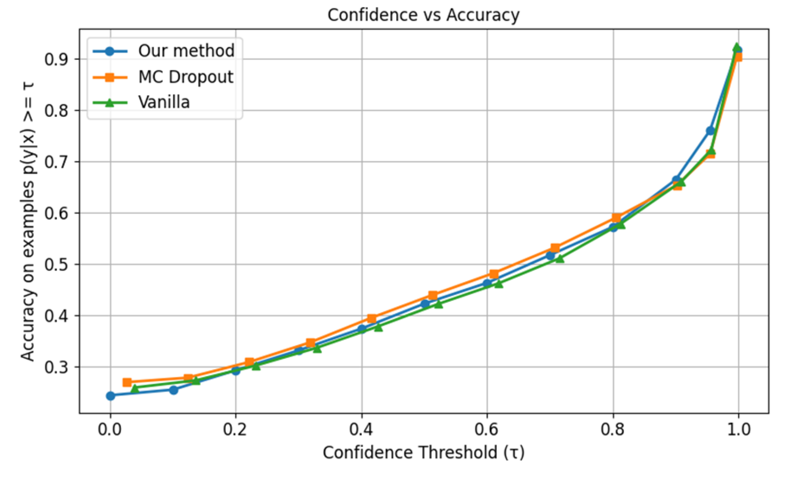
Figure 16.
ECE for level-3 distortion of Places365.

Figure 17.
Entropy for OOD samples using models trained with Places365.

Figure 18.
Confidence vs accuracy for original Places365 dataset for ensemble experiment.

Figure 19.
Confidence vs accuracy for Gussian-3 distortion of Places365 with ensemble approach.

Figure 20.
ECE for level-3 distortion of Places365 with ensemble approach.

Figure 21.
Entropy for OOD samples using models trained with Places365 with ensemble approach.


Table 1.
Metrics used in the experiments.
| Metric | Priority | Preference | Cal. steps |
|---|---|---|---|
| Acc. Vs Conf. | Primary | Problem dependent | All |
| ECE | Primary | ↓1 | All |
| BS | Secondary | ↓ | 1-3 |
| NLL | Secondary | ↓ | 1-3 |
| Entropy | Secondary | ↑ | 1-3 |
1 Symbol ↓ indicates lower is better, and ↑ indicates higher is better.
Table 2.
CIFAR-10 dataset.
| Item | Value |
|---|---|
| Training set | 50,000 |
| Test set | 10,000 |
| Image size | 32 × 32 pixels |
| Image channel | 3 (R, G, B) |
| No. of classes | 10 |
Table 3.
ImageNet 2012 dataset.
| Item | Value |
|---|---|
| Training set | 1,281,167 |
| Validation set | 50,000 |
| Test set | 100,000 (no label) |
| Image size | Variable (typically 224 × 224) |
| Image channel | 3 (R, G, B) |
| No. of classes | 1,000 |
Table 4.
iNaturalist 2018 dataset.
| Item | Value |
|---|---|
| Training set | 437,513 |
| Validation set | 24,426 |
| Test set | 149,394 (no label) |
| Image size | Variable (typically 224 × 224) |
| Image channel | 3 (R, G, B) |
| No. of classes | 8,142 |
| No. of super classes | 14 |
Table 5.
Places365 dataset.
| Item | Standard | Challenge |
|---|---|---|
| Training set | 1,800,000 | 8,000,000 |
| Validation set | 36,000 | 36,000 |
| Test set | 149,394 (no label) | |
| Image size | Variable, typically 224 × 224 or 256 × 256 | Variable, typically 224 × 224 or 256 × 256 |
| Image channel | 3 | 3 |
| No. of classes | 365 | 434 |
Table 6.
Distortion types used in the experiments.
| Category | Distortion |
|---|---|
| Blur | Glass blur, Defocus blur, Zoom blur, Gaussian blur |
| Noise | Impulse noise, Shot noise, Speckle noise, Gaussian noise |
| Transformation | Elastic transform, Pixelate |
| Color | Saturation, Brightness, Contrast |
| Environment | Fog, Spatter, Frost (not for iNaturalist2018 & Places365) |
Table 7.
Models used in experiments.
| Item | CIFAR-10 | ImageNet 2012 | iNaturalist 2018 | Places365 |
|---|---|---|---|---|
| Framework | TensorFlow | PyTorch | PyTorch | PyTorch |
| Structure | ResNet-20 V1 | ResNet-50 | ResNet-50 | VGG-16 |
| Training epochs | 200 | Pre-trained | 50 | Pre-trained |
| Batch size/Model | 7 | IMAGENET1K_V1 | 80 | CSAIL Vision |
| Optimizer | Adam | - | SGD | - |
| Learning rate | 0.000717 | - | 0.1 | - |
| Momentum | - | - | 0.9 | - |
| Loss | Categorical cross entropy | Categorical cross entropy | Categorical cross entropy | Categorical cross entropy |
Table 8.
Experimental parameters.
| Item | CIFAR-10 | ImageNet 2012 | iNaturalist 2018 | Places365 |
|---|---|---|---|---|
| Mask size | 3 × 3 | 20 × 20 | 20 × 20 | 20 × 20 |
| Hop size | 1 × 1 | 10 × 10 | 10 × 10 | 10 × 10 |
| in Eq. (2) | 1/2 | 1/2 | 1/2 | 1/2 |
| In-distribution image | 10,000 | 10,000 | 5,000 | 5,000 |
| Distorted image | 80,000 | 32,000 | 15,000 | 15,000 |
| OOD image | 26,032 | 1,000 | 1,000 | 1,000 |
Table 9.
Metrics for CIFAR-10 in-distribution dataset.
| Metrics | Proposed | MC dropout | Vanilla |
|---|---|---|---|
| Accuracy | 87.80% | ~91.2% | ~90.5% |
| ECE | 0.0693 | ~0.01 | ~0.05 |
| Brier Score | 0.2036 | ~0.13 | ~0.15 |
Table 10.
Metrics for original ImageNet 2012 dataset.
| Metrics | Proposed | MC dropout | Vanilla |
|---|---|---|---|
| Accuracy | 75.94% | ~74.55% | ~75.0% |
| ECE | 0.026 | ~0.015 | ~0.040 |
| Brier Score | 0.342 | ~0.35 | ~0.34 |
| NLL | 0.998 | ~1.1 | ~1.1 |
Table 11.
Metrics for original iNaturalist 2018 dataset.
| Metrics | Proposed | MC dropout | Vanilla |
|---|---|---|---|
| ECE | 0.055 | 0.070 | 0.007 |
| Brier Score | 0.053 | 0.101 | 0.048 |
| NLL | 0.109 | 0.196 | 0.104 |
Table 12.
Metrics for original Places365 dataset.
| Metrics | Proposed | MC dropout | Vanilla |
|---|---|---|---|
| ECE | 0.062 | 0.047 | 0.043 |
| Brier Score | 0.461 | 0.443 | 0.449 |
| NLL | 1.165 | 1.112 | 1.108 |
Table 13.
Metrics for original Places365 dataset for ensemble experiment.
| Metrics | Proposed | MC dropout | Vanilla | Ensemble |
|---|---|---|---|---|
| ECE | 0.062 | 0.047 | 0.043 | 0.079 |
Disclaimer/Publisher’s Note: The statements, opinions and data contained in all publications are solely those of the individual author(s) and contributor(s) and not of MDPI and/or the editor(s). MDPI and/or the editor(s) disclaim responsibility for any injury to people or property resulting from any ideas, methods, instructions or products referred to in the content. |
© 2025 by the authors. Licensee MDPI, Basel, Switzerland. This article is an open access article distributed under the terms and conditions of the Creative Commons Attribution (CC BY) license (http://creativecommons.org/licenses/by/4.0/).
Copyright: This open access article is published under a Creative Commons CC BY 4.0 license, which permit the free download, distribution, and reuse, provided that the author and preprint are cited in any reuse.


