Submitted:
12 August 2025
Posted:
14 August 2025
You are already at the latest version
Abstract
Automated optical inspection (AOI) of wood surfaces is critical for ensuring product quality in the furniture and manufacturing industries; however, existing defect detection systems often struggle to generalize across complex grain patterns and diverse defect types. This study proposes a wood grain defect recognition model employing a Gabor Convolutional Network (GCN) that integrates convolutional neural networks (CNNs) with Gabor filters. To systematically optimize the network’s architecture and improve both detection accuracy and computational efficiency, the Taguchi method is employed to tune key hyperparameters, including convolutional kernel size, filter number, and Gabor parameters (frequency, orientation, and phase offset). Additionally, image tiling and augmentation techniques are employed to effectively increase the training dataset, thereby enhancing the model’s stability and accuracy. Experiments conducted on the MVTec Anomaly Detection dataset (wood category) demonstrate that the Taguchi-optimized GCN achieves an accuracy of 98.92%, outperforming a baseline CNN by 2.73%. Results confirm that Taguchi-optimized GCNs enhance defect detection performance and computational efficiency, making them valuable for smart manufacturing.
Keywords:
convolutional neural network
; Gabor filter
; Taguchi method
; wood grain defect detection
1. Introduction
Defect detection on wood surfaces is a critical task in the furniture and woodworking industries, directly influencing product quality, customer satisfaction, and production efficiency. While most modern manufacturing lines have adopted automation in machining and finishing processes, visual quality inspection remains predominantly manual. Such human-dependent inspection is prone to inconsistencies, fatigue-induced errors, and reduced throughput, leading to both false acceptance (leakage) and false rejection (overkill) of products. The integration of automated optical inspection (AOI) systems into production lines offers a practicable path toward smart manufacturing, enabling real-time, objective, and rapid defect detection. Recent advances in artificial intelligence (AI), particularly deep learning (DL), have significantly improved image-based defect detection in various industrial domains [1,2]. However, despite the progress in generic defect detection, research on wood grain defect detection remains limited [3,4,5], primarily due to the complex texture patterns and wide variability in defect appearance.
Gabor functions are based on the sinusoidal plane wave with particular frequency and orientation, which characterizes the spatial frequency information of the image. A set of Gabor filters with a variety of frequencies and orientations can effectively extract invariant features from an image. Due to these capabilities, Gabor filters are widely employed in image processing applications, such as texture classification, image retrieval and wood defect detection [6]. Through multi-scale and multi-orientation design, Gabor filters effectively extract rich texture features, making them particularly valuable for wood defect detection. They can capture slight texture variations on wood surfaces, aiding in the identification of defect locations and types. However, relying solely on Gabor filters for feature extraction may not be sufficient to handle the complexity and diversity of wood defects. Since wood defects exhibit diverse characteristics, more advanced feature learning and recognition techniques are required for accurate detection. To overcome this limitation, integrating Gabor filters with deep learning techniques has proven to be a highly effective strategy [7,8,9].
Convolutional neural networks (CNNs) are a deep learning architecture that leverages multiple layers of convolution and pooling operations to efficiently extract hierarchical features from images. CNNs have demonstrated highly effectiveness for tasks such as image classification, object detection, and segmentation [2]. Gabor convolutional networks (GCNs) integrate Gabor filters into CNNs, leveraging both the local feature extraction capability of Gabor filters and the feature learning and classification abilities of CNNs. This integration enhances the robustness of learned features against variations in orientation and scale [8]. However, despite these advantages, GCNs suffer from a more complex network architecture. Thus, optimizing the network architecture to enhance GCN performance and computational efficiency has become a valuable research topic.
The Taguchi method, developed by Dr. Genichi Taguchi, is a quality engineering approach primarily used for product design and process optimization. It employs design of experiments (DOE), particularly orthogonal arrays (OAs), to efficiently evaluate multiple factors affecting quality. Additionally, it incorporates the signal-to-noise (S/N) ratio to measure system robustness with the goal of reducing variation and improving product reliability. In addition, the Taguchi method offers the following advantages: (i) Reduced experimental cost and time – By leveraging orthogonal arrays, the method significantly reduces the number of experimental runs while still achieving optimal design parameters. (ii) Systematic problem-solving approach – Through parameter design and tolerance design, the method optimizes product performance during the development phase, thereby minimizing the need for costly modifications. Due to these benefits, the Taguchi method has been widely adopted in industries such as manufacturing, electronics, biomedical engineering, automotive, and semiconductor [10,11].
Generally speaking, the design of CNN and GCN involves numerous hyperparameters, such as convolutional kernel size, Gabor convolutional filters, pooling strategies, number of layers, and learning rate. Traditional hyperparameter optimization methods such as grid search and random search suffer from high computational costs and may fail to capture robust parameter settings under small-sample conditions. In contrast, the Taguchi method utilizes orthogonal arrays to efficiently select representative parameter sets, significantly reducing the number of experimental runs and computational costs. This advantage motivates the adoption of the Taguchi method for CNN and GCN optimization, as it not only reduces the computational burden of hyperparameter tuning but also enhances model robustness, convergence speed, and generalization ability. Furthermore, the Taguchi method is particularly well-suited for applications with limited data and computational resources, such as texture image analysis, industrial inspection, and intelligent surveillance systems. Therefore, it provides a highly efficient and systematic approach for optimizing CNN and GCN architectures.
Based on the aforementioned reasons and advantages, this study proposes a wood grain defect recognition model based on Gabor convolutional networks, integrating convolutional neural networks, Gabor filters, and the Taguchi method. The proposed GCN model employs the Taguchi method to optimize the network architecture. Furthermore, to address the issue of limited training samples, this study utilizes image tiling and data augmentation techniques to effectively increase the number of training samples, thereby enhancing the stability and accuracy of the model.
This study addresses these gaps by proposing a Taguchi-optimized Gabor convolutional network for wood grain defect detection. The main contributions of this work are as follows:
i) Integration of interpretable texture feature extraction and deep feature learning through a GCN architecture specifically adapted for wood surface inspection.
ii) Systematic optimization of GCN hyperparameters using the Taguchi method, enabling high performance with reduced computational cost.
iii) Data augmentation and tiling strategies to overcome limited training data, enhancing model stability and generalization.
iv) Extensive comparative evaluation against a baseline CNN on the MVTec AD wood category dataset, demonstrating a 2.73% accuracy improvement.
The remainder of this study is organized as follows. Section 2 briefly reviews some studies on Gabor filters, CNNs, and their combination. The proposed optimization of Gabor convolutional networks using the Taguchi method and their application in wood grain defect detection are given in Section 3. Finally, Section 4 presents some conclusions of this study.
2. Literature Review
2.1. Gabor Filters
Gabor filters are widely recognized for their effectiveness in extracting spatial frequency and orientation information from images. A two-dimensional Gabor function can be formulated as a Gaussian kernel modulated by a sinusoidal plane wave, enabling multi-scale and multi-orientation analysis [6]. The two-dimensional (2D) Gabor function, represented as a Gaussian kernel function modulated by a sinusoidal plane wave, is defined as follows.
where
where x and y are the Cartesian coordinates, represents the frequency, denotes the orientation, corresponds to the bandwidth (the standard deviation of the Gaussian function), indicates the phase offset, and refers to the spatial aspect ratio. A set of Gabor filters with a variety of frequencies and orientations can extract invariant features from an image. Hence, the Gabor filters are widely used in the field of image processing, such as texture classification and retrieval. This property makes Gabor filters particularly suitable for texture analysis tasks, including texture classification, content-based image retrieval, and industrial surface inspection [7,8,9].
In the context of wood surface inspection, Gabor filters can capture subtle variations in grain patterns, facilitating the identification of defects such as scratches, discolorations, or holes. However, their handcrafted nature imposes limitations: the extracted features are fixed once the filter bank is designed, making them less adaptive to variations in illumination, defect shape, or environmental noise. Furthermore, when applied in isolation, Gabor-based methods often struggle with complex intra-class variability, leading to reduced robustness in unconstrained industrial settings.
2.2. Convolutional Neural Networks
In the field of machine vision, convolutional neural networks are the most widely used deep learning architecture, such as the LeNet-5 architecture shown in Figure 1 [12]. This architecture comprises three primary types of neural layers: convolutional layers, pooling layers, and fully connected layers. The convolutional layers are responsible for extracting local features from images, while the pooling layers reduce image dimensions and network parameters. The fully connected layers transform the two-dimensional image representation into a one-dimensional vector. Finally, the output layer, utilizing the Softmax function as the activation function, determines the network’s final prediction by selecting the neuron with the highest activation.
Nonetheless, conventional CNN kernels are learned from data without explicit constraints on their frequency or orientation selectivity. While this flexibility can be advantageous in learning task-specific features, it may result in redundancy or suboptimal exploitation of structural priors in texture-rich domains such as wood surfaces. This limitation motivates the incorporation of domain-specific filters, such as Gabor filters, into CNN architectures to improve orientation-sensitive feature representation.
2.3. Integrating Gabor Filters with CNN Architectures
The integration of Gabor filters into CNNs has been investigated to combine the interpretable, orientation-sensitive feature extraction of Gabor filters with the deep, hierarchical feature learning capabilities of CNNs. Existing approaches can be broadly categorized into two strategies:
i) Pre-processing-based integration – Gabor filters are first applied to raw images to generate feature maps, which are then fed into a CNN for further processing [9,13,14]. This approach enhances the input representation but does not alter the CNN architecture.
ii) Kernel-substitution integration – Conventional convolutional kernels in the CNN are replaced with Gabor kernels, either fixed or learnable, enabling the network to perform Gabor-based filtering in its early layers [8,15,16]. This strategy embeds prior knowledge directly into the architecture, often improving robustness to variations in orientation and scale.
Empirical studies have demonstrated that Gabor-augmented CNNs (GCNs) can outperform conventional CNNs in tasks involving fine-grained textures, such as natural image classification task (CIFAR datasets) [8], small-sample object detection [9], and print defect detection [14]. However, most prior work has relied on heuristic or trial-and-error tuning of Gabor parameters (e.g., frequency, orientation, phase offset) and CNN hyperparameters (e.g., kernel size, number of filters), which can be computationally expensive and may not yield globally optimal configurations.
2.4. Parameter Optimization in Deep Learning Using the Taguchi Method
The Taguchi method is a robust design optimization approach that utilizes orthogonal arrays and signal-to-noise (S/N) ratio analysis to identify optimal parameter configurations with a minimal number of experiments [10,11]. Originally developed for manufacturing process optimization, it has been successfully applied to domains such as electronics, biomedical engineering, and industrial quality control. In the context of deep learning, the Taguchi method offers a computationally efficient alternative to exhaustive hyperparameter searches, especially for scenarios with limited training data and resources.
Despite its advantages, the application of the Taguchi method to optimize deep learning architectures—particularly Gabor-based CNNs—remains underexplored. This represents a significant opportunity to systematically determine both Gabor filter parameters and CNN architectural hyperparameters, potentially leading to performance gains without incurring prohibitive computational costs.
3. Proposed Methodology
The architecture of Gabor convolutional network (GCN) is illustrated in Figure 2. This design builds upon the foundational LeNet-5 architecture, as depicted in Figure 1. Notably, in the GCN architecture, the initial layer is a convolutional layer that employs Gabor kernels [17]. This modification preserves the filtering and feature extraction capabilities inherent to traditional convolutional layers. Additionally, it offers advantages such as reducing the need for extensive data preprocessing and enhancing the computational efficiency of the network.
This study utilizes the wood category from the MVTec Anomaly Detection (MVTec AD) dataset [18]. The MVTec AD dataset comprises 15 categories with 3,629 images for training and validation and 1,725 images for testing. The training set contains only images without defects. The test set contains both: images containing various types of defects and defect-free images. Within this dataset, the wood category includes images of defects such as color anomalies, holes, liquid, and scratch, as illustrated in Figure 3. Table 1 presents the number of images for each type within the wood category, where “Good” represents defect-free. Note that MVTec AD dataset includes 247 defect-free images for training and validation and 19 images for testing. Therefore, the total number of defect-free images, as represented in the "Good" category (second row of the table), is 266.
In the experimental setup, the model-building environment utilized Pytorch 2.3.0, Jupyter Notebook 7.0.6, and TensorFlow 2.10.0. The test environment comprised an Intel(R) Core™ i7-13700H CPU @ 3.40 GHz processor, 32.0 GB of RAM, an Nvidia GeForce RTX 3060 Ti GPU, and a Windows 11 64-bit operating system.
3.1. Data Preprocessing
Due to the lack of training samples for wood defect detection, this study employs two approaches to increase the number of training samples and reduce computational load:
i) Image tiling: The original wood grain images are divided into smaller tiles to increase the number of defect samples while simultaneously reducing computational complexity. In this study, a 1024×1024-pixel image is tiled into 64 sub-images of 128×128 pixels. Furthermore, when the tiled images serve as input to the defect detection model, if a specific sub-image is classified as a certain defect category, the corresponding region in the original image can be marked as the defect location. This enables both defect classification and localization within wood grain images.
ii)Image augmentation: To enhance the diversity of training samples and expand the dataset, this study applies various image augmentation techniques, including rotation, horizontal translation, vertical translation, and random scaling.
After applying the aforementioned two data preprocessing methods, the training dataset for this study consists of a total of 10,000 samples (2,000 per category), while the test dataset contains 2,000 samples (400 per category), as shown in Table 1. During the training process, 80% of the training samples are used for model training to optimize the model parameters, while the remaining 20% serve as the validation set to evaluate the model’s confirm the optimal configuration performance.
3.2. Steps for Implementing the Taguchi Method
The Taguchi method is a systematic approach for optimizing process parameters by minimizing variability and improving robustness. It employs a structured experimental design using orthogonal arrays (OAs) to efficiently determine the optimal factor levels [10,11]. The following steps outline its implementation in optimizing a GCN or CNN for wood grain defect detection.
i) Define the problem and objective: The first step involves identifying the need for optimization, such as improving the accuracy of wood grain defect detection using a GCN or CNN. To achieve this, it is crucial to determine the key factors influencing model performance. These factors include convolutional kernel size, the number of filters, and Gabor filter properties like frequency, orientation, and phase offset.
ii) Select control factors and levels: After defining the problem, the next step is to choose the parameters (control factors) that will be optimized and assign appropriate levels to each. For instance, convolutional kernel size may have three levels: 3×3, 5×5, and 7×7, while the number of filters in different layers may vary across experiments. Proper selection of these factors ensures that the experimental design captures a wide range of potential improvements.
iii) Design the experiment using an orthogonal array: Instead of testing all possible combinations, which would be computationally expensive, an orthogonal array (OA) is selected to systematically conduct experiments with reduced trials. The OA helps distribute experiments evenly across factor levels, ensuring a balanced analysis.
iv) Conduct experiments and record performance: Each experimental configuration is implemented by training and testing the GCN or CNN under the selected parameter settings.
v) Calculate the signal-to-noise (S/N) ratio: To measure the robustness of each configuration, the signal-to-noise (S/N) ratio is calculated.
vi) Analyze results and determine optimal factor levels: Once the S/N ratios are computed, the average S/N ratio for each factor level is analyzed to determine the optimal combination. The best parameter settings are selected based on the highest S/N ratios, and response plots are generated to visualize their effects on model performance.
vii) Confirm the optimal configuration: The GCN is then retrained using the optimized parameters to validate its performance. A comparison with a baseline CNN is conducted to assess improvements in accuracy and computational efficiency. The results confirm whether the optimized model outperforms the traditional approach.
viii) Implement and verify performance: Finally, the optimized model is applied to real-world wood defect detection tasks. Further evaluations are conducted to ensure its robustness and generalization ability. If needed, additional refinements can be made to enhance the model’s effectiveness.
3.3. Optimizing Gabor Convolutional Networks Using the Taguchi Method
This study employs the Taguchi method to optimize the architecture of the Gabor convolutional network. The control factors to be optimized, along with their corresponding levels, are shown in Table 2. Among these, three control factors—frequency (ω), orientation (θ), and phase offset (ψ)—are related to the Gabor filter parameters, while the remaining five control factors are hyperparameters associated with the convolutional layers. As shown in Table 2, there is one factor with two levels and seven factors with three levels, resulting in a total of 15 degrees of freedom for the eight control factors. Consequently, an orthogonal array with at least 15 degrees of freedom is required for the Taguchi experiment. In this study, the L18 (2¹×3⁷) orthogonal array, as listed in Table 3, is selected, requiring 18 experimental runs to systematically evaluate the factor-level combinations. Without the orthogonal array, a total of 4,374 (2¹×3⁷) experiments would be required. However, by applying the orthogonal array, only 18 experiments are needed in this study.
To reduce the influence of randomness and enhance reliability, each experimental configuration is independently executed 10 times. The average accuracy for each independent trial is recorded, and the mean of these 10 trials is used to represent the experimental performance of that configuration, as shown in Table 4. For convenience, the average accuracy is also included in the aforementioned Table 3. A higher mean value indicates a higher average accuracy for that configuration. Since the objective of applying the Taguchi method is to improve the recognition accuracy of the Gabor convolutional network, this study considers the “larger-the-better” quality characteristic. Therefore, the “larger-the-better” formulation of the Taguchi method is applied for the calculation of the signal-to-noise (S/N) ratio, as expressed in Eq. 4:
where represents the ith observed value, and n denotes the total number of observations.
Based on the L18 orthogonal array and the recognition results of Table 4 (at the end of the paper), the S/N ratio for each experimental setup is listed in the last column of Table 3. The average S/N ratio of each factor and level is listed in Table 5. The higher S/N ratio represents the higher stability of the quality. The optimal parameter of each factor is also displayed in the last row in Table 5. Figure 4 presents the factor S/N ratio response plot, which illustrates the mean response values calculated for each control factor and its corresponding levels. Since the quality characteristic of this study follows the “larger-the-better” criterion, the optimal factor settings can be identified from the response plot in Figure 4 as follows: the pooling method is max pooling, the number of filters in the first convolutional layer is 256, the kernel size of the first convolutional layer is (7,7), the number of filters in the second convolutional layer is 128, the kernel size of the second convolutional layer is (3,3), the number of frequency components is 6, the number of orientations is 4, and the number of phase offsets is 3.
3.4. Optimizing Convolutional Neural Networks Using the Taguchi Method
In this study, the control group employs a traditional convolutional neural network (CNN) with an architecture similar to the Gabor convolutional network shown in Figure 2. This network comprises two convolutional layers with corresponding pooling layers, followed by two fully connected layers. To optimize the CNN’s hyperparameters, the Taguchi method is applied, focusing on control factors and levels. The control factors and their corresponding levels are listed in Table 6, while Table 7 presents the L8 orthogonal array used in this study. The experimental results and S/N ratios are provided in Table 8 and the last column of Table 7, respectively.
The average S/N ratio of each factor and level, along with the optimal parameter of each factor, is presented in Table 5. Additionally, Figure 5 depicts the corresponding Taguchi response plot, which illustrates the mean response values calculated for each control factor and its associated levels. Based on these results, the optimized control factors for the CNN are identified as follows: the pooling method is max pooling, the number of filters in the first convolutional layer is 128, the kernel size of the first convolutional layer is (3,3), the pooling size of the first pooling layer is 4, the number of filters in the second convolutional layer is 128, the kernel size of the second convolutional layer is (3,3), and the pooling size of the second pooling layer is 2.

Table 6.
Levels of control factors: CNNs.
| No. | Control Factors | Level 1 | Level 2 |
| A | Pooling function | Max | Average |
| B | Conv1_filters | 128 | 512 |
| C | Conv1_kernel size | (3,3) | (7,7) |
| D | Conv1_pool_size | 2 | 4 |
| E | Conv2_filters | 128 | 512 |
| F | Conv2_kernel size | (3,3) | (7,7) |
| G | Conv2_pool_size | 2 | 4 |
Table 7.
average accuracy and S/N ratio of L8 orthogonal array: CNNs.
| No. | A | B | C | D | E | F | G | Ave. Acc. | S/N |
| 1 | 1 | 1 | 1 | 1 | 1 | 1 | 1 | 95.94% | -0.3654 |
| 2 | 1 | 1 | 1 | 2 | 2 | 2 | 2 | 98.22% | -0.1568 |
| 3 | 1 | 2 | 2 | 1 | 1 | 2 | 2 | 92.65% | -0.7590 |
| 4 | 1 | 2 | 2 | 2 | 2 | 1 | 1 | 96.38% | -0.3233 |
| 5 | 2 | 1 | 2 | 1 | 2 | 1 | 2 | 92.33% | -0.7243 |
| 6 | 2 | 1 | 2 | 2 | 1 | 2 | 1 | 96.15% | -0.3465 |
| 7 | 2 | 2 | 1 | 1 | 2 | 2 | 1 | 91.82% | -0.7503 |
| 8 | 2 | 2 | 1 | 2 | 1 | 1 | 2 | 97.95% | -0.1805 |
Table 8.
Recognition accuracy of convolutional neural networks.
| Exp. | Run 1 | Run 2 | Run 3 | Run 4 | Run 5 | Run 6 | Run 7 | Run 8 | Run 9 | Run 10 | Average |
| 1 | 93.60% | 97.65% | 95.60% | 96.75% | 98.05% | 99.15% | 94.76% | 97.00% | 93.02% | 93.85% | 95.94% |
| 2 | 98.85% | 96.80% | 98.40% | 98.75% | 98.85% | 97.03% | 98.21% | 99.12% | 98.26% | 97.93% | 98.22% |
| 3 | 97.50% | 79.90% | 96.40% | 97.65% | 98.20% | 91.97% | 97.23% | 93.78% | 96.81% | 77.03% | 92.65% |
| 4 | 93.70% | 97.45% | 94.10% | 98.00% | 97.90% | 96.24% | 95.95% | 97.05% | 97.65% | 95.76% | 96.38% |
| 5 | 97.40% | 95.50% | 86.15% | 97.65% | 91.00% | 87.99% | 87.83% | 92.28% | 99.08% | 88.39% | 92.33% |
| 6 | 93.85% | 96.80% | 92.45% | 96.80% | 96.35% | 98.13% | 94.85% | 95.69% | 98.69% | 97.85% | 96.15% |
| 7 | 89.65% | 95.75% | 87.60% | 91.15% | 92.65% | 91.64% | 90.87% | 90.83% | 96.27% | 91.82% | 91.82% |
| 8 | 97.90% | 98.15% | 97.10% | 98.65% | 98.45% | 97.04% | 98.71% | 97.31% | 97.83% | 98.35% | 97.95% |
Table 9.
Factor S/N Ratio Response Table: CNNs.
| Level | A | B | C | D | E | F | G |
| 1 | -0.4011 | -0.3982 | -0.3632 | -0.6498 | -0.4128 | -0.3984 | -0.4464 |
| 2 | -0.5004 | -0.5033 | -0.5383 | -0.2518 | -0.4887 | -0.5031 | -0.4552 |
| rank | 5 | 3 | 2 | 1 | 6 | 4 | 7 |
| best | Max | 128 | (3,3) | 4 | 128 | (3,3) | 2 |
3.5. Comparative Analysis of Optimal Factor Combinations
The final experiment is performed based on the optimal factor combination. To ensure the reliability and stability of the results, the optimized Gabor convolutional network and the optimized convolutional neural network were independently executed ten times each, with the average accuracy serving as the primary metric for evaluating their predictive performance. The experimental results and corresponding average values are presented in Table 10. The optimized GCN achieved an average accuracy of 98.92%, whereas the optimized CNN attained 96.19%.
These findings demonstrate that the optimized GCN outperforms the optimized CNN by 2.73% in wood grain defect detection. This improvement can be attributed to the integration of the Gabor filter with the CNN architecture, which enhances the model's ability to extract texture features more effectively. By leveraging the superior edge and texture detection capabilities of the Gabor filter, the GCN not only achieves higher detection accuracy but also exhibits greater robustness and reliability in defect detection tasks.
4. Conclusions
This study presented a Taguchi-optimized Gabor Convolutional Network for wood grain defect detection, integrating the orientation- and frequency-selective texture analysis of Gabor filters with the hierarchical feature learning of convolutional neural networks (CNNs). The Taguchi method was employed to systematically tune both CNN architectural parameters and Gabor-specific settings, enabling performance optimization with a substantially reduced number of experimental trials compared to exhaustive search. To address the challenge of limited training data, an image tiling and augmentation pipeline was introduced, expanding the dataset and improving model generalization.
Experimental evaluation on the MVTec Anomaly Detection dataset (wood category) demonstrated that the optimized GCN achieved an average detection accuracy of 98.92%, outperforming a Taguchi-optimized baseline CNN by 2.73%. This improvement confirms the effectiveness of combining interpretable, domain-specific feature extraction with statistical design-of-experiments in developing lightweight yet accurate defect detection models suitable for real-time smart manufacturing applications.
Acknowledgments
This work was supported by National Science and Technology Council, Taiwan through Grant NSTC 112-2637-E-262-005 and MTSC 113-2637-E-262-001.
References
- M. Mohsin, et al., “Real-time defect detection and classification on wood surfaces using deep learning,” Proc. IS&T Int. Symp. Electron. Imaging, New York, NY, USA, pp. 381-1–382-6, 2022. [CrossRef]
- W. Lu, J. F. W. Lu, J. F. Jing, and Y. Q. Huang, “MRD-Net: An effective CNN-based segmentation network for surface defect detection,” IEEE Trans. Instrum. Meas., vol. 71, no. 2516812, 2022. [CrossRef]
- Mazhar Mohsin, et al, “Real-time defect detection and classification on wood surfaces using deep learning,” Proc. IS&T International Symposium on Electronic Imaging, New York, USA, pp. 381-1~382-6, 2022. [CrossRef]
- D. J. Li, W. B. D. J. Li, W. B. Xie, B. G. Wang, W. F. Zhong, and H. M. Wang, “Data augmentation and layered deformable Mask R-CNN-based detection of wood defects,” Proc. IEEE, vol. 9, pp. 108162-108174, 2021. [CrossRef]
- S.-W. Hwang and J. Sugiyama, “Computer vision-based wood identification and its expansion and contribution potentials in wood science: A review,” Plant Methods, 17: 47, 2021. [CrossRef]
- J. Han and K.-K. Ma, “Rotation-invariant and scale-invariant Gabor features for texture image retrieval,” Image Vis. Comput., vol. 25, no. 9, pp. 1474–1481, 2007. [CrossRef]
- Y. Yuan, L.-N. Y. Yuan, L.-N. Wang, G.-Q. Zhong, W. Ga, W.-C. Jiao, J.-Y. Dong, B. Shen, D.-D. Xia, and W. Xiang, “Adaptive Gabor convolutional networks,” Pattern Recognit., vol. 124, no. 108495, 2022. [CrossRef]
- S. Luan, C. S. Luan, C. Chen, B. Zhang, J. Han, and J. Liu, “Gabor convolutional networks,” IEEE Trans. Image Process., vol. 27, no. 9, pp. 4357–4366, 2018.
- X.-D. Hu, et al., “Gabor-CNN for object detection based on small samples,” Defence Technol., vol. 16, no. 6, pp. 1116–1129, 2020. [CrossRef]
- G. Taguchi, Introduction to Quality Engineering: Designing Quality into Products and Processes, Tokyo, Japan: Asian Productivity Organization, 1986. [CrossRef]
- R. Kacker, T. R. Kacker, T. Lagergren, and B. L. Gu, “Taguchi’s orthogonal arrays are classical designs of experiments,” J. Res. Natl. Inst. Stand. Technol., vol. 96, no. 5, p. 577, Sep. 1991. [CrossRef]
- Y. LeCun, L. Y. LeCun, L. Bottou, Y. Bengio, and P. Haffner, “Gradient-based learning applied to document recognition,” Proc. IEEE, vol. 86, no. 11, pp. 2278–2324, 1998. [CrossRef]
- H. Yao, et al., “Gabor feature based convolutional neural network for object recognition in natural scene,” Proc. 2016 3rd ICISCE, Beijing, China, pp. 386-390, 2016.
- S. Wang, et al., “Detection of overprint defects by PSO-Gabor-CNN algorithms,” Packaging Engineering, vol. 41, no. 5, pp. 214-222, 2020.
- S. S. Sarwar, P. Panda and K. Roy, “Gabor filter assisted energy efficient fast learning convolutional neural networks,” Proc. 2017 IEEE/ACM ISLPED, Taipei, Taiwan, 2017 (arXiv:1705.04748v1).
- F. Meng, et al., “Energy-efficient Gabor kernels in neural networks with genetic algorithm training method,” Electronics, vol. 8, no. 1, 105, 2019. [CrossRef]
- Alekseev and A. Bobe, “GaborNet: Gabor filters with learnable parameters in deep convolutional neural networks,” arXiv preprint arXiv:1904.13204, 2019.
- P. Bergmann, M. P. Bergmann, M. Fauser, D. Sattlegger, and C. Steger, "MVTec AD—A comprehensive real-world dataset for unsupervised anomaly detection," in Proc. IEEE/CVF Conf. Comput. Vis. Pattern Recognit. (CVPR), 2019, pp. 9592–9600.
Figure 1.
Architecture of LeNet-5 [12].
Figure 1.
Architecture of LeNet-5 [12].
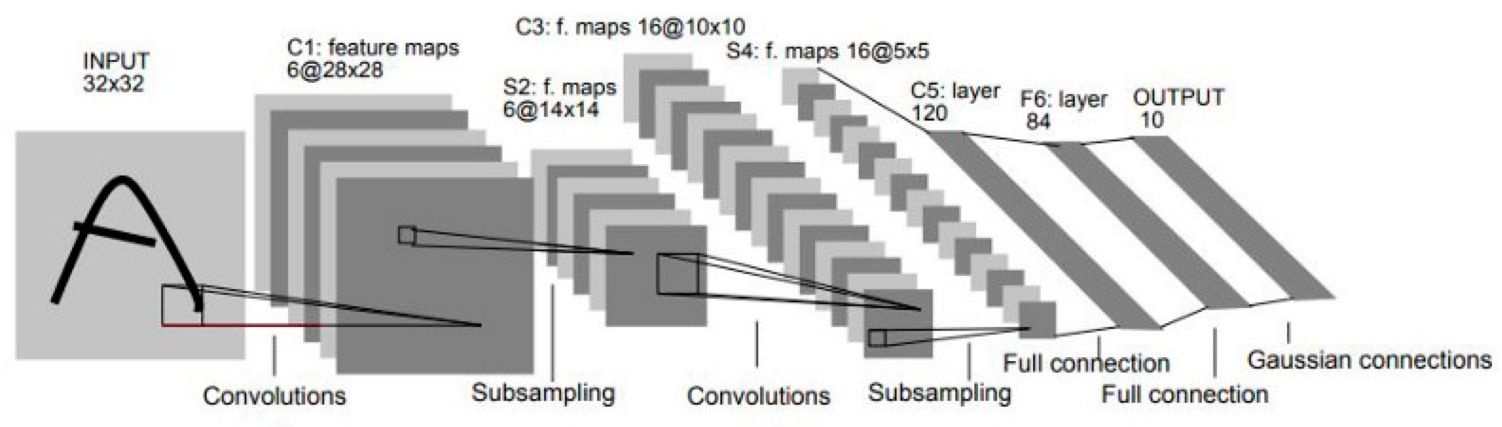
Figure 2.
Architecture of Gabor convolutional networks.
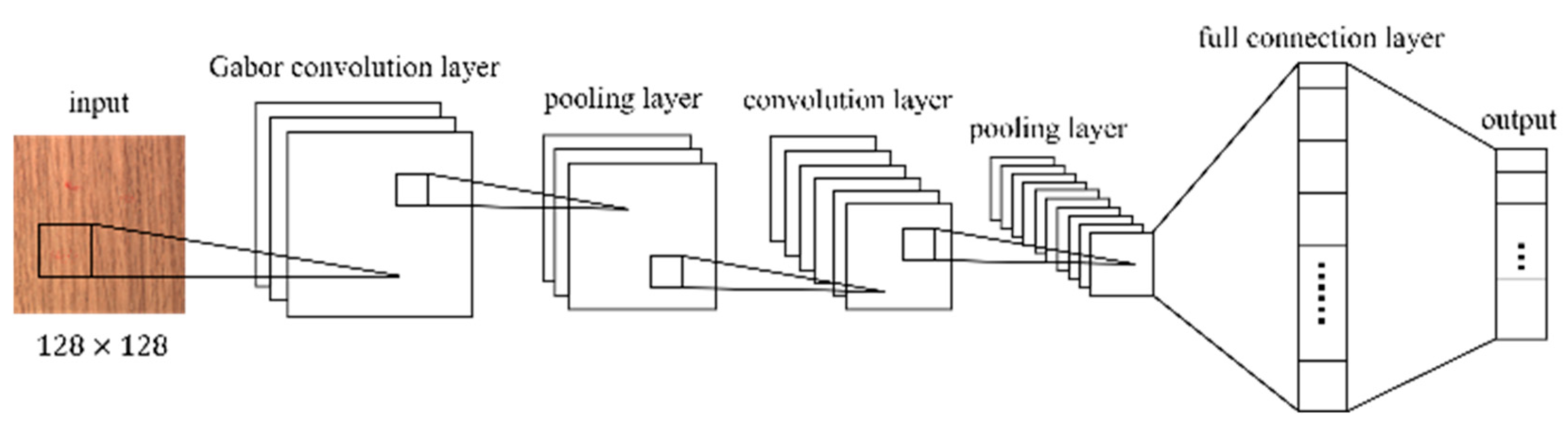
Figure 3.
Types of good and defective wood grain patterns.
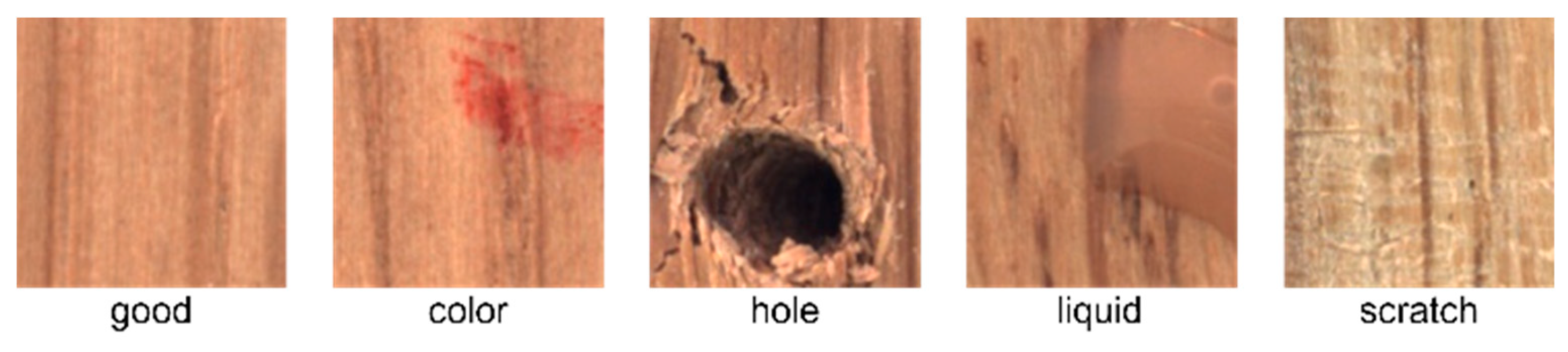
Figure 4.
Factor S/N ratio response plot: Gabor convolutional networks.
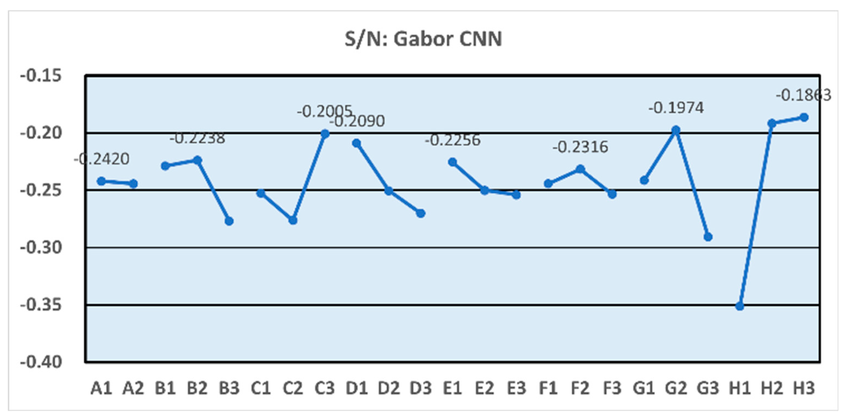
Figure 5.
Factor S/N ratio response plot: Convolutional neural networks.
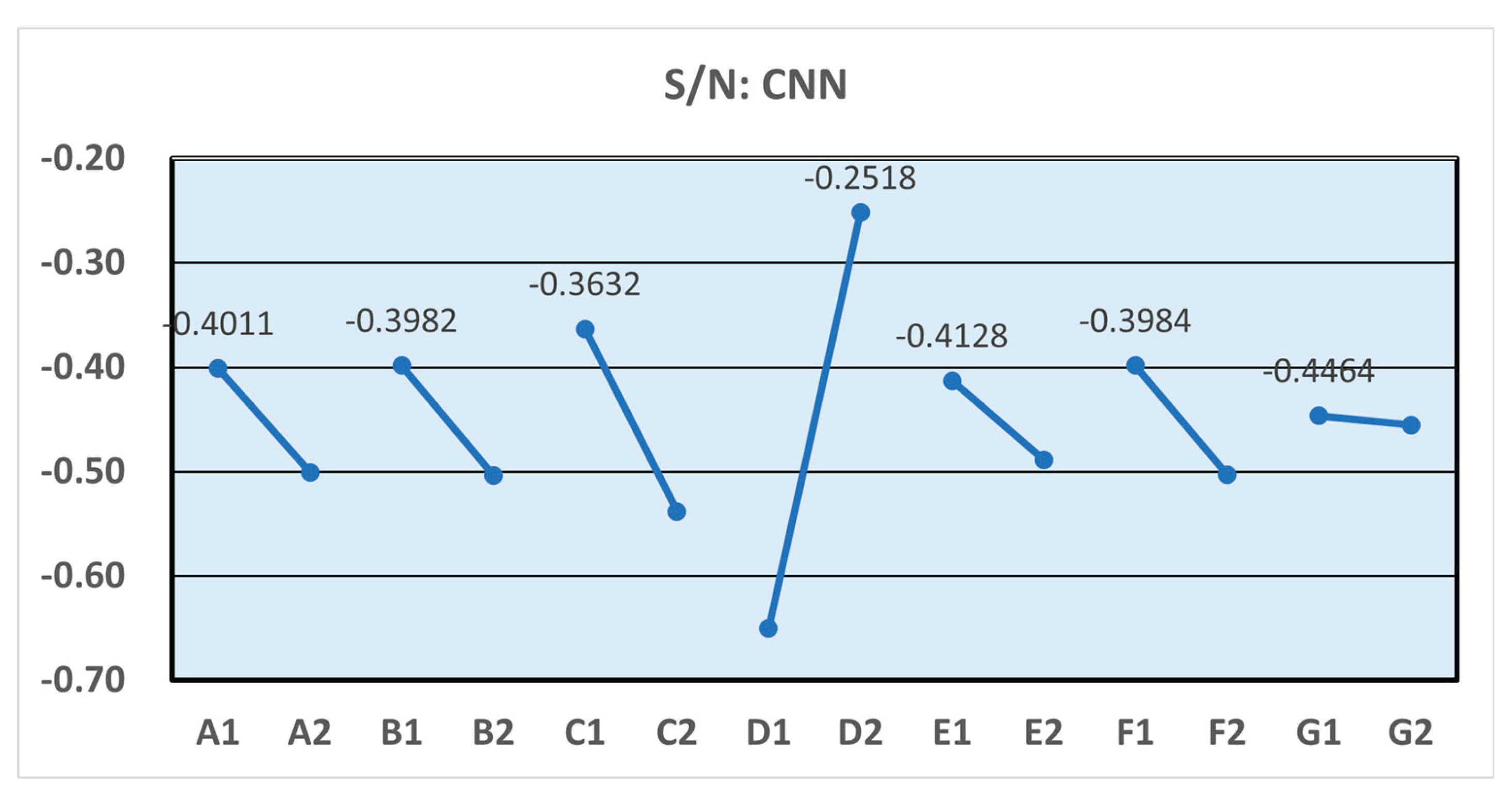
Table 1.
Number of images for each type in wood category.
| Type | Good | Color | Hole | Liquid | Scratch | Total |
| MVTec | 266 | 8 | 10 | 10 | 21 | 315 |
| Train | 2,000 | 2,000 | 2,000 | 2,000 | 2,000 | 10,000 |
| Test | 400 | 400 | 400 | 400 | 400 | 2,000 |
Table 2.
Levels of control factors: GCNs.
| No. | Control Factors | Level 1 | Level 2 | Level 3 |
| A | Pooling function | Max | Average | --- |
| B | Conv1_filters | 128 | 256 | 512 |
| C | Conv1_kernel size | (3,3) | (5,5) | (7,7) |
| D | Conv2_filters | 128 | 256 | 512 |
| E | Conv2_kernel size | (3,3) | (5,5) | (7,7) |
| F | frequency ω | 5 | 6 | 7 |
| G | orientation θ | 2 | 4 | 6 |
| H | phase offset ψ | 1 | 2 | 3 |
Table 3.
average accuracy and S/N ratio of L18 orthogonal array: GCNs.
| No. | A | B | C | D | E | F | G | H | Ave. Acc. | S/N |
| 1 | 1 | 1 | 1 | 1 | 1 | 1 | 1 | 1 | 97.01% | -0.2635 |
| 2 | 1 | 1 | 2 | 2 | 2 | 2 | 2 | 2 | 98.45% | -0.1366 |
| 3 | 1 | 1 | 3 | 3 | 3 | 3 | 3 | 3 | 97.83% | -0.1939 |
| 4 | 1 | 2 | 1 | 1 | 2 | 2 | 3 | 3 | 97.75% | -0.1990 |
| 5 | 1 | 2 | 2 | 2 | 3 | 3 | 1 | 1 | 95.50% | -0.4058 |
| 6 | 1 | 2 | 3 | 3 | 1 | 1 | 2 | 2 | 98.77% | -0.1083 |
| 7 | 1 | 3 | 1 | 2 | 1 | 3 | 2 | 3 | 97.75% | -0.1973 |
| 8 | 1 | 3 | 2 | 3 | 2 | 1 | 3 | 1 | 94.43% | -0.5143 |
| 9 | 1 | 3 | 3 | 1 | 3 | 2 | 1 | 2 | 98.19% | -0.1595 |
| 10 | 2 | 1 | 1 | 3 | 3 | 2 | 2 | 1 | 95.97% | -0.3579 |
| 11 | 2 | 1 | 2 | 1 | 1 | 3 | 3 | 2 | 97.20% | -0.2477 |
| 12 | 2 | 1 | 3 | 2 | 2 | 1 | 1 | 3 | 98.02% | -0.1739 |
| 13 | 2 | 2 | 1 | 2 | 3 | 1 | 3 | 2 | 97.37% | -0.2346 |
| 14 | 2 | 2 | 2 | 3 | 1 | 2 | 1 | 3 | 97.93% | -0.1821 |
| 15 | 2 | 2 | 3 | 1 | 2 | 3 | 2 | 1 | 97.59% | -0.2129 |
| 16 | 2 | 3 | 1 | 3 | 2 | 3 | 1 | 2 | 97.05% | -0.2633 |
| 17 | 2 | 3 | 2 | 1 | 3 | 1 | 2 | 3 | 98.05% | -0.1716 |
| 18 | 2 | 3 | 3 | 2 | 1 | 2 | 3 | 1 | 96.06% | -0.3547 |
Table 4.
Recognition results of Gabor convolutional networks.
| Exp. | Run 1 | Run 2 | Run 3 | Run 4 | Run 5 | Run 6 | Run 7 | Run 8 | Run 9 | Run 10 | Average |
| 1 | 96.75% | 97.25% | 96.80% | 96.55% | 96.90% | 97.14% | 97.33% | 96.67% | 97.63% | 97.13% | 97.01% |
| 2 | 98.75% | 99.05% | 99.05% | 97.35% | 98.50% | 99.13% | 98.01% | 97.58% | 98.65% | 98.38% | 98.45% |
| 3 | 98.80% | 95.20% | 95.75% | 98.90% | 97.80% | 98.78% | 100.57% | 96.45% | 98.68% | 97.37% | 97.83% |
| 4 | 97.95% | 97.30% | 98.95% | 96.65% | 98.70% | 97.30% | 97.58% | 97.24% | 96.63% | 99.15% | 97.75% |
| 5 | 96.65% | 91.95% | 95.25% | 97.60% | 97.30% | 96.29% | 94.15% | 98.23% | 92.45% | 95.14% | 95.50% |
| 6 | 99.15% | 99.15% | 98.70% | 97.90% | 99.00% | 97.48% | 98.78% | 99.05% | 99.12% | 99.33% | 98.77% |
| 7 | 98.10% | 97.55% | 97.85% | 97.85% | 97.65% | 97.76% | 97.85% | 97.64% | 97.56% | 97.74% | 97.75% |
| 8 | 96.80% | 88.75% | 98.15% | 90.70% | 96.65% | 99.14% | 96.48% | 92.03% | 93.94% | 91.64% | 94.43% |
| 9 | 96.55% | 99.20% | 97.50% | 99.35% | 98.10% | 97.96% | 98.76% | 97.75% | 99.01% | 97.72% | 98.19% |
| 10 | 95.60% | 97.00% | 95.20% | 96.00% | 96.45% | 94.70% | 95.47% | 96.49% | 96.89% | 95.92% | 95.97% |
| 11 | 97.75% | 98.80% | 97.55% | 96.50% | 96.70% | 97.72% | 97.34% | 95.78% | 97.51% | 96.34% | 97.20% |
| 12 | 98.25% | 98.50% | 97.60% | 98.85% | 97.65% | 98.24% | 98.94% | 96.89% | 97.15% | 98.16% | 98.02% |
| 13 | 98.70% | 97.45% | 99.05% | 94.65% | 98.65% | 95.71% | 98.38% | 98.88% | 96.42% | 95.81% | 97.37% |
| 14 | 97.80% | 96.50% | 98.40% | 98.15% | 98.30% | 98.70% | 97.41% | 98.11% | 98.71% | 97.24% | 97.93% |
| 15 | 97.35% | 95.85% | 98.45% | 96.85% | 98.25% | 97.32% | 98.92% | 97.80% | 96.66% | 98.45% | 97.59% |
| 16 | 98.15% | 95.85% | 97.95% | 98.30% | 93.70% | 98.83% | 95.45% | 97.41% | 98.63% | 96.27% | 97.05% |
| 17 | 98.50% | 98.05% | 98.35% | 97.70% | 99.00% | 97.74% | 97.71% | 97.83% | 97.86% | 97.72% | 98.05% |
| 18 | 93.35% | 97.15% | 97.55% | 96.40% | 91.90% | 97.43% | 95.74% | 95.31% | 98.51% | 97.26% | 96.06% |
Table 5.
Factor S/N ratio response table: GCNs.
| Level | A | B | C | D | E | F | G | H |
| 1 | -0.2543 | -0.2319 | -0.2556 | -0.2120 | -0.2285 | -0.2628 | -0.2443 | -0.3700 |
| 2 | -0.2443 | -0.2238 | -0.2918 | -0.2505 | -0.2655 | -0.2316 | -0.1974 | -0.1917 |
| 3 | --- | -0.2923 | -0.2005 | -0.2854 | -0.2539 | -0.2535 | -0.3062 | -0.1863 |
| rank | 8 | 5 | 3 | 4 | 6 | 7 | 2 | 1 |
| best | Max | 256 | 7 | 128 | 3 | 6 | 4 | 3 |
Table 10.
Comparison of optimal factor combinations for GCNs and CNNs.
| Network | Run 1 | Run 2 | Run 3 | Run 4 | Run 5 | Run 6 | Run 7 | Run 8 | Run 9 | Run 10 | Average |
| GCN | 98.95% | 99.10% | 99.30% | 98.65% | 98.50% | 98.91% | 98.99% | 98.95% | 98.90% | 98.94% | 98.92% |
| CNN | 97.20% | 95.10% | 97.50% | 96.55% | 94.85% | 96.26% | 95.69% | 95.46% | 96.49% | 96.82% | 96.19% |
Disclaimer/Publisher’s Note: The statements, opinions and data contained in all publications are solely those of the individual author(s) and contributor(s) and not of MDPI and/or the editor(s). MDPI and/or the editor(s) disclaim responsibility for any injury to people or property resulting from any ideas, methods, instructions or products referred to in the content. |
© 2025 by the authors. Licensee MDPI, Basel, Switzerland. This article is an open access article distributed under the terms and conditions of the Creative Commons Attribution (CC BY) license (http://creativecommons.org/licenses/by/4.0/).
Copyright: This open access article is published under a Creative Commons CC BY 4.0 license, which permit the free download, distribution, and reuse, provided that the author and preprint are cited in any reuse.


