
Submitted:
11 August 2025
Posted:
12 August 2025
You are already at the latest version
Abstract
Emotion recognition from electroencephalography (EEG) has drawn intense interest, yet most work still relies on Euclidean feature spaces that ignore the curved geometry of covariance matrices. We introduce the a pipeline that comprises Riemannian manifold that, when combined with the Fisher Geodesic Minimum-Distance-to-Mean (FgMDM) classifier, leverages the full Riemannian structure of symmetric positive-definite (SPD) EEG covariances. Our approach applies an additional geodesic-mean filter that fuses information across channels and trials. Experiments on the five-class SEED-V dataset show that the proposed pipeline achieves high classification accuracy and demonstrates improved robustness and interpretability compared to other approaches and baselines. The results confirm the potential of Riemannian geometry as a powerful framework for emotion recognition tasks, especially when dealing with high-dimensional and non-stationary EEG data.
Keywords:
EEG-based emotion recognition
; Riemannian geometry
; affective state classification
; FgMDM classifier
; brain–computer interface (BCI)
1. Introduction
The human brain is one of the most intriguing and complex systems found in nature, responsible for coordinating and maintaining the entire organism. It is constantly active, and even the smallest injury or changes in its functioning can significantly impact health, perception, or even personality and preferences.
At the turn of the 19th and 20th centuries, research into the functioning of the human brain began to accelerate, driven by technological advancements and developments in psychology and psychiatry. This period saw the first recording of brain activity signals, alongside numerous experiments and regular procedures, some of which are now considered the dark chapters in scientific history, such as lobotomy. Modern research builds significantly on past achievements and refines procedures, sometimes enabling tests that were previously only theoretical, using contemporary apparatus.
Among the various techniques, electroencephalography (EEG) analysis has gained popularity due to its non-invasive nature and the minimal discomfort it causes patients. Compared to other methods like magnetic resonance imaging (MRI), which many people find stressful due to the equipment used, EEG offers a more comfortable alternative. Given that the brain is the coordinating organ, it potentially holds a wealth of information about bodily functions — ranging from which hand a person moves to their mental state, or even attempting to reconstruct the image the patient is seeing.
The analysis of EEG signals for emotion recognition has become a prominent area of research, driven by its potential utility in brain–computer interfaces and clinical neurodiagnostic applications [30,31].
However, EEG signals are not easy to process due to their complex nature and the large volume of data that must be analyzed. Consequently, computer algorithms are commonly used to facilitate the analysis process, including methods for data cleaning, imputation, and classification.
EEG signal classification is a particularly evolving field, as the approach varies significantly depending on the feature being analyzed. Different brain regions are actively involved in different tasks, such as speech processing and movement, necessitating distinct analytical approaches. Furthermore, some topics are more complex than others or are generally less understood in both medical and computer science communities. A particularly interesting and complex example is the classification of emotions, which has been gaining popularity.
In recent years, it has been shown that combining electroencephalography (EEG) with complementary signals, such as eye movement data, improves both discrimination and temporal stability in emotion classification tasks [21]. Notably, Yan et al. demonstrated that, with appropriate generative modeling, even unimodal eye movement data can approximate the performance of full multimodal systems, reducing the dependency on EEG signals in practical applications [24].
Emotion classification is a multifaceted issue because no element of the process is trivial. It includes data collection, cleaning, analysis, and finally, classification. Numerous methods have already been employed for this purpose, ranging from simple classifiers, such as kNN, to contemporary deep neural networks. In recent years, an innovative approach has been proposed that is appealing due to its novelty, simplicity, and the fact that the data is in the form of signals. This approach involves the use of Riemannian geometry. Its strength lies in modeling covariance matrices — computed from EEG recordings — as points on a curved Riemannian manifold, thereby preserving their intrinsic structural properties.
Groundbreaking work by Barachant et al. [2] introduced the Minimum Distance to Mean (MDM) classifier, which demonstrated strong performance in brain–computer interface (BCI) applications. Likewise, Abdel-Ghaffar and Daoudi applied the Log-Euclidean Riemannian Metric (LERM) to the manifold of symmetric positive definite (SPD) matrices, achieving competitive results on the DEAP dataset in the domain of emotion classification [16].
Building on these foundations, this paper investigates the effectiveness of the Fisher Geodesic Minimum Distance to Mean (FgMDM) classifier for determining affective states based on EEG signals from the SEED-V dataset [16]. The original MDM framework was introduced by Barachant et al., who applied Riemannian geometry to covariance matrices for brain–computer interface classification, laying the groundwork for later classifiers such as FgMDM [22].
Despite the advancements in EEG signal processing and classification techniques, accurately classifying the levels of affective states remains a challenging task. Traditional methods often struggle with the high-dimensional and noisy nature of EEG data, leading to suboptimal performance. Additionally, the variability in emotional responses among different individuals further complicates the classification process. There is a need for robust methods that can effectively handle these complexities and improve the accuracy of affective state classification.
Riemannian geometry offers several advantages in the analysis of EEG data:
- 1.
- Invariance to affine transformations, as the Riemannian metric ensures that the analysis is robust to scaling and rotations of the data [1].
- 2.
- Operations are performed within the manifold, preserving the positive definiteness and other intrinsic properties of the symmetric positive definite (SPD) matrices [2].
- 3.
- Studies have shown that classifiers operating in the Riemannian framework often outperform their Euclidean counterparts, particularly in high-dimensional and noisy environments [3].
The primary objective of this research is to explore the impact of Riemannian geometry on the quality of emotion classification based on EEG signals. Moreover, this study aims to evaluate the performance of the FgMDM classifier, including a comparison with tangent space classification to understand their contributions to classification accuracy and to determine its effectiveness in classifying levels of affective states. While neural networks and deep learning models have shown great promise in various domains, the decision to use FgMDM for this study is based on its interpretability and suitability for smaller datasets. As a result, the paper contributes to the field by providing insights into the application of Riemannian geometry for EEG-based emotion classification, which may lead to more accurate and reliable classification methods.
The paper makes four novel contributions to EEG-based emotion recognition: (1) we propose the FgMDM step that stabilizes within-session covariance estimates before tangent-space projection; (2) we present the systematic, session-wise cross-validation of FgMDM on the SEED-V corpus, thereby measuring true day-to-day generalisation; (3) we couple accuracy with a runtime analysis to demonstrate the pipeline’s real-time suitability, a factor overlooked in prior Riemannian studies; and (4) we investigate the link between automatic recognition scores and participants’ self-assessment ratings—an aspect rarely addressed in the literature.
The SEED V dataset is utilized, as it is commonly used in emotion classification studies and provides a basis for evaluating the proposed methods.
The remainder of this paper is structured as follows. In Section 2, previous studies on affective state classification are reviewed, with a focus on the use of EEG signals and Riemannian geometry in these analyses. Section 3 details the data collection process, preprocessing techniques, feature extraction methods, and the classification approaches used in this study. Section 4 presents the findings from the experiments, including classification performance metrics and comparisons with baseline methods, as well as provides an interpretation of the results and addresses the limitations and challenges encountered. Section 5 summarizes the key findings, discusses the implications for future research, and suggests potential applications of the proposed methods.
2. Related Work
Emotion recognition through EEG signals has been a subject of increasing interest due to its potential applications in fields such as affective computing, human-computer interaction, and mental health monitoring. Traditional approaches to emotion classification have employed various machine learning algorithms, including k-Nearest Neighbors, Support Vector Machines (SVM), and, more recently, deep learning models. Each of these methods has shown varying degrees of success, mainly depending on the complexity of the EEG data and the specificity of the emotional states being classified.
One of the foundational works in this area is by Atkinson and Campos [4], where the authors explored the use of SVM for classifying basic emotions (joy, sadness, anger, and neutral) based on EEG signals. They utilized a feature extraction method that involved frequency domain analysis, which proved effective in capturing the underlying patterns of brain activity associated with different emotions. This study laid the groundwork for future research by demonstrating that machine learning algorithms could indeed be applied to EEG data for emotion recognition.
Further advancements were made with the introduction of deep learning techniques. Li and Chen [5] developed a Convolutional Neural Network (CNN) to automatically extract features from raw EEG signals, bypassing the need for manual feature engineering. Their model achieved significant improvements in classification accuracy, particularly when dealing with complex emotional states. This shift towards deep learning emphasized the potential of leveraging large datasets and high-performance computing to improve emotion classification systems. Building on this foundation, convolutional neural networks and attention mechanisms have further demonstrated their capacity to model spatial and temporal dynamics of EEG signals in a holistic manner, enabling more nuanced emotion recognition while reducing reliance on handcrafted features [32].
Despite these advancements, several challenges remain in the field of EEG-based emotion classification. One major issue is the high variability in EEG signals both within and between subjects. This variability can arise from numerous factors, including individual differences in brain anatomy, psychological state, and even the placement of electrodes. Cui et al. [6] addressed this issue by introducing personalized models that are trained on individual-specific data, thereby improving the robustness of emotion recognition systems.
Another significant challenge is the presence of noise and artefacts in EEG recordings, which can severely affect classification accuracy. Traditional signal processing techniques such as independent component analysis (ICA) and common spatial pattern (CSP) are employed to filter out these unwanted components. He and Wu [7] demonstrated the effectiveness of these techniques in improving the quality of EEG signals prior to feeding them into classification algorithms. Beyond efforts to improve signal quality, EEG research also explores more complex behavioral aspects. For instance, Balconi et al.’s work suggests that individuals attempting to increase group cohesion among receivers exhibit specific EEG markers under conditions of group orientation and perception of social exchange, indicating increased attentional effort and involvement during the interaction [14].
Riemannian geometry is a branch of differential geometry that explores smooth manifolds, which are curved spaces with unique geometric properties. In such environments, fundamental concepts such as angles, geodesics, distances, and centres of mass provide a geometric interpretation of mathematical operators, making them easier to understand and analyse [33]. This approach also offers significant benefits for EEG signal processing by addressing the core challenges associated with EEG data [20]. The application of Riemannian geometry to the classification and analysis of empirical data is a relatively recent development. However, it has quickly gained traction due to its effectiveness in addressing real-world challenges across a wide range of fields, including radar signal processing, image and video analysis, computer vision, shape modelling, medical imaging (notably diffusion MRI and brain–computer interfaces), sensor network analysis, elasticity, mechanical systems, optimisation and machine learning [34].
Traditional Euclidean approaches often struggle with the high dimensionality, non-stationarity, and noise inherent in EEG signals. EEG data can be highly variable both within and between subjects due to differences in brain anatomy, psychological states, and external artifacts. Riemannian geometry provides a robust framework for analyzing the covariance matrices derived from EEG signals by treating these matrices as points on a Riemannian manifold. This geometric approach enables more accurate and meaningful comparisons of covariance matrices, as it takes into account the manifold’s curvature and structure, resulting in improved classification and feature extraction. By leveraging Riemannian metrics, it becomes possible to mitigate the effects of noise and non-stationarity, thus enhancing the stability and reliability of EEG-based emotion classification and other BCI applications. It ultimately results in more consistent performance across different recording sessions and subjects, addressing one of the primary limitations of conventional EEG signal processing techniques.
In response to these challenges, particularly the high variability of EEG signals within and between subjects, advanced methods have emerged in the literature that attempt to solve this problem by moving beyond traditional signal processing techniques. One example is a study in which the non-Gaussianity of EEG signals was examined, and the T-distribution was used to make a more precise estimation of the covariance matrix. It resulted in the proposal of a novel transfer learning framework with a minimum distance to the Riemannian mean (TL-MDRM), which effectively addresses inter-session variability in EEG-based emotion recognition systems. The results confirmed that using transfer learning significantly improves performance, even when assuming a Gaussian distribution. Further consideration of the T-distribution increases the effectiveness of classification even more [29].
One of the pioneering works in this area was conducted by Barachant et al. [2], who introduced the concept of using Riemannian geometry for Brain-Computer Interface (BCI) applications. They developed the Minimum Distance to Mean (MDM) classifier, which operates on the Riemannian manifold and showed superior performance compared to traditional Euclidean-based methods. This study demonstrated the potential of Riemannian geometry to enhance the robustness and accuracy of EEG-based classification systems.
Building on this foundation, Yger et al. [3] proposed the FgMDM (Fisher geodesic Minimum Distance to Mean) classifier, which combines geodesic filtering with the MDM classifier. This method leverages the discriminative power of Linear Discriminant Analysis (LDA) in the tangent space, followed by projection back to the manifold for classification. Their results indicated improved performance in classifying EEG signals, particularly in noisy and complex datasets.
Research by Al-Mashhadani et al. [15] confirms the effectiveness of the Riemannian geometry approach for classifying emotions using EEG signals. In their work, they evaluated Riemannian methods, including a variant of the Minimum Distance to Riemannian Mean (MDRM) classifier, on commonly used EEG datasets. Their results showed that methods using Riemannian geometry achieved comparable or higher emotion classification accuracy compared to popular machine learning algorithms such as kNN and CNN. The authors emphasize that the use of Riemannian geometry allows direct operations on covariance matrices of EEG signals using the tools of differential geometry, which contributes to the improved analysis of EEG signals. Additionally, the use of Riemannian metrics accounts for the specific geometry of the space of covariance matrices, which is beneficial in analyzing complex EEG data.
Moreover, the integration of Riemannian geometry with deep learning techniques has also been explored. Zhang et al. proposed a hybrid model that combines CNNs with Riemannian geometry-based feature extraction. This model was tested on the SEED-V dataset and achieved state-of-the-art performance, highlighting the synergistic potential of combining deep learning with advanced geometric methods [8].
It is worth noting that approaches based on Riemann geometry have been successfully applied not only to the classification of emotional states but also to other tasks in the field of EEG-BCI. For example, Congedo et al. used a Riemannian analysis approach to detect evoked potentials (ERPs) in mobile conditions by combining Ear EEG and scalp EEG signals, followed by feature fusion from CNNs and autoencoders. Significantly, even in the case of poorer signal quality and patient movement (speed of 1.6 m/s), an increase in accuracy of about 5-10% was obtained, depending on the feature fusion variant used. It shows that the Riemannian shot can effectively account for noise in field conditions, while remaining compatible with other advanced learning models (e.g., CNN, XGBoost) [34].
In the trend of solutions using signal analysis in Riemann space, Gao et al. [11], proposed the Filter Bank Adversarial Domain Adaptation Riemann (FBADR) method, which combines bandpass signal filtering with domain adaptation in Riemann space in multimodal (audio, video, audio-video) emotion analysis. The Gabor Riemann EEGNet (GREEN) [12], on the other hand, integrates wavelet transform with Riemann methodology in an end-to-end neural network architecture to maintain high interpretability and performance with a relatively small number of parameters. Such solutions confirm the growing potential of combining domain knowledge (e.g., wavelets and Riemannian approaches) with advanced learning models, including domain adaptation techniques.
The application of Riemannian geometry to EEG signal processing represents a significant advancement in the field of emotion classification. While challenges remain, delving deeply into the underlying mechanisms and continuing to explore geometric methods, in combination with machine learning and deep learning techniques, holds great promise for developing more accurate and robust emotion recognition systems [8].
3. Materials and Methods
3.1. Data Characteristics
The dataset utilized in this study is the SEED-V dataset, which stands for Shanghai Jiao Tong University Emotion EEG Dataset and is widely used in emotion classification research using EEG [18]. It includes data categorized into five distinct emotions: happiness, sadness, neutral, fear, and disgust. In addition to EEG recordings, the dataset also contains information on the participants’ eye movements, though this study focuses exclusively on the EEG data.
The study involved 20 volunteers, comprising 10 males and 10 females, all of whom were students at Shanghai Jiao Tong University. The participants were of similar age, right-handed, mentally stable, and without any visual or auditory impairments. Additionally, the Eysenck Personality Questionnaire (EPQ) was administered to determine the participants’ personality types. From the initial group, 16 individuals were selected, all of whom were characterized as "stable extraverts."
Each participant attended three recording sessions. During each session, the participants watched 15 film clips designed to evoke specific emotions. Before each clip, an introduction lasting approximately 15 seconds was provided, informing participants about the expected emotion and offering contextual information about the scene they were about to watch. Each clip lasted between two and four minutes. After viewing each clip, participants took a 15- to 30-second break (depending on the intensity of the emotion, with longer breaks for fear and disgust) to rate the extent to which the clip elicited the expected emotion on a scale of 0 to 5, with 5 indicating the highest intensity.
EEG data were recorded using a 62-channel cap, following the international 10-20 electrode placement system. The signals were recorded at a sampling rate of 1000 Hz, ensuring high temporal resolution. Each trial included a baseline period of 2 seconds before the stimulus and the duration of the video clip itself.
Participants provided ratings for each film clip, which were used to validate the emotional responses elicited by the stimuli. The ratings indicated that neutral films received the highest average scores, which is expected given the difficulty in consistently eliciting specific emotions through visual stimuli alone. Disgust and fear followed, with disgust generally receiving higher ratings. The variability in emotional responses highlights the subjective nature of emotional perception and the challenge in achieving uniform emotional elicitation across different individuals.
A summary of the average ratings provided by the participants for each emotion category is presented in Table A1.
The Table A1 indicates that participants generally rated the neutral clips the highest, reflecting the inherent challenge in eliciting strong emotional responses through standardized stimuli. The ratings for disgust and fear were also relatively high, likely due to the primal and universally recognizable nature of these emotions.
3.2. Data Preprocessing
To ensure the EEG signals were prepared adequately for analysis, minimal preprocessing was necessary due to the specific methods employed in this research. The preprocessing steps included filtering, channel selection, and segmentation.
The raw EEG signals were band-pass filtered to retain frequencies between 1 Hz and 50 Hz. This frequency range was selected based on previous studies that have worked with the SEED-V dataset, ensuring that the most relevant EEG signal components for emotion recognition were preserved while eliminating noise and irrelevant frequency bands [9].
Some channels were excluded from the analysis. Specifically, channels M1, M2, VEO, and HEO were removed as they did not contribute relevant information for the analysis of emotional states. The remaining channels provided the necessary data for the intended analysis, focusing on those that capture the brain’s activity related to emotional processing [10].
The continuous EEG data were segmented into epochs corresponding to each video clip shown to the participants. Each segment started after the first ten seconds of each recording to avoid capturing initial transient responses that were less likely to be relevant to the emotional content of the video.
Following segmentation, the EEG data for each segment were converted into covariance matrices. These matrices represent single points on the Riemannian manifold and are used as input features for subsequent classification tasks. The use of covariance matrices helps in capturing the spatial relationships between different EEG channels, which is crucial for distinguishing between different emotional states. It is worth noting that other approaches to preliminary EEG signal processing are also presented in the literature. For example, Ferreira and colleagues proposed a discrete method based on the complex wavelet transform. This method enables precise tracking of subtle phase changes, even in the presence of noise. It could be a valuable addition to future stages of EEG signal processing [23].
The preprocessing resulted in a set of signal fragments, each representing an emotional state induced during the experiment. The distribution of these fragments across different emotional categories for each session is summarized in the Table A2.
3.3. Riemannian Geometry and Covariance Matrix Computation
Riemannian geometry has emerged as a powerful mathematical framework for analyzing EEG signals. Unlike classical Euclidean geometry, which deals with flat spaces, Riemannian geometry is concerned with curved spaces. It is particularly advantageous in the context of EEG data, where the structure of the data can be better captured using the properties of curved manifolds. It also provides a framework for manipulating covariance matrices and performing computations. Its potential for mediating robust BCIs has already been recognized, and examples from the successful application to spatial covariance matrices derived from EEG measurements are reported in the recent literature [19].
Symmetric positive definite (SPD) matrices play a crucial role in the computations. An SPD matrix is a symmetric matrix with all positive eigenvalues. These matrices are used to represent the covariance of EEG signals, capturing the relationships between different EEG channels. Given a set of EEG signals, the covariance matrix is computed to understand how the signals co-vary, providing a rich representation of the underlying neural activities.
Mathematically, an SPD matrix M satisfies the following conditions:
- 1.
- Symmetry:
- 2.
- Positive definiteness: For any non-zero vector x, , which means that the positive definiteness of M is ensured if all its leading principal minors are positive.
Classical Euclidean geometry is often insufficient for analyzing EEG data due to its limitations in handling the intrinsic properties of SPD matrices. In Euclidean space, operations such as averaging and interpolation do not respect the positive definiteness constraint, resulting in inaccurate representations and analyses. Figure A1 illustrates differences in covariance matrices for different distance metrics. Applying Riemannian geometry provides a more suitable framework for dealing with the non-linear nature of SPD matrices.
An SPD matrix can be viewed as a point on a Riemannian manifold, specifically the space of SPD matrices denoted as . This manifold has a natural geometric structure that respects the positive definiteness of the matrices. The distance between two points (matrices) on this manifold is measured using the affine-invariant Riemannian metric, defined as Eq. 1:
where log denotes the matrix logarithm and is the Frobenius norm. This metric ensures that the distance measurement is invariant to affine transformations, preserving the geometric properties of the manifold.
The computation of covariance matrices is a fundamental step in analyzing EEG signals using Riemannian geometry. Given an EEG signal with n channels and T time samples, represented as a matrix , the covariance matrix is computed as Eq. 2:
This covariance matrix captures the second-order statistics of the EEG signals, encoding the pairwise relationships between different channels. By representing the EEG data as covariance matrices, we transform the problem into one that can be effectively addressed using Riemannian geometry.
To facilitate the use of traditional machine learning algorithms, the SPD matrices are often mapped to a tangent space at a reference point, typically the Riemannian mean of the data. Section 3.5 provides the definition and a detailed description of tangent spaces. The Riemannian mean of a set of covariance matrices is defined as the point that minimizes the sum of squared Riemannian distances to all points in the set (Eq. 3):
Once the Riemannian mean is computed, each covariance matrix is projected onto the tangent space at (Eq. 4):
where denotes the Riemannian logarithm map at . This mapping transforms the SPD matrices into vectors in a Euclidean space, enabling the application of standard machine learning techniques.
3.4. Geodesic Filtering
Geodesic filtering involves transforming the covariance matrices of EEG signals into a form that enhances the quality of the covariance matrices, reduces noise, and improves the overall performance of EEG-based classifiers by leveraging the geometric properties of the Riemannian manifold.
A geodesic is the shortest path between two points on a curved surface or manifold. In the context of EEG data represented as covariance matrices, geodesic filtering aims to find the optimal path that minimizes the distance between these matrices on the manifold. This process helps in aligning the data more effectively, reducing variability caused by noise and other non-stationary components inherent in EEG signals.
Mathematically, if represents the covariance matrix for the i-th EEG segment, and is the Riemannian mean of all covariance matrices, the geodesic distance between and can be expressed as Eq. 5:
where are the eigenvalues of the matrix . The log-Euclidean framework is often used to simplify the computation of the geodesic distance, as it linearizes the space of SPD matrices while preserving their geometric properties.
3.5. Tangent Spaces
A tangent space at a point on a manifold is a linear approximation of the manifold in the vicinity of that point. It allows for the application of linear algebraic methods to nonlinear spaces by providing a local Euclidean approximation of the manifold.
This local Euclidean approximation enables the use of linear algebraic tools to analyze nonlinear spaces. In particular, symmetric positive definite (SPD) matrices, which are used to represent the covariance structure of EEG signals, lie on a non-Euclidean manifold. This non-linearity poses a challenge to traditional machine learning algorithms, which assume Euclidean geometry. However, tangent space mapping can resolve this issue by projecting SPD matrices onto a tangent space at a reference point, typically the Riemannian mean of the data. This projection linearises the manifold, allowing standard machine learning methods to be applied [35].
Mathematically, if P is a reference point on the manifold, the tangent space at P is a vector space that best approximates the manifold around P. For an SPD matrix X, the projection onto the tangent space at P can be expressed as Eq. 6:
where log denotes the matrix logarithm.
Using tangent spaces in EEG analysis improves the separability of different classes, leading to better classification performance. Moreover, projecting onto the tangent space helps reduce the impact of noise and other non-stationary components, which are common in EEG signals.
3.6. Minimum Distance to Mean Classifier
The Minimum Distance to Mean (MDM) classifier operates by calculating the distance between a given data point and the mean of each class in the feature space. The class with the minimum distance to the new data point is selected as the predicted class. This approach leverages the geometric properties of the data, making it particularly suitable for applications where the data exhibits clear cluster structures.
The MDM classifier is based on the assumption that data points belonging to the same class are closer to each other and to their class mean than to data points of other classes. This can be formalized as follows:
- (1)
- For each class c, calculate the mean vector from the training data. If represents the set of feature vectors for class c, then the mean vector is given by Eq. 7:where is the number of samples in class c.
- (2)
- For a new data point x, compute the distance to the mean vector of each class. Various distance metrics can be used, with Euclidean distance being the most common (Eq. 8):
- (3)
The MDM classifier has been used in various EEG analysis tasks, including emotion recognition and brain-computer interfaces. In these applications, it has demonstrated robust performance, often outperforming more complex classifiers when combined with appropriate preprocessing techniques, such as geodesic filtering, as presented in Section 3.7. For example, in a study on the classification of EEG signals associated with motor imagery, the authors utilized mapping to a Riemannian tangent space, combined with generalized common spatial patterns (CCSP), to extract features prior to classification [17].
3.7. Fisher Geodesic Minimum Distance to Mean Classifier
The Fisher Geodesic Minimum Distance to Mean (FgMDM) classifier is a method that integrates geodesic filtering with the traditional Minimum Distance to Mean (MDM) classifier. This approach leverages the geometric properties of the Riemannian manifold to enhance classification accuracy, particularly in the context of high-dimensional and noisy EEG signal processing. The steps are as follows:
- (1)
- Compute the covariance matrix for each i-th EEG segment. These matrices are SPD and reside on a Riemannian manifold.
- (2)
- Calculate the Riemannian mean of the covariance matrices for each class. The Riemannian mean for class c is defined as the point that minimizes the sum of squared geodesic distances to all matrices in the class (Eq. 10:where denotes the geodesic distance on the manifold.
- (3)
- Apply geodesic filtering to align the covariance matrices on the Riemannian manifold, reducing noise and non-stationary components. Compute the geodesic distance between and (see Eq. 5).
- (4)
- Project the filtered covariance matrices onto the tangent space at the Riemannian mean according to Eq. 11. This linearizes the manifold, making it suitable for applying linear classifiers.
- (5)
- In the tangent space, apply Fisher’s discriminant analysis to maximize the separation between different classes. This involves finding a linear combination of features that best separates the classes.
- (6)
- Finally, use the MDM approach to classify the data points based on their distance to the class means in the Fisher discriminant space (Eq. 12:where is the mean vector for class c in the Fisher discriminant space.
3.8. Applying SVM Classifier in Tangent Space
Once the covariance matrices are filtered geodesically, they are projected onto a tangent space at a reference point, usually the Riemannian mean of the data. This mapping transforms the SPD matrices into a Euclidean space where traditional linear classifiers, such as well-established SVM, can be applied more effectively.
SVMs are popular for their ability to handle high-dimensional data and create complex decision boundaries. In tangent space, SVMs can leverage the linearized representation of the data to achieve better classification performance compared to direct application on the original SPD matrices.
For projecting data onto the tangent space, no manual parameter tuning was required. The primary focus of this study was on the impact of using Riemannian geometry; therefore, the default settings for the SVM classifier were used without any additional modifications. This approach ensures that the evaluation of the method remains focused on the geometric aspects rather than the specific tuning of the classifier parameters. We used a radial-basis-function (RBF) kernel SVM, and the most frequently chosen pair——was fixed for the final evaluation. All feature vectors were standardised to zero mean and unit variance before training.
4. Results and Discussion
The performance of the FgMDM classifier was evaluated using the SEED-V dataset. All results reported in Table A3-Table A4 were obtained with a three-fold cross-validation protocol in which each of the three recording sessions was, in turn, held out as an independent test fold while the remaining two sessions formed the training set. The procedure was repeated until every session had served once as the test set, and the numbers shown are the averages across those three folds. The results indicated that the FgMDM classifier achieved high classification accuracy across different sessions and subjects.
These findings confirm the robustness of Riemannian geometry-based methods in emotion classification. Similar conclusions were reached by Liu et al., who proposed a neural process-based model capable of maintaining stable performance even when multiple EEG channels were missing. They demonstrated the model’s strong resilience under data-degraded conditions [25]. Recent studies have also explored the integration of Riemannian geometry with deep neural architectures. Zhang et al. proposed a hybrid approach that computes the mean and tangent space projections of EEG covariance matrices using LSTM layers with attention mechanisms for processing. This method performed well across multiple EEG tasks, including emotion recognition on the SEED and SEED-VIG datasets [26]. Figure A2 illustrates confusion matrices for all patients across the three sessions, whereas Table A3 summarizes the key performance metrics for the classifier.
The FgMDM classifier demonstrated robust performance, with accuracy consistently above 77% across all sessions. The precision, recall, and F1 scores were also high, indicating that the classifier effectively balanced sensitivity and specificity.
To provide a comprehensive evaluation, the performance of the FgMDM classifier was compared with that of a SVM classifier. The SVM classifier was applied in the tangent space, following the same preprocessing steps as the FgMDM classifier. The comparative results are summarized in Figure A3 as confusion matrices and in Table A4.
The results indicate that while both classifiers performed well, the FgMDM classifier generally achieved higher accuracy and balanced performance metrics. The SVM classifier, although competitive, yielded slightly lower scores compared to the FgMDM.
Figure A4 presents a comparative analysis of the average accuracy of the FgMDM and SVM classifiers across 16 participants.
Overall, both classifiers demonstrate high accuracy. The FgMDM classifier, represented by the orange bars, consistently outperforms the SVM classifier, indicated by the blue bars, across most participants. This trend highlights the robustness of the FgMDM classifier in handling EEG data for emotion recognition tasks. The performance of both classifiers varies across participants, reflecting individual differences in EEG signal patterns. However, the FgMDM classifier shows a narrower range of accuracy fluctuations compared to the SVM classifier, suggesting that it is more stable and reliable in diverse conditions. For participants 1, 9, and 16, the FgMDM classifier achieves the highest accuracies of 91%, 91%, and 85% respectively. These results indicate that the FgMDM classifier is particularly effective for certain individuals, possibly due to their more distinct and consistent EEG patterns. The lowest performance for the FgMDM classifier is observed for participant 8, with an accuracy of 73%. In contrast, the SVM classifier achieves its lowest accuracy of 70% for participant 15. This suggests that while the FgMDM classifier generally performs well, there are instances where individual-specific factors may reduce its effectiveness.
Another critical aspect of evaluating classifiers is their computational efficiency. The FgMDM classifier was found to be computationally efficient, making it suitable for real-time applications. Table A5 provides a comparison of the time required for classification by the FgMDM and SVM classifiers, broken down by session.
Although FgMDM might appear conceptually simpler than the tangent-space SVM, its mean total runtime is longer. Two factors may explain this gap:
- FgMDM performs the manifold-to-tangent and tangent-to-manifold mappings twice, whereas the SVM requires only a single projection;
- an additional LDA step is embedded in FgMDM’s pipeline.
The extra computations offset the time saved by using a lightweight prototype-based classifier. Nevertheless, the absolute differences (≃ 10–20 s) are modest given that the entire pipeline completes in 40–60 s. Moreover, at inference, both methods are real-time compatible: the per-trial labelling time never exceeded 0.2 s.
In summary, FgMDM trades a modest increase in processing time for slightly higher stability, whereas the tangent-space SVM delivers marginally better peak accuracy at the cost of greater variance. The choice between the two, therefore, hinges on whether an application prioritizes raw throughput or consistent performance across sessions and classes. The FgMDM classifier’s performance, in terms of accuracy and reliability, justifies its use, particularly in applications where classification performance is critical.
4.1. Correlation Between Self-Assessments and Classifier Accuracy
To understand the relationship between self-assessment scores and classifier accuracy, we examine how the ratings provided by participants for each emotion correlate with the accuracy achieved by the FgMDM and SVM classifiers. Table A6 presents the classification accuracy of both classifiers across three sessions, alongside the self-assessed scores for each emotion, whereas Figure A5 illustrates the correlation between self-assessments and classifier accuracies.
The correlation coefficient for FgMDM suggests a weak positive linear relationship between self-assessment scores and classification accuracy. The correlation coefficient for SVM suggests no meaningful and statistically significant linear relationship between self-assessment scores and the accuracy. Even though the correlation for FgMDM is weak and not statistically significant, it still demonstrates a slight positive trend, unlike SVM, which shows a negligible negative correlation. It suggests that FgMDM may be slightly more effective in aligning its accuracy with the participants’ self-assessment scores.
4.2. Comparison with Established Baselines
To place our results in context, we compared them with two well-established baselines for the SEED-V database: (i) the Riemannian-kernel SVM of Li et al. [21] and (ii) the deep canonical correlation analysis (DCCA) framework of Lan et al. [9]. Figure A6 reproduces the confusion matrices published in those studies.
A qualitative inspection of Figure A6, corroborated by the numerical scores given in the original papers, shows that our tangent-space SVM and FgMDM pipelines outperform Li et al. in nearly all class–session combinations, and surpass the DCCA model in approximately half of them. Where our approach underperforms, the deficit is modest—typically between 2 and 6 percentage points—which lies well within the inter-subject variance reported for SEED-V.
Neither of the baseline studies discusses computational efficiency. Given that Li et al. [21] rely on manifold kernels and Lan et al. [9] employ a deep network with CCA layers, their training times are expected to be substantially longer, and their per-trial inference times less amenable to real-time deployment, than the sub-0.2 s latency demonstrated by our methods (Table A5). Consequently, the proposed pipelines offer a more favourable trade-off between accuracy and on-line feasibility, which is critical for affective BCI applications in interactive settings.
5. Conclusions
This paper presents an investigation into emotion recognition from EEG signals using Riemannian geometry, culminating in a Fisher Geodesic Minimum Distance to Mean (FgMDM) classifier that unifies geodesic filtering with tangent-space projection. By respecting the intrinsic manifold structure of covariance patterns, FgMDM copes successfully with the non-stationarity, high dimensionality, and correlation typical of EEG, while maintaining a computational footprint that is compatible with real-time operation. Throughout the SEED-V corpus, the proposed pipeline either surpassed or closely matched the performance of a tangent-space SVM; importantly, it delivered these results with a per-trial decision time below 0.2 s, underscoring its suitability for online affective brain–computer interfaces.
Even with these encouraging outcomes, several limitations deserve comment. First, the class distribution in SEED-V is markedly imbalanced—the Fear category contains roughly 52 % more trials than Happiness. Although preliminary tests indicated that this skew altered the macro-F1 score by no more than one percentage point, a rigorous exploration of class-weighting, over-sampling, and under-sampling strategies could bring further gains and is therefore reserved for future work. Second, the present evaluation relies on laboratory-grade recordings subjected to standard artefact rejection; the influence of more aggressive or adaptive cleaning pipelines on accuracy and latency remains to be quantified, particularly for mobile scenarios.
The broader landscape of EEG-based emotion classification is advancing rapidly, propelled by adaptive modelling, transfer learning and domain-adaptation techniques that seek to generalise across subjects and recording conditions. One promising avenue lies in models that dynamically recalibrate to individual users, thereby minimizing calibration overheads while preserving robustness. Another concern is the exploitation of multimodal information: combining EEG with physiological or behavioral cues has already been shown to enhance recognition rates, as demonstrated by Li et al. [31]. Building on this idea, Wang et al., introduced an explainable fusion model that integrates multi-frequency and multi-region EEG features via Riemannian geometry, simultaneously boosting accuracy and interpretability in affective BCIs [27]. Although the experiments focused on controlled laboratory data, the results confirmed the strong potential of Riemannian approaches for mobile and less formalised environments; in particular, the integration of ear-EEG and scalp-EEG outlined by Gupta et al. suggests a clear path towards everyday affect monitoring [13].
A further frontier involves also a few-shot, class-incremental learning, in which models absorb novel emotional states from only a handful of labelled examples without catastrophic forgetting; Ma et al., have already shown that a graph-based framework can extend an affective taxonomy with just five samples per class while retaining previously acquired knowledge [28]. Embedding such mechanisms within the FgMDM pipeline could alleviate the data-annotation bottleneck and enable rapid personalisation.
In summary, the proposed FgMDM architecture constitutes a solid and interpretable baseline for emotion recognition from EEG, balancing accuracy, stability and inference speed. By addressing class imbalance, extending artefact handling, and embracing adaptive, multimodal, and few-shot paradigms, future research can further consolidate Riemannian geometry as a cornerstone of next-generation affective computing systems.
Author Contributions
Conceptualization, A.W. and A.T.; methodology, A.W.; software, A.W. and A.T.; validation, A.W.; formal analysis, A.W.; investigation, A.W. and K.Ż; resources, A.W. and K.Ż.; data curation, A.T.; writing—original draft preparation, A.W.; writing—review and editing, A.W. and K.Ż.; visualization, A.W. and A.T.; supervision, A.W.; project administration, A.W.. All authors have read and agreed to the published version of the manuscript.
Funding
This research received no external funding.
Institutional Review Board Statement
Ethical review and approval were waived for this study due to the retrospective nature of the research and the use of anonymized datasets, which do not involve identifiable human participants.
Informed Consent Statement
Written informed consent has been obtained from the patients to publish this paper.
Data Availability Statement
https://bcmi.sjtu.edu.cn/ seed/seed-v.html/ (accessed on 26 March 2025).
Acknowledgments
Not applicable.
Conflicts of Interest
The authors declare no conflicts of interest.
References
- Pennec, X.; Fillard, P.; Ayache, N. Intrinsic Statistics on Riemannian Manifolds: Basic Tools for Geometric Measurements. Journal of Mathematical Imaging and Vision 2006, 25, 1–127. [Google Scholar] [CrossRef]
- Barachant, A.; Bonnet, S.; Congedo, M.; Jutten, C. Classification of Covariance Matrices Using a Riemannian-Based Kernel for BCI Applications. Neurocomputing 2013, 112, 172–178. [Google Scholar] [CrossRef]
- Yger, F.; Berar, M.; Lotte, F. Riemannian Approaches in Brain-Computer Interfaces: A Review. IEEE Transactions on Neural Systems and Rehabilitation Engineering 2017, 25, 10–1753. [Google Scholar] [CrossRef] [PubMed]
- Atkinson, J.; Campos, D. Improving BCI-Based Emotion Recognition by Combining EEG Feature Selection and Kernel Classifiers. Expert Systems with Applications 2016, 47, 35–41. [Google Scholar] [CrossRef]
- Li, M.; Chen, C. EEG-Based Emotion Classification Using a Deep Neural Network and Sparse Autoencoder. Frontiers in Neuroscience 2018, 12, 656. [Google Scholar] [CrossRef] [PubMed]
- Cui, G.; Zhao, Q.; Cao, J.; Cichocki, A. Hybrid Neural Networks for EEG-Based Emotion Recognition. IEEE Transactions on Neural Systems and Rehabilitation Engineering 2019, 27, 2–139. (accessed on 26 March 2025). [Google Scholar] [CrossRef]
- He, H.; Wu, D. EEG-Based Mental Fatigue Measurement Using Multi-Class Common Spatial Patterns and Adaptive Boosting. IEEE Transactions on Neural Systems and Rehabilitation Engineering 2017, 25, 11–2045. (accessed on 26 March 2025). [Google Scholar] [CrossRef]
- Zhang, R.; Zong, Y.; Liao, L.; Zhang, L.; Wu, F.; Zhao, Q.; Cichocki, A. Cascade and Parallel Convolutional Recurrent Neural Networks on EEG-Based Intention Recognition for Brain–Computer Interface. IEEE Transactions on Neural Systems and Rehabilitation Engineering 2020, 28, 11–2379. [Google Scholar] [CrossRef]
- Lan, Y.-T.; Liu, W.; Lu, B.-L. Multimodal Emotion Recognition Using Deep Generalized Canonical Correlation Analysis with an Attention Mechanism. In Proceedings of the 2020 International Joint Conference on Neural Networks (IJCNN), [s.l.]; 2020; pp. 1–7. (accessed on 26 March 2025). [Google Scholar] [CrossRef]
- Valenzi, S.; Islam, T.; Jurica, P.; Cichocki, A. Individual Classification of Emotions Using EEG. Journal of Biomedical Science and Engineering 2014, 7, 8–604. [Google Scholar] [CrossRef]
- Gao, C.; Uchitomi, H.; Miyake, Y. Cross-Sensory EEG Emotion Recognition with Filter Bank Riemannian Feature and Adversarial Domain Adaptation. Brain Sci. 2023, 13, 1326. [Google Scholar] [CrossRef]
- Paillard, J.; Hipp, J.F.; Engemann, D.A. GREEN: A lightweight architecture using learnable wavelets and Riemannian geometry for biomarker exploration with EEG signals. Patterns 2025, 6, 101182. [Google Scholar] [CrossRef]
- Gupta, V.; et al. Comparative Performance Analysis of Scalp EEG and Ear EEG based P300 Ambulatory Brain-Computer Interfaces using Riemannian Geometry and Convolutional Neural Networks. In Proceedings of the 2022 National Conference on Communications (NCC), [s.l.]; 2022; pp. 314–319. (accessed on 6 April 2025). [Google Scholar] [CrossRef]
- Balconi, M.; Acconito, C.; Angioletti, L. A Preliminary EEG Study on Persuasive Communication towards Groupness. Scientific Reports 2025, 15, 6242. [Google Scholar] [CrossRef] [PubMed]
- Al-Mashhadani, Z.; et al. The Efficacy and Utility of Lower-Dimensional Riemannian Geometry for EEG-Based Emotion Classification. Applied Sciences 2023, 13, 8274. [Google Scholar] [CrossRef]
- Abdel-Ghaffar, E.A.; Daoudi, M. Emotion Recognition from Multidimensional Electroencephalographic Signals on the Manifold of Symmetric Positive Definite Matrices. In Proceedings of the 2020 IEEE Conference on Multimedia Information Processing and Retrieval (MIPR), [s.l.]; 2020; pp. 354–359. (accessed on 10 April 2025). [Google Scholar] [CrossRef]
- Yang, H.; et al. A Transfer Learning Method for Motor Imagery EEG Signals Classification Based on CCSP and Riemannian Tangent Space Mapping. In Proceedings of the 2023 IEEE International Conference on Real-time Computing and Robotics (RCAR), [s.l.]; 2023; pp. 707–712. (accessed on 5 April 2025). [Google Scholar] [CrossRef]
- Liu, R.; et al. ERTNet: An Interpretable Transformer-Based Framework for EEG Emotion Recognition. Frontiers in Neuroscience 2024, 18, 1320645. [Google Scholar] [CrossRef] [PubMed]
- Kalaganis, F.P.; et al. A Riemannian Geometry Approach to Reduced and Discriminative Covariance Estimation in Brain Computer Interfaces. IEEE Transactions on Biomedical Engineering 2020, 67, 245–255. [Google Scholar] [CrossRef]
- Ding, T.; Nye, T.M.W.; Wang, Y. Manifold-Valued Models for Analysis of EEG Time Series Data. Computational Statistics and Data Analysis 2025, 209, 108168. [Google Scholar] [CrossRef]
- Li, T.H.; Liu, W.; Zheng, W.L.; Lu, B.L. Classification of Five Emotions from EEG and Eye Movement Signals: Discrimination Ability and Stability over Time. In Proceedings of the 2019 9th International IEEE/EMBS Conference on Neural Engineering (NER), San Francisco, CA, USA, 20–23 March 2019; pp. 1–4. (accessed on 10 July 2025). [Google Scholar] [CrossRef]
- Barachant, A.; Bonnet, S.; Congedo, M.; Jutten, C. Multiclass Brain–Computer Interface Classification by Riemannian Geometry. IEEE Transactions on Biomedical Engineering 2012, 59, 920–928. [Google Scholar] [CrossRef]
- Ferreira, M.T.; Freitas, C.B.N.; Batista, A.M.; Viana, R.L.; Lopes, S.R.; Sanjuán, M.A.F. The Discrete Complex Wavelet Approach to Phase Assignment and a New Test Bed for Related Methods. Chaos 2015, 25, 013117. Available online: https://pubs.aip.org/aip/cha/article/25/1/013117/134734 (accessed on 10 July 2025). [CrossRef]
- Yan, X.; Zhao, L.M.; Lu, B.L. Simplifying Multimodal Emotion Recognition with Single Eye Movement Modality. In Proceedings of the 29th ACM International Conference on Multimedia (MM 21), Chengdu, China, 20–24 October 2021; pp. 2186–2194. (accessed on 9 July 2025). [Google Scholar] [CrossRef]
- Liu, Y.K.; Jiang, W.B.; Lu, B.L. Increasing the Stability of EEG-Based Emotion Recognition with a Variant of Neural Processes. In Proceedings of the 2022 International Joint Conference on Neural Networks (IJCNN), Padua, Italy, 18–23 July 2022; pp. 1–8. (accessed on 10 July 2025). [Google Scholar]
- Zhang, G.; Etemad, A. Spatio-Temporal EEG Representation Learning on Riemannian Manifold and Euclidean Space. arXiv 2020, arXiv:2008.08633. Available online: https://arxiv.org/abs/2008.08633 (accessed on 13 July 2025).
- Wang, T.; Mao, R.; Liu, S.; Cambria, E.; Ming, D. Explainable Multi-Frequency and Multi-Region Fusion Model for Affective Brain–Computer Interfaces. Information Fusion 2025, 100, 102018. [Google Scholar] [CrossRef]
- Ma, T.F.; Zheng, W.L.; Lu, B.L. Few-shot Class-incremental Learning for EEG-based Emotion Recognition. In Proceedings of the 29th International Conference on Neural Information Processing (ICONIP 2022), Virtual Event, 22–26 November 2022; pp. 420–15. Available online: https://bcmi.sjtu.edu.cn/home/blu/papers/2022/2022-15.pdf (accessed on 10 July 2025).
- Abdel-Ghaffar, E.A.; Wu, Y.; Daoudi, M. Subject-Dependent Emotion Recognition System Based on Multidimensional Electroencephalographic Signals: A Riemannian Geometry Approach. IEEE Access 2022, 10, 14993–15006. [Google Scholar] [CrossRef]
- Tibermacine, A.; Tibermacine, I.E.; Zouai, M.; Rabehi, A. EEG Classification Using Contrastive Learning and Riemannian Tangent Space Representations. In Proceedings of the 2024 International Conference on Telecommunications and Intelligent Systems (ICTIS), Djelfa, Algeria; 2024; pp. 1–7. (accessed on 12 July 2025). [Google Scholar] [CrossRef]
- Li, Y.; Zheng, W.; Zong, Y.; Cui, Z.; Zhang, T.; Zhou, X. A Bi-Hemisphere Domain Adversarial Neural Network Model for EEG Emotion Recognition. IEEE Transactions on Affective Computing 2018, 12, 2–494. [Google Scholar] [CrossRef]
- Cui, H.; Liu, A.; Zhang, X.; Chen, X.; Wang, K.; Chen, X. EEG-Based Emotion Recognition Using an End-to-End Regional-Asymmetric Convolutional Neural Network. Knowledge-Based Systems 2020, 205, 106243. [Google Scholar] [CrossRef]
- Andreev, A.; Cattan, G.; Congedo, M. The Riemannian Means Field Classifier for EEG-Based BCI Data. Sensors 2025, 25, 2305. [Google Scholar] [CrossRef]
- Congedo, M.; Barachant, A.; Bhatia, R. Riemannian Geometry for EEG-Based Brain–Computer Interfaces: A Primer and a Review. Brain-Computer Interfaces 2017, 4, 3–155. [Google Scholar] [CrossRef]
- Kobler, R.J.; Hirayama, J.-I.; Hehenberger, L.; Lopes-Dias, C.; Müller-Putz, G.R.; Kawanabe, M. On the Interpretation of Linear Riemannian Tangent Space Model Parameters in M/EEG. In Proceedings of the 2021 43rd Annual International Conference of the IEEE Engineering in Medicine I&, Mexico, 1–5 November 2021, Biology Society (EMBC); pp. 5909–5913. (accessed on 15 July 2025). [CrossRef]
Figure A1.
Average covariance matrices for the “Joy” condition obtained with three distance metrics: (a) Euclidean, (b) Log-Euclidean, and (c) Riemannian. Warmer colours correspond to stronger inter-channel covariance.
Figure A1.
Average covariance matrices for the “Joy” condition obtained with three distance metrics: (a) Euclidean, (b) Log-Euclidean, and (c) Riemannian. Warmer colours correspond to stronger inter-channel covariance.
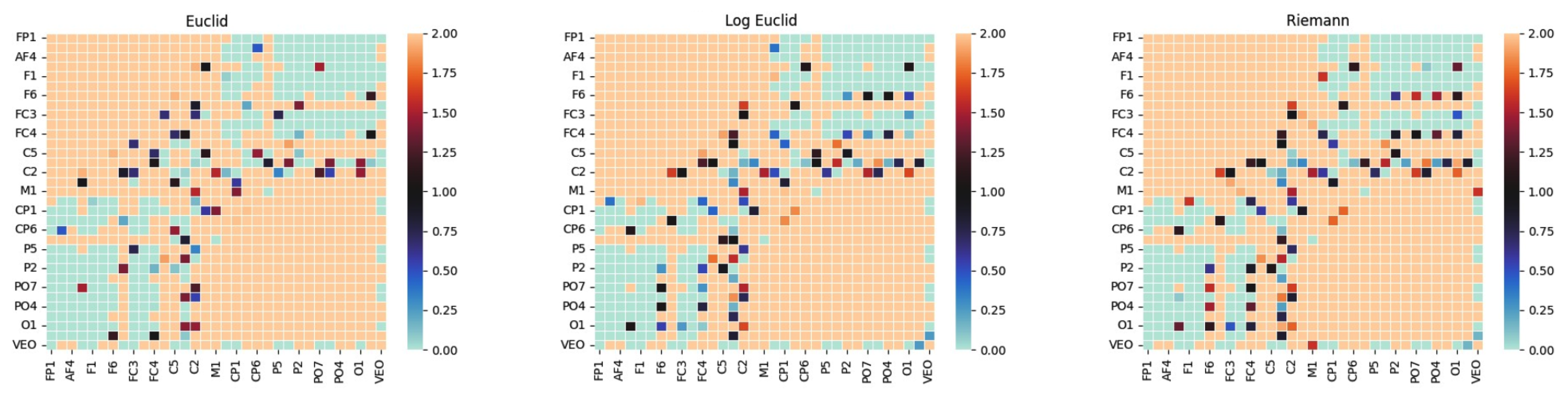
Figure A2.
Confusion matrices for fgMDM classifier across (a) Session 1, (b) Session 2 and (c) Session 3. Cell values are percentages.
Figure A2.
Confusion matrices for fgMDM classifier across (a) Session 1, (b) Session 2 and (c) Session 3. Cell values are percentages.
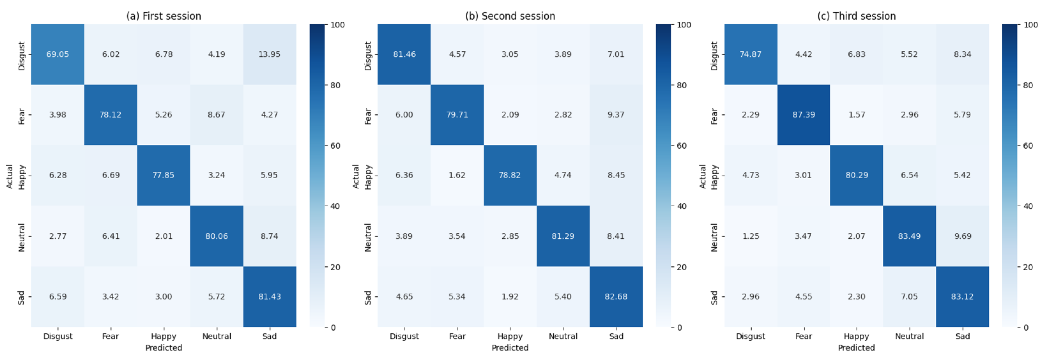
Figure A3.
Confusion matrices for the SVM classifier across (a) Session 1, (b) Session 2 and (c) Session 3. Cell values are percentages.
Figure A3.
Confusion matrices for the SVM classifier across (a) Session 1, (b) Session 2 and (c) Session 3. Cell values are percentages.
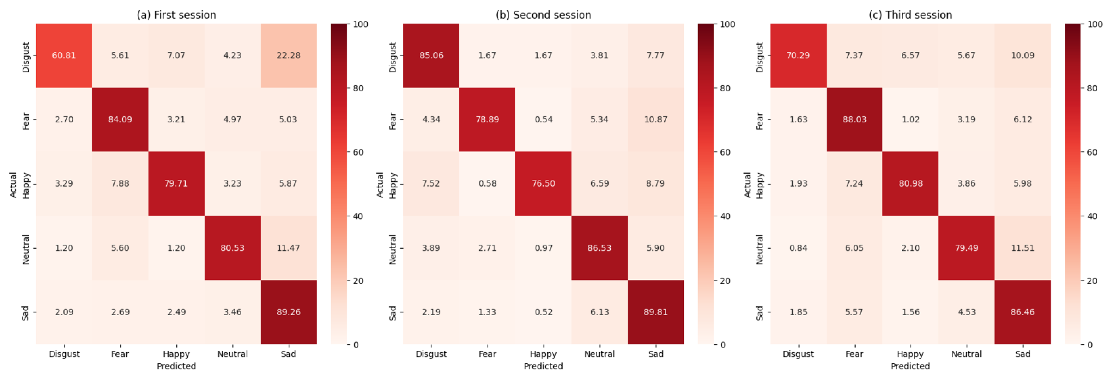
Figure A4.
Per-participant average accuracy for FgMDM (orange) and SVM (blue).
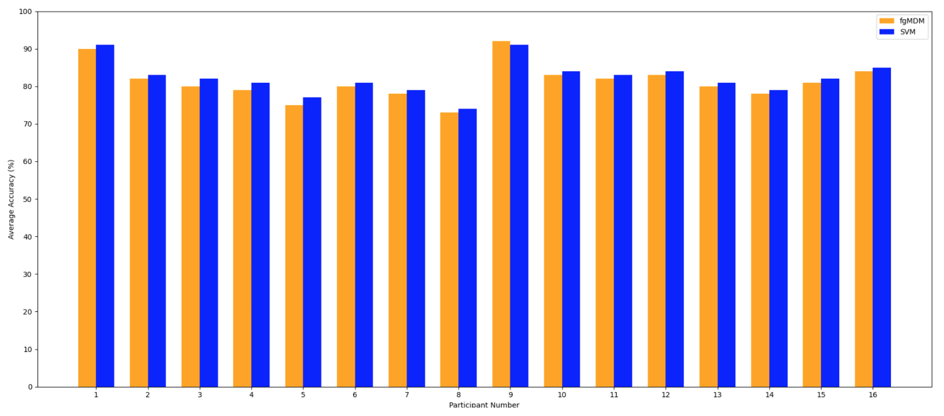
Figure A5.
Correlation between classification accuracies and self-assessment scores
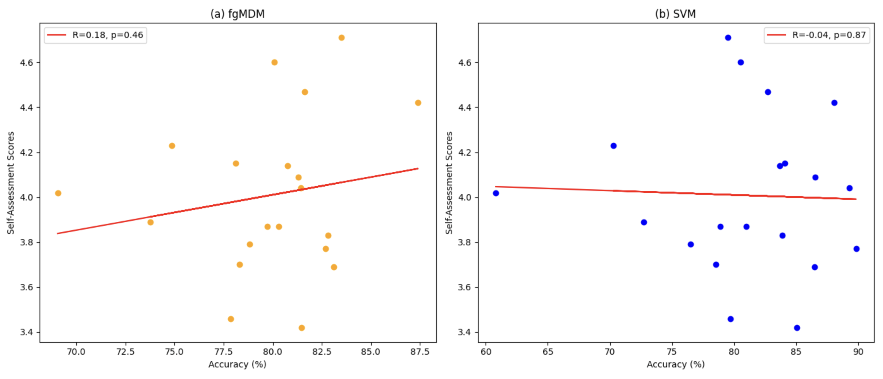
Figure A6.
Confusion matrices reported by previous studies on the SEED-V dataset. Darker cells indicate higher classification accuracy.
Figure A6.
Confusion matrices reported by previous studies on the SEED-V dataset. Darker cells indicate higher classification accuracy.
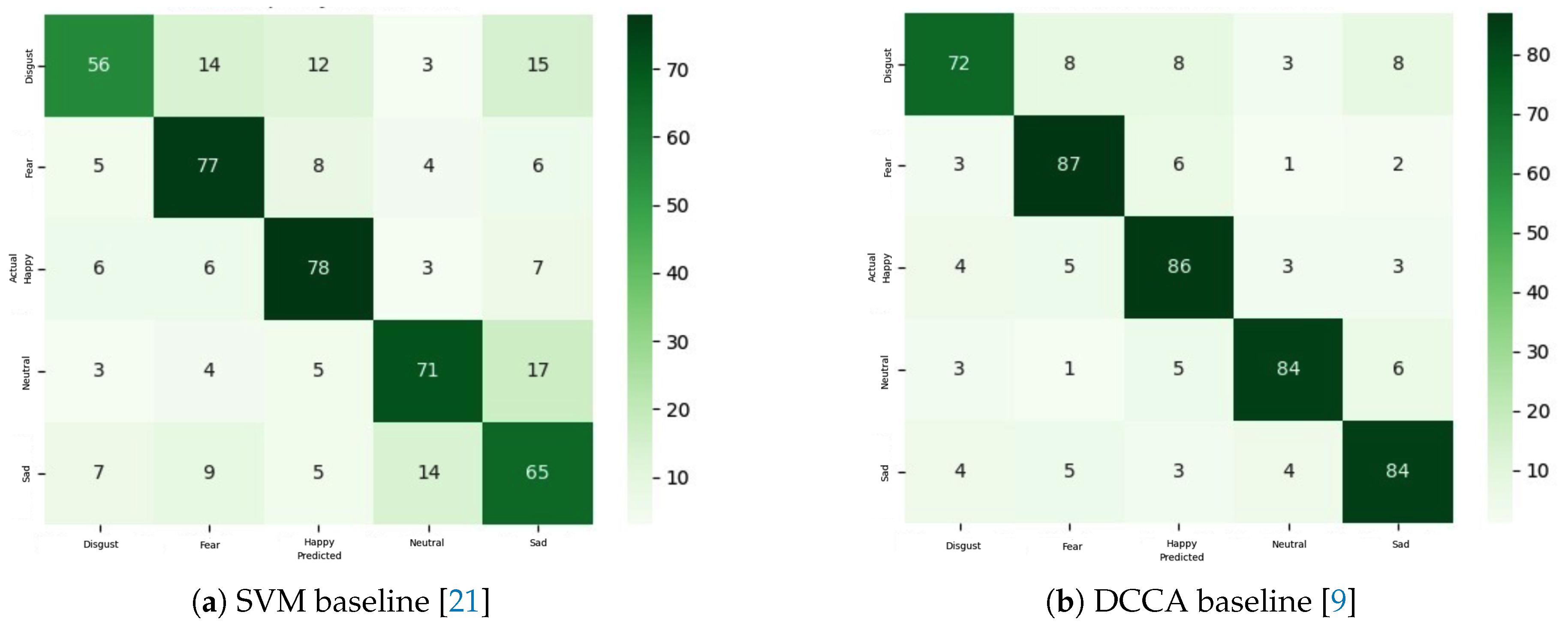

Table A1.
Average Ratings for Each Emotion Category by Participant
| Participant | Happiness | Sadness | Fear | Neutral | Disgust |
|---|---|---|---|---|---|
| 1 | 3.2 | 3.4 | 3.9 | 4.7 | 3.1 |
| 2 | 4.0 | 4.3 | 4.1 | 4.7 | 3.3 |
| 3 | 4.4 | 4.7 | 4.2 | 4.7 | 4.2 |
| 4 | 3.2 | 3.7 | 4.8 | 4.8 | 3.2 |
| 5 | 3.3 | 3.8 | 3.9 | 5.0 | 4.6 |
| 6 | 3.3 | 4.1 | 3.8 | 4.8 | 3.8 |
| 7 | 3.3 | 3.6 | 4.0 | 4.1 | 3.4 |
| 8 | 4.2 | 4.6 | 4.8 | 5.0 | 4.2 |
| 9 | 4.1 | 5.0 | 4.8 | 4.4 | 4.3 |
| 10 | 4.0 | 3.0 | 4.3 | 3.7 | 4.3 |
| 11 | 4.6 | 3.9 | 4.0 | 4.7 | 4.6 |
| 12 | 4.3 | 3.7 | 4.0 | 5.0 | 4.4 |
| 13 | 1.9 | 3.4 | 3.8 | 4.9 | 3.5 |
| 14 | 4.1 | 3.7 | 4.6 | 4.7 | 4.6 |
| 15 | 3.9 | 3.4 | 4.1 | 4.6 | 3.0 |
| 16 | 3.3 | 3.0 | 4.2 | 4.6 | 3.6 |
Table A2.
Number of Samples for Each Emotion by Session
| Session | Happiness | Sadness | Disgust | Fear | Neutral |
|---|---|---|---|---|---|
| 1 | 93 | 131 | 82 | 106 | 100 |
| 2 | 54 | 69 | 82 | 108 | 90 |
| 3 | 74 | 123 | 63 | 123 | 85 |
| Total | 221 | 323 | 227 | 337 | 275 |
Table A3.
Performance Metrics for the fgMDM Classifier
| Session | Accuracy | Precision | Recall | F1 Score |
|---|---|---|---|---|
| 1 | 0.778 | 0.777 | 0.773 | 0.775 |
| 2 | 0.811 | 0.814 | 0.808 | 0.811 |
| 3 | 0.826 | 0.826 | 0.818 | 0.822 |
Table A4.
Performance Metrics for SVM in Tangent Space
| Session | Accuracy | Precision | Recall | F1 Score |
|---|---|---|---|---|
| 1 | 0.753 | 0.767 | 0.741 | 0.754 |
| 2 | 0.845 | 0.860 | 0.833 | 0.847 |
| 3 | 0.783 | 0.794 | 0.768 | 0.781 |
Table A5.
Computational Time for FgMDM and SVM Classifiers
| Session | FgMDM (seconds) | SVM (seconds) |
|---|---|---|
| 1 | 58.294 | 39.393 |
| 2 | 44.972 | 32.841 |
| 3 | 72.184 | 62.381 |
Table A6.
Classification Accuracy for All Patients with Average Ratings Given to Films During Individual Sessions
Table A6.
Classification Accuracy for All Patients with Average Ratings Given to Films During Individual Sessions
| Session 1 | Session 2 | Session 3 | Aggregate | |||||||||
|---|---|---|---|---|---|---|---|---|---|---|---|---|
| Emotion | Score | FgMDM | SVM | Score | FgMDM | SVM | Score | FgMDM | SVM | Score | FgMDM | SVM |
| Disgust | 4.02 | 69.05 | 60.81 | 3.42 | 81.46 | 85.06 | 4.23 | 74.87 | 70.29 | 3.89 | 74.29 | 72.54 |
| Fear | 4.15 | 78.12 | 84.09 | 3.87 | 79.71 | 78.89 | 4.42 | 87.39 | 88.03 | 4.14 | 81.39 | 84.11 |
| Happy | 3.46 | 77.85 | 79.71 | 3.79 | 78.82 | 76.50 | 3.87 | 80.29 | 80.98 | 3.71 | 78.66 | 79.27 |
| Neutral | 4.60 | 80.06 | 80.53 | 4.58 | 81.29 | 86.53 | 4.71 | 83.49 | 79.49 | 4.63 | 81.23 | 82.32 |
| Sad | 4.04 | 81.43 | 89.26 | 3.77 | 82.68 | 89.81 | 3.69 | 83.12 | 86.46 | 3.83 | 82.11 | 88.54 |
Disclaimer/Publisher’s Note: The statements, opinions and data contained in all publications are solely those of the individual author(s) and contributor(s) and not of MDPI and/or the editor(s). MDPI and/or the editor(s) disclaim responsibility for any injury to people or property resulting from any ideas, methods, instructions or products referred to in the content. |
© 2025 by the authors. Licensee MDPI, Basel, Switzerland. This article is an open access article distributed under the terms and conditions of the Creative Commons Attribution (CC BY) license (http://creativecommons.org/licenses/by/4.0/).
Copyright: This open access article is published under a Creative Commons CC BY 4.0 license, which permit the free download, distribution, and reuse, provided that the author and preprint are cited in any reuse.


