1. Introduction
With the rapid advancement of modern science and technology, human emotion has become a key indicator of an individual’s mental state and emotional response to events, shaped by subjective experience [
1]. Emotion-related expression plays a crucial role in human communication and holds significant potential across various industries, including healthcare, gaming, and psychology. As a result, researchers are increasingly focused on developing methods to enhance computers’ ability to interpret human emotions during interactions with operators [
2]. To achieve this, creating robust emotion recognition algorithms is essential for enabling machines to accurately detect and understand emotional states, facilitating more intuitive human-computer interactions. While emotions are typically conveyed through facial expressions or auditory cues—common methods by which humans recognize emotions in others [
3]—recent research has shifted toward utilizing physiological signals for more direct detection of emotional states [
4]. These signals, such as heart rate (ECG/EKG), respiratory rate and content (capnogram), skin conductance (EDA), muscle activity (EMG), and brain electrical activity (EEG), are produced by the body’s physiological processes. Among these, electroencephalography (EEG) stands out as one of the most widely used physiological signals for analyzing emotional states [
5].
Electroencephalography (EEG) refers to the recording of the brain’s spontaneous electrical activity over time, captured from multiple electrodes placed on the scalp. In the healthcare industry, EEG is used to detect abnormal brain activity and diagnose conditions such as epilepsy, brain tumors, strokes, and sleep disorders. The recordings are obtained by placing electrodes on the scalp, with electrode locations and names typically specified by the International 10-20 [
6] system for most clinical and research applications. The ”10” and ”20” refer to the distances between adjacent electrodes, which are either 10% or 20% of the total front-back or right-left distance of the skull. This system helps ensure consistency and accuracy in brainwave recording, and is used in datasets such as DEAP dataset for emotion analysis.
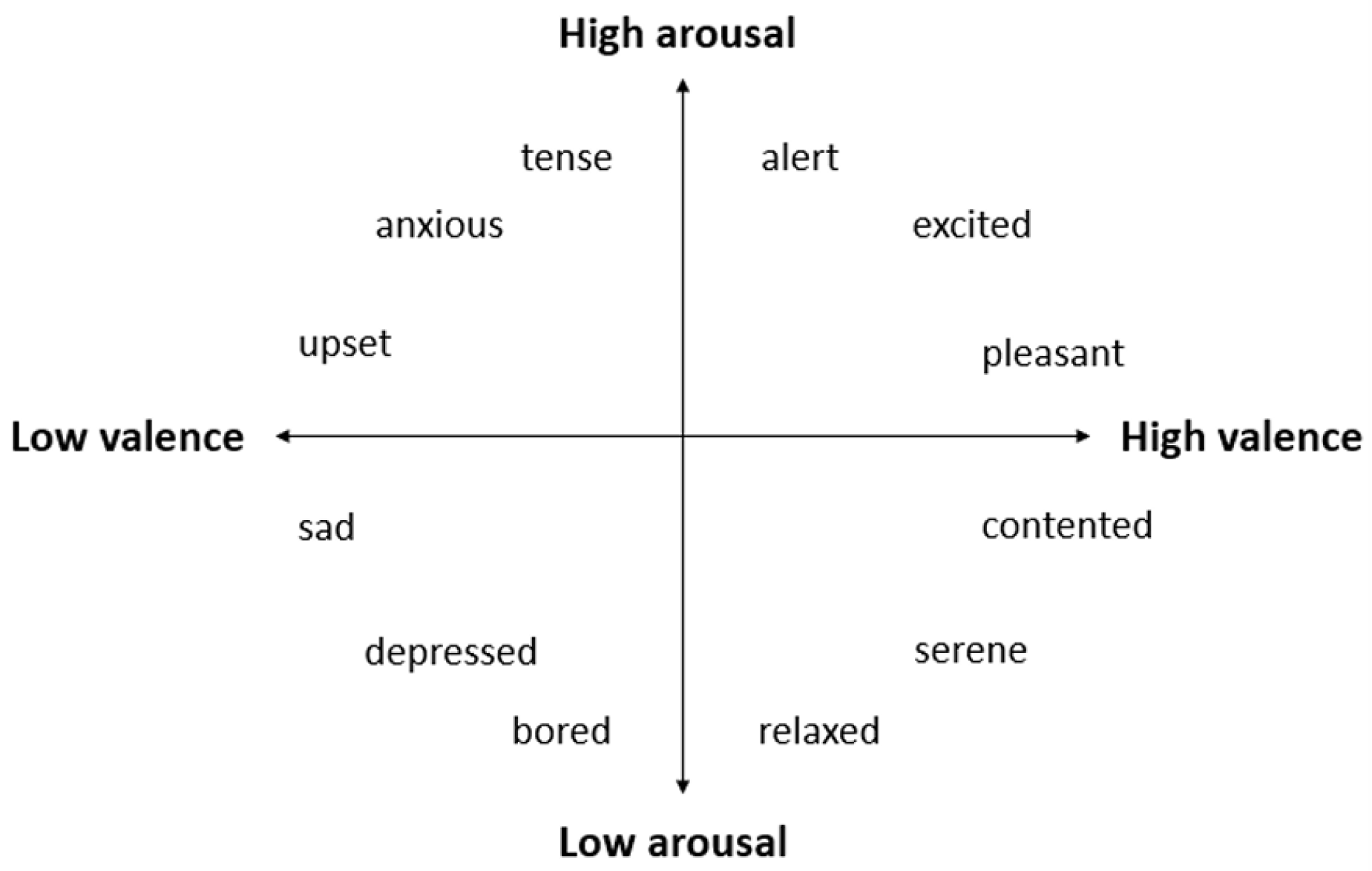
This study focuses on EEG-based emotion recognition, specifically examining the valence and arousal dimensions to classify emotional states. Valence refers to the positivity or negativity of an emotional response, while arousal measures the intensity or activation level of the emotion. These two dimensions are essential for understanding the spectrum of human emotions, as they encompass both the quality and intensity of emotional experiences [
7]. Using the DEAP dataset, which includes EEG data collected from participants exposed to emotional stimuli like music videos [
8], the research aims to enhance emotion recognition algorithms and deepen the understanding of how emotional states can be detected and classified from brain activity. The findings could have applications in healthcare, human-computer interaction, and psychological research.
2. Related Works
EEG has been well-studied to investigate how the brain reacts to emotional experiences [
9], offering valuable insights into the neural mechanisms underlying emotions. As a non-invasive method, EEG captures electrical activity in the brain, providing high temporal resolution data that makes it suitable for studying dynamic emotional states. Leveraging this potential, numerous researchers have developed machine learning and deep learning techniques to decode emotional responses from EEG signals.
Among the many studies utilizing the DEAP dataset, the work by Chen et al. [
10] explored the potential of Convolutional Neural Networks (CNNs) for emotion recognition. This study employed a subject-dependent approach focusing on the valence and arousal dimensions. By training CNNs on features extracted from EEG signals, the model achieved impressive accuracies of 85.57% for arousal and 88.76% for valence.
Similarly, Alhagry et al. [
11] adopted Long Short-Term Memory (LSTM) networks to process the sequential nature of EEG signals. Using a subject-dependent approach with four-fold cross-validation, this study targeted the valence, arousal, and liking dimensions, achieving accuracies of 85.65%, 85.45%, and 87.99%, respectively. The results demonstrate the importance of capturing temporal dependencies in EEG signals for more accurate emotion classification.
To integrate complementary techniques, Li et al. [
12] proposed a hybrid approach combining these models to analyze EEG signals. By leveraging CNNs for spatial feature extraction and LSTMs for temporal modeling, the study achieved an accuracy of 75.21% in classifying four emotional states (high valence-high arousal, high valence-low arousal, low valence-high arousal, and low valence-low arousal).
Moreover, Xing et al. [
13] introduced a framework that combined Stacked Autoencoders (SAE) with LSTM networks to focus on subject-independent emotion recognition. Using 10-fold cross-validation, this study achieved accuracies of 81.10% for valence and 74.38% for arousal. The use of SAE for unsupervised feature learning followed by LSTM for temporal pattern analysis allowed for robust emotion recognition across multiple subjects.
In addition, this study [
14] introduced a model combining AlexNet and DenseNet for feature extraction, PCA for dimensionality reduction, and SVM for classification. Evaluated on the DEAP and EEG Brainwave datasets, it achieved accuracies of 95.54% (valence) and 97.26% (arousal) for DEAP, and 98.42% overall for EEG Brainwave, outperforming existing methods in key metrics.
Lastly, this study [
15]leverages sample- and epoch-level attention mechanisms to enhance EEG-based emotion classification. The model achieved 69.3% accuracy on 0.5-s EEG segments, surpassing baseline LSTM models by 4.8% and demonstrating robustness against EEG non-stationarity with longer epochs.
Collectively, These studies highlight the DEAP dataset’s versatility and the evolution of EEG-based emotion recognition, showcasing diverse approaches—from CNNs and LSTMs to hybrid models—advancing the accuracy and understanding of emotional states through brain activity.
3. Methods And Materials
3.1. Dataset Overview
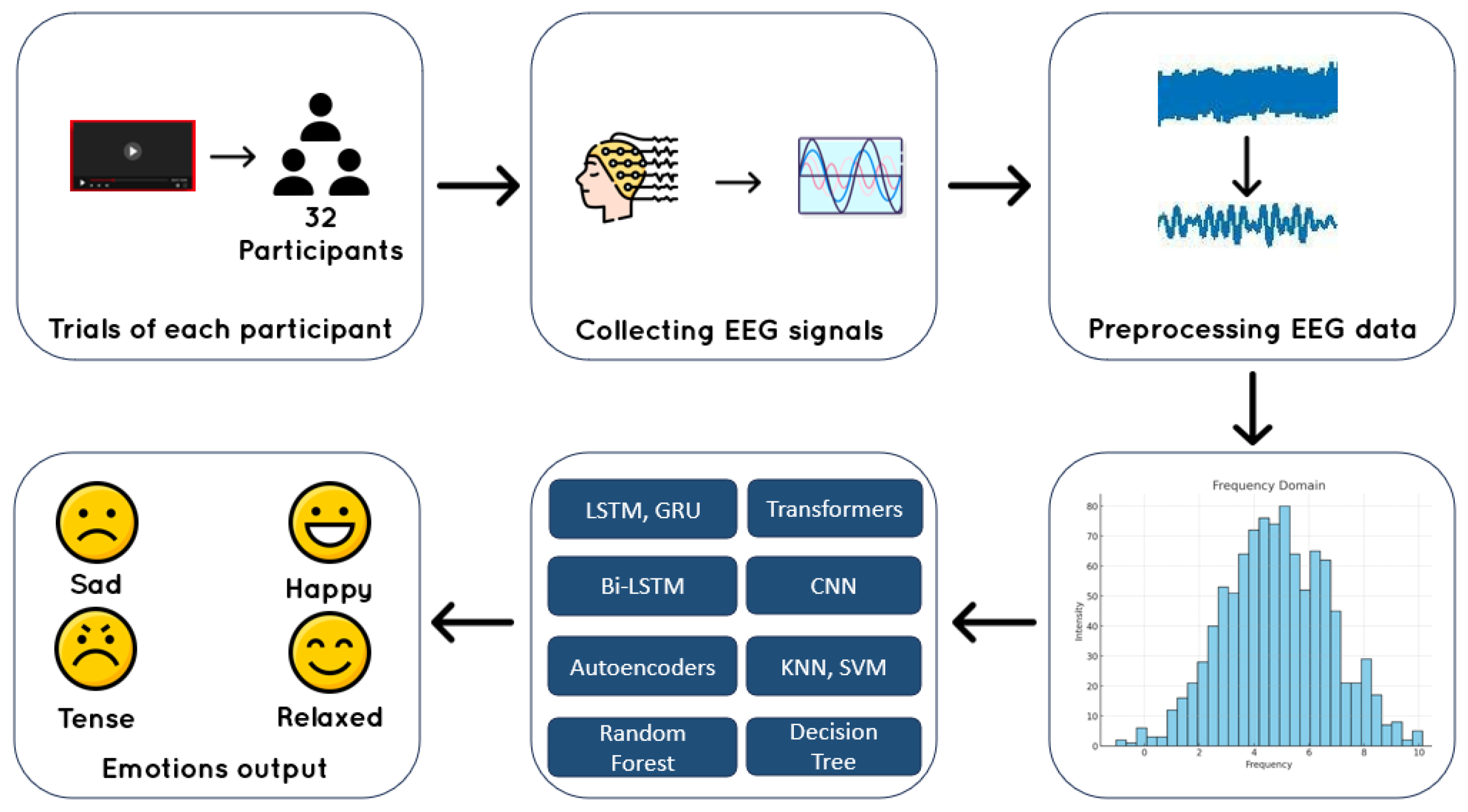
The DEAP (Database for Emotion Analysis using Physiological Signals) dataset [
8] comprises data from 32 participants, each undergoing 40 trials where they were exposed to emotional stimuli through 60-second music videos. The same set of videos was presented to all participants, but the order was randomized to minimize order effects while ensuring consistent stimuli across trials.
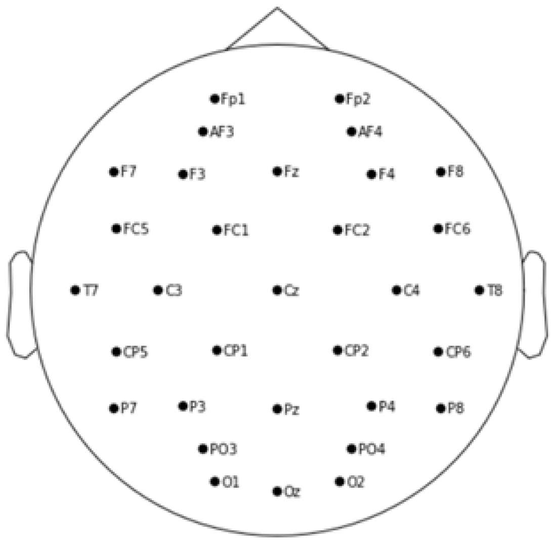
EEG data was recorded at a sampling rate of 128 Hz across 32 channels: Fp1, AF3, F3, F7, FC5, FC1, C3, T7, CP5, CP1, P3, P7, PO3, O1, OZ, PZ, Fp2, AF4, FZ, F4, F8, FC6, FC2, CZ, C4, T8, CP6, CP2, P4, P8, PO4, and O2. Each trial measured four emotional dimensions — valence, arousal, liking, and dominance — immediately after watching a music video [
16].
Figure 1.
The Electrodes placement on the scalp.
Figure 1.
The Electrodes placement on the scalp.
For emotion classification, valence and arousal were categorized into "high" or "low" groups based on predefined thresholds, which facilitated the analysis of emotional responses. This classification scheme enabled the collection of EEG data across a standardized set of emotional stimuli, ensuring that participants’ responses to the same content were evaluated consistently [
17]. Furthermore, it allowed for the consideration of potential variability introduced by the order in which the stimuli were presented. In the current study, we adopted specific thresholds to define the emotional states: a valence value greater than 6.5 was categorized as high valence, while values less than or equal to 6.5 were classified as low valence. Similarly, arousal values exceeding 6.5 were considered high arousal, while values less than or equal to 6.5 were classified as low arousal. This approach ensures a standardized method of categorization that aligns with established practices in emotion recognition research.
Figure 2.
2-Dimension emotions’ model.
Figure 2.
2-Dimension emotions’ model.
3.2. Signal Preprocessing And Feature Extraction
For EEG signal preprocessing, various approaches are employed to minimize noise and artifacts, enabling accurate analysis of emotional states.
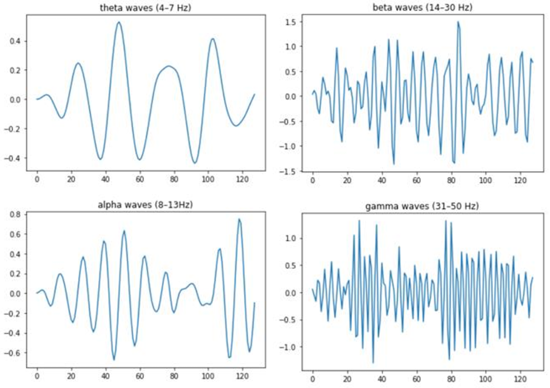
Bandpass filtering is a fundamental preprocessing technique in EEG analysis for emotion recognition, as it isolates specific neural frequency bands associated with distinct mental and emotional states. These bands include Delta (0.5–4 Hz), linked to deep sleep and healing; Theta (4–8 Hz) and Alpha (8–13 Hz), critical for detecting emotions like relaxation, creativity, and calmness; and Beta (13–30 Hz) and Gamma (30–100 Hz), associated with heightened arousal, learning, and emotional integration [
18]. By filtering the signals to focus on these relevant frequencies, bandpass filtering reduces noise and eliminates irrelevant artifacts, thereby enhancing the quality of EEG data for analysis. This technique has been widely adopted in emotion recognition research to improve system sensitivity to emotional states such as stress or relaxation, enabling more accurate classification. demonstrate that concentrating on these frequency bands significantly improves the detStudies [
20,
21]ection of emotional responses.
Figure 3.
Visualization of EEG frequency bands.
Figure 3.
Visualization of EEG frequency bands.
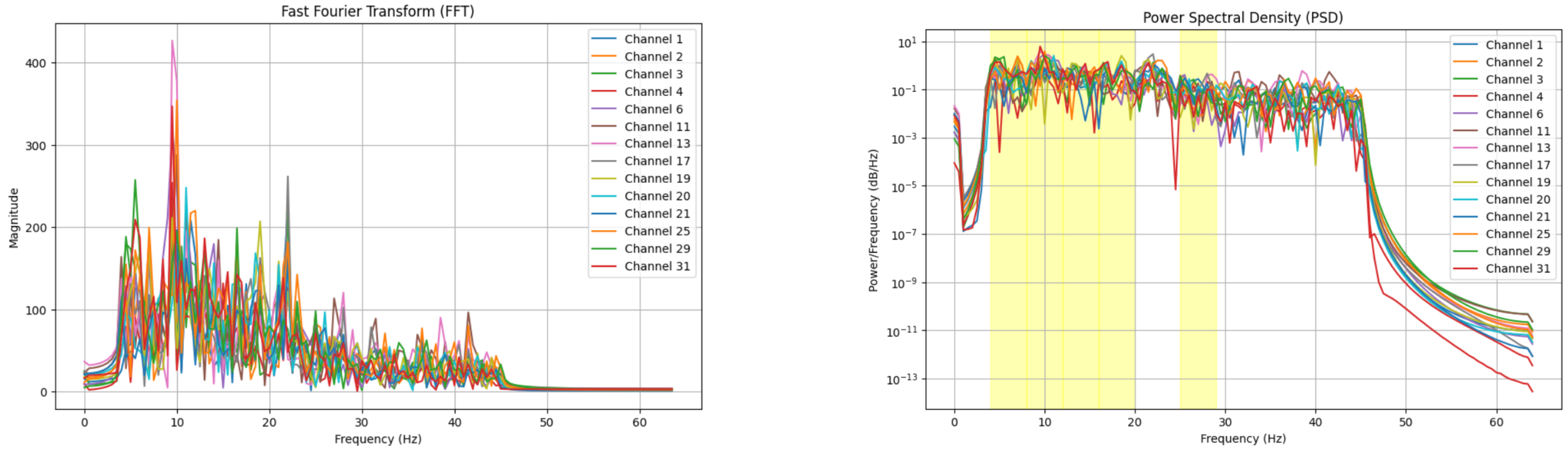
After bandpass filtering, Power Spectral Density (PSD) estimation is performed to analyze the power distribution within each frequency band, providing valuable features for emotion classification. Welch’s method, a widely used approach for PSD calculation, reduces noise by averaging the periodograms of overlapping signal segments, resulting in a smoother and more reliable estimate. This method highlights the energy contained in each frequency band—such as Alpha, Beta, and Gamma—offering insights into how different neural frequencies contribute to emotional states. The PSD is calculated using the formula:
Where
represents the time-domain EEG signal,
F denotes the Fourier transform, and * indicates the convolution operation [
19]. By quantifying the power within each frequency band, PSD estimation allows researchers to link brain activity to emotional processing. Extracting these power values enables the classification of emotional states and enhances our understanding of how the brain responds to various emotional stimuli [
22].
Figure 4.
Frequency domain analysis of EEG signals.
Figure 4.
Frequency domain analysis of EEG signals.
Finally, standardization is a key step to ensure that the features are consistent and comparable across different subjects and sessions. Since EEG signals can vary in amplitude and individual brain activity patterns can differ from person to person, standardization helps to mitigate these discrepancies and ensure that no one feature dominates the learning process. In this context, standardization involves scaling the power values of the different frequency bands—Delta, Theta, Alpha, Beta, and Gamma—so that each feature has a mean of zero and a standard deviation of one [
23]. This step is particularly important for machine learning models, as it prevents any one feature from disproportionately influencing the model’s learning process due to differences in signal magnitudes across subjects or channels. After standardizing the data, the features are reshaped to meet the input requirements of deep learning models, ensuring they are properly formatted for emotion classification tasks. This final step in the preprocessing pipeline ensures that the model can effectively learn from the relevant patterns associated with emotional responses, leading to more accurate predictions [
24].
By carefully applying these preprocessing steps—bandpass filtering to isolate key frequency bands, PSD estimation to quantify the power in those bands, and standardization to ensure consistency—we are able to extract high-quality features from EEG signals that provide valuable insights into emotional processing. These techniques form the foundation of our emotion recognition pipeline, allowing us to build robust models that can accurately classify emotional states based on brain activity patterns [
25].
Figure 5.
The pipeline used in this study.
Figure 5.
The pipeline used in this study.
3.3. Implementation Tools And Libraries
Implementing emotion recognition models with EEG data relies on robust tools for efficient processing, feature extraction, model development, and evaluation. Key Python libraries used in this study include MNE for EEG preprocessing, Pickle for data storage, Keras for deep learning, SciPy for scientific computing, and Scikit-learn for machine learning tasks. While each of these libraries is well-regarded for its specific capabilities, this study focuses particularly on MNE due to its specialization in EEG signal processing. MNE offers a comprehensive set of tools for processing, analyzing, and visualizing EEG data, making it invaluable for tasks like filtering, epoching, and feature extraction. Its robust functionality for bandpass filtering enables the isolation of frequency bands—Delta, Theta, Alpha, Beta, and Gamma—which are crucial for understanding emotional processing. This specialization makes MNE a standout choice for emotion recognition research [
26].
4. Methodology
4.1. First Implementation
Initial experiments employed classical machine learning algorithms, including K-Nearest Neighbors (KNN), Support Vector Machines (SVM), Decision Trees (DT), and Random Forests (RF), to classify emotional states based on EEG data. The EEG data was reshaped into a 3D array format (1280, 32, 8064) where 1280 designs trials 40*32, the channels are 32 channel, and time samples for efficient processing. Corresponding labels were transformed into a 2D array to align with the binary classification task.
While these models achieved high training accuracy, they struggled with generalization to unseen data, indicating overfitting. This limitation highlights the challenge of effectively capturing the complex and non-linear patterns in EEG signals, necessitating the adoption of more advanced techniques, such as deep learning, to improve performance and robustness.
4.2. Second Implementation
For our second implementation, We have used some advanced deep learning techniques. The methodology is organized into several key stages, including data preprocessing, feature extraction, model development, and training.
The dataset was prepared by shuffling the EEG signals and their corresponding labels to ensure randomness and prevent any bias during model training. The data was transformed into vector form using a custom function to enable efficient processing by the models. The transformed vectors were subsequently used for dimensionality reduction and feature extraction.
To reduce the dimensionality of the input data while preserving its critical features, an autoencoder was constructed with the following architecture:
Input Layer: Accepts vectors of size 32.
Encoding Layers: A dense layer of size 64 followed by a bottleneck layer to compress the data further.
Decoding Layers: Two dense layers to reconstruct the data back to its original dimension.
The autoencoder was trained using the Mean Squared Error (MSE) loss and the Stochastic Gradient Descent (SGD) optimizer. The Mean Squared Error (MSE) loss function is defined as:
The Stochastic Gradient Descent (SGD) optimization process is expressed as:
The encoder component of the autoencoder was isolated and used to encode the input data into a lower-dimensional feature space for subsequent analysis.
The encoded EEG data was subjected to feature extraction by calculating band power features from the encoded signals. This process generated a robust feature set, which was organized into a new dataset for model training. The feature dataset was then split into training and testing sets in a 90:10 ratio using stratified sampling to maintain label distribution.
A Transformer model was developed for the classification task. The architecture included:
Input Layer: Accepts the input of shape.
Transformer Encoder: Implements multi-head attention with 4 heads and a feed-forward network with 128 dimensions. Dropout regularization and layer normalization were applied for improved generalization and stability.
Global Pooling: Reduces the sequence dimension to create a fixed-size feature vector.
Dense Layers: Includes a 64-unit dense layer with ReLU activation followed by a single-unit output layer with a sigmoid activation for binary classification.
The model was compiled using the Adam optimizer with binary cross-entropy loss and trained over 30 epochs with a batch size of 16.
To leverage temporal dependencies and contextual information, a hybrid model combining LSTM and Transformer layers was developed:
LSTM Layer: Captures temporal patterns in the input data.
Transformer Encoder: Adds contextual attention mechanisms on top of the LSTM outputs.
Global Pooling and Dense Layers: Similar to the Transformer model.
A variation of the hybrid model incorporated positional encoding to enhance temporal feature representation. Positional encoding was implemented as a sine-cosine function, applied to the input data prior to processing by the LSTM and Transformer layers. An additional hybrid model variant combined LSTM and Transformer outputs using an additive layer before the final dense layers.
All models were trained on GPUs to expedite computation. The Adam optimizer was used with a learning rate scheduler for improved convergence. Training involved 30-40 epochs with batch sizes ranging from 16 to 32. Performance was evaluated using accuracy metrics, with validation accuracy monitored to determine the highest-performing model.
4.3. Third Implementation
For the third implementation of some deep learning architectures, we have implemented severals ones to see what’s the best deep learning architecture that will give us the best results, however each one of these archirectures is different from the other one, we have implemented a GRU model, CNN model, BiLSTM model.
For each implemetation of these, we used only the data from six participants (subject IDs: 01 to 06) are analyzed instead of the whole 32 participants. The EEG signals are recorded at a sampling rate of 128 Hz, with 32 electrodes measuring brain activity, where we selected only 14 EEG channels based on their relevance to emotion recognition. Six frequency bands (‘theta’, ‘alpha’, ‘beta’, ‘delta’, ‘gamma’) were chosen, as they correlate with cognitive and emotional states.
To extract meaningful features, a sliding window of 2 seconds (256 samples) with a step size of 0.125 seconds (16 samples) was applied to the EEG data. For each window and selected channel, the FFT was computed to estimate the band power across the six frequency bands. These band power features were then concatenated into a single vector representing the window’s characteristics. Each feature vector was paired with the corresponding trial labels provided in the dataset, forming the basis for further processing and model training.
To train and test the models, The data was split into training (75%) and testing (25%) sets by sampling 1 in 4 trials for testing and using the remaining for training. This ensured no overlap between training and testing samples.
Features were normalized to ensure consistency across samples. Both training and testing datasets were standardized to remove bias from the different ranges of feature values.
Labels for arousal and valence dimensions were thresholded at 6.5 (on a scale of 1 to 9) to create binary classification targets: High arousal/valence equals to ’1’ while Low arousal/valence equals to ’0’.
The Bidirectional LSTM model is designed to capture temporal dependencies in EEG signals by processing sequences from both directions, allowing it to learn past and future contexts simultaneously. The input layer accepts sequences of EEG data with a specified number of features. The BiLSTM layers consist of an initial 128-unit layer, followed by a stack of LSTM layers with 256, 64, 64, and 32 units. These layers enable the model to capture both short- and long-term dependencies in the data. Dropout layers are applied after each LSTM layer to prevent overfitting and improve the model’s generalization ability. The model concludes with fully connected dense layers: a 16-unit layer followed by a sigmoid activation function for binary classification, outputting whether the input signal corresponds to one emotion or another.
The 1D CNN model is tailored to extract spatial patterns from EEG data by applying convolutional filters that learn local feature representations. The input layer processes sequences of EEG signals with a specified number of features. The model contains three convolutional layers, each applying 128, 128, and 64 filters respectively, with a kernel size of 3 and ReLU activation to introduce non-linearity. To improve the model’s convergence and prevent overfitting, batch normalization is applied after each convolutional layer. MaxPooling layers are used to downsample the feature maps by a factor of 2, reducing the computational complexity and retaining important features. The final layers consist of dense layers with 64, 32, and 16 units, each followed by dropout layers to regularize the model. A sigmoid activation function at the output layer provides the binary classification result.
The GRU model leverages the Gated Recurrent Unit (GRU) architecture, which is designed to effectively handle long sequences of data by preserving important temporal information while reducing the computational complexity compared to LSTMs. The input layer processes sequences of EEG signals, each with a specified number of features. The GRU architecture consists of an initial layer with 128 units, followed by additional GRU layers with 256, 64, 64, and 32 units. These layers process the data sequentially, capturing temporal dependencies in the input. Dropout layers are applied after each GRU layer to improve the model’s ability to generalize and to mitigate overfitting. The model concludes with a fully connected dense layer containing 16 units, followed by a sigmoid activation function for binary classification. This architecture is specifically tailored to analyze EEG sequences and classify them by learning both temporal and spatial patterns within the data.
All models were compiled using the binary cross-entropy loss function due to the binary nature of the output labels. The Adam optimizer was used for efficient gradient-based optimization
The models were trained on the normalized and standardized data, with early stopping and dropout layers employed to mitigate overfitting. Each model’s performance was compared to identify the best architecture for emotion recognition using EEG data.
4.4. eXplainable Artificial Intelligence (XAI)
In our research, we applied SHapley Additive exPlanations (SHAP) to make our deep learning model, a Bidirectional LSTM trained on the DEAP dataset, more interpretable. SHAP, a method derived from Shapley values in game theory, offers a systematic way to explain the predictions of machine learning models. In this analogy, the model is considered the “game,” and the “players” are the input features—specifically, the EEG signal characteristics extracted from the DEAP dataset.
SHAP assigns a significance score to each feature, representing its impact on the model’s predictions. This approach helped us pinpoint which EEG features were most critical in predicting emotional states, such as arousal, valence, and dominance, which are central measures in the DEAP dataset. By providing explanations at the individual sample level, SHAP highlights the contribution of each feature to a specific prediction. These insights can then be combined to form a comprehensive view of how the model operates, enhancing the transparency of its decision-making process.
Through this technique, we identified the EEG features that the Bidirectional LSTM prioritized for emotion classification. Using SHAP, we visualized the role these features played in shaping the model’s outputs, a vital step toward fostering confidence in automated emotion recognition systems [
27].
5. Results & Discussion
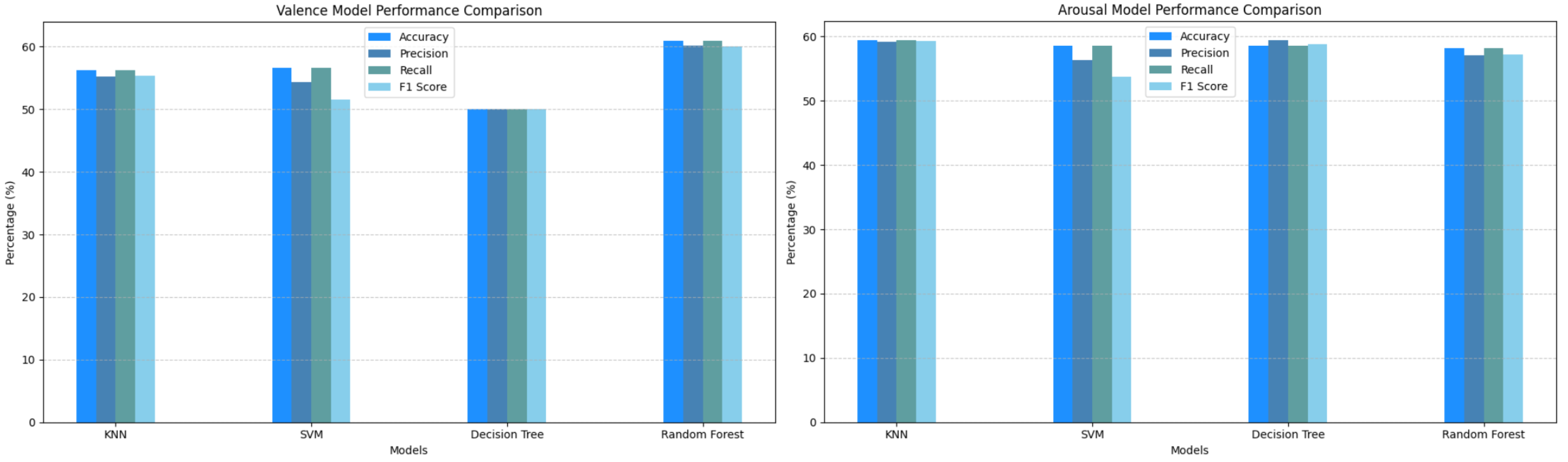
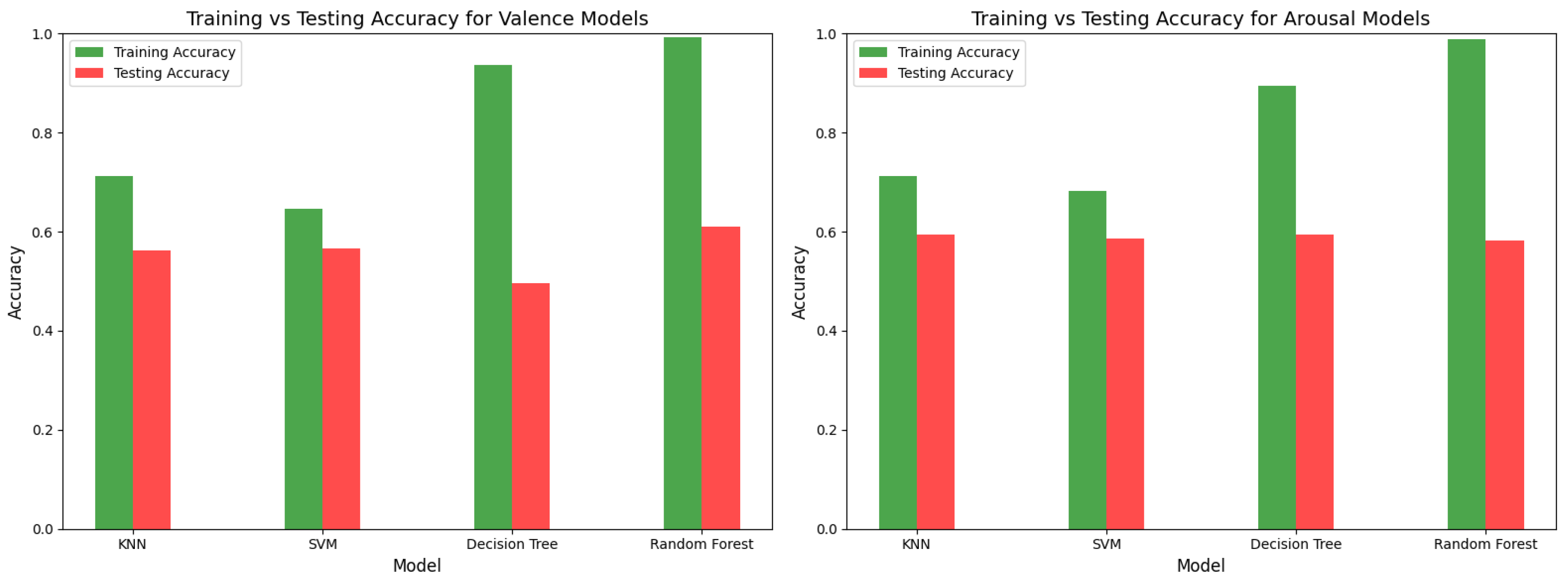
In the initial implementation, which involved classical machine learning models, we observed high training accuracy, particularly for Decision Trees and Random Forest. In contrast, K-Nearest Neighbors (KNN) and Support Vector Machines (SVM) demonstrated moderate training accuracy. However, testing accuracy across all models was notably low, not exceeding 60%, indicating that the models suffered from overfitting.
Figure 6 and
Figure 7 provide detailed visualizations of the models’ performance, while
Table 1 summarizes their respective accuracy metrics for both valence and arousal.
The implementation of machine learning models served as an initial step to evaluate whether more advanced preprocessing and deep learning techniques were required. During this exploration, we identified autoencoders as a promising tool [
28]. By using an autoencoder, we reduced the high-dimensional EEG data into a lower-dimensional representation, making it more manageable for processing. Despite this reduction, the autoencoder effectively retained the diagnostically significant features essential for disease classification. This dimensionality reduction not only simplified the training process for the LSTM model but also enhanced its performance by emphasizing the most informative features of the data.
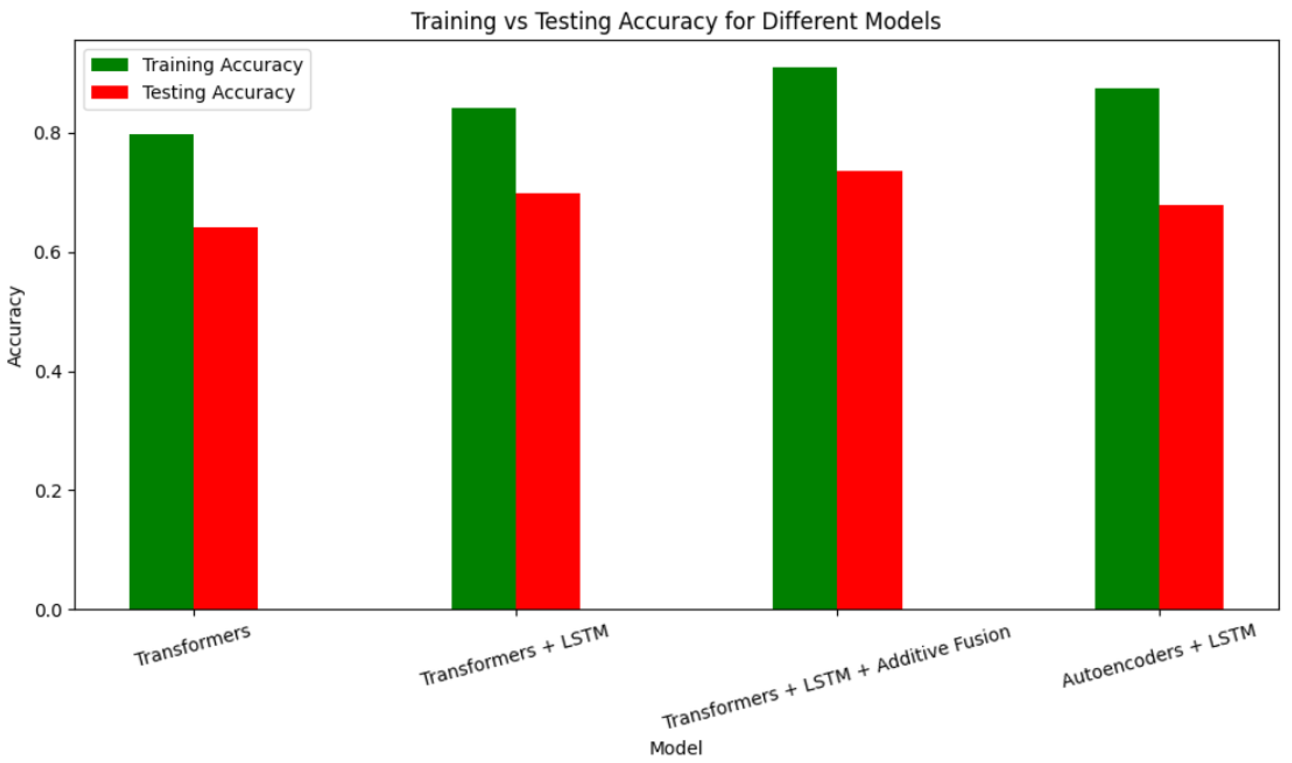
As shown in
Figure 8, the autoencoder-enabled model achieved a commendable training accuracy; however, the testing accuracy was moderate, indicating room for improvement. To address this, we explored a different approach: integrating transformers with other architectures such as LSTM and additive fusion. Our findings revealed that combining architectures led to progressively higher accuracy, as demonstrated in the results presented in the table below.
Table 2.
Accuracy comparison of different hybrid models.
Table 2.
Accuracy comparison of different hybrid models.
| Models |
Training Accuracy |
Testing Accuracy |
| Transformers |
79.85% |
64.15% |
| Transformers + LSTM |
84.26% |
69.81% |
| Transformers + LSTM + additive fusion |
90.98% |
73.58% |
| LSTM + Autoencoders |
87.56% |
67.88% |
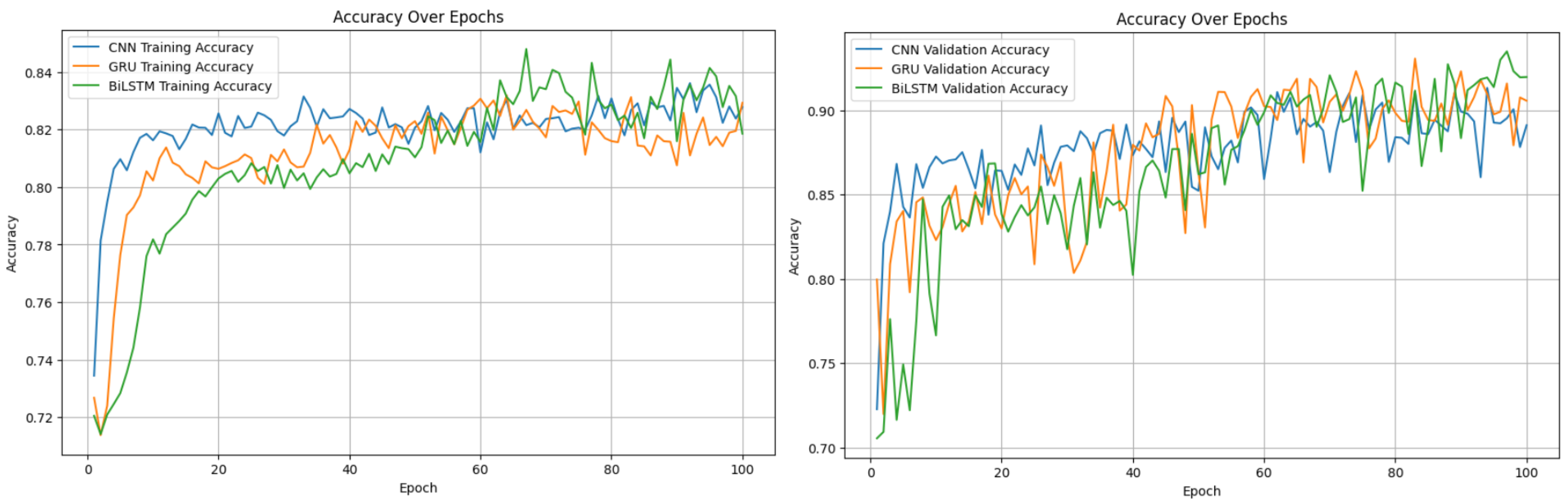
Despite achieving a slight improvement, we aimed for exceptional performance. We sought an approach that would ensure high training and testing accuracy without overfitting, while still delivering reliable predictions when the model was applied. Given the temporal nature of EEG data, where each time segment depends on the previous one, we decided to explore recurrent neural networks (RNNs). Specifically, we implemented a GRU model, a variant of RNN, and a BiLSTM model, a variant of LSTM (which is itself a type of RNN). To assess the comparative performance of convolutional neural networks (CNNs), we implemented a CNN model as well.
For this study, we chose to work with data from six subjects. This number struck a balance: using fewer subjects led to overfitting, while using more made it challenging for the models to perform effectively. The choice of six subjects allowed us to achieve high accuracy without overfitting. The accompanying figures provide a detailed explanation of the results.
Figure 9.
Training and Validation accuracies evaluation.
Figure 9.
Training and Validation accuracies evaluation.
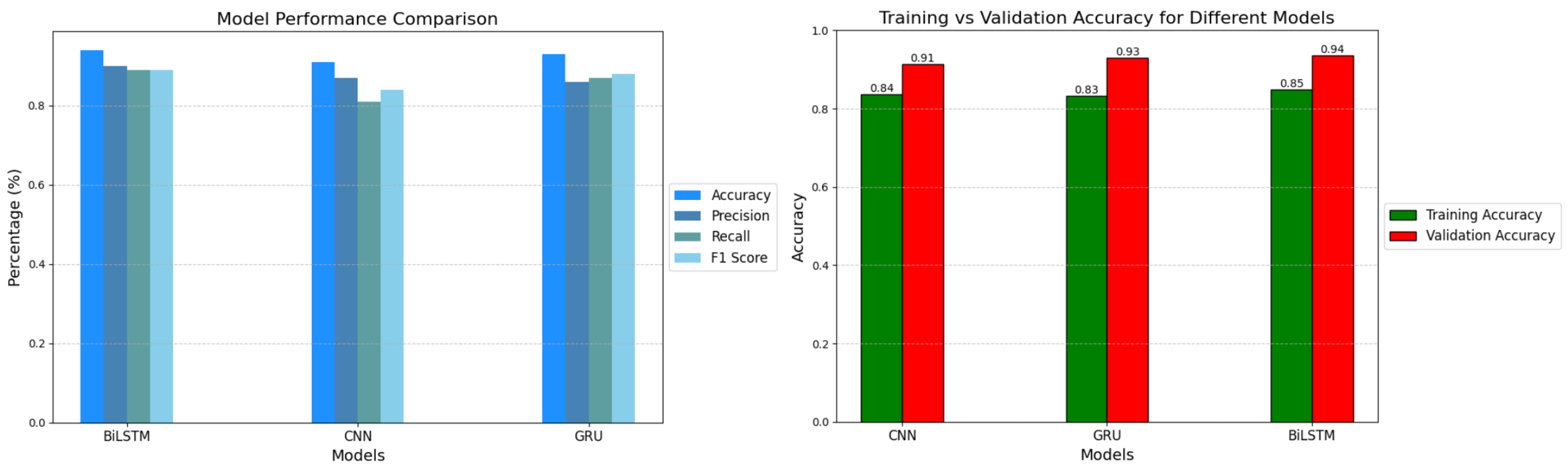
Figure 10.
Models Comparison.
Figure 10.
Models Comparison.
Table 3.
Accuracy comparison of the models.
Table 3.
Accuracy comparison of the models.
| Models |
Training Accuracy |
Testing Accuracy |
| BiLSTM |
85% |
94% |
| GRU |
83% |
93% |
| CNN |
84% |
91% |
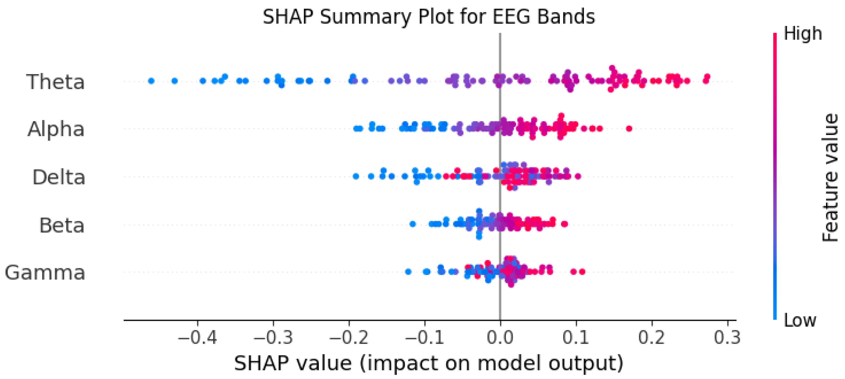
Understanding the reasoning behind the model’s predictions was a key objective of this study. Among all the implemented algorithms, the BiLSTM model consistently delivered the most outstanding performance. To gain insights into how this model generates its predictions and to identify the features driving its decisions, we utilized SHapley Additive exPlanations (SHAP). Through this analysis, we discovered that the features Theta and Alpha had the most substantial influence on the model’s predictions, playing a pivotal role in shaping its diagnostic outcomes. Conversely, the Gamma feature demonstrated minimal impact, indicating its lack of discriminative power in this specific context. This evaluation was based on a detailed analysis of 100 EEG segments, offering a comprehensive understanding of the feature importance and the inner workings of the BiLSTM model.
Figure 11.
SHAP plot of the BiLSTM model.
Figure 11.
SHAP plot of the BiLSTM model.
The primary goal of this project is to enable real-time emotion detection based on EEG signals. Through our research, we determined that a 2-second segment of EEG data is sufficient to accurately identify a person’s emotional state. This insight allowed us to design and implement a real-time application tailored for this purpose.
The application processes EEG data in real time, providing two key outputs: a visual representation of the participant’s EEG signals and the corresponding detected emotional state. The input to the system is a pre-recorded or live EEG file, which is being analyzed using our best model, the BiLSTM, to extract meaningful features and classify the individual’s emotional state. The signal plot offers a clear view of the participant’s neural activity, while the emotion detection output provides an intuitive and immediate understanding of their emotional state.
This real-time capability makes the application particularly valuable in various domains, including mental health monitoring, human-computer interaction, and adaptive learning systems. By bridging neuroscience and machine learning, the tool offers a practical and efficient solution for emotion recognition, emphasizing both accuracy and usability.
Despite all of these, we still know that we can achieve better results, the approachs change form a group to another group, so we know that there’s some architectures, that can achieve magnificient results
6. Conclusions And Future Work
This study establishes the potential of advanced deep learning models for EEG-based emotion classification. Future work will focus on refining some deep learning architectures and exploring real-time implementations for broader applications in neurofeedback and mental health monitoring. Despite these advancements, there remains the opportunity to achieve even better results, as approaches vary across different research groups. Several architectures have demonstrated the capability to achieve remarkable outcomes. Instead of relying solely on EEG data, attention will shift towards integrating additional signals, such as heart rate, respiratory rate, skin conductance, muscle activity, and more. The inclusion of these diverse signals will enhance emotion detection efficiency.
Moreover, significant efforts will be directed towards refining models, employing sophisticated data preprocessing, feature extraction, and advanced machine learning techniques. Additionally, the interpretability of the models will be refined to ensure that the rationale behind predictions is clear, accompanied by a real-time emotion detection system to further support this approach.
References
- Mauss, Iris B and Robinson, Michael D. Measures of emotion: A review. Cognition and emotion 2009, 23, 209–237. Taylor & Francis. [CrossRef]
- Govindaraju, Vimala and Thangam, Dhanabalan, Emotion Recognition in Human-Machine Interaction and a Review in Interpersonal Communication Perspective, Human-Machine Collaboration and Emotional Intelligence in Industry 5.0, 329–343, 2024, IGI Global.
- Lan, Zirui, EEG-based emotion recognition using machine learning techniques, 2018.
- Jerritta, S and Murugappan, M and Nagarajan, R and Wan, Khairunizam, Physiological signals based human emotion recognition: A review, 2011 IEEE 7th international colloquium on signal processing and its applications, 410–415, 2011, IEEE.
- Adolphs, Ralph, Cognitive neuroscience of human social behavior, Neuropsychologia, 41, 119–126, 2003.
- Böcker, Koen BE and van Avermaete, Jurgen AG and van den Berg-Lenssen, Margaretha MC, The international 10–20 system revisited: Cartesian and spherical co-ordinates, Brain Topography, 6, 231–235, 1994, Springer.
- Cowie, Roddy and Douglas-Cowie, Ellen and Tsapatsoulis, Nicolas and Votsis, George and Kollias, Stefanos and Fellenz, Winfried and Taylor, John G, Emotion recognition in human-computer interaction, IEEE Signal processing magazine, 18, 1, 32–80, 2001, IEEE. [CrossRef]
- Cowie, Roddy and Douglas-Cowie, Ellen and Tsapatsoulis, Nicolas and Votsis, George and Kollias, Stefanos and Fellenz, Winfried and Taylor, John G, Emotion recognition in human-computer interaction, IEEE Signal processing magazine, 18, 1, 32–80, 2001, IEEE. [CrossRef]
- Koelstra, Sander and Muhl, Christian and Soleymani, Mohammad and Lee, Jong-Seok and Yazdani, Ashkan and Ebrahimi, Touradj and Pun, Thierry and Nijholt, Anton and Patras, Ioannis, Deap: A database for emotion analysis; using physiological signals, IEEE transactions on affective computing, 3, 1, 18–31, 2011, IEEE. [CrossRef]
- Chen, JX and Zhang, PW and Mao, ZJ and Huang, YF and Jiang, DM and Zhang, YN, Accurate EEG-based emotion recognition on combined features using deep convolutional neural networks, IEEE Access, 7, 44317–44328, 2019, IEEE. [CrossRef]
- Alhagry, Salma and Fahmy, Aly Aly and El-Khoribi, Reda A, Emotion recognition based on EEG using LSTM recurrent neural network, International Journal of Advanced Computer Science and Applications, 8, 10, 2017, Science and Information (SAI) Organization Limited.
- Li, Youjun and Huang, Jiajin and Zhou, Haiyan and Zhong, Ning, Human emotion recognition with electroencephalographic multidimensional features by hybrid deep neural networks, Applied Sciences, 7, 10, 1060, 2017, MDPI. [CrossRef]
- Xing, Xiaofen and Li, Zhenqi and Xu, Tianyuan and Shu, Lin and Hu, Bin and Xu, Xiangmin, SAE+ LSTM: A new framework for emotion recognition from multi-channel EEG, Frontiers in neurorobotics, 13, 37, 2019, Frontiers Media SA. [CrossRef]
- Pichandi, Sivasankaran and Balasubramanian, Gomathy and Chakrapani, Venkatesh, Hybrid deep models for parallel feature extraction and enhanced emotion state classification,Scientific Reports, 14, 1, 24957, 2024, Nature Publishing Group UK London. [CrossRef]
- Chen, JX and Jiang, DM and Zhang, YN, A hierarchical bidirectional GRU model with attention for EEG-based emotion classification, IEEE Access, 7, 118530–118540, 2019, IEEE. [CrossRef]
- Mehrabian, Albert, Pleasure-arousal-dominance: A general framework for describing and measuring individual differences in temperament, Current Psychology, 14, 261–292,1996, Springer. [CrossRef]
- Soleymani, Mohammad and Lichtenauer, Jeroen and Pun, Thierry and Pantic, Maja, A multimodal database for affect recognition and implicit tagging, IEEE transactions on affective computing, 3, 1, 42–55,2011, IEEE. [CrossRef]
- Newson, Jennifer J and Thiagarajan, Tara C, EEG frequency bands in psychiatric disorders: A review of resting state studies, Frontiers in human neuroscience, 12, 521, 2019, Frontiers Media SA. [CrossRef]
- Bigdely-Shamlo, Nima and Mullen, Tim and Kothe, Christian and Su, Kyung-Min and Robbins, Kay A, The PREP pipeline: Standardized preprocessing for large-scale EEG analysis, Frontiers in neuroinformatics, 9, 16, 2015, Frontiers Media SA. [CrossRef]
- Bhole, L and Ingle, M, Estimating range and relationship of EEG frequency bands for emotion recognition, International Journal of Computer Applications, 78, 13, 16–21, 2019. [CrossRef]
- Mendivil Sauceda, Jesus Arturo and Marquez, Bogart Yail and Esqueda Elizondo, José Jaime, Emotion Classification from Electroencephalographic Signals Using Machine Learning, Brain Sciences, 14, 12, 1211, 2024, MDPI.
- Unde, Sukhada A and Shriram, Revati, Coherence analysis of EEG signal using power spectral density, 2014 Fourth International Conference on Communication Systems and Network Technologies, 871–874, 2014, IEEE.
- Dwivedi, Amit Kumar and Verma, Om Prakash and Taran, Sachin, 2024 11th International Conference on Signal Processing and Integrated Networks (SPIN), EEG-Based Emotion Recognition Using Optimized Deep-Learning Techniques, 2024, , , 372-377, Deep learning;Time-frequency analysis;Emotion recognition;Computational modeling;Brain modeling;Feature extraction;Electroencephalography;EEG;Emotion Recognition;Deep-Learning Methods;Bayesian Optimization, 10.1109/SPIN60856.2024.10512074.
- Tong, Wenhui and Yang, Li and Qin, Yingmei and Che, Yanqiu and Han, Chunxiao, 2022 15th International Congress on Image and Signal Processing, BioMedical Engineering and Informatics (CISP-BMEI), EEG-Based Emotion Recognition by Using Machine Learning and Deep Learning, 2022, , ,1-5, Deep learning;Radio frequency;Emotion recognition;Machine learning algorithms;Support vector machine classification;Signal processing algorithms;Forestry;EEG;emotion;support vector machine(SVM);random forest(RF);convolutional neural network(CNN), 10.1109/CISP-BMEI56279.2022.9979849.
- Li, Xiang and Zhang, Yazhou and Tiwari, Prayag and Song, Dawei and Hu, Bin and Yang, Meihong and Zhao, Zhigang and Kumar, Neeraj and Marttinen, Pekka, EEG based emotion recognition: A tutorial and review, ACM Computing Surveys, 55, 4, 1–57, 2022, ACM New York, NY. [CrossRef]
- Gramfort, Alexandre and Luessi, Martin and Larson, Eric and Engemann, Denis A and Strohmeier, Daniel and Brodbeck, Christian and Parkkonen, Lauri and Hämäläinen, Matti S, MNE software for processing MEG and EEG data, neuroimage, 86, 446–460, 2014, Elsevier. [CrossRef]
- Ma, Yahong and Huang, Zhentao and Yang, Yuyao and Zhang, Shanwen and Dong, Qi and Wang, Rongrong and Hu, Liangliang, Emotion Recognition Model of EEG Signals Based on Double Attention Mechanism, Brain Sciences, 14, 12, 1289, 2024, MDPI. [CrossRef]
- Jacob12138xieyuan, EEG-Based Emotion Recognition on DEAP, https://github.com/Jacob12138xieyuan/EEG-Based-Emotion-Recognition-on-DEAP.
|
Disclaimer/Publisher’s Note: The statements, opinions and data contained in all publications are solely those of the individual author(s) and contributor(s) and not of MDPI and/or the editor(s). MDPI and/or the editor(s) disclaim responsibility for any injury to people or property resulting from any ideas, methods, instructions or products referred to in the content. |
© 2025 by the authors. Licensee MDPI, Basel, Switzerland. This article is an open access article distributed under the terms and conditions of the Creative Commons Attribution (CC BY) license (http://creativecommons.org/licenses/by/4.0/).