
Submitted:
08 August 2025
Posted:
11 August 2025
You are already at the latest version
Abstract
Several chemistry-climate models (CCM) tend to underestimate the total column ozone (TCO) over the southern polar region during winter. The most significant discrepancies were found in the CCM SOCOLv3, which we utilize to study the sensitivity of TCO over Antarctica to the following key influencing factors: (1) the efficiency of stratospheric heterogeneous reactions, (2) the intensity of meridional flux into the polar regions due to sub-grid scale mixing processes, and (3) the accuracy of photodissociation rate calculations. Comparisons of the model results with satellite observations from IKFS-2, MLS, and MIPAS showed that the most effective processes for improving polar ozone simulation are photolysis and horizontal mixing. An increase in horizontal mixing improves the simulated TCO seasonal cycle; however, it negatively impacts the representation of the CH4 and N2O distributions. The application of the photolysis module Cloud-J v.8.0 has improved the accuracy of photolysis rate calculations and the representation of the seasonal ozone cycle over the southern polar region. This paper outlines the impact of various processes on the performance of chemistry-climate models in the southern polar stratosphere, with potential implications for future advancements in this area.
Keywords:
ozone layer
; chemistry-climate models
; stratospheric chemistry
; horizontal transport
; photolysis rate
1. Introduction
The atmospheric ozone (O3) layer is an essential factor for the sustainability of the Earth's biosphere and human health. It shields all living organisms from the Sun's harmful ultraviolet radiation in the UV-C and UV-B bands of the solar spectrum. Additionally, as a radiatively active gas, ozone contributes substantially to the energy balance of the Earth [1].
Stratospheric ozone has been depleting since the 1970s due to emissions of chlorine and bromine-containing substances. In the 1980s, the ozone hole was discovered in the Southern Hemisphere at high-latitude polar station [2]. In response, governments around the world signed the Montreal Protocol to limit the production of chlorofluorocarbons (CFCs), which came into force in 1989. To assess the effectiveness of the Protocol and to understand the atmospheric ozone evolution in the 21st century, a special class of models known as Chemistry-Climate models (CCM) has been applied [3]. CCM considers the main processes responsible for the ozone layer state and enables calculations of the fundamental characteristics of the Earth's atmospheric circulation [4,5,6].
Usually, the CCM performance at the high latitudes has been evaluated only for the periods when solar light is available. Studies have shown that many models perform well over the southern high latitudes in early spring [6,7,8]. The lack of model validation during the polar night is because, until 2014, most satellite instruments could not measure the ozone in the polar latitudes of the Southern Hemisphere because of the absence of solar light. The only TOVS (The TIROS Operational Vertical Sounder) satellite instrument has performed measurements of TCO during the polar night, but its relative measurement error was too high [9]. The situation changed with the introduction of spectrometers that operate in the infrared range. One such device is the Infrared Fourier Spectrometer (IKFS-2), which provides data on the ozone content under both night and day conditions with an accuracy of 5% [10].
Figure 1 illustrates the climatological annual cycle of TCO (in Dobson Units or DU) averaged over 75-80°S from satellite measurements with IKFS-2 and SBUV sensors together with the results of SOCOLv3, CMAM, MIROC 3.2, NIWA-UKCA, GEOSCCM, MRI-ESM, and ULAQ chemistry-climate models. SBUV data were acquired from https://acd-ext.gsfc.nasa.gov/Data_services/merged. The model data were acquired from the CCMI-1 data archive (https://data.ceda.ac.uk/badc/wcrp-ccmi/data/CCMI-1). The SOCOLv3 data for 2014-2018 were produced using the CCM SOCOLv3 version used in CCMI-1.
The figure shows a good agreement between SBUV and IKFS2 data during the austral spring and summer seasons (October-February), when the SBUV data are available. The comparison of SOCOLv3 data from 1990-2009 and 2014-2018 indicates minor changes in TCO behavior during autumn and winter. It is evident that all CCMs tend to underestimate polar TCO values from April to July. Among these, the GEOSCCM exhibits the smallest deviation, while SOCOLv3 shows the largest error (~100 DU) compared to the IKFS-2 data. From October to December, SOCOLv3, GEOSCCM, MRI-ESM, and ULAG align with the IKFS-2 data within the uncertainty range, whereas MIROC3.2, CMAM, and NIWA-UKCA demonstrate some underestimation. Consequently, the TCO levels in October, often used for evaluating model performance in simulating the ozone hole, do not provide comprehensive information about model quality. The polar night area is particularly noteworthy because virtually all models indicate lower TCO compared to satellite data. The reasons behind this TCO underestimation are currently unknown, presenting a significant gap in our understanding of the processes that define the state of the ozone layer. In this study, we aim to improve the representation of the southern polar TCO in the CCM SOCOLv3, as we have full access to this model, where the issues are most significant. We considered several factors that affect the annual cycle of polar ozone in the Southern Hemisphere: (1) the efficiency of the heterogeneous reactions; (2) the intensity of the sub-grid-scale meridional mixing (into the polar vortexes), and (3) the accuracy of the photolysis rate calculations for the large solar zenith angles. To evaluate the impact of photolysis rates for large solar zenith angles, we applied a new version of CCM SOCOLv3 that incorporates the Cloud-J v.8.0 module for the photolysis rate calculation [11].
2. Materials and Methods
2.1. Data Used for Comparison
To compare model data on TCO with actual observations, we used data from the IKFS-2 instrument, which is installed on the «Meteor-M N2» series satellite. This instrument is designed to measure the spectra of outgoing radiation from the atmosphere-surface system, essential for obtaining various types of information, including temperature and humidity profiles, total ozone content, surface temperature, fraction of cloud cover, and pressure at the upper cloud boundary. The purpose, design and main characteristics of IKFS-2 are presented in [10]. The study in [12] analyzes the operation of IKFS-2, including an assessment of measurement quality (errors in radiometric and spectral calibration) and their information content. The TCO processing algorithms are described in [13]. The data IKFS-2 has been available since March 2015 and for our comparison, we focused on data collected during the period from 2016 to 2020.
To compare the simulated vertical profiles of O3, N2O, and CH4 we utilized two different instruments: the Microwave Limb Sounder (MLS) on board NASA's Aura satellite and the Michelson Interferometer for Passive Atmospheric Sounding (MIPAS). MLS measures microwave thermal radiation from the limb of the atmosphere using seven radiometers [14]. The instrument provides vertical profiles of atmospheric components with high spatial coverage. MIPAS is a mid-infrared emission spectrometer that is part of the core payload of ENVISAT. It is a limb sounder, i.e. it scans across the horizon, detecting atmospheric spectral radiances which are then inverted to derive vertical temperature, trace species, and cloud distributions. [15]. For our analysis, we use MLS data for the period 2014 - 2018 and MIPAS data for 2008-2012.
2.2. Cloud-J v.8.0
Cloud-J v.8.0 is a broadband algorithm designed for calculating photolysis rates in the presence of cloud and aerosol layers. This algorithm enables the simulation of global atmospheric photochemistry by directly incorporating the physical properties of scattering and absorbing particles. The radiative transfer calculations in Cloud-J v.8.0 are based on the Feautrier method for solving the radiative transport equations in a plane-parallel atmosphere. The Cloud-J v.8.0 spectral range (177.5–778 nm) is divided into 18 spectral intervals (bins). Spectral data (absorption cross sections and dissociation quantum yields) are calculated based on laboratory data, in particular, JPL and IUPAC [16,17].
A complete set of equations, a description of the methods for accounting for processes associated with the passage of solar radiation, and a detailed description of the spectral range can be found in [11,18]. Comparison of data obtained by Cloud-J v.8.0 and libRadtran [19], as well as the sensitivity of the module to the atmospheric parameters, is presented in the paper [20].
The photolysis rates in SOCOLv3 are calculated using the lookup-table method (LUT) [21]. In the case of large zenith angles of the Sun, spherical geometry is included in the model calculation of the photolyze rates. This approach provides the not-zero photodissociation values even when the solar zenith angle exceeds 90°, but the accuracy of this addition to the LUT scheme was not qualified.
The new photolysis rate calculation module Cloud-J v.8.0 includes solar flux calculations for solar zenith angles > 90°, considering spherical raytracing, extinction of the direct solar beam, and a true geometric atmosphere instead of a flat geopotential atmosphere used in most models [22], which facilitates more accurate calculation of photolysis rates.
2.3. CCM SOCOLv3
The CCM SOCOLv3 calculates various atmospheric dynamic processes interactively, including the hydrological cycle, cloud formation, convection, solar and thermal radiation fluxes, photolysis, chemical transformations, and vertical and horizontal transport of species. The main components of the model are illustrated in Figure 2.
The CCM SOCOLv3 consists of the general circulation model (GCM) of the middle atmosphere ECHAM5 and the chemical module (CM) MEZON. GCM and CM are interactively linked through 3D fields of temperature, winds (from GCM to CM), as well as radiatively active species such as water vapor, ozone, methane, nitrous oxide, and chlorofluorocarbons (from CM to GCM). The model includes 41 chemical elements from the groups of oxygen, hydrogen, nitrogen, carbon, chlorine, and bromine. Interactions between gas species are determined by 140 gas phase reactions, 46 photolysis reactions, and 16 heterogeneous reactions on liquid sulfate aerosols and solid particles of water ice and nitric acid trihydrate [23]. As external drivers of the atmospheric state, the model can use greenhouse gases and ozone-depleting substances mixing ratios, sea surface temperature (SST) and sea ice concentration (SIC), spectral solar radiation, sulfate aerosols properties, and some other parameters.
To calculate photolysis rates in SOCOLv3, the default LUT method is used. For one model run, we installed the Cloud-J v.8.0 module, which receives solar irradiance and atmospheric parameters from ECHAM5 and MEZON and then feeds the calculated rates back to MEZON.
The SOCOLv3 has 39 vertical levels (from the surface up to 0.01 hPa) and has been used with a horizontal resolution of T42. The model can be run very efficiently in parallel mode.
2.4. Description of the Model Runs
2.4.1. Reference Run (RR)
To compare the original calculation results of the CCM SOCOLv3 with the IKFS-2 measurements, we have conducted a 19-year-long reference numerical experiment for the 2000-2018 period. The first 14 years (2000-2013) of the model calculations were considered as a spin-up period, which is essential for the adaptation of the model’s atmospheric chemical composition and dynamics to the specific boundary conditions. The last 5 years of the model experiment (2014-2018) were used for analysis and comparison with the corresponding IKFS-2 observations.
As boundary conditions, we considered the long-term (2000-2018) evolution of the ozone-depleting substances (ODS), greenhouse gas concentrations (GHG), sea surface temperature and sea ice concentration (SST/SIC), and zonal winds in the equatorial stratosphere (QBO). The mixing ratios of ODS in the lower troposphere were based on the data from the World Meteorological Organization (WMO) [25]. The atmospheric mixing ratios for the primary GHG (CO2, CH4, and N2O) are taken from [26] until 2014 and extended to 2018 following the IPCC SSP2-4.5 scenario [27].
The SST/SIC fields for the 21st century, prescribed as monthly means, are adopted from the HadISST1 dataset provided by the UK Met Office Hadley Centre [28]. The QBO is produced by a linear relaxation (“nudging”) of the model zonal winds in the equatorial stratosphere to a time series of observed winds [29]. The nudging is used between 20o N and 20o S from 90 hPa up to 3 hPa. Within the QBO core domain (10o N–10o S, 50– 8 hPa), the relaxation time is uniformly set to 7 days; outside this region, the damping depends on latitude and altitude [30]. Also, the evolutions of the 11-year solar activity [31], stratospheric aerosol contents [32], and the surface CO and NOx emissions from CMIP6 input4MIPs databases for the historical period to 2014 and following RCP2-4.5 until 2018 [33] were applied in the model runs as boundary conditions.
2.4.2. Sensitivity Runs (SR1, SR2, SR3)
The TCO discrepancies between model and satellite data (Figure 1) can likely be attributed to inadequate model representations of the processes influencing the polar ozone formation. According to the modern scientific paradigm, the ozone content in the polar stratosphere is controlled mainly by the rates of the heterogeneous reactions and the photodissociation of ozone molecules by solar radiation at the large zenith angles of the Sun [34]. Also, the level of TCO inside the inner part of the SH polar night vortex can depend on the horizontal resolution of the model [35]. So, if the model grid is coarse, it becomes essential to account for the transport of model species into the polar night vortex through the sub-grid scale motions.
Therefore, to investigate the reasons behind the simulated TCO underestimation and improve the accuracy of the model, we performed a set of additional numerical experiments using CCM SOCOLv3, described in Table 1. All these model experiments were set up exactly as the reference case, maintaining the same boundary conditions, spin-up processes, and using model results from the years 2014 to 2018 for comparison with satellite data.
3. Results
Figure 3 illustrates the TCO calculated in the reference run of SOCOLv3 and the corresponding values of TCO obtained from IKFS-2 observations. The figure indicates that the model significantly underestimated the TCO values in the polar region of the SH compared to the satellite data. In August the difference exceeds 90 DU.
3.1. Sensitivity to Heterogeneous Chemistry (SR1)
Chemical reactions on/in polar stratospheric cloud particles play a crucial role in the formation of the Antarctic ozone hole [36]. To analyze the model TCO sensitivity to the intensity of heterogeneous processes, we reduced the rate of the most important heterogeneous reaction HCl + ClONO2 → Cl2 + HNO3, by a factor of two. This reaction is the primary source of the Cl2, which in turn produces active chlorines that destroy polar stratospheric ozone in a photo-catalytic cycle following the polar sunrise.
Figure 4 shows the annual variability of monthly mean TCO at 800S averaged from 2016 to 2018, based on experiments together with the corresponding values from the reference run and the IKFS-2 measurements.
As expected, reduced efficiency of the HCl + ClONO2 → Cl2 + HNO3 reaction rate leads to smaller ozone depletion and higher TCO only from October to December. However, this rate correction does not significantly impact TCO values within the polar vortex during the polar night and does not play a substantial role during winter.
3.2. Sensitivity to the Subgrid-Scale Mixing (SR2)
Previous numerical experiments using chemistry-transport models provided some evidence that the air mass exchange between the polar vortex area and the middle latitude in the SH stratosphere depends on the applied horizontal resolution [35,37]. The calculated mass fluxes into the inner region of the vortex from outside increase when the model's horizontal resolution is higher. It can be explained by the fact that the model with the higher horizontal resolution generates additional transport by the atmospheric motions that cannot be resolved by the model with the coarse grid.
To verify this suggestion for SOCOLv3, we included in the model’s lower stratosphere a zonally averaged meridional diffusion of the species with a coefficient Kyy which depends only on time and latitude. According to the Prandl mixing length theory, the maximum values of Kyy can be estimated as < 6·106 m2/s (mixing length < 3·105 m and meridional wind variations < 20 m/s on the model meridional grid scale (~ 2.50)). We suggest also that the Kyy reached its maximum in the areas of the polar vortex locations. The time-latitudinal mask for the Kyy values is presented in Figure 5.
To evaluate the sensitivity of the model calculations to the intensity of the suggested diffusion process, a set of model runs was undertaken with Kyy varying from 3·105 m2/s to 6·106 m2/s in its maximum. The most visible result was obtained in the run with the maximum value of Kyy=5·106 m2/s (run SR2).
The monthly mean TCO for ~800S from SR2 together with the corresponding TCO data from the other experiments (RR, SR1, SR3) and IKFS-2 observations are presented in Figure 4 which demonstrates that enhancement of the subgrid-scale mixing process in the model leads to a remarkable decrease in the TCO bias of CCM SOCOLv3 in comparison with the results of the satellite measurements. Therefore, it could be expected that this very simplified approach can be useful for the CCMs with a coarse horizontal grid (>10).
However, the enhancement of the horizontal mixing into southern high latitudes for the SR2 experiment also affects the vertical distribution of other atmospheric species in these regions. To estimate this effect, we compared the vertical profiles of the mixing ratios of the simulated CH4, N2O, and O3 over the south polar region in August with the MIPAS and MLS measurements. Figure 6 shows the results of this comparison for the RR (upper panels: a, b, and c) and SR2 (lower panels: d, e, and f) experiments. The differences in the model ozone mixing ratio in comparison with the MLS data are shown in panels a and d, the differences in the model CH4 mixing ratio relative to the MIPAS data in panels b and e, and the differences in the model N2O concentrations relative to the MLS data in panels c and f, respectively. The analysis of the results shows that in the lower stratosphere over Antarctica, the deviation of the O3 concentrations calculated in the SR2 experiment from the MLS data (d) changes sign and significantly exceeds the absolute value of the corresponding deviations in the RR experiment (a) leading to an improvement in TCO values. In the lower polar stratosphere, the errors of the model methane and nitrous oxide concentrations relative to the measurement data from the MIPAS and MLS instruments in the SR2 experiment (e and f) are significantly larger than the corresponding errors in the RR numerical experiment (b and c). This discrepancy arises because Prandtl's theory provides an approximate estimate of possible values for Kyy. As a result, the value of Kyy we selected, optimal for approximating the TCO values from the SR2 experiment to the IKFS-2 data and introduces significant distortions into the corresponding model vertical profiles of the CH4, N2O, and O3 concentrations when compared to the RR experiment. Thus, we conclude that the failure to consider the subgrid-scale mixing processes in our RR experiment is not the main source of the computed TCO errors in the southern polar region for the SOCOLv3 model.
3.3. Improved Photodissociation Rate Calculations Module (SR3)
Another possible cause of the problem may relate to the accuracy of the photodissociation rate calculations, which we derived using a simple lookup table (LUT) approach. To calculate the photolysis rates in this model run, we coupled the Cloud-J v.8.0 to CCM SOCOLv3. However, since the spectral range of Cloud-J v.8.0 is limited to 177.5–778 nm and does not allow considering gas components, in which photodissociation occurs at shorter wavelengths, such as O2(O+O(1D), H2O, and CH4. Therefore, we calculate the photolysis rates for these gases using the LUT scheme.
Figure 7 shows the absolute difference in total ozone content between the reference run and the model run with Cloud-J v.8.0, compared to the data IKFS-2. It is shown that the use of Cloud-J v.8.0 for calculating photolysis rates improves the modeling of TCO over the southern polar region from June to September. The difference in TCO between the reference run and satellite data in July was 80 DU, in the model run using Cloud-J v.8.0, the difference decreased to 40 DU.
To analyze the changes in the simulated atmosphere, we compare photolysis rates and atmospheric chemistry response to the changes in the photolysis rate calculation method.
Figure 8 shows the photolysis rates of O2 and O3(total) on the edge of the vortex during the polar night for a zenith angle of 93°, calculated using LUT and Cloud-J + LUT. It is shown that the rates of oxygen photolysis calculated using Cloud-J + LUT are higher than those calculated with only LUT, while the rates of ozone photolysis, on the contrary, are lower.
The differences in the photolysis rates can affect ozone content in three different ways. Higher molecular oxygen photolysis (O2+hv=>O+O) can lead to slightly enhanced ozone production via O+O2+M=>O3+M. Lower ozone photolysis can directly enhance O3 concentration. Weaker production of excited atomic oxygen via O3+hv=>O2 + O(1D) or O(3P) can lead to the redistribution of the active radicals from chlorine (ClOx), hydrogen (HOx), and nitrogen (NOx) groups. The model does not show substantial changes in HOx and NOx; however, for the ClOx family, the changes are substantial. They are demonstrated in Figure 9, which shows a significant decrease of OH and O(1D) and transfer of active chlorines (Cl+ClO+HOCl+CL2+Cl2O2) to a more passive HCl form. This process is related to slower HCl destruction by hydroxyl and atomic oxygen via HCl+OH and HCl+O.
Differences in the mixing ratios of O3 between reference run (a), SR2 run (b), and MLS data for the Southern Hemisphere (45-80°S) averaged over the 2014-2018 period are presented in Figure 10.
The application of the new photolysis module improves the agreement between model results and MLS data in the entire stratosphere during the winter. The underestimation of the ozone mixing ratio remains above 10 hPa, but its magnitude is substantially smaller during June and July and almost insignificant in August. In the lower stratosphere (below 10 hPa), the improvement is the most pronounced during July and August. During these months, the previously simulated substantial negative bias vanishes over high latitudes, with remaining positive biases considerably diminished north of 60°S.
Figure 11 illustrates differences in the mixing ratios of CH4 and N2O between the reference experiment (a), SR2 experiment (b), and MLS and MIPAS data. It indicates that, unlike the results from the SR2 experiment, the deviations in the vertical profiles of methane and nitrous oxide from observed values remain consistent. The significant positive biases in the simulated data remain virtually the same, likely due to an underestimation of the downward transport within the polar vortex.
4. Discussion
The availability of high-quality satellite measurements by infrared-based satellite instruments (e.g. IKFS-2) has significantly enhanced the evaluation of the CCM's performance over polar regions, especially under polar night conditions. Comparison of the TCO simulation results by the CCM SOCOv3 and other CCMs with the satellite data revealed the existence of too-low values of the model TCO during the polar night inside the southern vortex. The causes of the identified problem were not indicated in the available publications. To address this, we exploit the CCM SOCOLv3 to quantify the sensitivity of the total column ozone over Antarctica to (1) the efficiency of stratospheric heterogeneous reactions, (2) the intensity of the meridional flux into the polar regions due to sub-grid scale mixing processes, and (3) the accuracy of photodissociation rate calculations. Our comparisons of modeling results with corresponding satellite measurements indicate that the efficiency of heterogeneous reactions plays only a minor role during the polar winter. The most important process for improving the simulated polar ozone levels is the accuracy of the photolysis rate calculations at the large zenith angles and the intensity of horizontal mixing into the polar vortices. Increasing the intensity of horizontal mixing significantly improves the simulated TCO seasonal cycle. However, it also negatively impacts the representation of the CH4 and N2O distributions, enhancing the positive bias compared to the MLS and MIPAS observations in the original model version.
The application of the photolysis module Cloud-J v.8.0 allowed for an increase in the accuracy of photolysis rate calculations, thereby improving the representation of the seasonal ozone cycle in the southern polar region. As a result, the TCO difference compared to the IKFS-2 measurements has reduced from over 100 to approximately 40 DU in the Southern Hemisphere.
The model performance at the middle latitudes remains virtually the same, suggesting that the improvements are specifically due to more accurate photolysis rate calculations for high zenith angles. The positive bias in CH4 and N2O concentrations is not sensitive to these photolysis rate calculations. This fact, together with the remaining negative bias in the lower stratospheric ozone, inspires further studies to elucidate possible problems with some other processes. One possible explanation could be related to the underestimation of the intensity of simulated downward transport, which moves air masses with a lower mixing CH4 and N2O ratio and higher ozone content from the middle and upper stratosphere.
In summary, this paper discusses the impact of different processes on the effectiveness of chemistry-climate models in simulating the total ozone in the southern polar atmosphere. By examining factors such as stratospheric heterogeneous reactions, meridional flux intensity, and the accuracy of photodissociation rate calculations, the study identifies critical mechanisms that affect ozone distribution. The insights gained from these findings possess significant implications for the refinement of CCMs, potentially leading to a deeper understanding of ozone layer evolution in response to climate change scenarios and policy interventions.
Author Contributions
Conceptualization, E.R. V.Z. A.I. and T.E.; methodology V.Z. and E.R.; software, A.I. V.Z. G.N. A.P. and A.M.; formal analysis, A.I. V.Z, A.M. E.R. and T.E.; resources, E.R.; data curation, A.I, V.Z. G.N. A.P.; writing—original draft preparation, A.M.; writing—review and editing, A.I. V.Z, A.M. E.R. and T.E.; visualization, A.I. A.M. V.Z. and E.R.; supervision, E.R.; project administration, E.R.; funding acquisition, E.R. All authors have read and agreed to the published version of the manuscript.
Funding
The work of A.I. E.R. V.Z. A.P. A.M. and G.N. on the model experiments, preparation of the observation data, analysis of the results, and writing of the manuscript was supported by St. Petersburg State University under research grant 124032000025-1. The work of A.I. on numerical tests of the photolysis algorithm was carried out within the framework of the State Task of the Ministry of Science and Higher Education of Russia for the Russian State Hydrometeorological University (project FSZU-2023-0002). The work of T.E. was supported by the Swiss National Science Foundation project 200021L-22814 10001350 (STOA).
Data Availability Statement
The datasets presented and discussed in this study can be found in online repositories https://doi.org/10.5281/zenodo.16062571
Acknowledgments
Model simulations have been performed on the SPBU cluster. We acknowledge the help of A. Divin and A. Zarochentsev with the model maintenance and execution.
Conflicts of Interest
The authors declare no conflict of interest. The funders had no role in the design of the study; in the collection, analyses, or interpretation of data; in the writing of the manuscript; or in the decision to publish the results.
References
- Bernhard, G.H.; Neale, R.E.; Barnes PW, et, a. l. Environmental effects of stratospheric ozone depletion, UV radiation and interactions with climate change: UNEP Environmental Effects Assessment Panel, update 2019. Photochem Photobiol Sci 2020, 19, 542. [Google Scholar] [CrossRef] [PubMed]
- Farman, J.; Gardiner, B.; Shanklin, J. Large losses of total ozone in Antarctica reveal seasonal ClOx/NOx interaction. Nature 1985, 315, 207–210. [Google Scholar] [CrossRef]
- Egorova, T.; ERozanov Gröbner J, Hauser M, Schmutz, W. Montreal Protocol benefits simulated with CCM SOCOL. Atmos. Chem. Phys. 2013, 13, 3811–3823. [Google Scholar] [CrossRef]
- SPARC, 2010: SPARCCCMVal Report on the Evaluation of Chemistry-Climate Models, V. SPARC; 2010: SPARCCCMVal Report on the Evaluation of Chemistry-Climate Models, V. Eyring, T. Shepherd and D. Waugh (Eds.), SPARC Report No. 5, WCRP-30, 2010, WMO/TD – No. 40, available at www.sparc-climate.
- Eyring, V.; Chipperfield, M.; Giorgetta, M.; et al. Overview of the New CCMVal Reference and Sensitivity Simulations in Support of Upcoming Ozone and Climate Assessments and the Planned SPARC CCMVal, SPARC Newsletter No. 30, 2008, 20–26. https://www.atmosp.physics.utoronto.ca/SPARC/Newsletter30Web/53294-1%20SPRAC%20Newsletter-LR.pdf.
- Dhomse, S.S.; Kinnison, D.; Chipperfield, M.P.; et al. Estimates of ozone return dates from Chemistry-Climate Model Initiative simulations. Atmos. Chem. Phys. 2018, 18, 8409–8438. [Google Scholar] [CrossRef]
- Siddaway, J.M.; Petelina, S.V.; Karoly, D.J.; Klekociuk, A.R.; Dargaville, R.J. Evolution of Antarctic ozone in September–December predicted by CCMVal-2 model simulations for the 21st century. Atmos. Chem. Phys. 2013, 13, 4413–4427. [Google Scholar] [CrossRef]
- Karpechko, A.Y.; Maraun, D.; Eyring, V. Improving Antarctic total ozone projections by a process-oriented multiple diagnostic ensemble regression. J. Atmos. Sci. 2013, 70, 3959–3976. [Google Scholar] [CrossRef]
- Corlett, G.K.; Monks, P.S. A comparison of total ozone values derived from the Global Ozone Monitoring Experiment (GOME), the Tiros Operational Vertical Sounder (TOVS) and the Total Ozone Mapping Spectrometer (TOMS). J. Atmos. Sci. 2001, 58, 1103–1116. [Google Scholar] [CrossRef]
- Golovin, Y.M.; Zavelevich, F.S.; Nikulin, A.G.; Kozlov, D.A.; Monakhov, D.O.; Kozlov, I.A.; Arkhipov, S.A.; Tselikov, V.A.; Romanovskii, A.S. Spaceborne Infrared Fourier-Transform Spectrometers for Temperature and Humidity Sounding of the Earth’s Atmosphere. Izv. Atmos. Ocean. Phys. 2014, 50, 1004–1015. [Google Scholar] [CrossRef]
- Wild, O.; Zhu, X.; Prather, M.J. Fast-J: Accurate Simulation of In- and Below-Cloud Photolysis in Tropospheric Chemical Models. J. Atmos. Chem. 2000, 37, 245–282. [Google Scholar] [CrossRef]
- Timofeyev, Y.M.; Uspensky, A.B.; Zavelevich, F.S.; Polyakov, A.V.; Virolainen, Y.A.; Rublev, A.N.; Kukharsky, A.V.; Kiseleva, J.V.; Kozlov, D.A.; Kozlov, I.A.; et al. Hyperspectral infrared atmospheric sounder IKFS-2 on “Meteor-M” No. 2—Four years in orbit. J. Quant. Spectrosc. Radiat. Transf. 2019, 238, 106579. [Google Scholar] [CrossRef]
- Polyakov, A.; Virolainen, Y.; Nerobelov, G.; Kozlov, D.; Timofeyev, Y. Six Years of IKFS-2 Global Ozone Total Column Measurements. Remote Sens. 2023, 15, 2481. [Google Scholar] [CrossRef]
- Waters, J.W.; Froidevaux, L.; Harwood, R.S.; Jarnot, R.F.; Pickett, H.M.; Read, W.G.; Siegel, P.H.; Cofield, R.E.; Filipiak, M.J.; Flower, D.A.; Holden, J.R.; Lau, G.K.; Livesey, N.J.; Manney, G.L.; Pumphrey, H.C.; Santee, M.L.; Wu, D.L.; Cuddy, D.T.; Lay, R.R.; Loo, M.S.; Perun, V.S.; Schwartz, M.J.; Stek, P.C.; Thurstans, R.P.; Chandra, K.M.; Chavez, M.C.; Chen, G.; Boyles, M.A.; Chudasama, B.V.; Dodge, R.; Fuller, R.A.; Girard, M.A.; Jiang, J.H.; Jiang, Y.; Knosp, B.W.; LaBelle, R.C.; Lam, J.C.; Lee, K.A.; Miller, D.; Oswald, J.E.; Patel, N.C.; Pukala, D.M.; Quintero, O.; Scaff, D.M.; Snyder, W.V.; Tope, M.C.; Wagner, P.A.; Walch, M.J. The Earth Observing System Microwave Limb Sounder (EOS MLS) on the Aura satellite. IEEE Trans. Geosci. Remote Sens. 2006, 44, 1075–1092. [Google Scholar] [CrossRef]
- Fischer, H.; Birk, M.; Blom, C.; Carli, B.; Carlotti, M.; von Clarmann, T.; Delbouille, L.; Dudhia, A.; Ehhalt, D.; Endemann, M.; Flaud, J.M.; Gessner, R.; Kleinert, A.; Koopman, R.; Langen, J.; López-Puertas, M.; Mosner, P.; Nett, H.; Oelhaf, H.; Perron, G.; Remedios, J.; Ridolfi, M.; Stiller, G.; Zander, R. : MIPAS: an instrument for atmospheric and climate research, Atmos. Chem. Phys. 2008, 8, 2151–2188. [Google Scholar] [CrossRef]
- Burkholder, J.B.; Sander, S.P.; Abbatt, J.; Barker, J.R.; Huie, R.E.; Kolb, C.E.; Kurylo, M.J.; Orkin, V.L.; Wilmouth, D.M.; Wine, P.H. Chemical Kinetics and Photochemical Data for Use in Atmospheric Studies, Evaluation No. 18, JPL Publication 15-10, Jet Propulsion Laboratory, Pasadena, 2015. Available online: http://jpldataeval.jpl.nasa.gov (accessed on 18 July 2025).
- Atkinson, F.S.; Foster-Powell, K.; Brand-Miller, J.C. International tables of glycemic index and glycemic load values: 2008. Diabetes Care 2008, 31, 2281–2283. [Google Scholar] [CrossRef]
- Bian, H.; Prather, M.J. Fast-J2: Accurate Simulation of Stratospheric Photolysis in Global Chemical Models. J. Atmos. Chem. 2002, 41, 281–296. [Google Scholar] [CrossRef]
- Mayer, B.; Kylling, A. Technical note: The libRadtran software package for radiative transfer calculations - description and examples of use. Atmos. Chem. Phys. 2005, 5, 1855–1877. [Google Scholar] [CrossRef]
- Imanova, A.; Rozanov, E.; Smyshlyaev, S.; Zubov, V.; Egorova, T. Investigation of the Influence of Atmospheric Scattering on Photolysis Rates Using the Cloud-J Module. Atmosphere 2025, 16, 58. [Google Scholar] [CrossRef]
- Rozanov, E.; Zubov, V.; Schlesinger, M.; Yang, F.; Andronova, N. The UIUC 3-D Stratospheric Chemical Transport Model: Description and Evaluation of the Simulated Source Gases and Ozone. J. Geophys. Res. 1999, 104, 11755–11781. [Google Scholar] [CrossRef]
- Prather, M. ; JC Hsu, A round Earth for climate models. Proc. Natl. Acad. Sci. 2019, 116, 19330–19335. [Google Scholar] [CrossRef]
- Stenke, A.; Schraner, M.; Rozanov, E.; Egorova, T.; Luo, B.; Peter, T. The SOCOL version 3.0 chemistry–climate model: description, evaluation, and implications from an advanced transport algorithm. Geosci. Model Dev. 2013, 6, 1407–1427. [Google Scholar] [CrossRef]
- Hegglin, M.I.; Lamarque, J.F.; Eyring, V. The IGAC/SPARC Chemistry-Climate Model Initiative Phase-1 (CCMI-1) model data output. NCAS British Atmospheric Data Centre 2015. https://catalogue.ceda.ac.uk/uuid/9cc6b94df0f4469d8066d-69b5df879d5.
- WMO (World Meteorological Organization), Scientific Assessment of Ozone Depletion: 2018, Global Ozone Research and Monitoring Project, 2018, Report No. 58, 588 pp.
- Meinshausen, M.; Vogel, E.; Nauels, A.; et al. Historical greenhouse gas concentrations for climate modelling (CMIP6), Geosci. Model Dev. 2017, 10, 2057–2116. [Google Scholar] [CrossRef]
- Meinshausen, M.; Nicholls, Z.R. J. Lewis, J.; et al. The shared socio-economic pathway (SSP) greenhouse gas concentrations and their extensions to 2500. Geosci. Model Dev. 2020, 13, 3571–3605. [Google Scholar] [CrossRef]
- Rayner, N.A.; Parker, D.E.; Horton, E.B.; et al. Global analyses of sea surface temperature, sea ice, and night marine air temperature since the late nineteenth century. J. Geoph.Res.: Atmospheres 2003, 108. [Google Scholar] [CrossRef]
- Giorgetta, M.A. Der Einfluss der quasi-zweijahrigen Oszillation: ¨ Modellrechnungen mit ECHAM4, Max-Planck-Institut fur Meteorologie”, Hamburg, Examensarbeit Nr. 1996; 40. [Google Scholar]
- Giorgetta, M.A.; Manzini, E.; Roeckner, E.; Esch, M.; Bengtsson, L. Climatology and forcing of the quasi-biennial oscillation in the MAECHAM5 model. J. Climate, 2006, 19, 3882–3901. [Google Scholar] [CrossRef]
- Matthes, K.; Funke, B.; Anderson, M.E.; et al. Solar Forcing for CMIP6 (v3.2). Geosci. Model Dev. 2017; 10. [Google Scholar] [CrossRef]
- Kovilakam, M.; Thomason LW, Ernest N, Rieger L, Bourassa A, Millán, L. The Global Space-based Stratospheric Aerosol Climatology (version 2.0): 1979–2018. Earth Syst. Sci. Data 2020, 12, 2607–2634. [Google Scholar] [CrossRef]
- Hoesly, R.M.; Smith, S.J.; Feng, L.; et al. Historical (1750-2014) anthropogenic emissions of reactive gases and aerosols from the Community Emissions Data System (CEDS). Geosci. Model Dev. 2018, 11, 369–408. [Google Scholar] [CrossRef]
- Brasseur, G.; Solomon, S. Aeronomy of the Middle Atmosphere: Chemistry and Physics of the Stratosphere and Mesosphere, Atmospheric and Oceanographic Sciences Library, Springer Netherlands, 2005. https://books.go- ogle.nl/books?
- Shuhua, L.; Cordero, E.; Karoly, D. Transport out of the Antarctic polar vortex from a three-dimensional transport model. J. Geophys. Res. 2002, 107. [Google Scholar] [CrossRef]
- Solomon, S. : Stratospheric ozone depletion: A review of concepts and history. Rev. Geophys. 1999, 37, 275–316. [Google Scholar] [CrossRef]
- Wauben, W.M.F.; Bintanja, R.; van Velthoven, P.F.J.; Kelder, H.M. On the magnitude of transport out of the Antarctic polar vortex. J. Geophys. Res. 1997, 102, 1229–1238. [Google Scholar] [CrossRef]
Figure 1.
Annual cycle of TCO (DU) at 75-80°S according to the satellite measurements with IKFS-2 and SBUV sensors, as well as results from various chemistry-climate models, including SOCOLv3, CMAM, MIROC 3.2, NIWA-UKCA, GEOSCCM, MRI-ESM, and ULAQ. The data averaging periods are as follows: 2014-2018 for SBUV and SOCOLv3, 2016-2020 for IKFS-2 data, and 1990-2009 for all other model data.
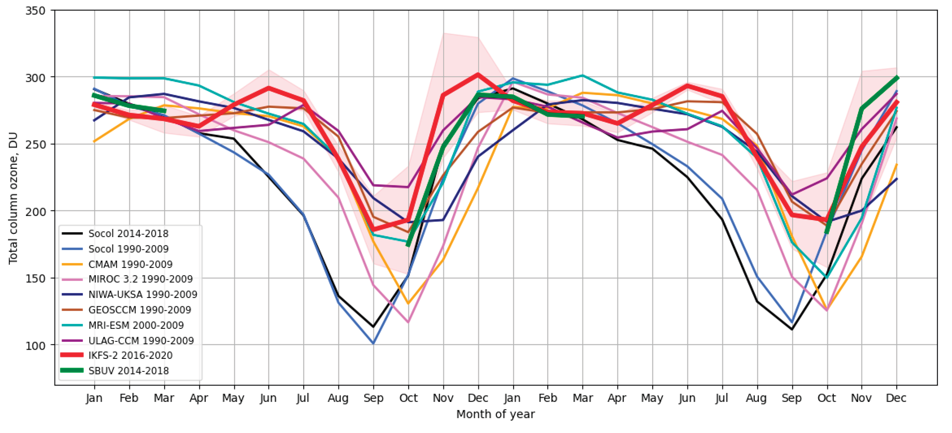
Figure 2.
The main components of the CCM SOCOLv3.
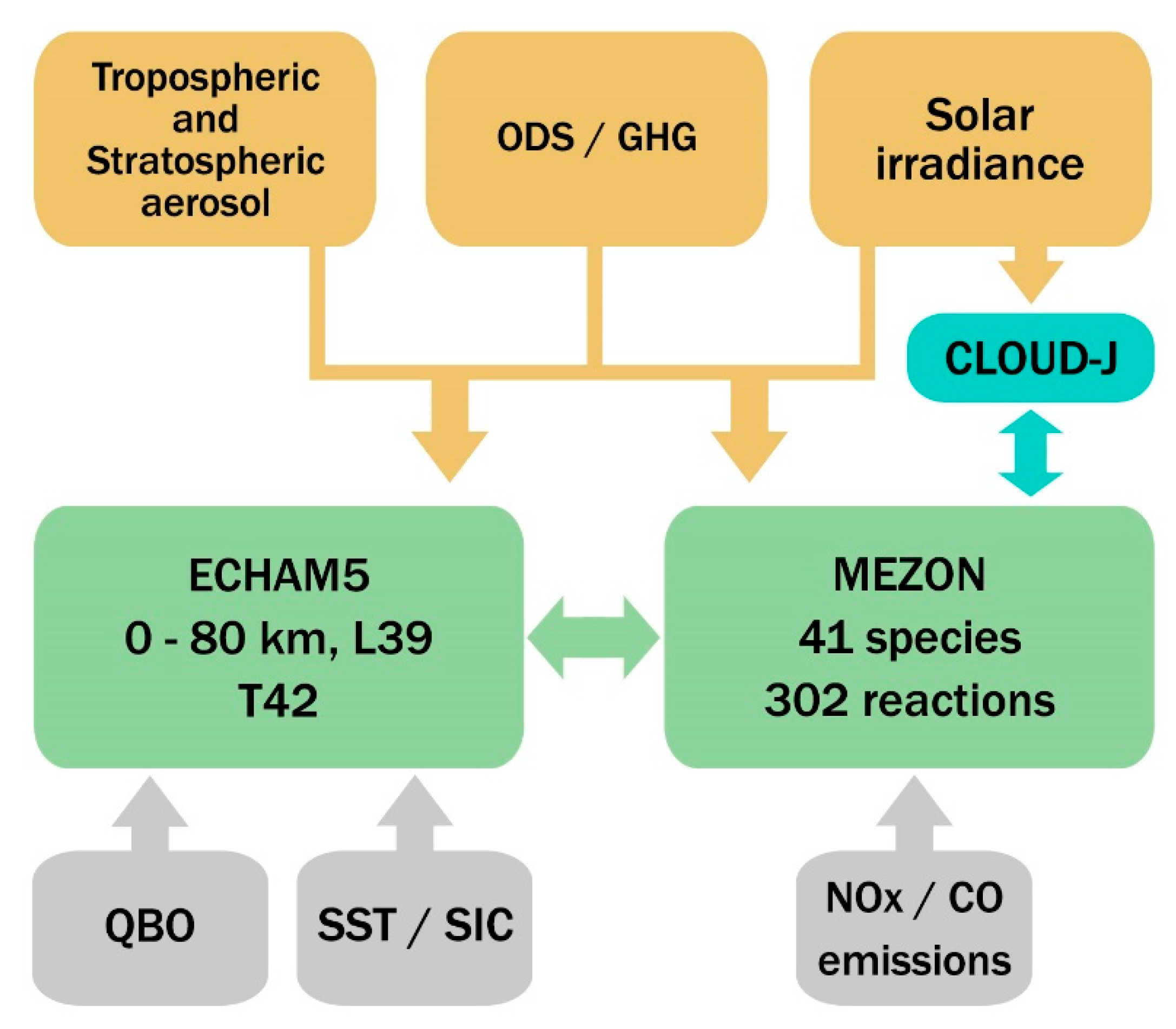
Figure 3.
TCO (DU) averaged over all Augusts during the 2016-2020 period from IKFS-2 data (a) and during the 2014-2018 period from the reference experiment (b).
Figure 3.
TCO (DU) averaged over all Augusts during the 2016-2020 period from IKFS-2 data (a) and during the 2014-2018 period from the reference experiment (b).
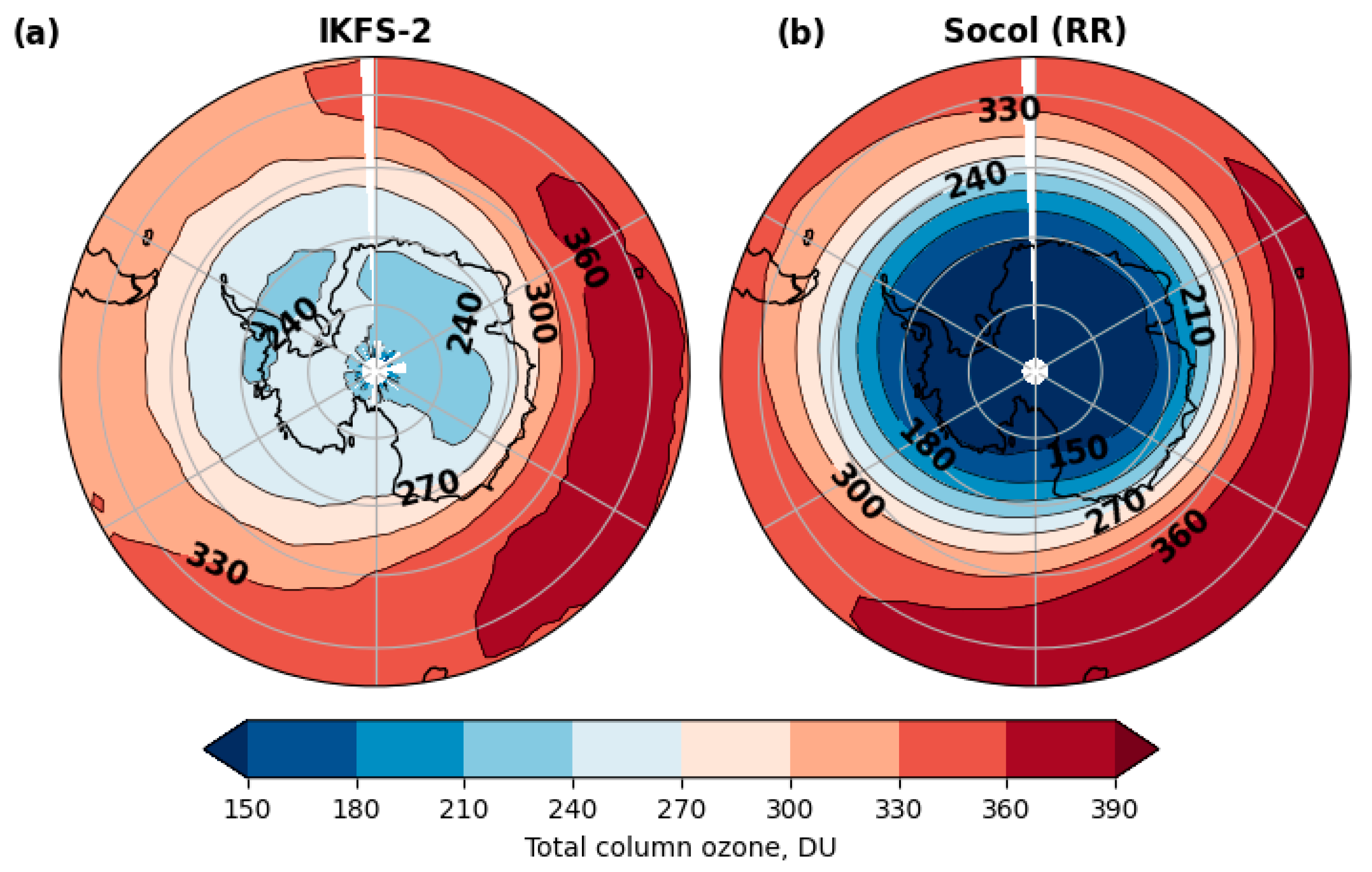
Figure 4.
Annual cycle of TCO (DU) at the 80S obtained from the IKFS-2 measurements (red) averaged over 2016-2020, and the reference(black), SR1 (orange), SR2 (blue), SR3 (cyan) experiments, averaged over 2014-2018.
Figure 4.
Annual cycle of TCO (DU) at the 80S obtained from the IKFS-2 measurements (red) averaged over 2016-2020, and the reference(black), SR1 (orange), SR2 (blue), SR3 (cyan) experiments, averaged over 2014-2018.
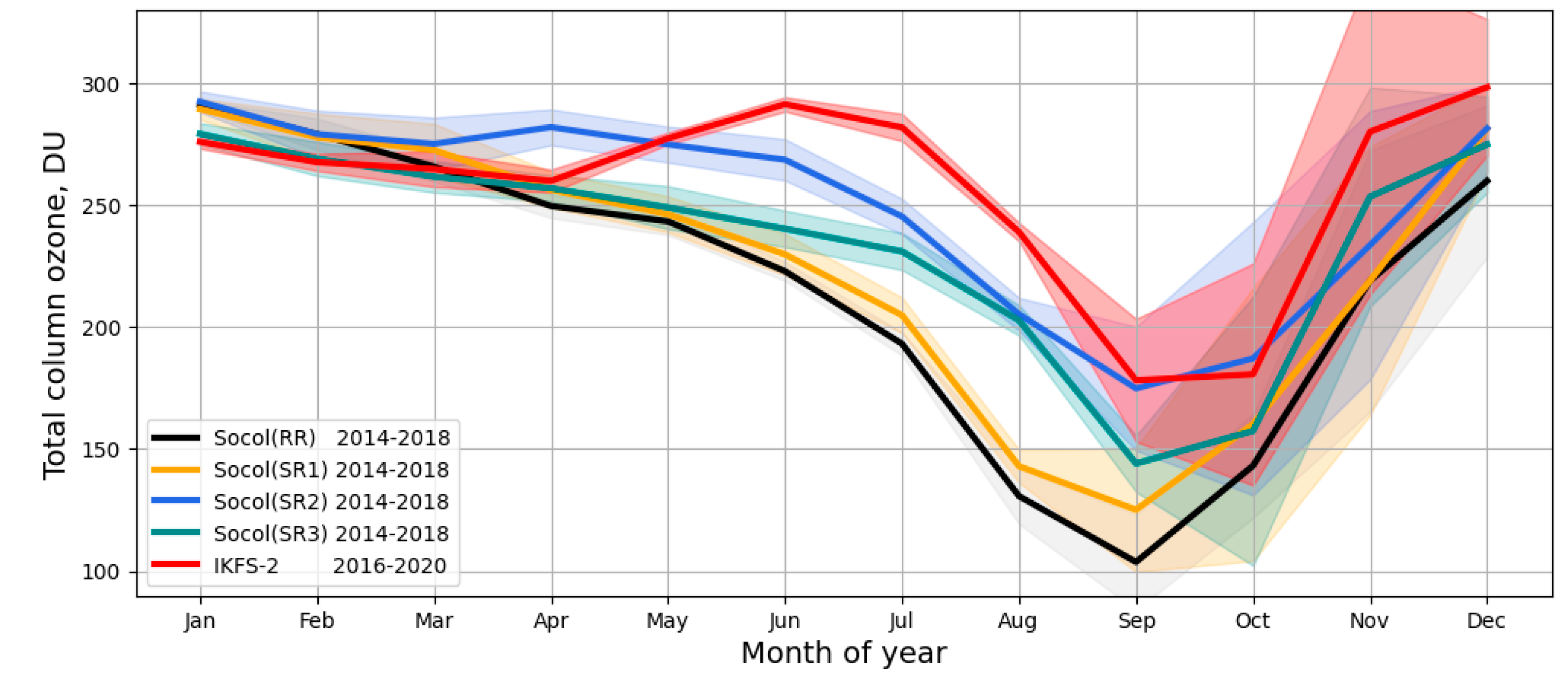
Figure 5.
The time-latitudinal mask of Kyy value with maximum equals 5·106 m2/s (SR2 experiment).
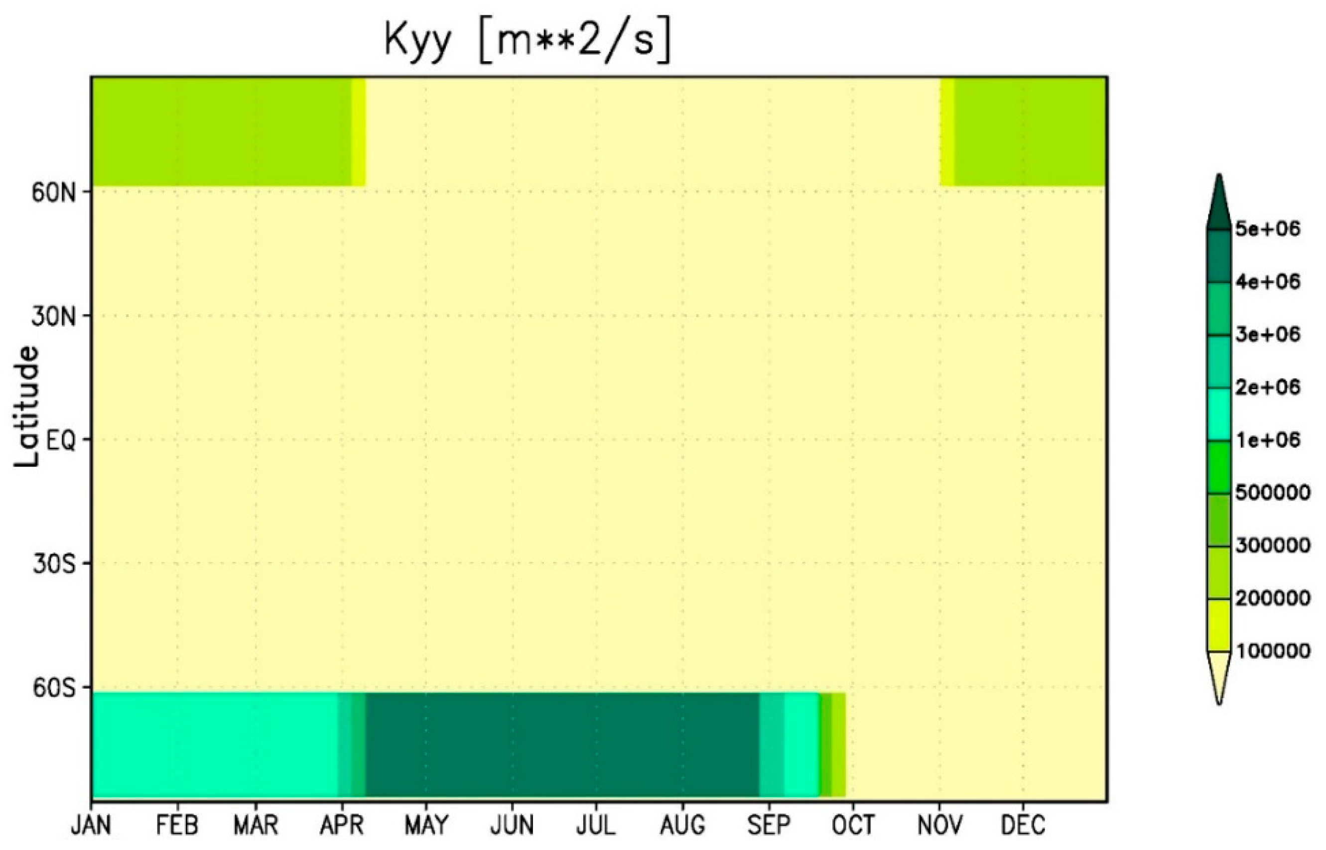
Figure 6.
Difference in O3 (ppmv) between reference simulation and MLS (a), N2O (ppmv) reference simulation and MLS (b), CH4 (ppmv) reference simulation and MIPAS data (c), O3 (ppmv) SR2 experiment and MLS (d), N2O (ppmv) SR2 experiment and MLS (e), CH4 (ppmv) SR2 experiment and MIPAS (f) in August for the Southern Hemisphere (45-80°S), averaged over 2014-2018. Statistically significant results are highlighted in color.
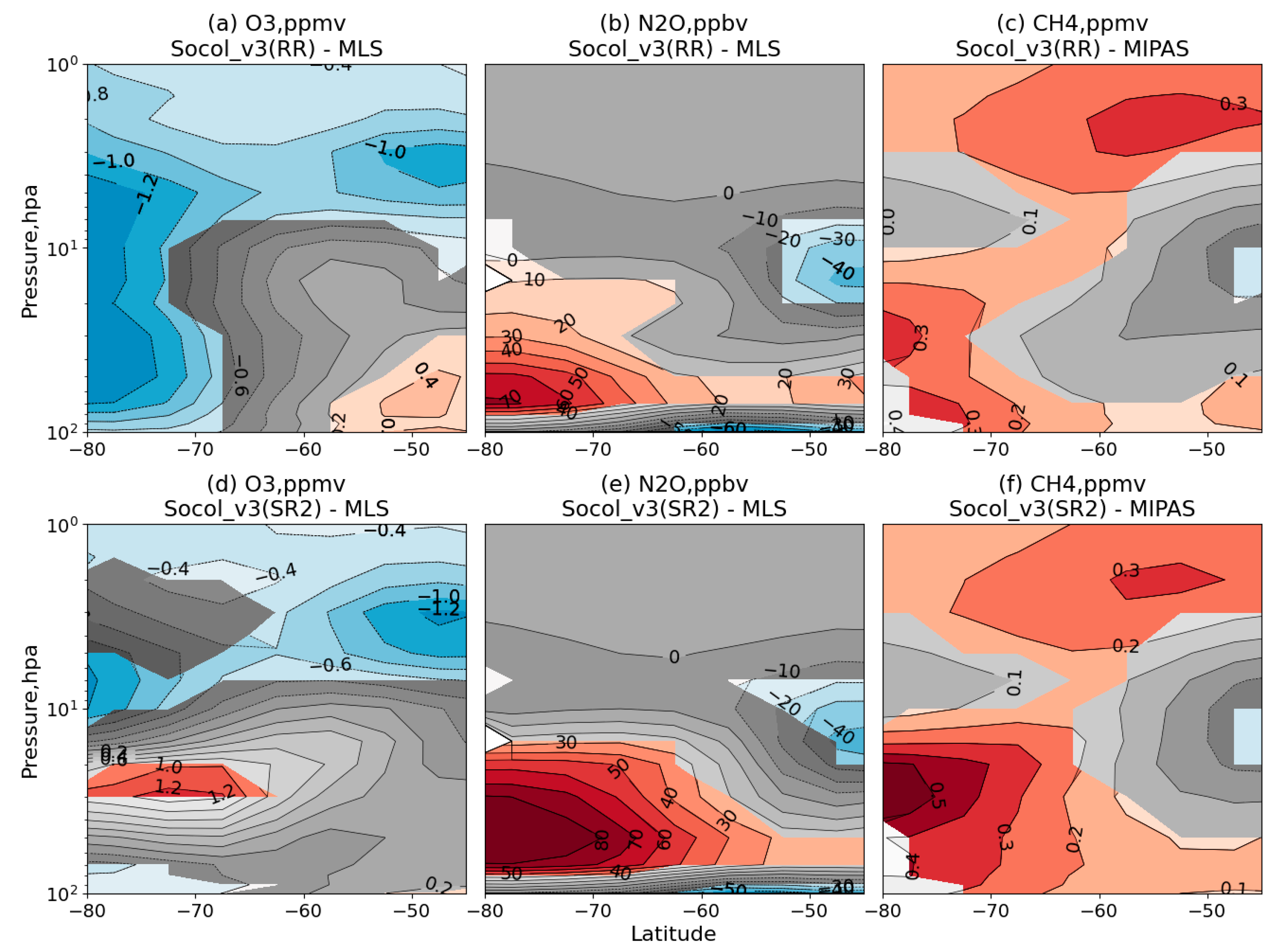
Figure 7.
Difference in TCO (DU) between reference run (a), SR3 run (b), and IKFS-2 data for months from June to September over the 2014-2018 period. Statistically significant results are highlighted in color.
Figure 7.
Difference in TCO (DU) between reference run (a), SR3 run (b), and IKFS-2 data for months from June to September over the 2014-2018 period. Statistically significant results are highlighted in color.
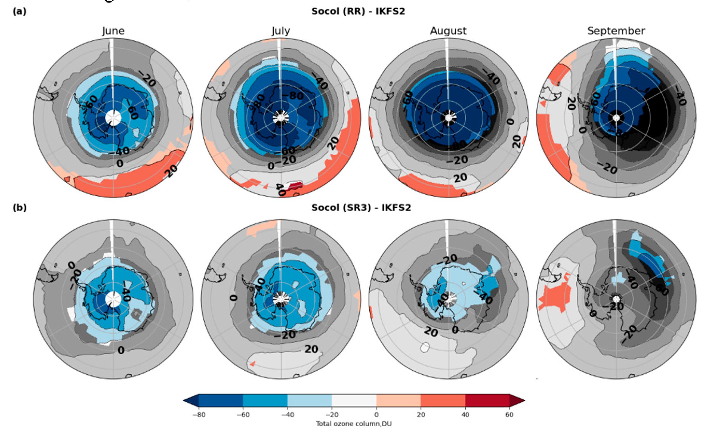
Figure 8.
O2 and O3 (total) photolysis rates inside the polar vortex at latitude 71°S on 1 August.
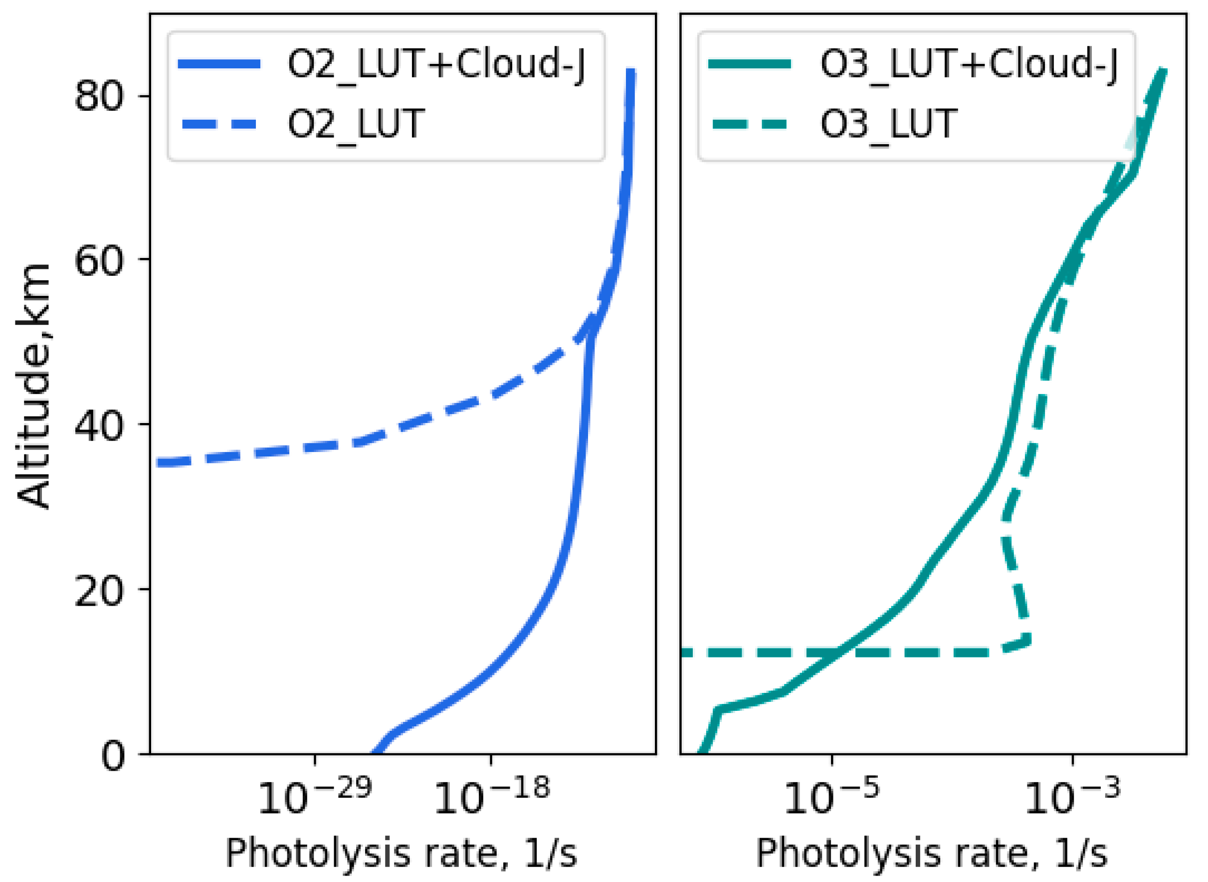
Figure 9.
The annual course of the absolute deviation (ppbv) between the reference experiment and the SR3 experiment for HCl and ClOx family (a) and the relative deviation (%) for O3, OH, O(1D) (b) at 70°S for the period 2016-2020.
Figure 9.
The annual course of the absolute deviation (ppbv) between the reference experiment and the SR3 experiment for HCl and ClOx family (a) and the relative deviation (%) for O3, OH, O(1D) (b) at 70°S for the period 2016-2020.
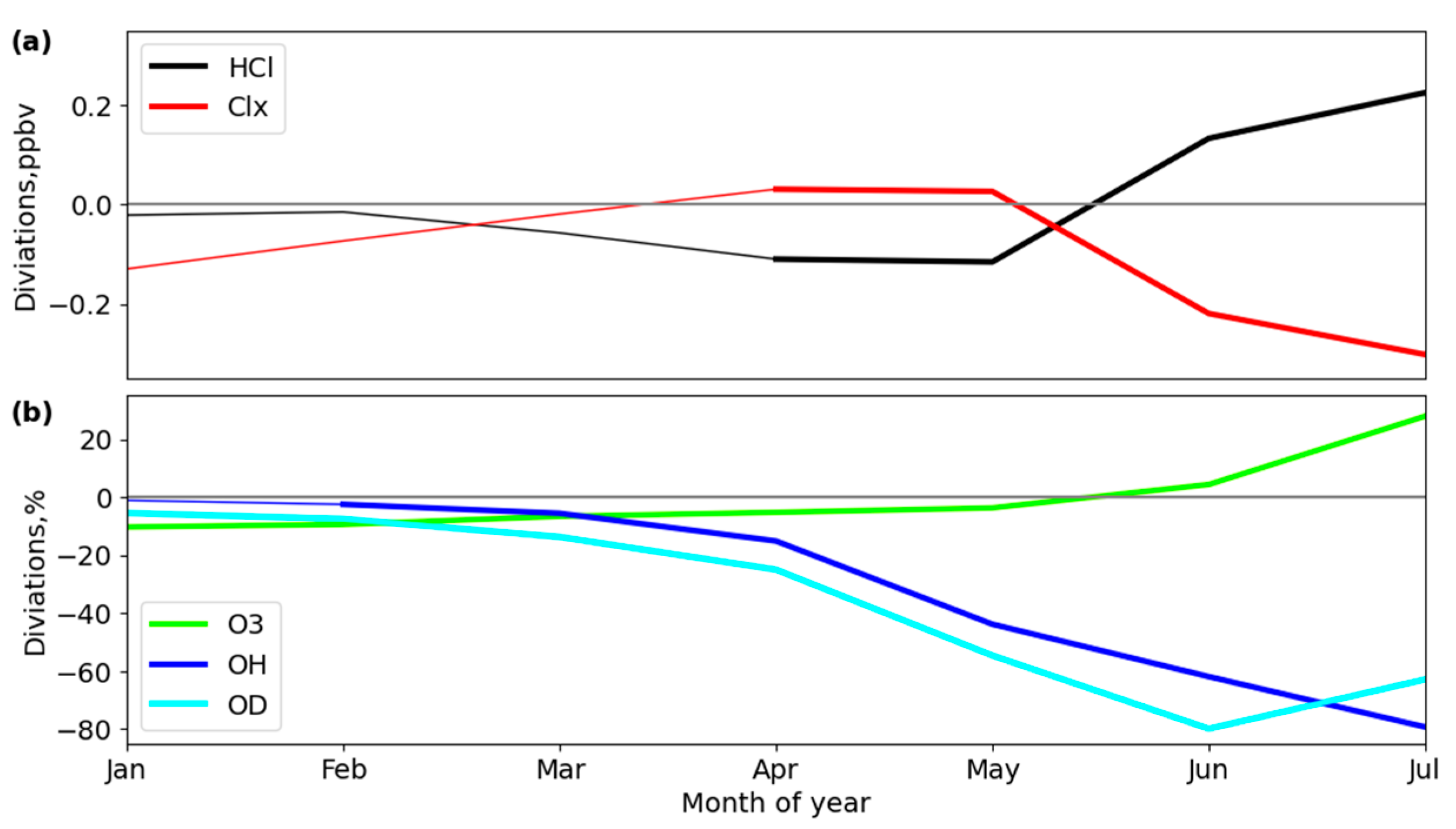
Figure 10.
Difference in zonal mean O3 (ppmv) between reference experiment (a), SR2 experiment (b), and MLS observations for the Southern Hemisphere (45-80°S) averaged over the 2014-218 period. Statistically significant results are highlighted in color.
Figure 10.
Difference in zonal mean O3 (ppmv) between reference experiment (a), SR2 experiment (b), and MLS observations for the Southern Hemisphere (45-80°S) averaged over the 2014-218 period. Statistically significant results are highlighted in color.
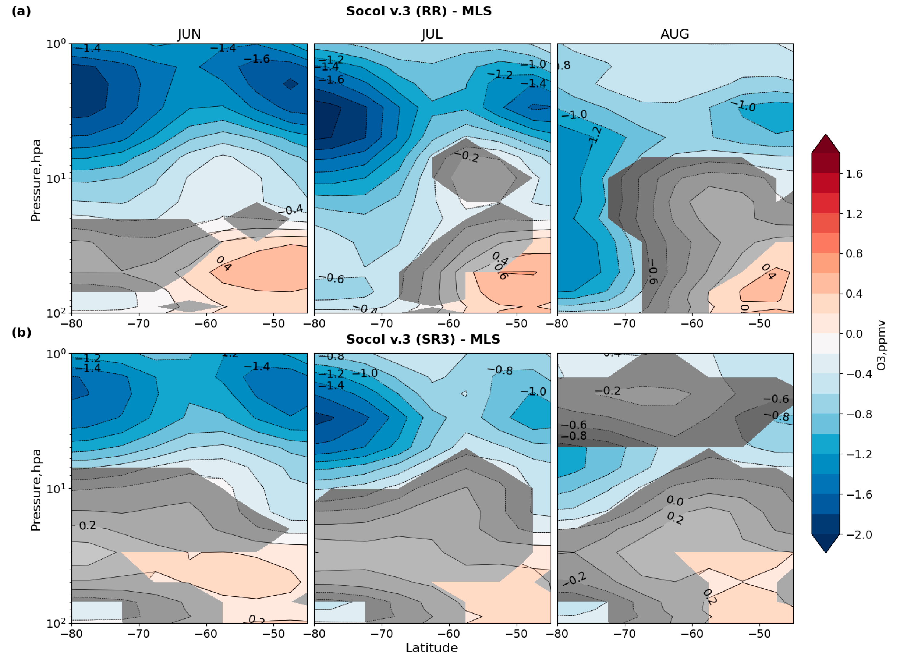
Figure 11.
Difference in N2O (ppbv) between reference experiment and MLS data (a), CH4 (ppmv) reference experiment and MIPAS data (b), N2O (ppbv) SR3 experiment and MLS data(c), CH4 (ppmv) SR3 experiment and MIPAS (d) in August for the Southern Hemisphere (45-80°S), averaged over 2016-2020. Statistically significant results are highlighted in color.
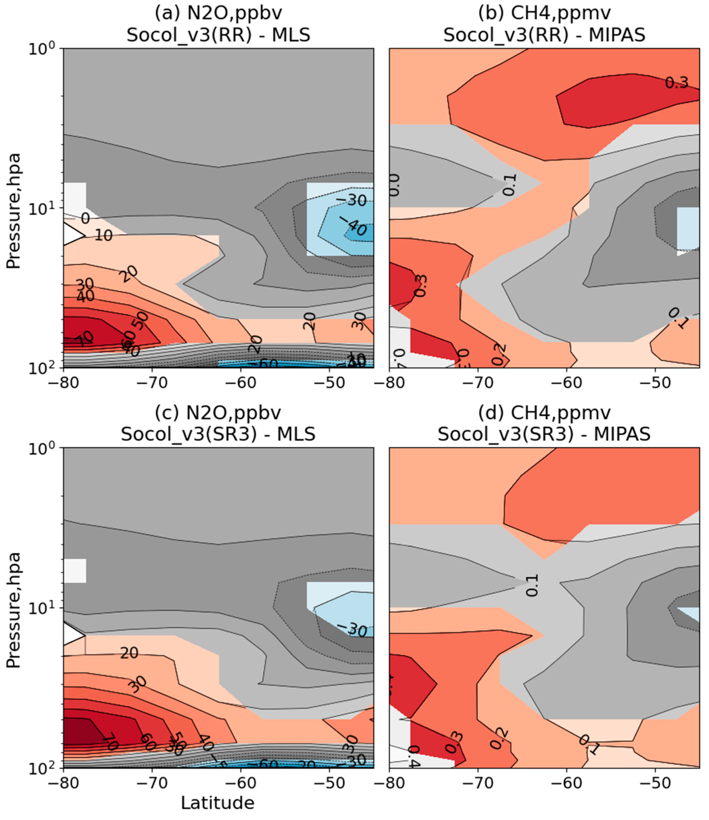

Table 1.
Description of the sensitivity experiments with CCM SOCOLv3.
| Name of model experiment | Short description of the model run |
| RR | Reference run described in 2.3.1 |
| SR1 | Two times reduction of the heterogeneous reaction HCl + ClONO2 → Cl2 + HNO3 rate. |
| SR2 | Intensification of the horizontal mixing process of all transported model species into the SH polar vortex with diffusion coefficient Kyy = 5·106 m2/s in its maximum. |
| SR3 | Using the Cloud-J v.8.0 module installed in the SOCOLv3 model to calculate photolysis rates |
Disclaimer/Publisher’s Note: The statements, opinions and data contained in all publications are solely those of the individual author(s) and contributor(s) and not of MDPI and/or the editor(s). MDPI and/or the editor(s) disclaim responsibility for any injury to people or property resulting from any ideas, methods, instructions or products referred to in the content. |
© 2025 by the authors. Licensee MDPI, Basel, Switzerland. This article is an open access article distributed under the terms and conditions of the Creative Commons Attribution (CC BY) license (http://creativecommons.org/licenses/by/4.0/).
Copyright: This open access article is published under a Creative Commons CC BY 4.0 license, which permit the free download, distribution, and reuse, provided that the author and preprint are cited in any reuse.


