
Submitted:
18 November 2023
Posted:
21 November 2023
You are already at the latest version
Abstract
The paper presents the observational, remote sensing and model simulation to analyze Southern Brazil Antarctic Ozone Hole influence (SBAOHI) events occurred between 2005 and 2014. To an-alyze it we use Total Ozone Column (TOC) data provide by Brewer Spectrophotometer (BS) and OMI (Ozone Monitoring Instrument) instrument satellite, besides the AURA/MLS (Microwave Limb Sounder) instrument satellite ozone profiles was utilized with DYBAL (Dynamical Barrier Localization) code in MIMOSA (Modélisation Isentrope du transport Mésoéchelle de l’Ozone Stratosphérique par Advection) model Potential Vorticity (PV) fields. TOC has 7.0 ± 2.9 DU re-ductions average in 62 events. October have more events (30.7%). Polar Tongue events are 19.3% of total, being in October more frequently observed (50% of cases), with medium intensity (58.2%) and in stratosphere medium levels (55.0%). Already Polar Filament events (80.7%) are more frequent in September (32.0%), medium intensity (42.0%) and in stratosphere medium lev-els (40.7%). ENSO index positive phase influenced 61.3% of events, having dominance in all in-tensity categories (minor 57.9%, medium 51.6%, major 58.3%), while the equilibrium dominate the QBO influence with 50% of total cases in positive phase and 50 % in negative phase.
Keywords:
antarctic
; ozone
; MIMOSA model
1. Introduction
Ozone transport in stratosphere is an essential factor to define the atmospheric trace constituents concentration in particular regions through the globe [1,2], including the higher polar ozone concentrations compared with more production in equatorial region. However, the global scale stratospheric Brewer Dobson circulation, transporting ozone from equatorial region to polar region [3,4]. This stratospheric circulation is still frequently studied [5,6].
Stratospheric components transport as water vapor, nitrous oxide and ozone are studied by using the PV analyzes [7]. Authors as [8,9] first discussed the stratospheric isentropic surfaces. This variable is important to air masses dynamic tracing definition, behaving like an material surface that have potential temperature conservation [10]. Using PV as horizontal coordinate [11], one can determining the Stratospheric Polar Vortex (SPV) edge as your maximum gradient region, capturing the insulation distribution effects within the SPV [12,13]. Furthermore, meridional PV gradients and long-lived trace atmospheric gas, reveal that isentropic horizontal exchanges between tropical and extra-tropical regions are controlled by stratospheric dynamic barriers [14,15].
The polar South Hemisphere spring time ozone reduction, called "Antarctic Ozone Hole (AOH)" [16,17,18], is caused by Polar Stratospheric Vortex formation [19,20] and heterogenic reactions that occurs on polar stratospheric clouds surface [21,22]. Ozone Hole began to draw attention to scientific community and many studies have been done through polar ozone observational data in South Hemisphere [23,24,25], the same way but with important differences compared to North Hemisphere [26,27,28].
Climate change may affect the stratospheric dynamic and thermodynamic processes, increasing in polar vortex strength, thereby increasing ozone depletion on Polar Regions [29]. This ozone may also be destroyed and/or produced, due to solar variations [30] or influenced by the stratosphere temperature, which is highly influenced by winter stability and effects on polar vortex [31]. Furthermore, there are recent indications of Ozone Hole area reductions through the last decade [32,33].
Middle latitudes near Polar Regions may have their ozone content directly influenced by passing your border through this regions, reducing ozone and increasing ultraviolet radiation levels [34,35,36,37]. Polar vortex can be perturbed by planetary wave activity increasing and this contributes to polar vortex ejection, through polar filaments that move to middle latitudes [38]. Rossby wave breaking cause PV filaments events [11,39], carrying South Pole air masses into middle latitudes, indirectly influencing the TOC on these regions [40]. The polar air source are largely dominated by stratosphere vortex excursions and filaments events [41].
Ref. [42] Presented stratospheric ozone extreme anomalies observed in middle latitudes related to stratospheric meridional transport over regions. Polar filaments may be isolated for 7 to 20 days after polar vortex separation, and this may be sufficient for their lower and middle latitudes propagation, causing a temporary TOC reduction [43,44,45]. The local ozone profiles measurement reveals particular anomalies or lamina when passing these filaments [46]. The global character of these stratospheric transport from polar region toward middle latitudes in South Hemisphere was registered on South America [35,47], South Africa [48] and New Zealand [49].
High resolution transport models [50,51] or contour advection [52] can correctly depict the ozone reduction lamina observed. Moreover, [53], using a PV contour advection MIMOSA model (Modele Isentropique du transport Mesoechelle de l’Ozone Stratospherique par Advection) [54] analyzed an important middle and tropical stratosphere isentropic exchange characterized by a PV lamina in 550 to 700 K isentropic levels, using the dynamical barrier locating code DYBAL (Dynamical Barrier Localization).
The cause of this transport, where occurs a deformation of PV contours over isentropic surfaces, are explained by planetary wave breaking [55]. The near-stationary mid-latitude winter planetary waves are known to propagate from the troposphere to stratosphere and meridionally toward the equatorial regions [56]. By E-P flux convergence, on can identify the breaking in Planetary wave and this can the cause of several stratospheric isentropic transport events [53,57,58,59].
Air masses originating in Ozone Hole passing over middle latitudes was first registered by [60], causing a TCO temporary reduction about 60 DU for that event. [61] Observed that a 1% TOC reduction In this planet part cause 1.2% ultraviolet radiation (UVR) average increase. Furthermore, the ultraviolet radiation the increase associated to ozone reduction can affect to the aquatic and terrestrial systems, being one factors that help to explaining the species decline related to malformations caused by UVR levels increase [62].
This decline in biodiversity serves to emphasize these objective study importance and the necessity to monitor ozone in these region. Furthermore, the observations made by BS for more than twenty years there show a good correlation with instruments satellite measurements, with annual cycle dominated the seasonal variability and interannual variability dominated by Quasi-Biennial Oscillation (QBO) and demonstrated by wavelet analysis and data series comparisons [63]. Climate model projections [64,65] demonstrated that increase in greenhouse gases concentration results in temperature and stratospheric circulation changes and affect global scale ozone content.
More recently, using SSO ozone observations [66,67] identified a significant TOC reduction for October,2016, due to AOH influence that reaching Uruguay and Brazil. Similarly, [68], between 1979 and 2013, also observed 62 events these type. As an initiative to predict this events occurrence, [69] calculated O3 indices that showed great dexterity in representing these events, indicating the polar trough that advanced on Southern Brazil with the largest negative O3 anomalies.
This paper analyses the TOC dataset taken using BS2 and OMI instrument satellite, complemented by AURA/MLS ozone profiles followed by MIMOSA model PV fields to report these polar and middle latitudes stratospheric isentropic exchange events from 2005 to 2014. This period covers 10 years of observations from Brewer (since 1992) and AURA/MLS (since the end 2004), and ozone data from those instruments are simulated by MIMOSA model to describe the events during this period.
First, the TOC reduction days were selected in BS and OMI time series. Next, the low vertical extension ozone lamina was investigated from the AURA/MLS satellite ozone profiles. Subsequently, a air masses origin diagnosis was conducted applying DYBAL code in PV fields by MIMOSA model to observed reductions levels in AURA/MLS ozone profiles to identify polar origin in these SBAOHI events and determine the dynamic barriers geographic locations. Finally, the statistics and classification of phenomenon occurrence and summaries, discussion and conclusions are provided in the least sections.
2. Materials and Methods
2.1. Ozone Experiments
Brewer Spectrophotometers are the fully automated ground based instruments developed for spectral irradiance measurements in the solar UVB range at five discrete wavelengths, namely 306.3, 310.1, 313.5, 316.8 and 320.1 nm, with approximately 0.5 nm resolution, allowing Nitrogen Dioxide (NO2) Sulfur Dioxide (SO2) and Ozone (O3) total column deduction. They can also obtain the atmospheric aerosols optical thickness and ozone profiles by Umkehr technique [70,71]. The BS TOC observations was done since 1992 through the instruments MKIV #081 (1992- 1999), MKII #056 (2000-2002), and since 2002 by MKIII #167 in Southern Space Observatory - SSO (29.26 ° S, 53.48 ° W), Brazil [72], belong to the Brazilian Brewer Network.
Ozone Monitoring Instrument (OMI) is an instrument aboard Aura satellite, operating since July 2004 in Earth Observing System (EOS) mission framework. OMI instrument do atmospheric components, as O3, NO2, SO2 and aerosols total column measures and the data can be downloaded from the NASA website: https://avdc.gsfc.nasa.gov/index.php. OMI performs measurements through the Backscatter Ultraviolet technique in a two images feeding the spectrometer grid. It has two UV bands, namely the UV-1 270 at 314 nm and the UV-2 306 at 380 nm with 1 – 0.45 nm spectral resolution [73].
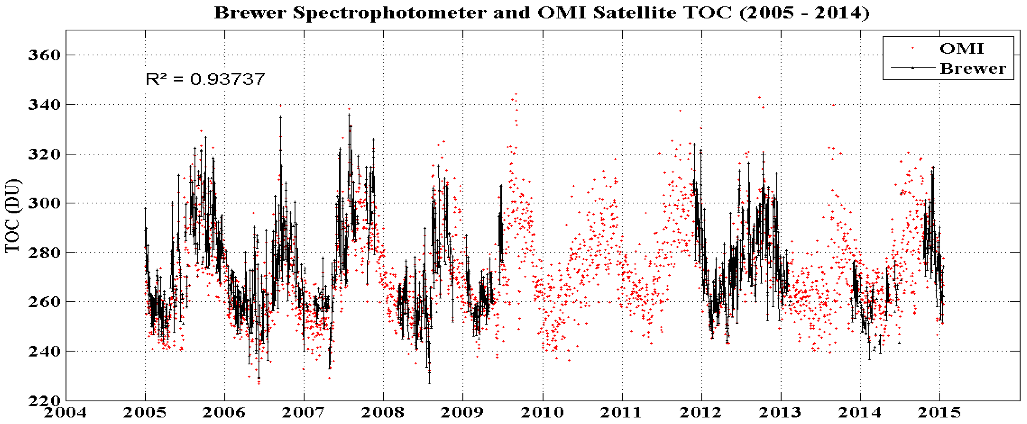
The BS #167 installed in the SSO and OMI instrument during 2005 to 2014 provides the TOC daily averages analyzed. For this same period, TOC daily averages from OMI instrument satellite are also obtained with the intention of performing a brief comparative analysis, and has a strong correlation between both measurements, presented in Figure 1, with R2 = 0.93. These results are in line with [63] to SSO station and other mid-latitude stations around globe, such as Lauder [49] and Iberian Peninsula [77], highlighting the confidence of both TOC data sets.
2.2. AURA/MLS Satellite Ozone Profiles Experiment
The AURA/MLS (Microwave Limb Sounder) is an instrument aboard Aura satellite, which participates in the EOS (Earth Observing System) program and launched in 2004 [78] and maintains a synchronous orbit with the Sun, near-polar, 700 km altitude and at an inclination of 98°. Basic information and v4.3 Aura / MLS O3 data is available through the link: http://mls.jpl.nasa.gov/products/o3_product.php. The MLS instrument is capable of providing global coverage between the latitudes of ± 82 ° for each day, running around 240 "scans" with each orbit with an extent of about 3500 profiles per day for 17 atmospheric parameters including ozone within 41pressure levels (218-0.01 hPa). MLS measures microwave thermal emission from the limb and records the vertical profiles of trace gases including ozone, BrO, ClO, CO, H2O, HCl, HCN, HNO3, N2O and SO2. Ozone is registered using the 240 GHz spectral region. The MLS vertical resolution ranges are 2.7 km to 3 km from upper troposphere to lower mesosphere. For each data acquisition errors in these measurements must be estimated, and with respect to ozone error is about ~5-10% range on stratosphere [79]. Initially, ozone profiles from AURA/MLS version v4.2 were selected in an area ranging from ± 5 ° latitude and longitude around the SSO region. From the four ozone profiles closest to the SSO location, daily profiles were calculated between 2005 and 2014. Subsequently these profiles were interpolated at 350 K to 950 K heights using the same vertical range utilized in PV fields by MIMOSA model.
2.3. Stratospheric Dynamic Diagnosis by DYBAL Code in MIMOSA Model PV Fields
The MIMOSA (Modélisation Isentrope du transport Mésoéchelle de l’Ozone Stratosphérique par Advection) model, is a three-dimensional high-resolution Potential Vorticity (PV) advection model. This model has been used to study the ozone lamina observed at Observatoire de Haute-Provence (OHP, 44°N, 5.7°E) by Lidar profiles and to plan the launch of an airborne ozone Lidar as [54,80,81]. The dynamical MIMOSA model is particularly used to describe filamentary structure through PV advection, since we can assume that the PV and ozone are very well correlated on an isentropic surface. Consequently, the location of ozone filaments can be determined using PV fields like a dynamical tracer [10,82].
The simulation started at 012 UTC on 01 May 2005 and ended at 012 UTC on 30 November 2014 including the spin-up period (~1 month) on an orthogonal grid in an azimuthal equidistant projection centered in South Pole (parallels are represented as concentric equidistant circles). The model runs on an isentropic surface and covers the whole southern hemisphere, extended between latitudes 10°N and 90°S for an horizontal resolution with elementary grid cell size of 37 X 37 km (three grid points/degree of latitude). Meteorological data was obtained at intervals of six hours by the European Center for Medium Range Weather Forecast (ECMWF) analysis at 1.125° latitude x longitude resolution and were provided by Third European Stratospheric Experiment on Ozone (THESEO) database set up at the Norwegian Institute for Air Research (NILU). Data were first interpolated at a vertical grid spacing that consisted of 25 isentropic vertical levels from 350 K to 950 K with a resolution of 2 km on the fine MIMOSA grid, and subsequently PV fields are extracted [40]. The numerical diffusion induced by the regridding processes are minimized by an interpolation scheme that uses the second order moments of PV [54].
The deformations caused by subtropical and polar vortex barriers are inferred from DYBAL code software using area coordinates and Nakamura’s formalism [83]. The Dybal code aims to localize the dynamic barrier zones in PV fields. The principle is to point out, in a PV field, the regions corresponding to the maximum ∂PV/∂A (PV gradient) and simultaneously the minimum Le2 (effective diffusivity), for the dynamic barriers locations. Together with a geographic location, DYBAL provides an indication of the strength of these barriers, measured from the secondary maximum PV gradient. This code allows emphasis to be given to the development of polar and subtropical filaments with high precision for their location, as presented in detail by [53]. Having a PV field for time t, first, ∂PV/∂λ and Le2 (λ) are calculated on basis of equivalent latitude on PV fields, then, the zones of Le2 (λ) minimum and maximum ∂PV/∂λ are digitally detected. A threshold of 1° of equivalent latitude around the maximum and minimum is applied. Throughout this study, PV fields are used at a 1 ° x 1 ° resolution and higher than 0.5 ° of equivalent latitude threshold. When both criteria are validated (maximum ∂PV/∂λ and L2 (λ) minimum), the equivalent latitude area is taken as dynamic barrier [57].
2.4. Methodology
The first criterion to identify SBAOHI events for 2005 to 2014 was to look for TOC reductions days measured by BS #167 and OMI instrument satellite. The criterion adopted should avoid 3% reductions of the monthly climatology, since these types of reductions in TOC can only be caused by tropospheric variations [84]. Considering this, TCO reductions were determined when the TOC daily average value was lower than -1.5σ limit. These dates with low TOC values were then selected for later verification if air masses came or not from polar region. The August to November climatological values with their standard deviations and -1.5σ limit for SSO station, obtained by [63] are show in Table 1.
Figure 1.
TOC datasets obtained by BS (black) and OMI instrument satellite (red) for the August-November period at SSO station.
Figure 1.
TOC datasets obtained by BS (black) and OMI instrument satellite (red) for the August-November period at SSO station.
We analyzed only the months between August and November, because this is the AOH activity period. This criterion means that if the data were placed over a normal frequency distribution, we would work with the extreme minimum values, representing 6.6% of total days [85]. These TOC reductions can no longer be totally credited to tropospheric variations, with photochemistry and transport in stratosphere being important to explain these reductions, thus supporting the choice of this period.
The statistical criterion -1.5σ limit was chosen after numerous tests, where it was determined that the mean limit minus 1 standard deviation (μ-1σ) or mean minus 2 standard deviations (μ-2σ) could not be used. First case, the differences around the average are near to 3%, and these values can be attained by changes in tropospheric ozone. If the last case, only a few days would be analyzed, and therefore, proven SBAOHI events would be missed and not analyzed.
From monthly ozone profiles time series, average, σ and -1,5σ limit from August to November were calculated. The second criterion was quantify the stratosphere laminar structures height that cause the TOC reductions observed by the BS and OMI instrument satellite. During days with ozone reductions during August to November that were selected in the previous section through the ozone percent differences profiles between the climatological profile and the reduction day profile, as in Equation 1. This shows the poor in ozone transport levels, demonstrating, with BS, the temporal and vertical ozone content distribution. This information is needed to make the stratospheric dynamic diagnosis that point these ozone reductions using MIMOSA model PV fields simulation and the dynamic barriers localization tool - DYBAL Code.
The third criterion is verify the stratospheric 350 to 950 K levels MIMOSA model PV fields. This procedure identify air masses origin that cause such TOC reduction measured by BS and OMI instrument satellite and ozone profiles by the AURA/MLS satellite.
These analyses verify if there was some variation in Absolute PV fields (APV) MIMOSA model between the reduction days and previous and posterior days. So making a vertical and temporal stratospheric dynamic diagnosis, since an PV increase is an polar origin indication and a decrease indicates that it comes from equatorial region [48,59]. The DYBAL code is used to check the exact location of subtropical and polar vortex filaments related to SSO station geographical position. If the air polar that cause this ozone depletion is verified, the day is a confirmed SBAOHI events.
To analyze these relationship between the events intensity and climatic indexes such as Quasi Biennial Oscillation (QBO) and El Niño / Southern Oscillation (ENSO), data were taking from the NOAA website: https://www.esrl.noaa.gov/psd/data/climateindices/list/.
3. Results
SBAOHI events between 2005 and 2014 were identified using the three mentioned criteria in the methodology. These criteria are TOC reductions in BS #167 and OMI instrument satellite time series, verification of the MLS ozone profiles reduction height and vertical and temporal stratospheric dynamic analysis by applying DYBAL code in MIMOSA model PV fields. This is made to check if air masses coming from polar region.
Figure 2 present the annual number of observation days by BS #167 (a) and OMI (b) (in blue), for the August-November period (in green) and number of days with below -1.5σ limit ozone reduction for each month (brown). Large gaps are evident in the Brewer observations between the period from mid-2009 to late 2011, and other shorter gaps between the end 2007 and beginning 2008 and after 2012. Some of these gaps are due some technical problems such as electronic breakdown, as described by [63].
This analysis resulted in 110 days with below -1.5σ limit ozone reduction over the SSO station, with an annual average of 11 days of reduction per year for the August-November period. However, in some cases, due to closeness of dates, some TOC reduction events may have been counted more than one time, and once this had been checked, we confirmed 72 separate events.
Figure 3 (a) shows the BS #167 (in gray) and OMI (in brown) TOC values between August and November 2012, highlighting TOC below -1.5σ limit (black star line) in blue, to identify TOC reduction dates. Figure 3 (b) shows the corresponding time evolution of PV values at 670K level (~24 km altitude) on SSO station. The PV values increases demonstrate the air polar over this site. The days with TOC reduction below -1.5σ limit with an PV values increase, as in around October 14, 2012 were selected to stratospheric vertical MLS ozone profiles more isentropic trajectories distributions by combining DYBAL contours in MIMOSA PV fields analyzes.
In 2012, 33 TOC reduction dates were registered below -1.5σ limit between August and November. Due the proximity of the dates, nine (9) possible events were selected, and these days were August 06 and 18, September 05, 14 and 22, October 14 and 22 and also November 10 and 23. However, only November 23 did not confirm the SBAOHI event occurrence in both vertical and temporal PV MIMOSA model diagnosis. Polar origin was verified in eight (8) events at 2012 and this was realized for all other years in the 2005-2014 period.
One important event was in October 14, 2012. This case study demonstrate the vertical and temporal stratospheric dynamics diagnosis and confirm the efficiency of this methodology to confirm this events occurrence.
3.1. Event Study Case
October 14, 2012 was the more significant SBAOHI events observed by BS #167 between 2005 and 2014 period. This event reached approximately 252.6 DU (Figure 3), representing 13.4% TOC reduction from October climatology (290.2 ± 8.79 DU), with an PV increase up to 670 K. This case study is an application of the methodology to identify these events.
Figure 4 (a) present the October 14, 2012 and October climatology ozone profile obtained by AURA/MLS satellite instrument, as a potential temperature function on SSO region. Daily TCO reductions are notable when compared to 550 and 700 K levels October climatology. Figure 4 (b) shows the percent differences anomalies between the October climatology ozone profile and daily ozone profiles between October 10 and 16, 2012. Anomaly profiles with reduction from October 10 are observed. This reaching values lower than -20% on October 14 to 550 and 700 K laminas and this reduction can still be observed, although it became less intense on subsequent days.
The DYBAL code applied to MIMOSA model PV fields are used to verify where the maximum PV gradient (∂PV/∂A) and minimum simultaneous effective diffusivity (Le2) are found. This procedure detect subtropical and polar dynamic barriers position [83,87]. The subtropical (red line) and polar (black line) barriers positioning, calculated by the DYBAL code, and the SSO region (black X) are presented through vertical (Figure 5) and temporal (Figure 6) stratospheric dynamics diagnosis in MIMOSA PV fields.
This analysis are performed to identify what air masses origin that arriving in SSO station on the selected reduction days where ozone depletion lamina in the AURA/MLS satellite profiles were found. The vertical DYBAL outputs distribution in MIMOSA PV fields for 400, 450, 500, 525, 675 and 850 K levels for the October 14, 2012 event are presented on Figure 5. That objective to verify which stratospheric vertical structure during events occurrence. To classify whether these are polar filaments or polar tongues in MIMOSA PV fields, it was assumed that a polar filament occurs when only PV filaments are observed, but polar tongue occurs when a large PV filament surrounded by polar barrier line on SSO region was observed.
On SSO region, 400 K level shows the subtropical barrier. From 450 to 525 K levels, polar origin is observed due the higher PV values presence as a polar filament. From 675 to 850 K levels, a very intense polar tongue with a higher PV value with polar barrier. These results give indications of an intense transport from polar region toward the sub tropic.
Figure 5 present that above 500 K level the high PV values polar tongue positioning, in the study area, is more evident in 675 K. This corroborates with largest AURA/MLS ozone profile negative anomaly observed as in Figure 4. Additionally, a temporal analysis at this isentropic level (675K) using the DYBAL outputs (dynamical barrier locations) superimposed with the corresponding MIMOSA model PV fields before and after “14 October event” was performed.
Figure 6 show an intense higher PV Polar Tongue presence surrounded by polar barrier line over Central and Southern Argentina on October 08. This Polar Tongue moves northward and reaches the SSO station on October 14, moving further north and losing intensity on October 16 on Atlantic Ocean causing the observed reductions in BS #167 and OMI TOC and in AURA / MLS satellite ozone profile to this period.
These results are explained for studies on polar filamentation effects in mid latitude stratosphere caused by transport between pole and mid latitudes mixing zone conducted by [54,88]. In addition, our results are consistent with previously reported disturbances caused by AOH influence events on 30 °S [60] and polar filaments over mid latitude sites reported by [41]. This analysis shows that the intense polar tongue of high PV values surrounded by polar barrier was ejected in direction to Southern Brazil, confirming the event occurrence in October 14, 2012.
3.2. Statistics and Classification of SBAOHI events between 2005 and 2014
When applying the same methodology used in 2012 for 2005 to 2014 period, the TOC reductions day resulted in 110 days below -1.5σ limit, with an annual average of 11 days of TOC reduction per year. However, in function of proximity dates, TOC reductions can by caused for the same polar transport. 72 possible events were separated, wherein 62 were confirmed by the vertical and temporal stratospheric dynamics diagnosis.
This analysis is performed by detecting the AURA/MLS satellite ozone profiles lamina reduction height and the transport from the AOH to SSO station, and through dynamic barriers position verification from DYBAL code applied in MIMOSA model PV fields. Less than 15% (13.8%) ozone reduction events were not confirmed as being due SBAOHI events.
A summary of the 62 confirmed SBAOHI events between 2005 and 2014 is presented on Table S1 in the supplementary material. This synthesizes the event occurrence dates, the TOC values, percent reduction respective to monthly climatology, the isentropic level of the AURA/MLS satellite ozone profile reduction, and their maximum percent reduction.
Additionally, the characteristics and levels of polar transport to the SSO station region through the application of the DYBAL code in MIMOSA model PV fields are presented. Thus, polar filaments (PV filament only) or polar languages (PV filament plus Polar barrier DYBAL line) in PV fields are detected in all events occurred on 2005 to 2014 period.
SBAOHI events occurs on average 6.2 ± 2.6 per year, with mean TOC reductions registered by BS #167 of 7.0 ± 2.9% and 7.7 ± 2.4% for OMI satellite. Furthermore, the mean isentropic level (K) and maximum mean AURA/MLS ozone profiles reduction occurred in 640 ± 150 K and 15.3 ± 6.3%, respectively. In October there are more events, 19 in total (30.7%), followed by September with 18 (29.1%), August with 14 (22.5%) and November with 11 (17.7%). Overall, only 19.3% of events showed polar tongue structures, while 80.7% of events presented polar filament structures.
In 400 K occurs only 4.89% of total events, while 10.48% at 450 K, 14.68% at 500 K, 18.88% at 600 K, 27.97% at 675 K, and 23.07% at 850 K. This kind of isentropic analysis allows the seasonal and geographical variability of the filament preferred forms of exchange identification [86] through nitrous oxide (N2O) laminar structures from a stratospheric three-dimensional chemical transport model, where during the winter and boreal spring, these structures are introduced from middle latitudes to the tropics. Using our analysis, we emphasize the 500 to 850K as the preferential levels of stratospheric transport with observed ozone depletion lamina when there are SBAOHI events.
This events occurrence is separate per year and month and illustrated in Figure 7. With 10 events, 2006 stands out as the year of greatest events occurrence, being 03 in August, 02 in September, 03 in October and 02 in November. This are explained because 2006 recorded the largest AOH area in the history (https://www.nasa.gov/vision/earth/lookingatearth/ozone_record.html).
Events was classified into three categories by taking into account (1) TOC reduction from BS #167 and OMI records intensity, (2) reduction lamina height determined from the corresponding AURA/MLS ozone profile and (3) the event dynamical shape form of a filament or tongue structure was identified from DYBAL code and MIMOSA PV maps.
Three intensity levels have been defined according to TOC reduction percentage (%TOC): Minor when %TOC is less than 6% (%TOC < 6%), Medium when %TOC is between 6 and 9% (6% ≤ %TOC < 9%), and Major when %TOC is greater than or equal to 9% (%TOC ≥ 9%).
The isentropic heights of occurrence events were divided in three layers: Low Stratosphere (LS) for X< 500 K; Medium Stratosphere (MS) for 500 K ≤ X <700 K and Upper Stratosphere (US) when X ≥ 700 K. It should be noted that an event can be identified in more than one height category.
Figure 8 shows plots of monthly ozone reduction events percentage events occurrences. The upper plots, (a) and (b), illustrate events statistics with a “tongue” structure, while the lower plots, (c) and (d), show distributions of events characterized by a “filament” structure. Moreover, plots on the left side of Figure 8 show the events distribution according to their intensity (Minor, Medium or Major); the plots on the right side indicate how the events are distributed in the tree stratospheric layers (LS, MS and US).
Polar Tongue characteristic were observed only in 19.3% (12 events). 01 in August (8.4% of cases), 02 in September (16.6 % of cases), 06 in October (50% of cases) and 03 in November (25% of cases), with medium intensity (58.2% of cases) and in stratosphere medium levels (55.0% of cases). Polar Filament characteristics were observed 80.7% of total cases and are distributed in 26.0% of cases in August, 32.0% September, 26.0% October and 16.0% November, with medium intensity (42.0% of cases) and in the medium level in stratosphere (40.7% of cases).
These results are consistent with [54,80] who used the MIMOSA model to identify the polar air presence in medium latitudes lower stratosphere (about 450 K). The simulations results allowed for interpretation of the laminar structures observed in vertical ozone profiles measured by the Light Detection and Ranging LIDAR of the Observatory of Haute Provence (OHP).
Climatic indexes that were found to have more influence on the events intensity appear to be Quasi Biennial Oscillation (QBO) and El Niño/Southern Oscillation (ENSO). This is due to these indices have cycles shorter than 10-year period analyzed here.
Figure 9 present the events occurrence intensity analyses. The QBO index (top) and the ENSO index (bottom) comparison to TOC reduction intensity where three classifications of intensity (i.e., minor events, medium events and major events) are presented separately by different colors.
The results show that the minor events (19 of 62) occurred more during the negative QBO phase and during the positive ENSO phase (57.9% in both cases), while the medium events (31 of 62) occurred more during the positive QBO phase (51.6%) and during the positive ENSO phase (64.5%). The major events (12 of 62) occurred mostly during the positive QBO phase and during the positive ENSO phase (58.3% in both cases). That can by influenced by the positive phase of ENSO index with 61.3% of total cases dominating the three categories of intensity, while the QBO index has 50% of total cases in positive and negative phases.
4. Discussions
TOC from OMI have good correlation with other TOC measurements observations in southern subtropics by Dobson and SAOZ spectrometers and ozone profiles [74,75], besides IASI European satellite instruments [76]. [63] Present a detailed description of TOC monitoring using BS in SSO for more than twenty years (1992 - 2014) and a comparison with satellites measurements. Thus, these instruments contribute scientifically by determining the seasonal variability dominated by the annual cycle, with minimum (~ 260 DU) in April and maximum (~ 295 DU) in September. Interannual variability is dominated by Quasi Biennial Oscillation (QBO) mode, identified by wavelets analysis and comparing the QBO index with the monthly TOC anomaly time series, and a condition of a near antiphase was described by these instruments.
Additionally, [89] demonstrated that deformation on a planetary scale led to the intrusion of tropical air tongues towards mid latitudes and numerically simulated the large-scale isentropic transport that increased the ozone over Réunion Island (55°E, 21°S) [53]. This result was due the med latitudes in the tropical stratosphere air masses displacement onto the ozone lamina, and DYBAL code was to identify the dynamic barriers positioning in the MIMOSA model.
Stratospheric ozone variability can be analyzed on a daily, seasonal, or annual basis, and can even be analyzed over a years period. The daily or weekly ozone variability are related to atmospheric systems, since high and low ozone values correspond to atmospheric systems, as occurring an inverse ozone and pressure correlation (low pressure corresponds to high ozone and vice-versa) [4]. The solar cycle shows that the sun activity occurs at approximately 11-year intervals, and ozone trends and stratosphere temperatures are largely due to ultraviolet solar flux variability associated with 11-year solar cycle [90].
One of climate change natural causes is the solar irradiation variability that occurs in a cycle of 11 years. Although the total changes in irradiance associated with solar cycle are insignificant (0.1%), much larger variations (4-8%) are found in UV range (200-250 nm) [91], a range that is crucial for the ozone photochemistry.
Based on a statistical study [92,93] suggested that during eastern QBO phase, the SPV is weaker and warmer (and vice versa for the western phase of QBO). In other words, these studies indicate that the eastern phase will lead to more intense wave activity and more frequent heating. These above mentioned studies suggested a mechanism by which the QBO phase can modulate the efficiency of the waveguide in mid-latitudes, which may facilitate the planetary waves propagation to Polar Regions.
In fact, planetary waves propagate from the extratropical troposphere through a wave guide of western winds. During the eastern phase of the QBO, the zonal Wind Slug slowly moves toward the winter hemisphere subtropical regions. As a result, the width of the western waveguide narrows leading to the planetary waves refraction away from subtropical latitudes towards the poles.
The results show that the high tropical stratosphere influences polar temperatures and winter stratospheric circulation [94,95]. For the large planetary wave structure across the entire stratosphere thickness, it seems quite likely that only QBO in lower equatorial stratosphere favors more pronounced planetary waves propagation to the poles [92].
Historically, EN events occur every 3-7 years and alternate with the opposite phase, which causes below-average temperatures in Tropical Pacific (LN). ENSO has global impacts, manifesting greater strength in the winter months in both hemispheres. Anomalies of sea level pressure are much larger in the temperate zones, while in the tropics there are larger variations in precipitation [96,97,98].
Like many other geophysical phenomena, ENSO is not stationary. Its temporal structure, however, is not as well documented as its spatial structure due the limited time of observations and the lack of adequate methodologies (non-linear analyses). In addition, [99] showed the interannual variability dominant mode on a planetary scale of ozone concentration been strongly associated with the El Niño Southern Oscillation (ENSO) phenomenon.
In addition, they noted that ozone concentration shows a strong connection with the ENSO wave 1 pattern in the temperate zones of Southern Hemisphere. The ENSO influence can be demonstrate since the positive phase of the ENSO index increases the polar vortex instability due to temperature increase. This more easily ejecting air masses from SPV to middle latitude regions, as observed by [13] with respect to 2002 AOH on the middle latitude regions impacts.
5. Conclusions
This paper presents the SBAOHI events occurrence between 2005 and 2014 observed by the BS #167, OMI and AURA / MLS satellites, and simulated by applying the DYBAL code in MIMOSA model PV fields. This was done to verify temporal and vertical distribution and intensity of TOC reductions. Atmospheric dynamic characteristics, and the climatic indexes such as QBO and ENSO influence during this phenomenon occurrence was identified.
The BS #167 and OMI satellite TOC on SSO station was compared in 2005 to 2014 period and good correlation (R2 = 0.93) is obtained between instruments. Thus validated TOC from both instruments are used for first stage to identify the SBAOHI events occurrence. In total, 110 ozone reduction days were selected in the August to November period, with an 11 days per year average. However, due the proximity of the dates, 72 possible events were selected for air mass origin analysis.
The October 14, 2012 event was taken as an example of applied this methodology to identify the events. This is the more significant BS event in the period 2005-2014 since it presented 252.6 DU TOC value, been this a 13.4% reduction comparing to October average (290.2 ± 8.79 DU). The AURA / MLS satellite ozone profile obtained on October 14, 2012 for the SSO region showed a substantial ozone reduction (~20%) in relation to October ozone profile for 550 at 700 K levels.
In addition, vertical and temporal stratosphere dynamics diagnosis provided by application of DYBAL code in MIMOSA model PV fields, showed an intense polar tongue of high PV values in the isentropic surfaces of 670 and 850 K passing on the SSO station region.
Applying the same methodology, 62 SBAOHI events were confirmed. This events occurred on 6.2 ± 2.6 times per year average, with mean TOC reductions by BS #167 of 7.0 ± 2.9% and OMI satellite of 7.7 ± 2.4%. In the AURA/MLS satellite, the mean isentropic level and maximum mean ozone profiles reduction occurred in 640 ± 150 K and 15.3 ± 6.3% respectively, assuring this kind of phenomenon importance when ozone reduction occurs in SSO region. Between 500 and 850K levels this events were identified applying Dybal code in MIMOSA model PV fields.
October is the month when have more events, 19 in total (30.7%), followed by September with 18 (29.1%), and 19.3% showed the Polar Tongue atmospheric characteristic while 80.7% presented the Polar Filament atmospheric characteristic. The 500 and 850 K levels were shown as the preferential levels of stratospheric transport when SBAOHI events. The year 2006 It was the year with the most events in a single year (10), while 2011 showed less events in a single year (01), and from 2012 to 2014 08 events occurred per year.
The events were separated into three categories: TOC reduction intensity, height of reduction lamina in ozone profile, and Filaments or Tongues as atmospheric dynamic characteristics. Only 19.3% of total cases were Polar Tongue, and these were more frequent in October (50%), with medium intensity (58.2%) and in stratosphere medium level (55.0%) in majority of cases. Polar Filament events (80.7%) were more frequent in September (32.0%), with medium intensity (42.0%) and in stratosphere medium level (40.7%) in majority of cases.
The SBAOHI events occurrence in the 2005 to 2014 period can be influenced by positive phase of ENSO index (with 61.3% of total cases), dominating the three categories of intensity (minor 57.9%, medium 51.6%, major 58.3%). Positive phase of the ENSO index increases the instability of the SPV due the temperature increase, more easily ejecting polar air masses into middle latitudes regions, while the QBO index does not have a clear influence since 50% of total cases were in positive and negative phases.
Author Contributions
Conceptualization, L.P., D.P., H.B, J.B., V.A. and N.B.; methodology, L.P., D.P., H.B, N.M, G.B., T.N., A.T., A.P. and R.T.; software and hardware, L.P, L.S, R.T., M.R. G.B., A.T. and N.M.; formal analysis, L.P.; data curation, L.P., G.B., D.P., J.B and M.M.; writing—Original draft preparation, L.P..; writing—Review & editing, L.P., G.R., G.B, J.V., R.S., D.P., H.B., N.M., A.T., M.M., L.A., N.B., T.N. V.A. and A.P.; funding acquisition, L.P., D.P., H.B., R.S., and M.M All authors have read and agreed to the published version of the manuscript.
Funding
CAPES (Coordination for the Improvement of Higher Education Personnel) a foundation linked to the Brazilian Ministry of Education, CAPES project number 88887.130199/2017—01 and COFECUB (French Evaluation Committee of the University and Scientific Cooperation with Brazil). Additionally to FAPESPA (Amazon Foundation for the Support of Studies and Re-search) and CNPQ (National Council for Scientific and Technological Development) an entity linked to the Ministry of Science, Technology and Innovations to encourage research in Brazil.
Data Availability Statement
Data available on request from L.P.
Acknowledgments
The MESO Project from CAPES/COFECUB Program (Process No. 88887.130176/2017-01). At Federal University of Western Pará (UFOPA), Graduate Program in Meteorology of the Federal University of Santa Maria (UFSM), with the Laboratory of Atmosphere and Cyclones (LACy) on University of Reunion Island (France), supported by Coordination for the Improvement of Higher Education Personnel (CAPES) Process no. 99999.010629/2014-09. The authors also the NASA/TOMS/OMI and NOAA climate index for the data used in the analysis.
Conflicts of Interest
The authors declare not conflict of interest.
References
- Gettelman, A., Hoor, P.; Pan, L. L., Randel, W. J., Hegglin, M. I., Birner, T. (2011), The Extratropical Upper Troposphere and Lower Stratosphere. Rev. Geophys., v. 49, n. RG3003. [CrossRef]
- Bracci, A., Cristofanelli, P., Sprenger, M., Bonafe, U., Calzolari, F., Duchi, R., Laj, P., Marinoni, A., Roccato, F., Vuillermoz, E., Bonasoni, P. (2012), Transport of Stratospheric Air Masses to the Nepal Climate Observatory-Pyramid (Himalaya; 5079 m MSL): A Synoptic-Scale Investigation. J Appl. Meteorol. Clim., v. 51, n. 8, p. 1489-1507. [CrossRef]
- Brewer, A. W. (1949), Evidence for a world circulation provided by the measurements of helium and water vapour distribution in the stratosphere, Q. J. R. Meteorol. Soc., v.75, p. 351-363. [CrossRef]
- Dobson, G. M. B. (1968), Forty years' research on atmospheric ozone at Oxford: A history. Appl. Opt., v. 7, p. 387-405. [CrossRef]
- Roscoe, H. K. (2006), The Brewer–Dobson circulation in the stratosphere and mesosphere – Is there a trend? J. Geophys. Res-Atmos., v. 38, p. 2446–2451. [CrossRef]
- Weber, M., Dikty, S., Burrows, J. P., Garny, H., Dameris, M., Kubin, A. J., Abalichin, J., Langematz, U. (2011), The Brewer-Dobson circulation and total ozone from seasonal to decadal time scales. Atmos. Chem. Phys., v. 11, p. 11221–11235. [CrossRef]
- Schoeberl, M. R. (1989), Reconstruction of the constituent distribution and trends in the Antarctic polar vortex from ER-2 flight observations, J. Geophys. Res., v.94, p.16.815– 16.845. [CrossRef]
- Danielsen, E. F. (1968), Stratospheric-tropospheric exchange based upon radioactivity, ozone and potential vorticity. J. Atmos. Sci., v. 25, p. 502-518. [CrossRef]
- Larry, D., Chipperfild, M., Pyle, J., Norton, W., Riishojgaard. L. (1995), Tree-dimensional tracer initialization and general diagnostics using equivalent PV latitude-potential-temperature coordinates, Q. J. Roy. Metror. Soc., v. 121, p. 187– 210. [CrossRef]
- Hoskins, B. J., McIntyre, M. E., Robertson, A. W. (1985), On the use and significance of isentropic potential vorticity maps. Q. J. Roy. Metror. Soc., v. 111, p. 877-946. [CrossRef]
- Norton, W. A. (1994), Breaking Rossby waves in a model stratosphere diagnosed by a vortex – following coordinate system and a technique for advecting material contours. J. Atmos. Sci., v. 51, p. 654-673. [CrossRef]
- Nash, E. R., Newman, P. A., Rosenfield, J. E., Schoeberl, M. E. (1996), An objective determination of the polar vortex using Ertel’s potential vorticity. J. Geophys. Res., v. 101, p. 9471–9478. [CrossRef]
- Marchand, M., Bekki, S., Pazmiño, A., Lefèvre, F., Godin, S., Hauchecorne, A. (2005), Model simulations of the impact of the 2002 Antarctic ozone hole on midlatitudes. J. Atmos. Sci., v. 62, p. 871–884. [CrossRef]
- Trepte, C. R. and Hitchman, M. H. (1992), Tropical stratospheric circulation deduced from satellite aerosol data, Nature, 355, 626– 628. [CrossRef]
- Grant, W. B., Browell, E. V., Long C. S., Stowe, L. L., Grainger, R. G., and Lambert, A. (1996), Use of volcanic aerosols to study the tropical stratospheric reservoir, J. Geophys. Res., 101, 3973–3988. [CrossRef]
- Chubachi, S. (1984), Preliminary result of ozone observations at Syowa Station from February, 1982 to January, 1983. Mem. Natl. Inst. Polar Res. Jpn. Spec., v. 34, p. 13-20. http://id.nii.ac.jp/1291/00001666/.
- Farman, J. C.; Gardiner, B. G.; Shanklin, J. D. (1985), Large losses of total ozone in Antarctica reveal seasonal ClOx/NOx interaction. Nature, v. 315, p. 207-210. [CrossRef]
- Solomon, S. (1999), Stratospheric ozone depletion: a review of concepts and history. Rev.Geophy., v. 37, n. 3, p. 275-316. [CrossRef]
- Schoeberl, M. R.; Hartman, D. L. (1991), The dynamics of the stratospheric polar vortex and its relation to springtime ozone depletions. Science, 251, 46-52. [CrossRef]
- Roscoe, H. K., Feng, W., Chipperfield, M. P., Trainic, M., and Shuckburgh, E. F. (2012), The existence of the edge region of the Antarctic stratospheric vortex, J. Geophys. Res., 117, D04301. [CrossRef]
- Solomon, S., Garcia, R. R., Rowland, F. S. Wuebbles, D. J. (1986), On the depletion of Antarctic ozone. Nature, v. 321, p. 755-758. [CrossRef]
- Lambert, A., Santee, M. L., Wu, D. L., Chae, J. H. (2012), A-train CALIOP and MLS observations of early winter Antarctic polar stratospheric clouds and nitric acid in 2008. Atmos. Chem. Phys., v.12, n.6, p.2899-2931. [CrossRef]
- Hofmann, D. J., Oltmans, S. J., Harris, J. M., Johnson, B. J., Lathrop, J. A. (1997), Ten years of ozone sonde measurements at the South Pole: Implications for recovery of springtime Antarctic ozone. J. Geophys. Res-Atmos., v.102, p. 8931-8943. [CrossRef]
- Müller, R., Grooß, J. U., Lemmen, C., Heinze, D., Dameris, M., Bodeker G. (2008), Simple measures of ozone depletion in the polar stratosphere. Atmos. Chem. Phys., v. 8, p. 251-264. [CrossRef]
- Salby, M. L., Titova, E. A.; Deschamps, L. (2012), Changes of the Antarctic ozone hole: Controlling mechanisms, seasonal predictability, and evolution. J. Geophys. Res-Atmos., v. 117, n. D10111. [CrossRef]
- Lefèvre, F., F. Figarol, K. S. Carslaw, Peter, T. (1998), The 1997 Arctic ozone depletion quantified from three-dimensional model simulations, Geophys. Res. Lett., 25, 2425–2428. [CrossRef]
- Tripathi O. P., Godin-Beekmann, S., Lefèvre, F., Marchand, M., Pazmiño, A., Hauchecorne, A., Goutail, F., Schlager, H., Volk, C. M., Johnson, B., König-Langlo, G., Balestri, S., Stroh, F., Bui, T. P., Jost, H. J., Deshler, T., Von Der Gathen, P. (2006), High resolution simulation of recent Arctic and Antarctic stratospheric chemical ozone loss compared to observations. Journal Atmospheric Chemistry, v. 55, p. 205–226. [CrossRef]
- Solomon, S.; Portmann, R. W.; Thompson, D. W. J. (2007), Contrasts between Antarctic and Arctic ozone depletion. PNAS, v. 104, n. 2, p. 445-449. [CrossRef]
- Newman, P. A., Nash, E. R. Quantifying the wave driving of the stratosphere. J. Geophys. Res., v. 105, p. 12485-12497, 2000. [CrossRef]
- Zerefos, C. S., Tourpali, K, Bojkov, B. R., Balis, D. S. Rognerund, B., and Isaksen, I. S. A. (1997), Solar activity-total ozone relationships: observations and model studies with the heterogeneous chemistry. J. Geophys. Res-Atmos., 102, D1, 1561-1569. [CrossRef]
- Chipperfield, M. P., Jones, R. L. (1999), Relative influences of atmospheric chemistry and transport on Arctic ozone trends. Nature, 400, 551-555. [CrossRef]
- Kuttippurath, J., Lefèvre, F., Pommereau, J.-P., Roscoe, H. K., Goutail, F., Pazmiño, A., Shanklin, J. D. (2013), Antarctic ozone loss in 1979–2010: first sign of ozone recovery, Atmos. Chem. Phys., 13, 1625–1635. [CrossRef]
- Solomon, S, Ivy, D. J, Kinnison, D., Mills, M. J., Neely, R. R., Schmidt, A. (2016), Emergence of healing in the Antarctic ozone layer, Science, 353(6296), 269-74. [CrossRef]
- Kirchhoff, V. W. J. H., Sahai, Y., Casiccia, C. A. R., Zamorano, F., Valderrama, V. (1997), Observations of the 1995 ozone hole over Punta Arenas, Chile. J. Geophys. Res-Atmos., 102, D13, 16109-16120. [CrossRef]
- Perez, A., Jaque, F. (1998), On the Antarctic origin of low ozone events at the South American continent during the springs of 1993 and 1994. Atmos. Environ., v. 32, n. 21, p. 3665-3668. [CrossRef]
- Pazmino, A.F., Godin-Beckmann, S., Ginzburg, M., Bekki, S., Hauchecorne, A., Piacentini, R.D., Quel, E. J. (2005), Impact of Antarctic polar vortex occurrences on total ozone and UVB radiation at southern Argentinean and Antarctic stations during 1997-2003 period. J. Geophys. Res-Atmos., v. 110, n. D03103. [CrossRef]
- De Laat, A. T. J., Van Der A, R. J., Allaart, M. A. F., van Weele, M., Benitez, G. C., Casiccia, C., Leme, N. M. P., Quel, E., Salvador, J., Wolfram, E. (2010), Extreme sunbathing: Three weeks of small total O-3 columns and high UV radiation over the southern tip of South America during the 2009 Antarctic O-3 hole season. Geophys. Res. Lett., v. 37, n. L14805. [CrossRef]
- Schoeberl, M. R.; Lait, L. R.; Newman, P. A.; Rasenfield, J. E. (1992), The structure of the polar vortex. J. Geophys. Res., v.97, p.7859-7882. [CrossRef]
- Waugh, D., Plumb, R., Atkinson, R. J., Schoeberl, M. R., Lait, L. R., Newman, P. A., Loewenstein, M.; Toohet, D., Avallone, L., Webster, C., May, R. (1994), Transport out of the lower stratospheric vortex by Rossby wave breaking. J. Geophys. Res-Atmos., v. 99, p. 1071–1088. [CrossRef]
- Marchand. M., Godin, S., Hauchecorne, A., Lefèvre, F., Bekki. S., Chipperfield, M. P. (2003), Influence of polar ozone loss on northern mid-latitude regions estimated by a high resolution chemistry transport model during winter 1999-2000. J. Geophys.Res., v. 108, n. 8326. [CrossRef]
- Shepherd, T. G. (2007), Transport in the Middle Atmosphere. J. Meteorol. Soc. Jpn., v. 85B, p. 165-191. [CrossRef]
- Koch, G., Wernli, H., Staehelin, J., Peter, T. (2002), A Lagrangian analysis of stratospheric ozone variability and long-term trends above Payerne (Switzerland) during 1970–2001. J. Geophys. Res., 107, D19, ACL 2-1–ACL 2-14. [CrossRef]
- Prather, M., Jaffe, H. (1990), Global impact of the Antarctic ozone hole: chemical propagation. J. Geophys. Res-Atmos., v. 95, p. 3413-3492. [CrossRef]
- Waugh, D. W. (1993), Subtropical stratospheric mixing linked to disturbances in the polar vortices. Nature, v. 365, p. 535–537. [CrossRef]
- Manney, G. L., Zurek, R. W., Neil, A. O., Swinbank, R. (1994), On the motion of air through the stratospheric polar vortex. J. Atmos. Sci., v. 51, p. 2973-2994. [CrossRef]
- Reid, S. J., Vaughan, G. (1991), Lamination in ozone profiles in the lower stratosphere, Q. J. R. Meteorol. Soc., 117, 825– 844. [CrossRef]
- Perez, A., Crino, E., De Carcer, I. A., Jaque, F. (2000), Low-ozone events and three-dimensional transport at midlatitudes of South America during springs of 1996 and 1997. J. Geophys. Res-Atmos., v. 105, n. D4, p. 4553-4561. [CrossRef]
- Semane, N., Bencherif, H., Morel, B., Hauchecorne, A., Diab, R. D. (2006), An unusual stratospheric ozone decrease in Southern Hemisphere subtropics linked to isentropic air-mass transport as observed over Irene (25.5º S, 28.1º E) in mid-May 2002. Atmos. Chem. Phys., v. 6, p. 1927-1936. [CrossRef]
- Brinksma, E. J., Meijer, Y. J., Connor, B. J., Manney, G. L., Bergwerff, J. B., Bodeker, G. E., Boyd, I. S., Liley, J. B., Hogervorst, W., Hovenier, J. W., Livesey, N. J., Swart, D. P. J. (1998), Analysis of record-low ozone values during the 1997 winter over Lauder, New Zealand. Geophys. Res. Lett., v. 25, n. 15, p. 2785-2788. [CrossRef]
- Orsolini, Y. J., Manney, G. L., Engel, A., Ovarlez, J., Claud, C., Coy, L. (1998), Layering in stratospheric profiles of long-lived trace species: Balloonborne observations and modeling, J. Geophys. Res., 103, 5815– 5825. [CrossRef]
- Hall, T. M., Waugh D. W.. (1997), Tracer transport in the tropical stratosphere due to vertical diffusion and horizontal mixing, Geophys. Res. Letters, 24, 1383–1386. [CrossRef]
- Heese, B., Godin, S., Hauchecorne, A. (2001), Forecast and simulation of stratospheric ozone filaments: A validation of a high-resolution potential vorticity advection model by airborne ozone lidar measurements in winter 1998/1999, J. Geophys. Res., 106, 20,011 – 20,024. [CrossRef]
- Portafaix, T., Morel, B., Bencherif, H., Baldy, S., Godin-Beekmann, S., and Hauchecorne, A. (2003), Fine-scale study of a thick stratospheric ozone lamina at the edge of the southern subtropical barrier, J. Geophys. Res., 108(D6), 4196. [CrossRef]
- Hauchecorne, A., Godin, S., Marchand, M., Heese, B., Souprayen, C. (2002), Quantification of the transport of chemical constituents from the polar vortex to midlatitudes in the lower stratosphere using the high-resolution advection model MIMOSA and effective diffusivity, J.Geophys. Res.,107(D20), 8289. [CrossRef]
- McIntyre, M. E. and Palmer, T. N. (1984), The ‘‘surf zone’’ in the stratosphere, J. Atmos. Terr. Phys., 46, 825– 849. [CrossRef]
- Kanzawa, H. (1984), Four observed sudden stratospheric warmings diagnosed by the Eliassen-Palm flux and refractive index, in Dynamics of the Middle Atmosphere, edited by J. R. Holton and T. Matsuno, pp. 307– 331, Terra Sci., Tokyo.
- Morel, B., Bencherif, H., Keckhut, P., Portafaix, T., Hauchecorne, A., Baldy, S. (2005), Fine-scale study of a thick stratospheric ozone lamina at the edge of the southern subtropical barrier: 2. Numerical simulations with coupled dynamics models, J. Geophys. Res., 110, D17101. [CrossRef]
- Semane, N., Bencherif, H., Morel, B., Hauchecorne, A., Diab, R. D. (2006), An unusual stratospheric ozone decrease in Southern Hemisphere subtropics linked to isentropic air-mass transport as observed over Irene (25.5º S, 28.1º E) in mid-May 2002. Atmos. Chem. Phys., v. 6, p. 1927-1936. [CrossRef]
- Bencherif, H., El Amraoui, L., Kirgis, G., De Bellevue, J. L., Hauchecorne, A., Mzé, N., Portafaix, T., Pazmino, A., Goutail, F. (2011), Analysis of a rapid increase of stratospheric ozone during late austral summer 2008 over Kerguelen (49.4°S, 70.3°E). Atmos. Chem. Phys., v. 11, p. 363–373. [CrossRef]
- Kirchhoff, V. W. J. H., Schuch, N. J., Pinheiro, D. K., Harris, J. M. (1996), Evidence for an ozone hole perturbation at 30º south. Atmos. Environ., v. 33, n. 9, p. 1481-1488. [CrossRef]
- Guarnieri, R. A., Padilha, L. F., Guarnieri, F. L., Echer, E., Makita, K., Pinheiro, D. K., Schuch, A.M.P., Boeira, L. S., Schuch, N.J. (2004), A study of the anticorrelations between ozone and UV-B radiation using linear and exponential fits in southern Brazil. Adv. Space Res., v. 34, p. 764–768. [CrossRef]
- Schuch, P. A., Santos, M. B., Lipinski, V. M., Peres, L. V, Santos C. P., Cechin S. Z., Schuch, N. J., Pinheiro, D. K., Loreto, E. L. S. (2015), Identification of influential events concerning the Antarctic ozone hole over southern Brazil and the biological effects induced by UVB and UVA radiation in an endemic tree frog species. Ecotoxicology and Environmental Safety. 118, 190-198. [CrossRef]
- Peres, L.V., Bencherif, H., Mbatha, N., Schuch, A.P., Toihir, A. M., Bègue, N., Portafaix, T., Anabor, V., Pinheiro, D. K, Leme, N. M.P., Bageston, J. V., Schuch, N. J. (2017), Measurements of the total ozone column using a Brewer spectrophotometer and TOMS and OMI satellite instruments over the Southern Space Observatory in Brazil, Ann. Geophys., 35, 25-37. [CrossRef]
- Chiodo, G. & Polvani, L.M. (2019), The response of the ozone layer to quadrupled CO2 concentrations: Implications for climate’, Journal of Climate, vol. 32, no. 22, pp. 7629–42. [CrossRef]
- Chiodo, G., Polvani, L.M., Marsh, D.R., Stenke, A., Ball, W., Rozanov, E., Muthers, S. & Tsigaridis, K. (2018), ‘The response of the ozone layer to quadrupled CO2 concentrations’, Journal of Climate, vol. 31, no. 10, pp. 3893–907. [CrossRef]
- Bresciani, C., Bittencourt, G.D., Bageston, J.V., Pinheiro, D.K., Schuch, N.J., Bencherif, H. et al. (2018) Report of a large depletion in the ozone layer over southern Brazil and Uruguay by using multi-instrumental data. Annales de Geophysique, 36, 405– 413. [CrossRef]
- Bittencourt, G.D., Bresciani, C., Kirsch Pinheiro, D., Bageston, J.V., Schuch, N.J., Bencherif, H. et al. (2018) A major event of Antarctic ozone hole influence in southern Brazil in October 2016: an analysis of tropospheric and stratospheric dynamics. Annales de Geophysique, 36, 415– 424. [CrossRef]
- Peres, L.V., Pinheiro, D.K., Steffenel, L.A., Mendes, D., Bageston, J.V., Bittencourt, G.D., Schuch, A.P., Anabor, V., Leme, N.M.P., Schuch, N.J. & Bencherif, H. (2019), Long term monitoring and climatology of stratospheric fields when the occurrence of influence of the antarctic ozone hole over south of Brazil events’, Revista Brasileira de Meteorologia, vol. 34, no. 1, pp. 151–63. [CrossRef]
- Rasera, G.; Anabor V.; STEFFENEL, L. A.; Pinheiro D. K.; Puhales, F. S.; Rodrigues, L. G.; Peres, L. V. Analysis of significant stratospheric ozone reductions over southern Brazil: A proposal for a diagnostic index for southern South America. Meteorological Applications. v.28, p.10.1002/met.203 - , 2021. https://rmets.onlinelibrary.wiley.com/doi/full/10.1002/met.2034.
- Kerr, J.B., McElroy, C.T., Wardle, D.I., Olafson, R.A., Evans, W.F. (1985), The automated Brewer Spectrophotometer, Proceed. Quadr. Ozone Symp. in Halkidiki, C.S. Zerefos and A. Ghazi (Eds.), D. Reidel, Norwell, Mass., 396-401.
- Kerr, J. B. (2002), New methodology for deriving total ozone and other atmospheric variables from Brewer spectrometer direct Sun spectra, J. Geophys. Res., 107(D23), 4731. [CrossRef]
- Schuch, N. J., Costa, J. M., Kirchhoff, V. W. J. H., Dutra, S. G., Sobral, J. H. A., Abdu, M. A., Takahashi, H., Adaime, S. F., Oliveira, N. U. V., Bortolotto, E., Paulo, J., Sarkis, P. J., Pinheiro, D. K., Lüdke, E., Francisco A., Wendt, F. A., Trivedi, N. B. (1997), O Observatório Espacial do Sul: Centro Regional do Sul de Pesquisas Espaciais OES/CRSPE/INPE em São Martinho da Serra - RS. Revista Brasileira de Geofísica, v. 15, n. 1. [CrossRef]
- McPeters, R. D., Bhartia, P. K., Krueger, A. J., Herman, J. R., Wellemeyer, C. G., Seflor, G., Jaross, C. F., Torres, O., Moy, L., Abow, G., Byerly, W., Taylor, S. L., Swisler, T., Cebula, R. P. (1998), Earth Probe Total Ozone Mapping Spectrometer (TOMS) data products user guide. NASA, Washington, DC, Tech. Rep. TP-1998-206895.
- Toihir, A. M., Sivakumar, V., Bencherif, H., Portafaix, T. (2014), Study on variability and trend of Total Column Ozone (TCO) obtained from combined satellite (TOMS and OMI) measurements over the southern subtropic, in : Proc. of 30th Annual conference of South African society for atmosphere science, Potchefstroom (South Africa), 1–2 October 2014, 109–112.
- Toihir, A. M., Portafaix, T., Sivakumar, V., Bencherif, H., Pazmiño, A., Bègue, N. (2018), Variability ad trend in ozone over the southern tropics and subtropics Ann. Geophys., 36, 381–404, 2018 . [CrossRef]
- Toihir, A. M., Bencherif, H., Sivakumar, V., El Amraoui, L., Portafaix, T., Mbatha, N. (2015), Comparison of total column ozone obtained by the IASI-MetOp satellite with ground-based and OMI satellite observations in the southern tropics and subtropics, Ann. Geophys., 33, 1135–1146. [CrossRef]
- Antón, M., López, M., Vilaplana, J. M., Kroon, M., McPeters, R., Bañón, M., and Serrano, A. (2009), Validation of OMI-TOMS and OMI-DOAS total ozone column using five Brewer spectroradiometers at the Iberian Peninsula, J. Geophys. Res-Atmos, 114, D14307. [CrossRef]
- Waters, J. W., Froidevaux, L., Harwood, R. S., Jarnot, R. F., Pickett, H. M., Read, W. G., Siegel, P. H., Cofield, R. E., Filipiak, M. J., Flower, D. A., Holden, J. R., Lau, G. K., Livesey, N. J., Manney, G. L., Pumphrey, H. C., Santee, M. L., Wu, D. L., Cuddy, D. T., Lay, R. R., Loo, M. S., Perun, V. S., Schwartz, M. J., Stek, P. C., Thurstans, R. P., Boyles, M. A., Chandra, K. M., Chavez, M. C., Chen, G.-S., Chudasama, B. V., Dodge, R., Fuller, R. A., Girard, M. A., Jiang, J. H., Jiang, Y., Knosp, B. W., LaBelle, R. C., Lam, J. C., Lee, K. A., Miller, D., Oswald, J. E., Patel, N. C., Pukala, D. M., Quintero, O., Scaff, D. M., Van Snyder, W., Tope, M. C., Wagner, P. A., and Walch, M. J. (2006), The Earth Observing System Microwave Limb Sounder (EOS MLS) on the Aura Satellite, IEEE T. Geosci. Remote, 44, 1075–1092. [CrossRef]
- Livesey, N. J., Santee, M. L., & Manney, G. L. (2015). A Match-based approach to the estimation of polar stratospheric ozone loss using Aura Microwave Limb Sounder observations. Atmospheric Chemistry and Physics, 15, 9945– 9963. [CrossRef]
- Godin, S., Marchand ,M., Hauchecorne, A. (2002), Influence of the Arctic polar vortex erosion on the lower stratospheric ozone amount at Haute-Provence Observatory (43.92°N, 5.71°E). J. Geophys. Res., 107.8272. [CrossRef]
- Bencherif, H., Diab, R. D., Portafaix, T., Morel, B., Keckhut, P., Moorgawa, A. (2006), Temperature climatology and trend estimates in the UTLS region as observed over a southern subtropical site, Durban, South Africa, Atmos. Chem. Phys., 6, 5121-5128. [CrossRef]
- Holton, J. R., Haynes, P. H., Mcintyre, M. E., Douglass, A. R.; Rood, R. B.; Pfister, L. (1995), Stratosphere-troposphere Exchange. Rev.Geophys., v. 3, n. 3, p. 403-439. [CrossRef]
- Nakamura, N. (1996), Two-dimensional mixing, edge formation, and permeability diagnosed in an area coordinate, J. Atmos. Sci., 53, 1524–1537. [CrossRef]
- Thompson, A.M., Witte, J.C., McPeters, R.D., Oltmans, S.J., Schmidlin, F.J., Logan, J.A., Fujiwara, M., Kirchhoff, V.W.J.H., Posny, F., Coetzee, G.J.R., Hoegger, B., Kawakami, S., Ogawa, T., Johnson, B.J., Vömel, H. Labow, G. (2003), Southern Hemisphere Additional Ozonesondes (SHADOZ) 1998-2000 tropical ozone climatology 1. Comparison with Total Ozone Mapping Spectrometer (TOMS) and ground-based measurements, J. Geophys. Res., 108 No. D2, 8238. [CrossRef]
- Wilks, D. S. (2006), Statistical Methods in the Atmospheric Sciences . Second. [S.l.: s.n.].
- Orsolini, Y. J., Grant, W. B. (2000), Seasonal formation of nitrous oxide laminae in the mid and low latitude stratosphere, Geophys. Res. Lett., 27, 1119– 1122. [CrossRef]
- Nakamura, N. (2001), A new look at eddy diffusivity as a mixing diagnostic, J. Atmos. Sci., 58, 3685– 3701. [CrossRef]
- Mariotti, A., Moustaoui, M., Legras, B., Teitelbaum, H. (1997), Comparison between vertical ozone soundings and reconstructed potential vorticity maps by contour advection with surgery, J. Geophys. Res., 102, 6131–6142. [CrossRef]
- Randel, W. J., Gille, J. C., Roche, A. E., Kumer, J. B., Mergenthaler, J. L., Waters, J. W., Fishbein, E. F., and Lahoz, W. A. (1993), Stratospheric transport from the tropics to middle latitudes by planetary-wave mixing, Nature, 365(6446), 533–537. [CrossRef]
- Callis, L. B., and Nealy, J. E. (1978), Solar UV variability and its effect on stratospheric thermal structure and trace constituents, Geophys. Res. Lett., 5, 249. [CrossRef]
- Lean, J. L., Rottman, G. J., Kyle, H. L., Woods, T. N., Hickey, J. R., and Puga, L. C. (1997), Detection and parameterization of variations in solar mid- and nearultraviolet radiation (200 – 400 nm), Journal of Geophysical Research Atmospheres, 102, 29,939 – 29,956. [CrossRef]
- Holton, J. R., and Tan, H. C. (1980), The influence of the equatorial quasi-biennial oscillation on the global circulation at 50 mb, J. Atmos. Sci., 37, 2200–2208. [CrossRef]
- Holton, J. R., and Tan H. C. (1982), The quasi-biennial oscillation in the Northern Hemisphere lower stratosphere, J. Meteor. Soc. Japan, 60, 140–148. [CrossRef]
- Gray, L. J., Drysdale E. F., Dunkerton T. J., and Lawrence B. N. (2001), Model studies of the interannual variability of the northern-hemisphere stratospheric winter circulation: The role of the quasi-biennial oscillation. Quart. J. Roy. Meteor. Soc., 127, 1413–1432. [CrossRef]
- Gray, L. J. (2003), The influence of the equatorial upper stratosphere on stratospheric sudden warmings. Geophys. Res. Lett., 30, 1166. [CrossRef]
- Bjerknes, J. (1969), Atmospheric teleconnections from the equatorial Pacific. Monthly Weather Review, 97: 163-172. [CrossRef]
- Cane M. A. (2005), The evolution of El Niño, past and future. Earth and Planetary Science Letters, v230, p227-240. [CrossRef]
- Ambrizzi, T., Rutland, J., Kayano M., Silva Dias, P.L. (2006), South America present climate. In: Environmental changes in South America in the last 10k years: Atlantic and Pacific controls and biogeophysical effects. IAI SGP-078 Final Scientific Report. 192p.
- Ambrizzi, T., Kayano, M.T. and Stephenson, D.B. (1998), A comparison of global tropospheric Teleconnections using observed satellite and general circulation model total ozone column data for 1979-91. Clim.Dyn., 14, 133-150. [CrossRef]
Figure 2.
Brewer (a) and OMI instrument satellite (b) of the annual observations (blue), August-November observations (green) and TOC reduction days for August-November (brown) between 2005 and 2014 at SSO station.
Figure 2.
Brewer (a) and OMI instrument satellite (b) of the annual observations (blue), August-November observations (green) and TOC reduction days for August-November (brown) between 2005 and 2014 at SSO station.
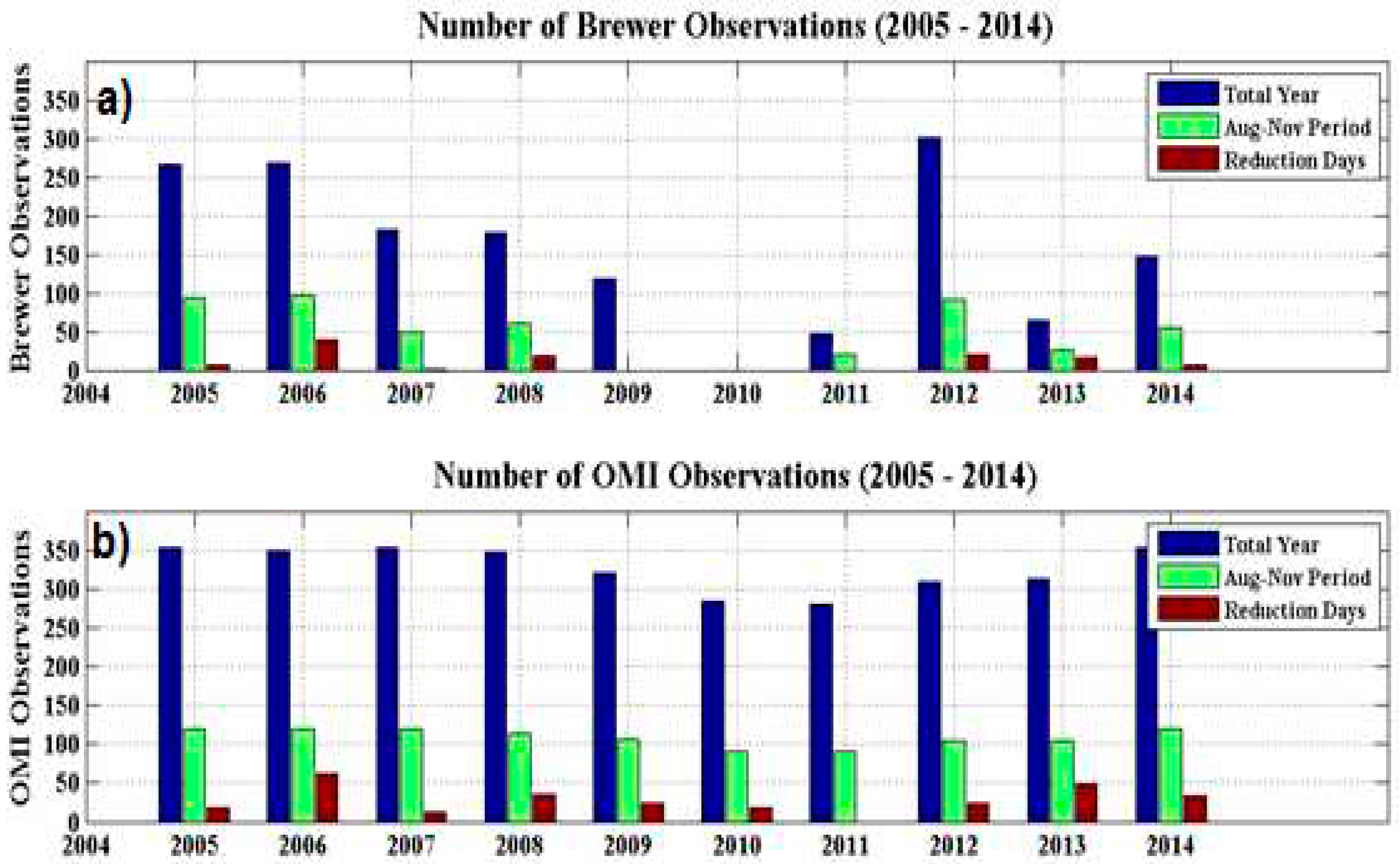
Figure 3.
(a) TOC of the BS #167 (gray) and OMI instrument satellite (brown) between August and November 2012. Values below -1.5σ limit (black star line) in blue (Brewer) and red (OMI satellite). (b) PV values for 670 K level (~ 24 km altitude) between August and November 2012. Dotted black line represents the climatology and dotted red line represents the +1.5σ PV values.
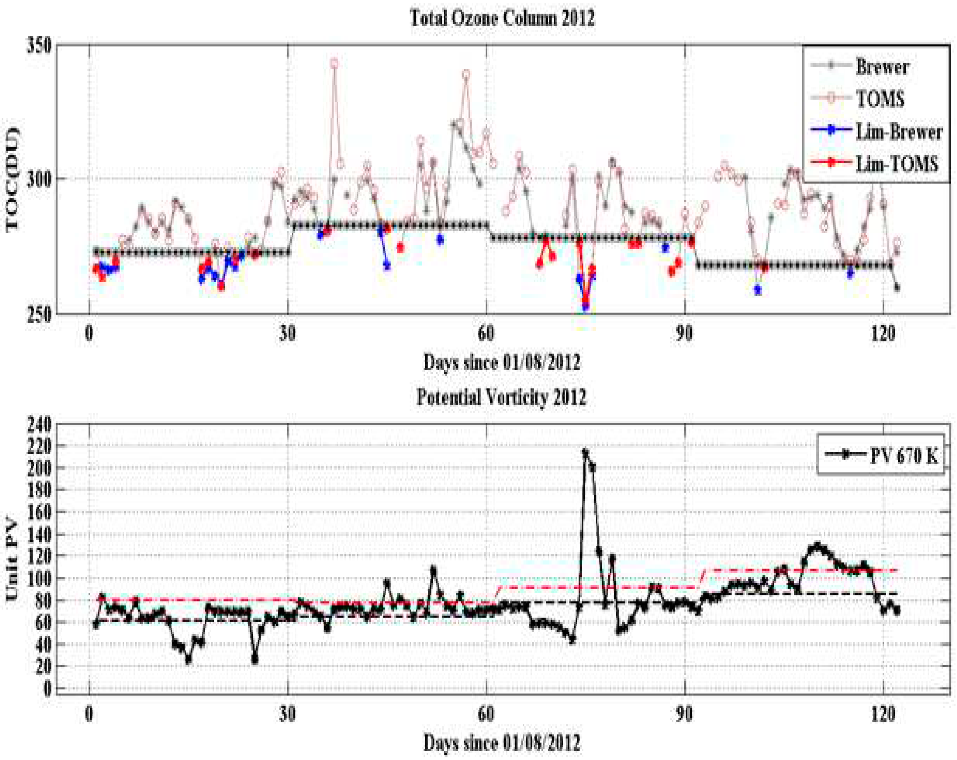
Figure 4.
(a) Comparison of the AURA/MLS satellite ozone profiles for October 14, 2012 in blue and October climatology ozone profile (black). Dotted lines correspond to ±1.5σ October climatology limit. (b) Percent ozone anomalies, derived as differences between monthly and daily ozone recorded on 10, 12, 14 and 16 October, 2012. Dotted black line represents the null difference.
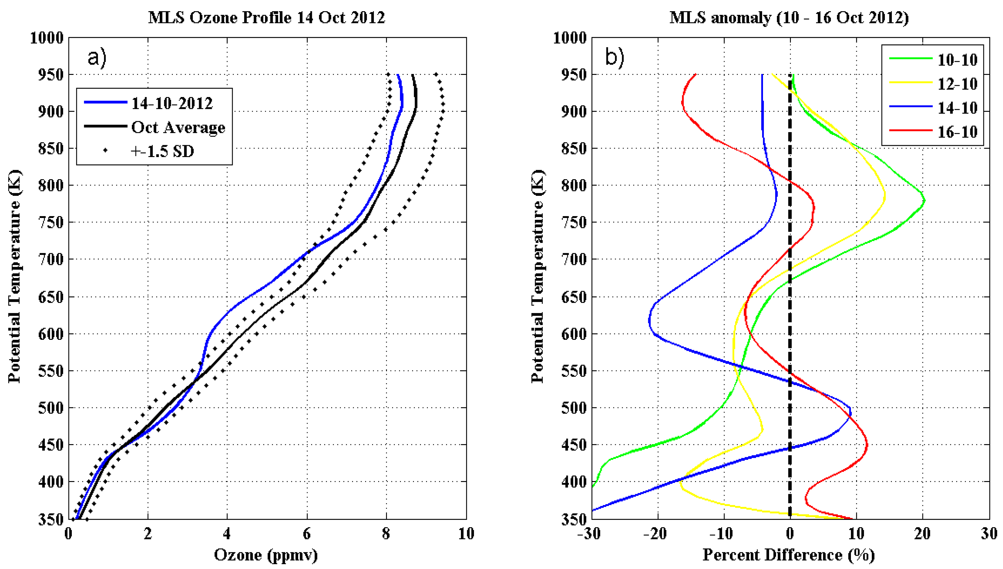
Figure 5.
Vertical evolution of the MIMOSA model PV fields in stratospheric isentropic surfaces (400, 450, 500, 525 675 and 850 K) on October 14, 2012. Locations of dynamical barriers (Subtropical barrier in red and polar barrier in black) are overlapped on the maps using a color scale with PV units. The X indicates the SSO location.
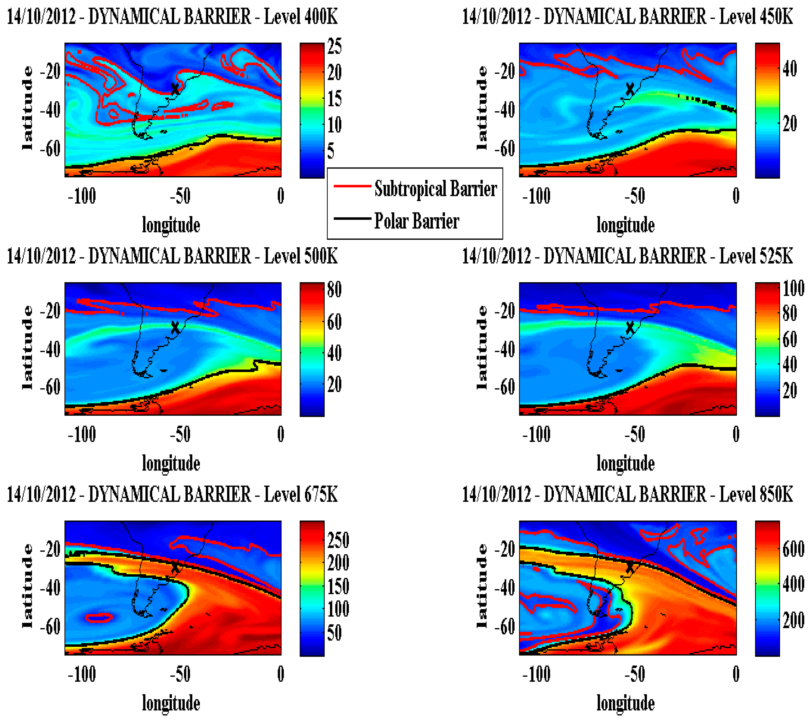
Figure 6.
Temporal evolution of MIMOSA model PV fields for 675 K isentropic surface obtained on 08, 10, 12, 14, 16 and 18 October 2012. Locations of dynamical barriers (Subtropical barrier in red and polar barrier in black) are overlapped on the maps using a color scale with PV units. The X indicates the SSO location.
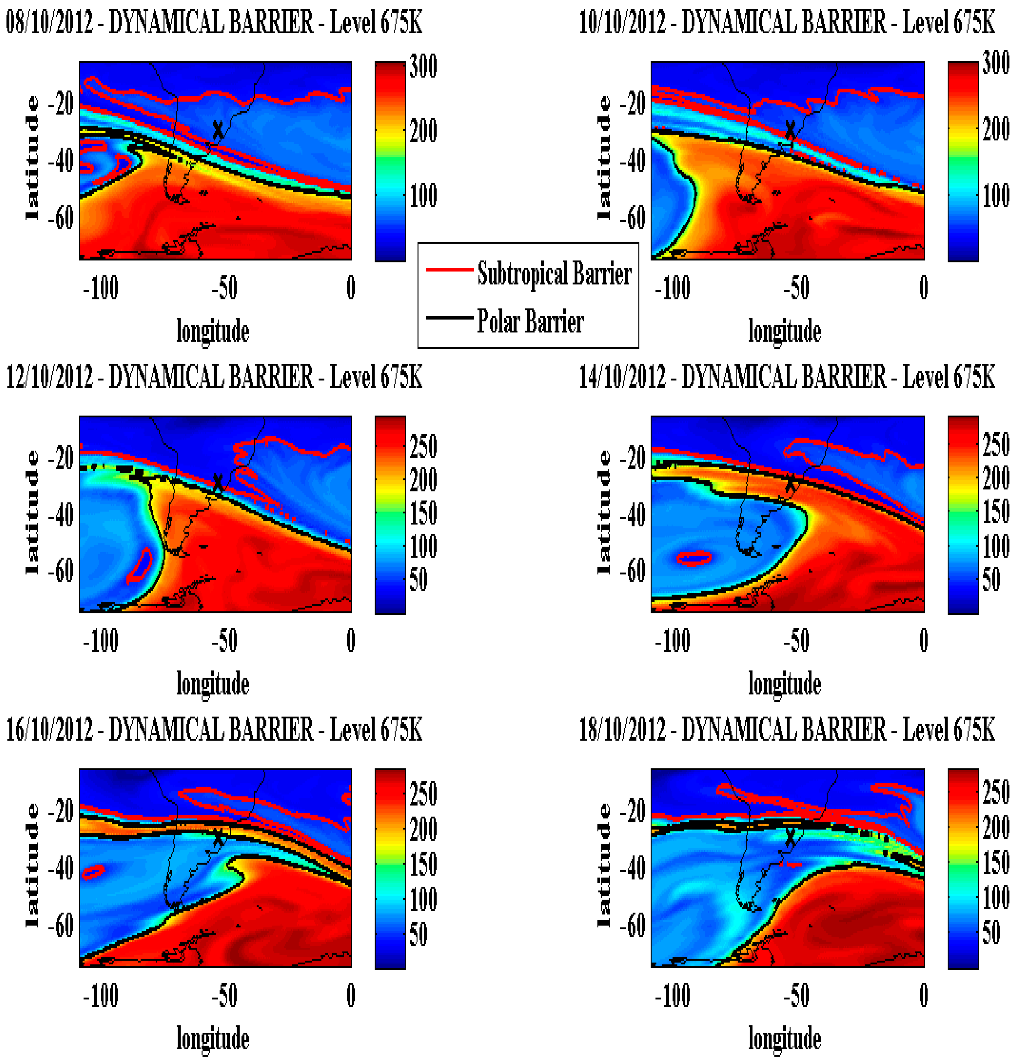
Figure 7.
Time distribution of the number of SBAOHI events per month and per year between 2005 and 2014.
Figure 7.
Time distribution of the number of SBAOHI events per month and per year between 2005 and 2014.
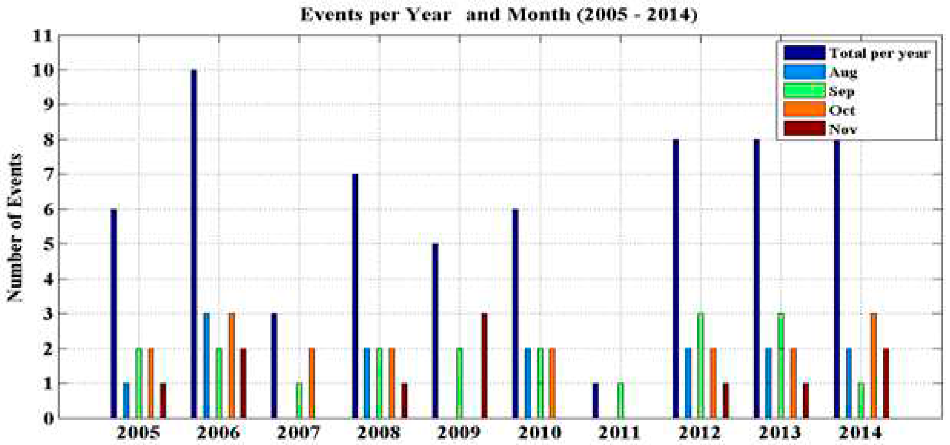
Figure 8.
Frequency of occurrence (percentage %) of SBAOHI events per month. The upper plots, (a) and (b), illustrate the events with a “tongue” structure statistics, while the lower plots, (c) and (d), present the “filament” structure events between 2005 and 2014.
Figure 8.
Frequency of occurrence (percentage %) of SBAOHI events per month. The upper plots, (a) and (b), illustrate the events with a “tongue” structure statistics, while the lower plots, (c) and (d), present the “filament” structure events between 2005 and 2014.
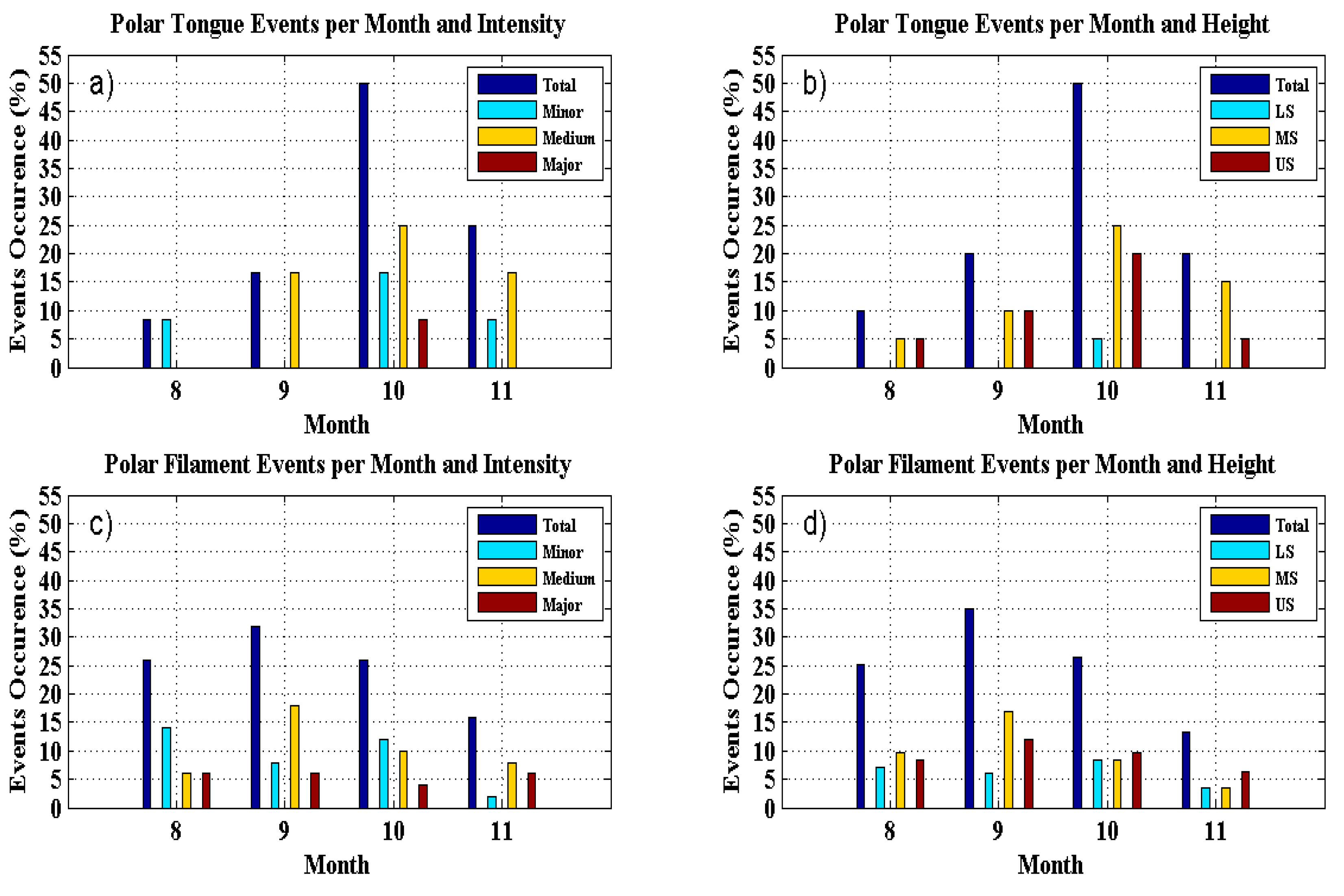
Figure 9.
Intensity of TOC reduction during the SBAOHI events between 2005 and 2014 compared to QBO (a) and ENSO (b) indices. Minor events (green), medium events (yellow), major events (red) and climatic indexes are presented by the black dashed line.
Figure 9.
Intensity of TOC reduction during the SBAOHI events between 2005 and 2014 compared to QBO (a) and ENSO (b) indices. Minor events (green), medium events (yellow), major events (red) and climatic indexes are presented by the black dashed line.
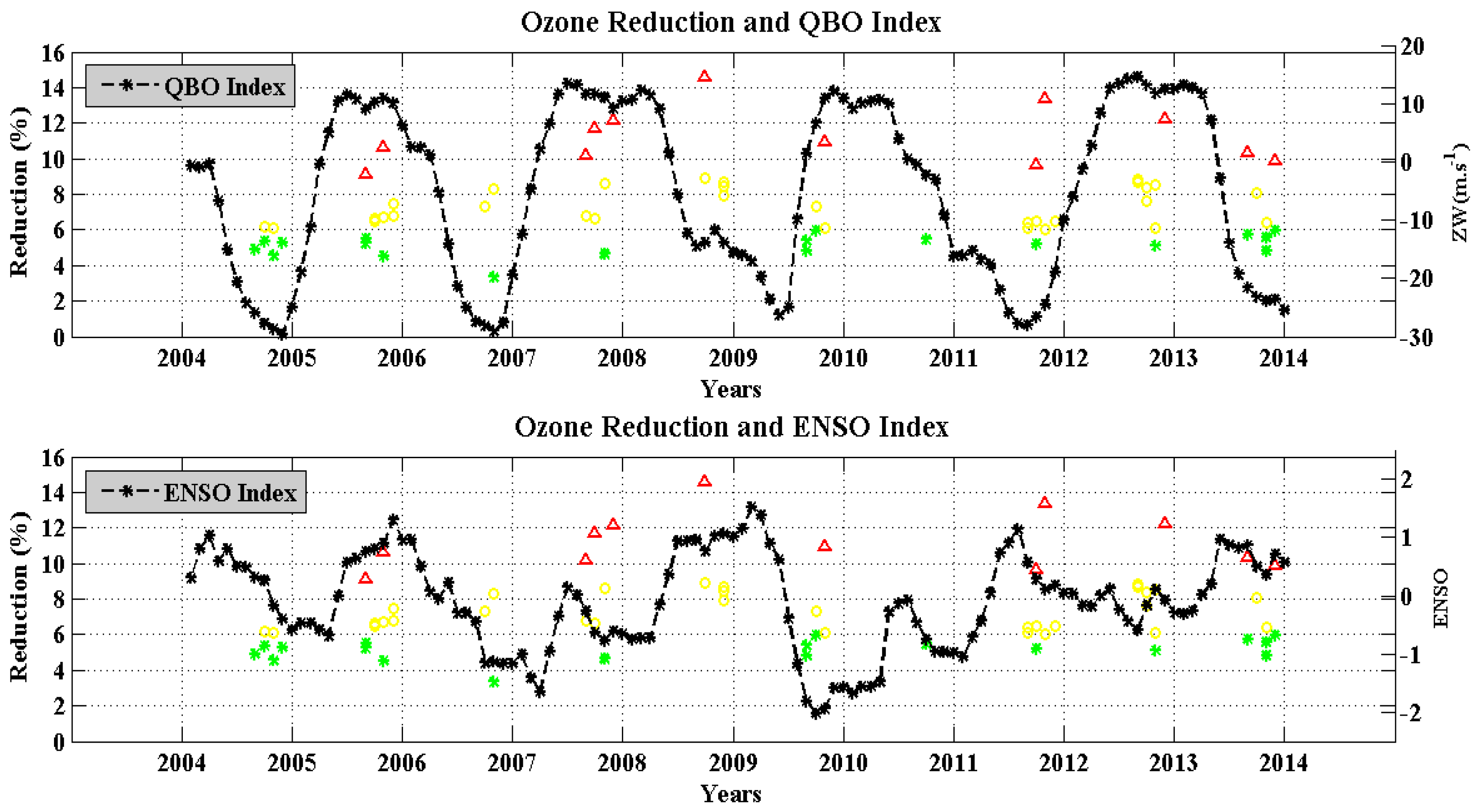

Table 1.
Climatological values, standard deviations (σ) and -1.5σ limit for the August-November period in SSO station.
Table 1.
Climatological values, standard deviations (σ) and -1.5σ limit for the August-November period in SSO station.
| Month | O3 Climatology in DU (µ) | O3 SD in DU (σ) | Limit -1.5σ in DU (µ-1.5σ) |
|---|---|---|---|
| August | 284.9 | 9.1 | 271.4 |
| September | 296.6 | 9.9 | 281.7 |
| October | 290.2 | 8.8 | 277.0 |
| November | 286.6 | 13.0 | 267.0 |
Disclaimer/Publisher’s Note: The statements, opinions and data contained in all publications are solely those of the individual author(s) and contributor(s) and not of MDPI and/or the editor(s). MDPI and/or the editor(s) disclaim responsibility for any injury to people or property resulting from any ideas, methods, instructions or products referred to in the content. |
© 2023 by the authors. Licensee MDPI, Basel, Switzerland. This article is an open access article distributed under the terms and conditions of the Creative Commons Attribution (CC BY) license (http://creativecommons.org/licenses/by/4.0/).
Copyright: This open access article is published under a Creative Commons CC BY 4.0 license, which permit the free download, distribution, and reuse, provided that the author and preprint are cited in any reuse.


