
Submitted:
07 August 2025
Posted:
11 August 2025
You are already at the latest version
Abstract
Angle crack defects significantly affect compressor blade radial deformation characteristics, posing critical challenges for reliability assessment under operational uncertainties. This study proposes a novel OOA-optimized Kriging-RBF (OOA-KR) method for efficient reliability evaluation of blade radial clearance with angle crack defects. The approach integrates Kriging's uncertainty quantification capabilities with RBF neural networks' nonlinear mapping strengths through an adaptive weighting scheme optimized by the Osprey Optimization Algorithm. Multiple uncertainty sources including crack geometry, operational temperature, and loading conditions are systematically considered. A comprehensive finite element model incorporating crack size variations and multi-physics coupling effects generates training data for surrogate model construction. Comparative studies demonstrate superior prediction accuracy with RMSE = 0.568 and R² = 0.8842, significantly outperforming conventional methods while maintaining computational efficiency. Reliability assessment achieves 97.6% precision through Monte Carlo simulation. Sensitivity analysis reveals rotational speed as the most influential factor (S = 0.42), followed by temperature and loading parameters. The proposed OOA-KR method provides an effective tool for blade design optimization and reliability-based maintenance strategies.
Keywords:
aeroengine
; compressor blade
; angle crack
; reliability assessment
; Kriging
; RBF
1. Introduction
Compressor blade radial deformation poses a critical design challenge in modern aeroengines, where precise tip clearance control directly influences aerodynamic efficiency, operational safety, and engine performance [1,2,3]. Under operational conditions, blades experience complex multi-physics loading, including centrifugal forces, aerodynamic pressures, thermal gradients, and vibratory excitations, resulting in intricate radial displacement patterns that must be carefully managed to prevent blade-casing contact while minimizing tip leakage losses [4,5]. Angle crack defects, which typically occur at blade tip corners due to stress concentration and high-cycle fatigue, significantly complicate this deformation behavior by introducing local compliance reductions, altered load paths, and time-dependent structural property changes [6,7]. These crack-induced effects create highly nonlinear relationships between operational parameters and radial clearance, necessitating sophisticated reliability assessment methodologies to ensure safe and efficient engine operation under uncertainty.
Traditional structural reliability assessment approaches for compressor blade systems predominantly rely on first-order reliability methods (FORM), second-order reliability methods (SORM), and Monte Carlo simulation techniques [8,9,10]. While FORM and SORM offer computational efficiency through linearization or quadratic approximation of limit state functions, they often fail to capture the complex nonlinear coupling effects inherent in crack-damaged blade structures, particularly when multiple uncertainty sources interact simultaneously [11,12]. Monte Carlo simulation provides accurate reliability estimates but requires extensive computational resources due to the need for repeated high-fidelity finite element analyses, making it impractical for design optimization and real-time monitoring applications. Furthermore, conventional reliability methods struggle with the multi-modal response surfaces and discontinuous behavior introduced by crack propagation, leading to inaccurate failure probability estimates and potentially unsafe design margins [13]. These limitations highlight the critical need for advanced computational approaches that can balance accuracy and efficiency in modeling crack-structure interactions, motivating the development of surrogate modeling techniques for reliability assessment of damaged blade systems.
Surrogate modeling techniques have emerged as promising alternatives to address computational challenges in structural reliability assessment, with Kriging, Gaussian Process (GP) models and Radial Basis Function (RBF) networks gaining particular attention for their interpolation capabilities and uncertainty quantification properties [14,15,16]. Su et al. proposed a GP-based dynamic surrogate model for complex engineering structural reliability analysis [17]. However, individual surrogate models exhibit inherent limitations when applied to crack-influenced blade deformation problems. GP models excel in uncertainty quantification and global trend capture but may struggle with sharp response transitions and discontinuities introduced by crack boundaries [18]. Conversely, RBF networks demonstrate superior nonlinear mapping capabilities and local approximation performance but provide limited uncertainty information essential for reliability analysis [19,20]. Chen et al. developed a multi-fidelity data aggregation using convolutional neural networks for multi-fidelity modeling [21]. Recent research efforts have explored hybrid surrogate modeling approaches to leverage complementary strengths of different metamodeling techniques. Wang et al. introduced a new adaptive extreme response surface approach for time-variant reliability problems [22]. Xia et al. developed a hybrid approach to seismic reliability assessment [23]. Additionally, Rabhi et al. proposed a combined a dynamic reliability method and a me-ta-model (reduced model) to obtain good results in the reliability and optimization of physical systems [24]. However, most existing hybrid schemes focus on simple ensemble averaging or sequential correction methods without addressing the specific challenges posed by crack-induced response characteristics.
Optimization algorithms play a crucial role in surrogate model parameter tuning and hybrid weight determination, with evolutionary algorithms, swarm intelligence methods, and gradient-based techniques being widely employed [25,26]. Traditional genetic algorithms and particle swarm optimization approaches often suffer from premature convergence and local optima entrapment when dealing with high-dimensional parameter spaces typical of hybrid surrogate models. Liu et al. developed an efficient reliability analysis framework for OST using the kriging model of optimal linear unbiased estimation [27]. More recent nature-inspired algorithms such as whale optimization, grey wolf optimization, and artificial bee colony algorithms have shown improved global search capabilities but may lack sufficient exploitation ability for fine-tuning complex hyperparameter configurations [28,29,30]. Liu et al. developed a method combining the shear strength reduction (SSR) technique, the surrogate model and the adaptive pool-based sampling strategy for efficient slope reliability analysis [31]. Kumar et al introduced a data-driven model approximating the relationship between the inputs and outputs by using an adaptive sparse polynomial chaos expansion approach [32]. Wong et al. developed a novel method considering the equality constraints, inequality and physical constraints of the hydro-thermal systems, which combined with simulated annealing, genetic algorithms, and two hybrid optimization techniques [33]. However, these conventional optimization algorithms still face significant limitations in handling the complex multi-modal landscapes characteristic of crack-damaged systems. The Osprey Optimization Algorithm (OOA) offers distinct advantages over traditional methods through its unique dual-phase search mechanism that combines aggressive exploration via high-altitude soaring behavior with precise exploitation through targeted diving strategies, enabling superior performance in navigating complex, multi-modal parameter spaces while maintaining computational efficiency [34]. Current optimization-based surrogate modeling approaches face two critical limitations: (1) poor exploration-exploitation balance in high-dimensional spaces, resulting in suboptimal configurations; and (2) insufficient efficiency and accuracy in optimization processes.
To address these challenges, this study proposes a novel OOA-optimized Kriging-RBF (OOA-KR) method for efficient reliability assessment of compressor blade radial clearance considering angle crack defects. The proposed approach integrates the uncertainty quantification capabilities of Kriging with the nonlinear mapping strengths of RBF neural networks through an adaptive weighting scheme optimized by the Osprey Optimization Algorithm (OOA). The OOA algorithm combines global exploration abilities inspired by osprey hunting behavior with local exploitation mechanisms derived from fish positioning dynamics, providing superior parameter optimization performance for hybrid surrogate model construction. Multiple uncertainty sources including crack geometry variations, operational temperature fluctuations, loading condition changes, and material property scatter are systematically incorporated to evaluate their effects on blade radial deformation distribution and reliability assessment accuracy.
2. OOA-Optimized Kriging-RBF Method (OOA-KR)
The proposed OOA-KR method represents a novel hybrid metamodeling approach that synergistically integrates the global modeling capability of Kriging with the local approximation advantages of RBF neural networks through an adaptive weighted fusion strategy. This hybrid framework leverages Kriging’s proficiency in uncertainty quantification and global trend modeling, while capitalizing on RBF’s superior performance in capturing nonlinear local features and handling high-dimensional scattered data. The key innovation lies in the simultaneous optimization of fusion weights and hyperparameters of both base models using the Osprey Optimization Algorithm (OOA), which combines the global exploration ability of eagle search behavior with the local exploitation capability of fish swarm dynamics. The overall framework of the proposed method is illustrated in Figure 1, demonstrating the complete workflow from data preprocessing to performance function modeling.
The mathematical formulation of the OOA-KR method can be expressed as:
where g1 (x) represents the Kriging surrogate model, g2(x) denotes the RBF neural network model, and λ1, λ2 are the adaptive fusion weights subject to the constraint λ1+λ2=1.
The OOA-KR method follows a systematic approach consisting of the following steps:
Step 1: Collect and preprocess the training dataset D={(xᵢ, yᵢ), i=1, 2, ..., n}, including data normalization, outlier detection, and quality assessment to ensure data integrity.
Step 2: Construct the Kriging surrogate model g₁(x) based on the training data, establishing optimal spatial correlation functions and estimating model parameters through maximum likelihood estimation.
Step 3: Build the RBF neural network surrogate model g₂(x) using the same training dataset, determining the optimal network architecture, basis function types, and center locations.
Step 4: Design the weighted fusion strategy Y(x) = λ₁g₁(x) + λ₂g₂(x) with the constraint λ₁+λ₂ = 1 to combine the predictions from both base models while maintaining prediction consistency.
Step 5: Define the multi-objective optimization function incorporating cross-validation error metrics (RMSE, R²) and model complexity penalties as the fitness function for OOA.
Step 6: Initialize OOA parameters including population size, maximum iterations, search space bounds, and algorithm control parameters for both osprey hunting and fish positioning phases.
Step 7: Execute OOA iterative optimization to simultaneously determine optimal fusion weights {λ₁, λ₂} and hyperparameters of both base models through bi-phase population update mechanisms.
Step 8: Construct the final optimized fusion surrogate model using the obtained optimal parameters and evaluate its performance on independent test datasets through comprehensive validation metrics.
2.1. Kriging
Kriging, originally developed by Krige for geostatistical applications, has emerged as a powerful metamodeling technique for approximating expensive computational models in engineering design and reliability analysis. Unlike polynomial-based response surface methods that rely on global fitting, kriging provides an interpolative approach that exactly reproduces the observed data while offering optimal predictions at unsampled locations with quantified uncertainty bounds.
The kriging metamodel treats the deterministic computer response as a realization of a stochastic process, expressed mathematically as [14]:
where g1(x) represents the unknown function of interest, f(x)=[f1(x), f2(x), …, fp(x)]T denotes a vector of known regression functions, β=[β1, β2, …, βp] is the vector of regression coefficients, and Z(x) represents a zero-mean Gaussian random process with covariance structure:
where term fT(x)β captures the global trend of the response surface, while Z(x) models the local deviations to ensure interpolation through the training data points.
Given a set of n training points {x(1), x(2), …, x(n)} and their corresponding responses {y(1), y(2), …, y(n)}, the unknown parameters are estimated using maximum likelihood estimation:
where F is n×p regression matrix with elements Fij=f(xi), R is the n×n correlation matrix with elements R=R(xi, xj), and y=[ y(1), y(2), …, y(n)].
The correlation function R(xi, xj) governs the smoothness and local behavior of the metamodel. Commonly employed correlation functions include the exponential, Gaussian, and Matérn families. For multivariate inputs, a separable correlation structure is typically assumed:
where d is the input dimension and R represents the correlation function.
The kriging predictor at an arbitrary point x is given by:
2.2. RPF
Radial basis function (RBF) networks represent a class of neural network architectures that have gained considerable attention in engineering metamodeling due to their universal approximation capabilities and relatively simple mathematical formulation. Unlike traditional feedforward neural networks, RBF networks employ radially symmetric basis functions that provide localized responses, making them particularly suitable for interpolating scattered data in high-dimensional spaces.
The RBF metamodel approximates an unknown function y(x) as a linear combination of radial basis functions [16]:
where wi represents the weight associated with the i-th basis function, ϕ(⋅) denotes the radial basis function, ci are the center locations(typically coinciding with training points), ‖⋅‖ represents the Euclidean norm, and p(x) is an optional polynomial term to ensure well-posedness.
Common types of RBF include the Gaussian function:
where ε is a shape parameter controlling the width of the basic functions.
2.3. OOA -Optimized Weighted Fusion and Hyper-Parameter Solution
The OOA-KR method formulates the hyperparameter optimization as a multi-dimensional problem where the decision variables Θ include fusion weights {λ₁, λ₂}, Kriging parameters {θk}, and RBF parameters {ε, ci, wi}. The objective function balances prediction accuracy and model generalization:
Similar to other optimization algorithms, the population is randomly initialized in the optimization space:
where xi,j is index individuals; lbj is the lower bound of the search space for variable j; ubj is the upper bound; r is a random number uniformly distributed in the interval [0,1].
The osprey is a powerful hunter. Due to its strong eyesight, it can detect the position of underwater fish. After determining the fish’s location, they attacked it and hunted for it underwater. The first stage of population update in OOA is modeled based on the simulation of the natural behavior of ospreys. Modeling the fish attacked by ospreys can lead to significant changes in the ospreys’ positions in the search space, which enhances the exploration ability of OOA in identifying the best areas and escaping local optima.
In OOA design, for each osprey, the positions of other ospreys with better objective function values in the search space are regarded as underwater fish. The fish group for each osprey is specified by
where FPi is the fish set of the i-th osprey, and Xbest is the best position for the osprey.
The osprey randomly detected the position of one of the fish and attacked it. Based on the simulation of the osprey’s movement towards the fish, the new position of the corresponding osprey is calculated using Eq. (13). If the new position is better, replace the osprey’s previous position according to Eq. (14)
wherein SF is the fish selected by the osprey, r is a random number between 0 and 1, and the value of I is one of {1,2}.
After hunting a fish, an osprey will take it to a suitable (safe) location where it eats. The second stage of population update in OO 8 is based on modeling the simulation of the natural behavior of ospreys. Modeling that brings the fish to the right position leads to minor changes in the osprey’s position in the search space, which increases the utilization ability of OOA in local search and conversions to better solutions near the discovered ones.
In the design of OOA, to simulate this natural behavior of ospreys, first of all, for each member of the population, a new random position is calculated using Eq. (15) as the “position suitable for eating fish”. Then, if the value of the objective function is improved at this new position, it replaces the previous position of the corresponding osprey according to Eq. (16).
Here, t is the number of iterations, and T is the maximum number of iterations.
The OOA algorithm optimizes the fusion weights and hyperparameters through the following systematic steps:
Step 1: Initialize osprey population with random parameter vectors within predefined bounds, ensuring each individual represents a complete set of fusion weights and model hyperparameters.
Step 2: Evaluate fitness of each individual by constructing Kriging and RBF models with corresponding hyperparameters, computing fusion predictions, and calculating cross-validation error metrics.
Step 3: Identify the fish population for each osprey based on fitness ranking, where better-performing individuals serve as potential targets for position updates.
Step 4: Hunting phase by updating osprey positions through simulated fish attack behavior, promoting global exploration of the parameter space.
Step 5: Feeding phase by fine-tuning osprey positions through local search mechanisms, enhancing exploitation of promising regions.
Step 6: Update population by replacing inferior solutions with improved ones, maintaining diversity while progressing toward optimal parameter configurations.
Step 7: Check convergence criteria (maximum iterations, fitness threshold, or population stagnation) and terminate if satisfied, otherwise return to Step 2.
Step 8: Extract optimal fusion weights and hyperparameters from the best individual, construct the final OOA-KR model, and validate performance on test data.
The algorithm of OOA-KR is shown as follows: 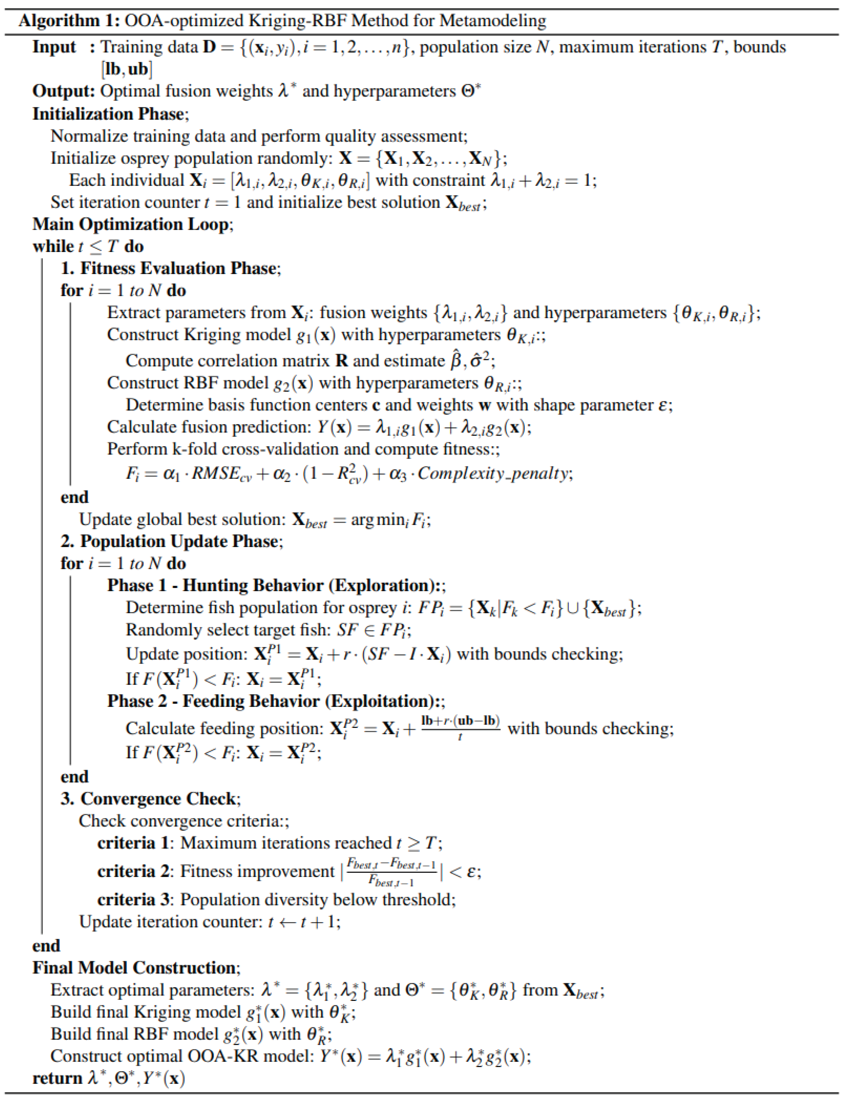
3. Structural Reliability Assessment of Compressor Blade Angle Crack Based on OOA-KR Method
Reliability theory is an important tool to deal with uncertainty in the design and evaluation of engineering structures. The core of structural reliability analysis is to quantify the failure probability, that is, the probability that the structure fails to meet the performance requirements under the given random variable conditions, as shown in Figure 2.
For compressor blade radial clearance deformation, the failure probability Pf is expressed by
where g(X) is the limit state function; g(X)≤0 stands for structural security boundary; f(x) is the joint probability density function of random variables.
The limit state function for compressor blade radial clearance deformation is defined as [1,3]:
where δallow represents the maximum allowable radial clearance deformation and δradial(x) is the actual radial clearance deformation, where g(x)≥0 indicates that the blade radial clearance is within the safe range and g(x)<0 indicates structural failure.
Since the limit state function (LSF) is usually highly nonlinear, the direct calculation of failure probability will consume a lot of computing resources. Monte Carlo (MC) simulation estimates the probability of failure by random sampling, and its basic idea is to calculate failure events through a large number of samples. Specifically, the failure probability can be expressed as:
In this paper, MC simulation is used to determine the radial clearance deformation distribution of compressor blades, and hence, the reliability degree is expressed as
in which R is the degree of reliability; I(·) is the indicator function of the margin of safety; Nr is the number of samples located in the margin of safety; and N indicates the number of total samples.
The sensitivity index Si and importance index Ii are defined as
where xi is the value of the i-th input parameter; µi is the mean value of the i-th samples; β is a normalizing factor for the sensitivities; Sd,i is the sensitivity index of the i-th samples; and m is the total number of input samples.
4. Experiments and Results
4.1. Experiment Environment
The experimental setup utilized a workstation featuring an Intel 13000KF processor, NVIDIA GeForce RTX 4090 graphics card, 64 GB memory, and 2 TB NVMe solid-state drive for rapid data retrieval. The computing environment operated on Windows 11 with Python 3.9 deployed through Anaconda distribution.
4.2. Deterministic Simulation of Blade with Angle Crack
A comprehensive three-dimensional finite element model of the compressor blade with angle crack defects was established. The angle crack is located at the intersection between the blade tip edge and the suction, where complex multiaxial stress states occur during operation, including centrifugal tension, aerodynamic bending loads, and thermal gradients. Cracks of varying lengths are simulated by adjusting the contact mode between the diminutive triangular blade block and the remaining blade structure. The spatial relationship between these small triangular blade blocks and the intact blade segments is illustrated in Figure 3(a), while the mesh configuration employed in the simulation is depicted in Figure 3(b). For blade model with angle crack, the number of nodes and cells for remaining blade and small triangular blades are, 12,315 and 8,321, and 1,273 and 963, respectively.
The simulation of the angular crack is achieved by manipulating the contact approach. A binding contact is established on a no-crack surface, while a frictionless contact is implemented directly at the crack surface. The length and position of the crack are controlled by altering the relative placement of binding and frictionless. To enhance the simulation efficiency, the crack surface is subdivided into some cells, as shown in Figure 4. Frictionless contact is applied between some cells surface on the triangular blade and the upper contact surface of remaining blade, while binding contact is employed for the other cell surfaces of the triangular blade.
This study examines a turbine compressor blade with constrained root conditions, accounting for centrifugal forces generated by high-speed rotation. Figure 5 shows the geometric structure and boundary conditions of the turbine blade. Convective heat transfer boundaries are applied across four distinct regions: root, lower, middle, upper sections, and tip area. Each region is characterized by specific temperature values (T1, T2, T3, T4) and corresponding heat transfer coefficients (a1, a2, a3, a4). Nine stochastic parameters follow normal distribution patterns, detailed in Table 1, with numerical designation 1-4 representing exterior-to-interior positioning. Besides, the distribution of crack lengths is included in Table 1. Finite element modeling incorporates these boundary specifications, yielding results presented in Figure 6 that serve as baseline data for subsequent reliability assessment.
4.3. Structural Reliability Assessment of Compressor Blade Angle Crack
As shown in Table 2, it is the relationship between Monte Carlo simulation sample sizes and reliability degrees. As the MCS increases from 102 to 105, the reliability improves from 0.9512 to 0.9713, indicating convergence around 0.9713 when sample sizes reach 10⁴ and above. This demonstrates that larger sample sizes yield more stable reliability estimates.
Based on the probability distribution of input parameters, MC simulation is used to input 104 sets of randomized parameters into the established radial deformation analysis model to obtain clearance distribution. The obtained radial deformation is displayed in Figure 7, which follows a normal distribution with a mean value of 0.735 mm and a standard deviation of 0.037 mm. Figure 8 shows the distribution characteristics of the samples.
Table 3 quantifies the sensitivity indices (S) and importance indices (I) for ten critical parameters. Parameter 1 (ω) exhibits the highest sensitivity (S=0.42) and importance (I = 0.37), confirming rotational torque as the most influential factor. Parameters 2, 6, and 10 demonstrate moderate-to-high sensitivity values (S=0.36-0.39), while parameters 5, 8, and 9 show relatively low sensitivity (S=0.09-0.17). Figure 9 visualizes the sensitivity index distribution across all parameters, with color-coded bars representing different parameter categories. The results establish a clear hierarchy: high-sensitivity parameters (ω, T1), moderate-sensitivity parameters (T2, T3, σ1, σ2), and low-sensitivity parameters (ε3, ε4). This quantitative ranking provides essential guidance for design optimization and manufacturing tolerance allocation in fatigue life prediction applications.
4.4. Modeling Efficiency and Precision Analysis
Training data were generated using Latin Hypercube Sampling (LHS) to ensure uniform coverage across the multi-dimensional uncertainty parameter space. A total of 300 training samples were generated, with each sample corresponding to a complete multi-physics finite element analysis calculating the blade’s radial deformation response under specific parameter combinations. Data preprocessing included normalization of all input variables to [0,1] interval, outlier detection using 3σ criterion, and dataset partitioning with 7:2:1 ratio for training, validation, and testing sets.
The error metrics are used in this paper, including Root Mean Square Error (RMSE), Mean Absolute Error (MAE) and Coefficient of Determination (R2), which are defined as follows [3]:
where yi is the i-th radial deformation of true samples; n is total number of samples; ŷi is predicted value of the response variable for the i-th observation; ȳ is arithmetic mean of all measured values.
Table 4 presents a comprehensive performance comparison of different surrogate models across multiple evaluation metrics. The proposed OOA-KR method demonstrates superior performance with the highest R² value of 0.8842 and the lowest prediction errors (RMSE: 0.568, MAE: 0.412). Among the baseline methods, PSO-Kriging achieves the best performance (R²: 0.8616), followed by GA-Kriging (R²: 0.8445) and Kriging (R²: 0.8313), while ANN shows the poorest accuracy (R²: 0.6723). Regarding computational efficiency, basic methods (RBF, Kriging) require minimal training time (6.28-8.94s), whereas optimization-based approaches demand significantly longer training periods (52.82-88.31s) due to their iterative search processes. All models exhibit fast prediction times (0.013-0.043s), making them suitable for real-time applications. The results indicate that the proposed OOA-KR method achieves an optimal balance between prediction accuracy and computational efficiency.
Table 5 demonstrates the simulation precision of reliability estimation across different sample sizes. The proposed OOA-KR method achieves the highest simulation precisions of 91.9%, 96.3%, and 97.6% for sample sizes of 10², 10³, and 10⁴, respectively, significantly outperforming baseline methods. Among conventional approaches, PSO-Kriging exhibits the best performance (87.9%-90.7%), while ANN shows the lowest accuracy (69.7%-76.4%). All methods demonstrate improved precision with increasing sample sizes, with the proposed OOA-KR method maintaining superior performance across all sample configurations, indicating its effectiveness for reliability assessment applications.
5. Conclusions
This study proposes a novel OOA-optimized Kriging-RBF (OOA-KR) method for efficient reliability assessment of compressor blade radial clearance considering angle crack defects. The comprehensive investigation leads to the following key conclusions:
(1) Angle cracks significantly alter blade structural behavior, with crack simulation achieved through contact manipulation between triangular blade blocks and remaining structures, effectively capturing crack-induced compliance changes.
(2) The proposed OOA-KR hybrid model achieves superior prediction accuracy (RMSE=0.568, R²=0.8842), outperforming individual Kriging, RBF, and other optimization-based surrogate models by significant margins.
(3) Under normal operational conditions, the blade achieves a reliability of 0.9713 with mean radial deformation of 0.735 mm and standard deviation of 0.037 mm based on Monte Carlo simulation with 10⁴ samples.
(4) Global sensitivity analysis identifies rotational speed as the most critical factor (S=0.42, I=0.37), followed by temperature parameters and heat transfer coefficients, providing quantitative guidance for design priorities.
(5) The OOA-KR method demonstrates excellent computational efficiency with training time of 52.82s and prediction time of 0.025s, achieving optimal balance between accuracy and computational cost.
(6) The methodology achieves reliability assessment precision up to 97.6% for large sample sizes, significantly superior to conventional approaches and suitable for practical engineering applications.
The proposed approach demonstrates superior performance in capturing nonlinear multi-physics effects while maintaining computational efficiency, making it valuable for aerospace reliability applications. Future work will focus on extending the methodology to dynamic loading conditions and multiple crack interaction scenarios.
Author Contributions
Conceptualization, Q.Z. and S.-G.Z.; methodology,X.-Y.H.; software, Q.Z.; validation, Q.Z. and X.-Y.H.; formal analysis, Q.Z. and S.-G.Z.; investigation, Q.Z. and S.-G.Z.; resources, X.-Y.H.; data curation, Q.Z.; writing—original draft preparation, Q.Z.; writing—review and editing, X.-Y.H.;visualization,X.-Y.H.;supervision,S.-G.Z.;project administration,Q.Z.; funding acquisition, Q.Z. All authors have read and agreed to the published version of the manuscript.
Funding
This paper is Supported by the Open Research Subject of Engineering Research Center of Intelligent Space Ground Integration Vehicle and Control(Xihua University), Ministry of Education (grant number ZNKD2024-001)). The authors would like to thank it.
Data Availability Statement
The data used to support the findings of this study are included within the article.
Conflicts of Interest
The authors declare no conflicts of interest in publication.
References
- Wen, J. , Zheng, B. and Fei, C., 2025. Prioritized experience replay-based adaptive hybrid method for aerospace structural reliability analysis. Aerospace Science and Technology, 110257.
- Sun, H.O., Ren, A., Wang, Y., Zhang, M. and Sun, T., Deformation and vibration analysis of compressor rotor blades based on fluid-structure coupling. Engineering Failure Analysis 2021, 122, 105216. [CrossRef]
- Fei, C.W., Han, Y.J., Wen, J.R., Li, C., Han, L. and Choy, Y.S., Deep learning-based modeling method for probabilistic LCF life prediction of turbine blisk. Propulsion and Power Research 2024, 13, 12–25. [CrossRef]
- Benini, E., Biollo, R. and Ponza, R., Efficiency enhancement in transonic compressor rotor blades using synthetic jets: A numerical investigation. Applied Energy 2011, 88, 953–962. [CrossRef]
- Xu, D., Dong, X., Zhou, C., Sun, D., Gui, X. and Sun, X., Effect of rotor axial blade loading distribution on compressor stability. Aerospace Science and Technology 2021, 119, 107230. [CrossRef]
- Barlow, K.W. and Chandra, R., Fatigue crack propagation simulation in an aircraft engine fan blade attachment. International Journal of Fatigue 2005, 27, 1661–1668. [CrossRef]
- Poursaeidi, E., Sigaroodi, M.J. and Aieneravaie, M., Failure investigation of fatigue crack initiation and propagation in compressor blade. Engineering Failure Analysis 2024, 162, 108370. [CrossRef]
- Sankararaman, S., Daigle, M.J. and Goebel, K., Uncertainty quantification in remaining useful life prediction using first-order reliability methods. IEEE Transactions on Reliability 2014, 63, 603–619. [CrossRef]
- Karamchandani, A. and Cornell, C.A., Sensitivity estimation within first and second order reliability methods. Structural Safety 1992, 11, 95–107. [CrossRef]
- Zhen, H.S., Cheung, C.S., Leung, C.W. and Choy, Y.S., A comparison of the emission and impingement heat transfer of LPG–H2 and CH4–H2 premixed flames. International journal of hydrogen energy 2012, 37, 10947–10955. [CrossRef]
- Shao, B., Fan, C., Fu, S. and Zeng, J., Analysis of the Nonlinear Complex Response of Cracked Blades at Variable Rotational Speeds. Machines 2024, 12, 725. [CrossRef]
- Sun, Y.P., Wen, J.R., Li, J., Cao, A.F. and Fei, C.W., Novel Integrated Model Approach for High Cycle Fatigue Life and Reliability Assessment of Helicopter Flange Structures. Aerospace 2025, 12, 78. [CrossRef]
- Echard, B. , Gayton, N., Lemaire, M., Afzali, M., Bignonnet, A., Boucard, P.A., Defaux, G., Dulong, J.L., Ghouali, A., Lefebvre, F. and Pyre, A., Reliability assessment of an aerospace component subjected to fatigue loadings: APPRoFi project. 4th Fatigue Design 2013, 105-109.
- Sun, Z., Wang, J., Li, R. and Tong, C., LIF: A new Kriging based learning function and its application to structural reliability analysis. Reliability Engineering & System Safety 2017, 157, 152–165.
- Saida, T. and Nishio, M., Transfer learning Gaussian process regression surrogate model with explainability for structural reliability analysis under variation in uncertainties. Computers & Structures 2023, 281, 107014.
- Hong, L., Li, H. and Peng, K., A combined radial basis function and adaptive sequential sampling method for structural reliability analysis. Applied Mathematical Modelling 2021, 90, 375–393. [CrossRef]
- Su, G. , Peng, L. and Hu, L., A Gaussian process-based dynamic surrogate model for complex engineering structural reliability analysis. Structural Safety 2017, 68, 97–109. [Google Scholar] [CrossRef]
- Gramacy, R.B. and Lee, H.K.H., Bayesian treed Gaussian process models with an application to computer modeling. Journal of the American Statistical Association 2008, 103, 1119–1130. [CrossRef]
- Junior, F.E. and Almeida, I.F., Machine learning RBF-based surrogate models for uncertainty quantification of age and time-dependent fracture mechanics. Engineering Fracture Mechanics 2021, 258, 108037. [CrossRef]
- Duraisamy, K. , Zhang, Z.J. and Singh, A.P., New approaches in turbulence and transition modeling using data-driven techniques. In 53rd AIAA Aerospace sciences meeting 2015, 1284.
- Chen, J., Gao, Y. and Liu, Y., Multi-fidelity data aggregation using convolutional neural networks. Computer methods in applied mechanics and engineering 2022, 391, 114490. [CrossRef]
- Wang, Z. and Chen, W., Confidence-based adaptive extreme response surface for time-variant reliability analysis under random excitation. Structural Safety 2017, 64, 76–86. [CrossRef]
- Xia, Z., Quek, S.T., Li, A., Li, J. and Duan, M., Hybrid approach to seismic reliability assessment of engineering structures. Engineering Structures 2017, 153, 665–673. [CrossRef]
- Rabhi, N., Guedri, M., Hassis, H. and Bouhaddi, N., Structure dynamic reliability: A hybrid approach and robust meta-models. Mechanical systems and signal processing 2011, 25, 2313–2323. [CrossRef]
- Song, Z. , Wang, H., Xue, B., Zhang, M. and Jin, Y., 2023. Balancing objective optimization and constraint satisfaction in expensive constrained evolutionary multi-objective optimization. IEEE Transactions on Evolutionary Computation.
- Wei, F.F., Chen, W.N., Li, Q., Jeon, S.W. and Zhang, J., Distributed and expensive evolutionary constrained optimization with on-demand evaluation. IEEE Transactions on Evolutionary Computation 2022, 27, 671–685.
- Liu, P., Shang, D., Liu, Q., Yi, Z. and Wei, K., Kriging model for reliability analysis of the offshore steel trestle subjected to wave and current loads. Journal of Marine Science and Engineering 2021, 10, 25. [CrossRef]
- Nadimi-Shahraki, M.H., Zamani, H., Asghari Varzaneh, Z. and Mirjalili, S., A systematic review of the whale optimization algorithm: theoretical foundation, improvements, and hybridizations. Archives of Computational Methods in Engineering 2023, 30, 4113–4159. [CrossRef]
- Mirjalili, S., Mirjalili, S.M. and Lewis, A., Grey wolf optimizer. Advances in engineering software 2014, 69, 46–61. [CrossRef]
- Karaboga, D. and Akay, B., A comparative study of artificial bee colony algorithm. Applied mathematics and computation 2009, 214, 108–132. [CrossRef]
- Liu, Y., Li, X., Liu, X. and Yang, Z., A combined shear strength reduction and surrogate model method for efficient reliability analysis of slopes. Computers and Geotechnics 2022, 152, 105021. [CrossRef]
- Kumar, D., Koutsawa, Y., Rauchs, G., Marchi, M., Kavka, C. and Belouettar, S., Efficient uncertainty quantification and management in the early stage design of composite applications. Composite structures 2020, 251, 112538. [CrossRef]
- Wong, S.Y.W., Hybrid simulated annealing/genetic algorithm approach to short-term hydro-thermal scheduling with multiple thermal plants. International journal of electrical power & energy systems 2001, 23, 565–575.
- Yuan, Y., Yang, Q., Ren, J., Mu, X., Wang, Z., Shen, Q. and Zhao, W., Attack-defense strategy assisted osprey optimization algorithm for PEMFC parameters identification. Renewable Energy 2024, 225, 120211. [CrossRef]
Figure 1.
The framework of proposed OOA-HR method for surrogate modeling.
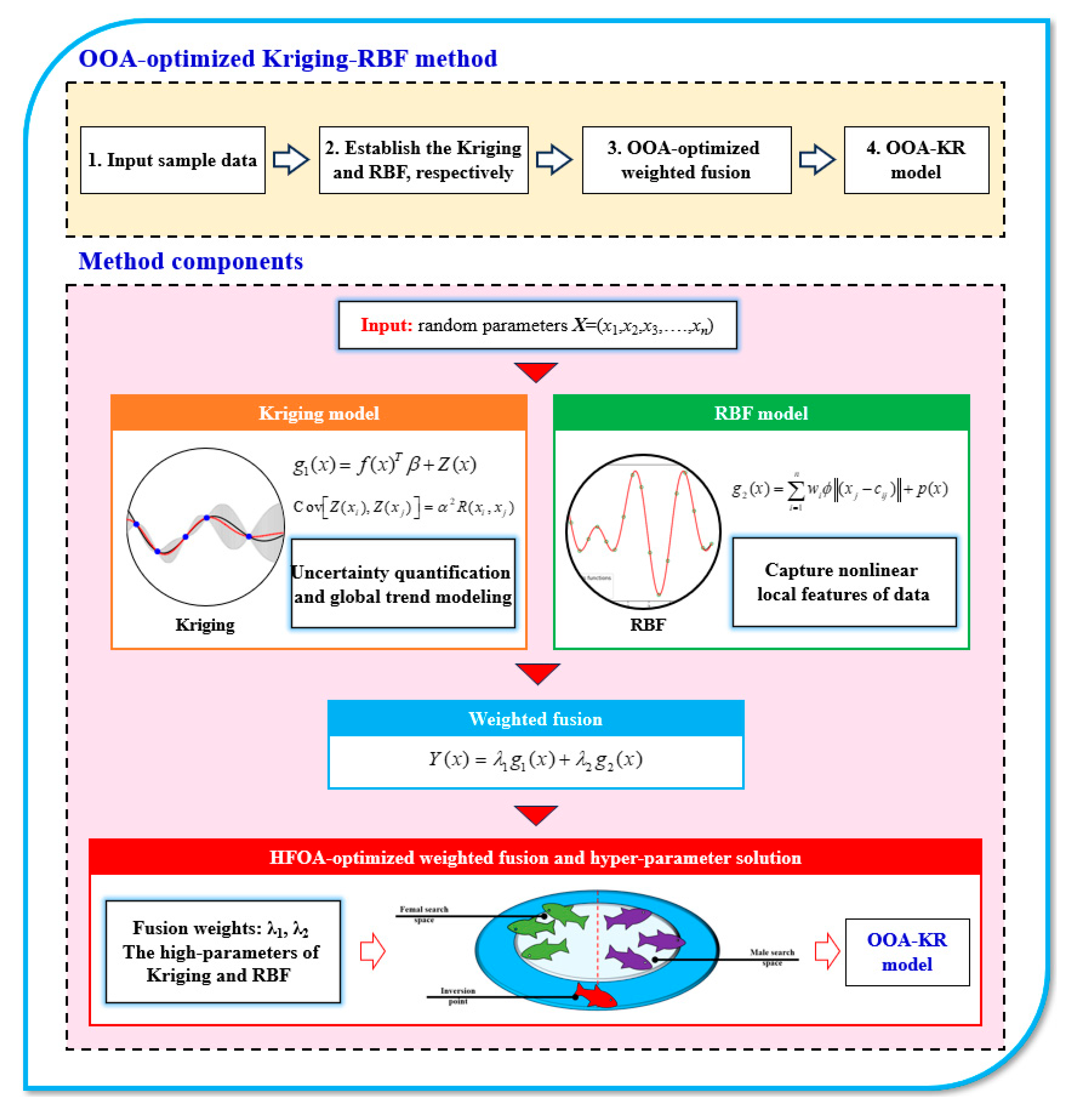
Figure 2.
The framework of OOA-KR method for structural reliability analysis.
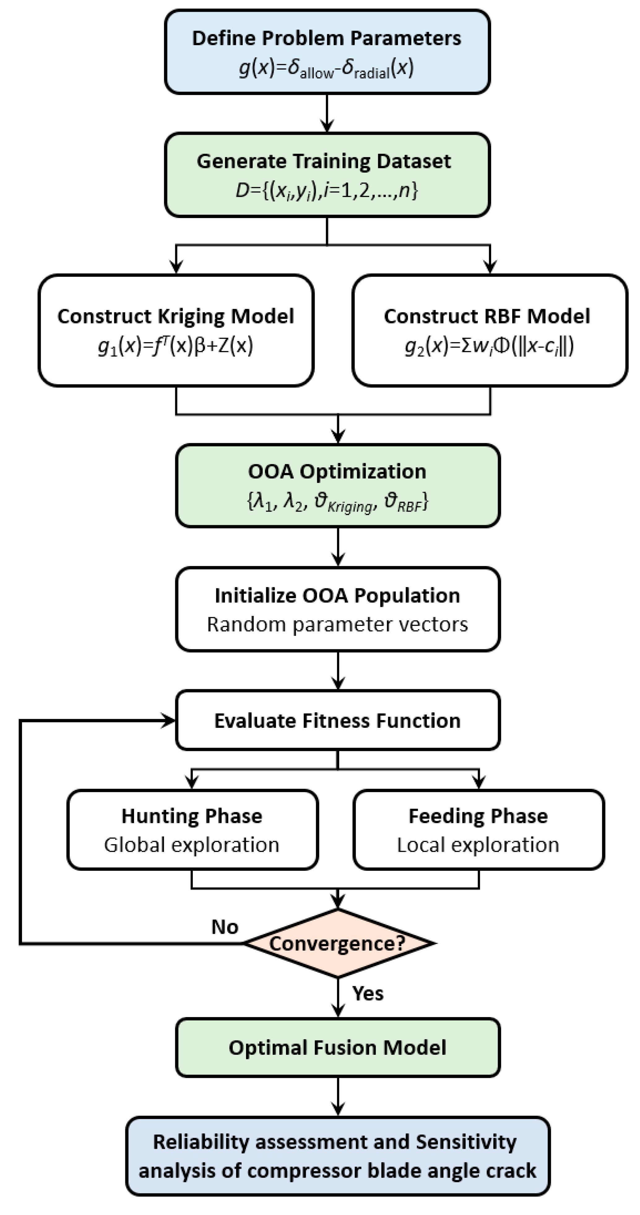
Figure 3.
Blade model with angle crack.
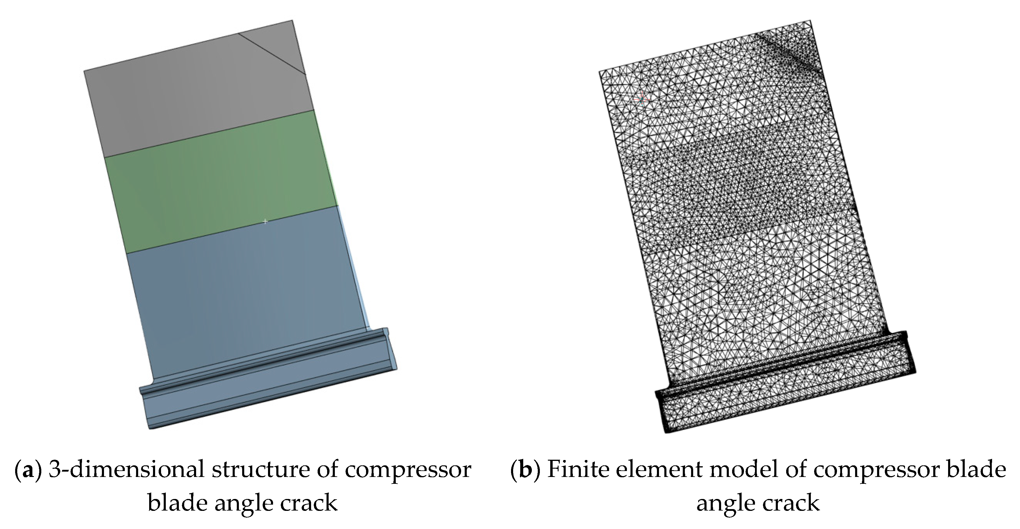
Figure 4.
Equal graph of crack surface.
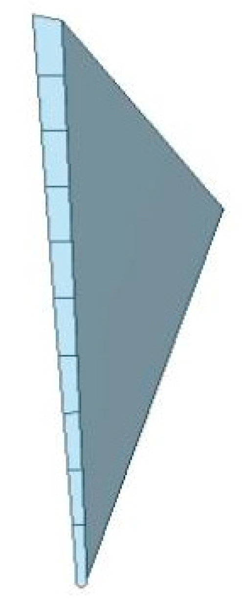
Figure 5.
3-dimentional geometry and boundary conditions of turbine blade.
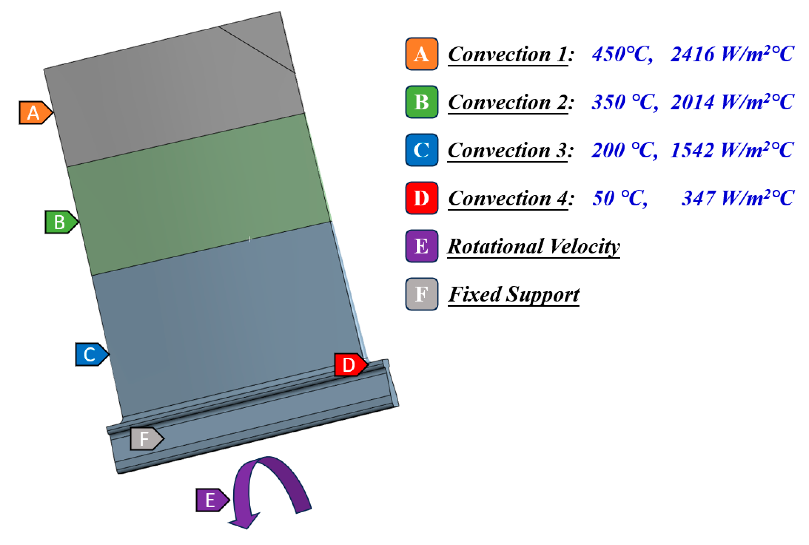
Figure 6.
The radial deformation analysis result of compressor blade angle crack.
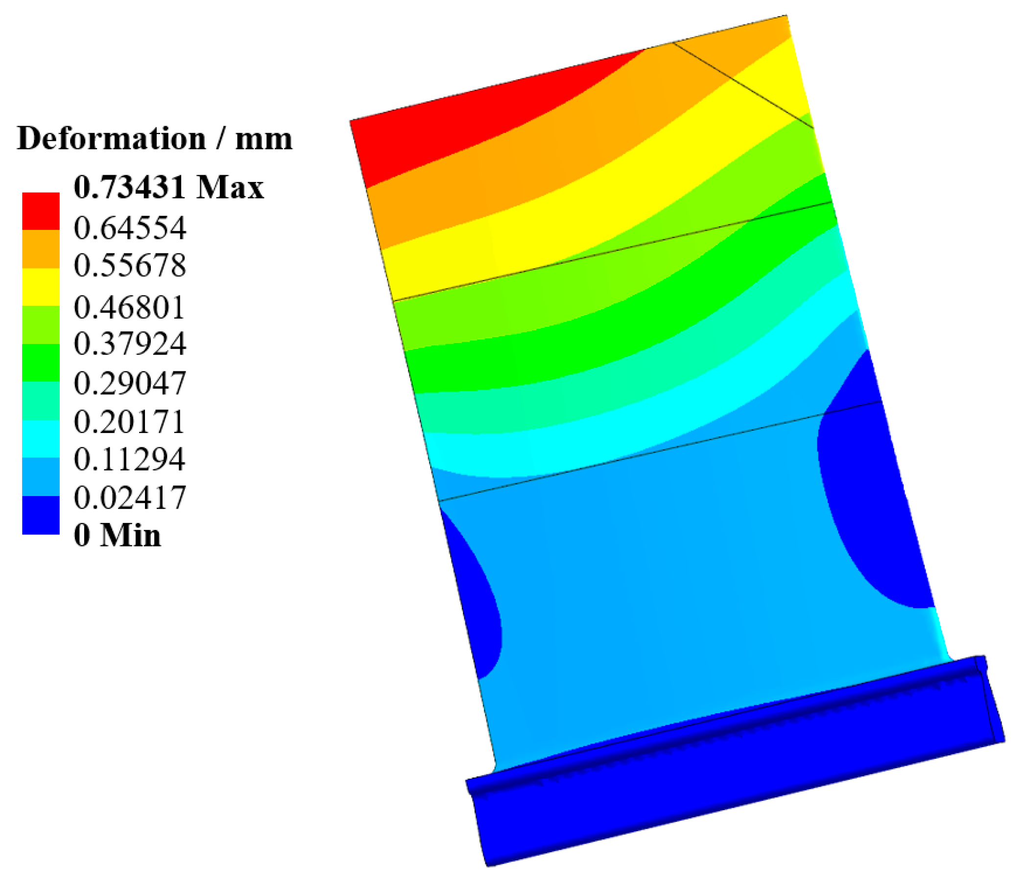
Figure 7.
Radial deformation distributions of compressor blade angle crack.
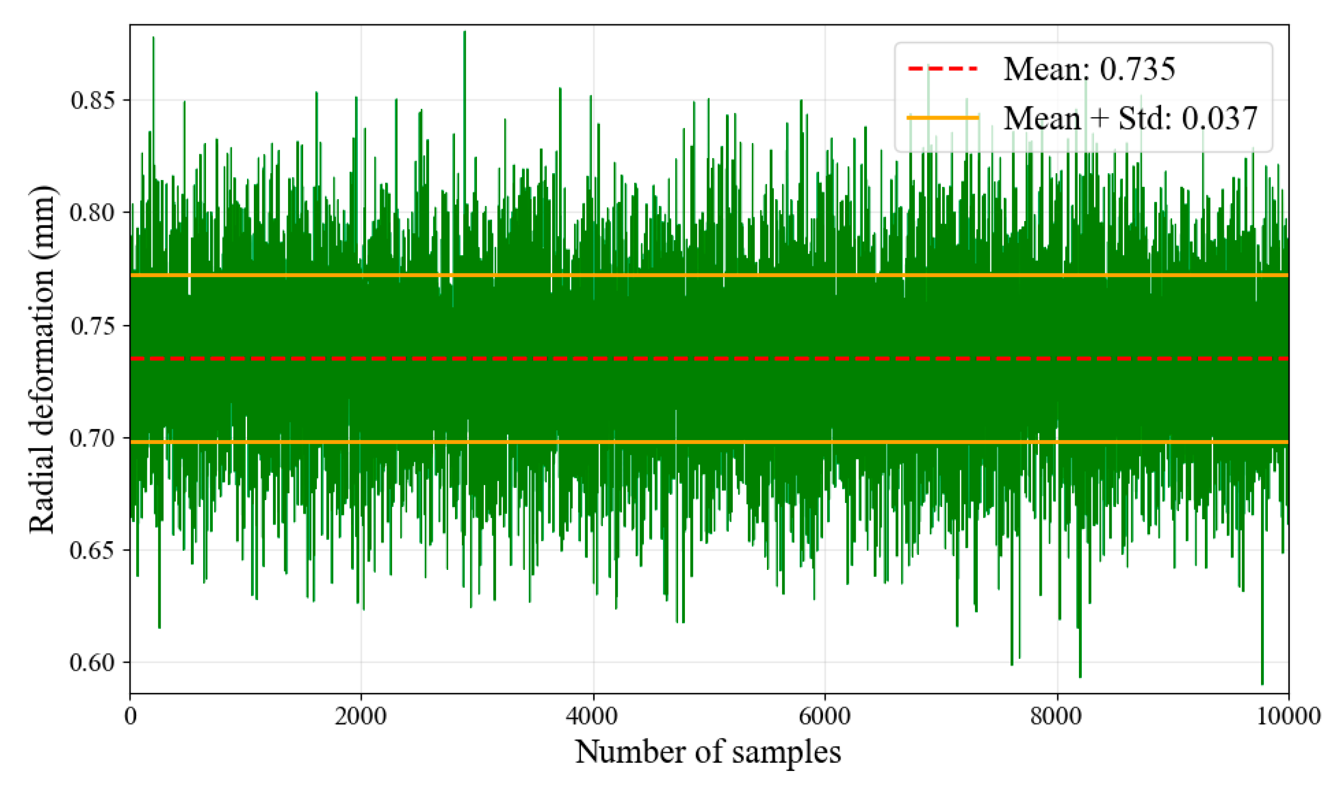
Figure 8.
Radial deformation probability density and cumulative distribution functions.
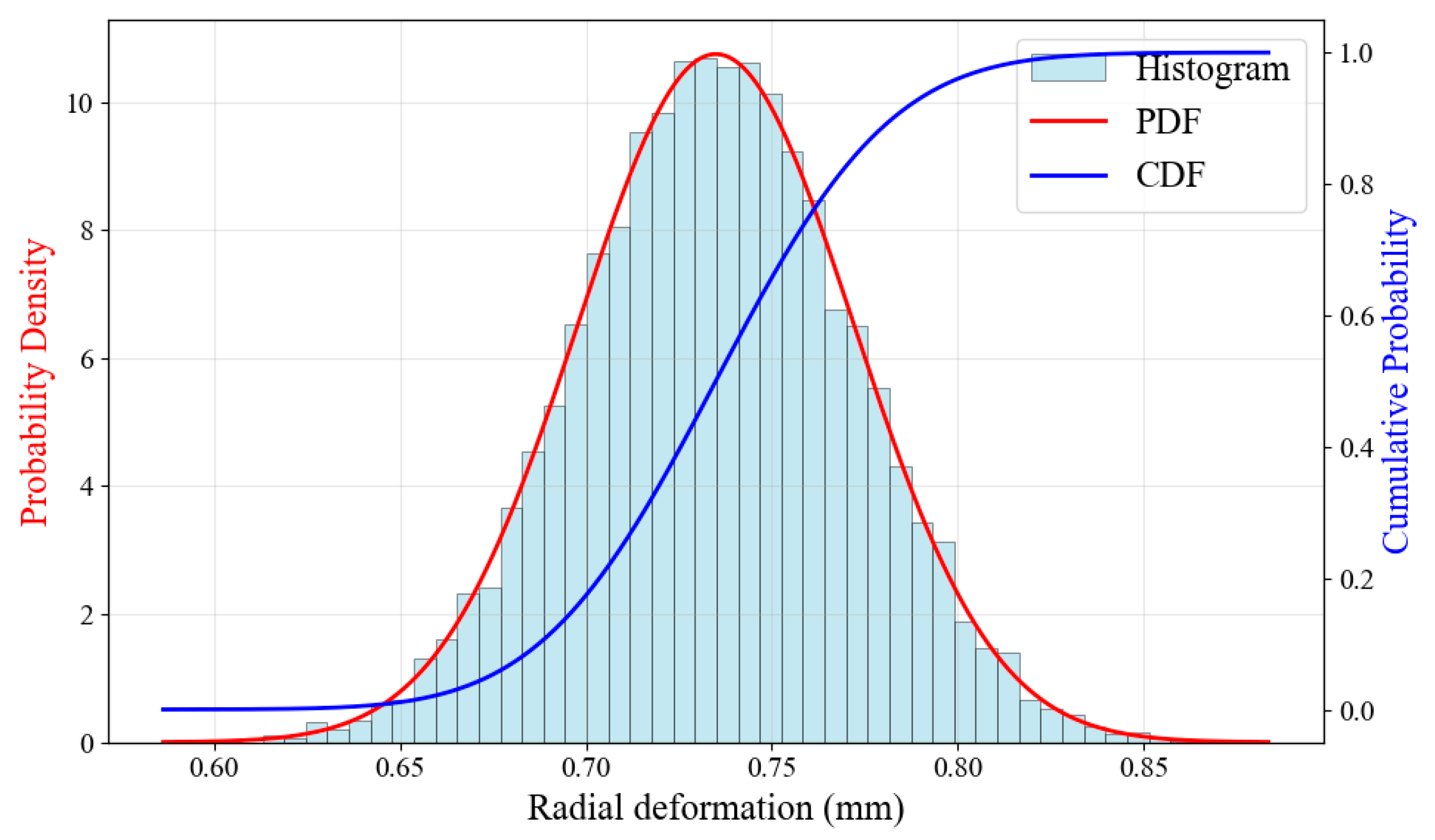
Figure 9.
Sensitivity index (dark bars) and importance index (light bars) for ten key input parameters.
Figure 9.
Sensitivity index (dark bars) and importance index (light bars) for ten key input parameters.
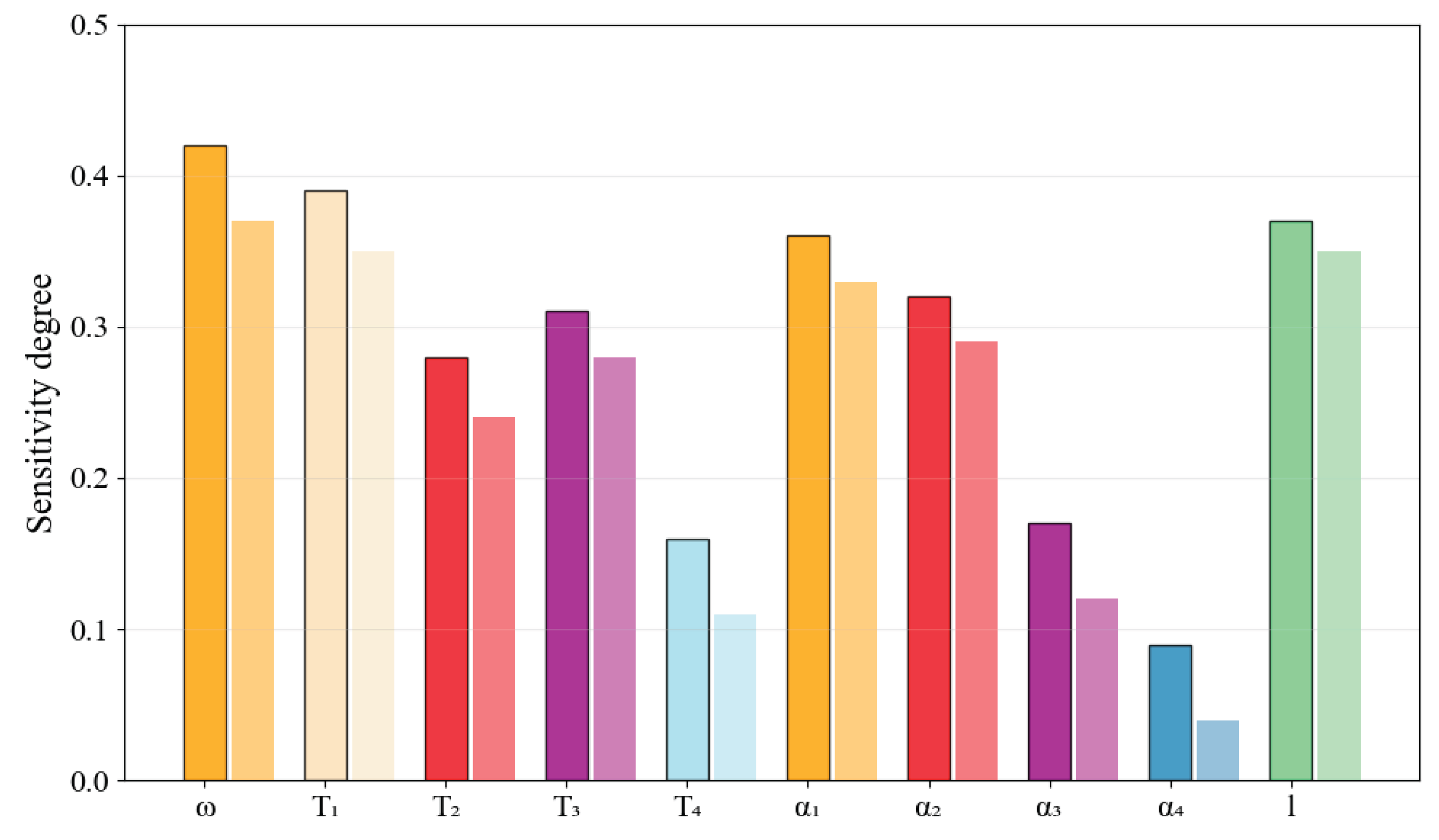

Table 1.
Statistical characteristics of uncertainty parameters.
| Parameter | Lower bound | Upper bound | Mean | Standard deviation | Distribution |
| ω(rad/s) | 101.5 | 194.5 | 148 | 15.51 | Normal |
| T1(℃) | 415.2 | 484.8 | 450 | 11.60 | Normal |
| T2(℃) | 291.1 | 408.9 | 350 | 19.65 | Normal |
| T3(℃) | 157.3 | 242.7 | 200 | 14.24 | Normal |
| T4(℃) | 25.2 | 74.8 | 50 | 8.27 | Normal |
| α1(Wm-2K-1) | 2259.6 | 2572.4 | 2416 | 52.13 | Normal |
| α2(Wm-2K-1) | 1873.7 | 2154.3 | 2014 | 46.78 | Normal |
| α3(Wm-2K-1) | 1432.2 | 1651.8 | 1542 | 36.61 | Normal |
| α4(Wm-2K-1) | 278.0 | 416.0 | 347 | 23.03 | Normal |
| l(mm) | 2.0 | 22.0 | 12.0 | 3.0 | Normal |
Table 2.
Degree of reliability for different MC samples.
| MCS | Degree of Reliability |
| 102 | 0.9512 |
| 103 | 0.9631 |
| 104 | 0.9712 |
| 105 | 0.9713 |
Table 3.
Parameter sensitivity indices and importance ranking.
| 1 | 2 | 3 | 4 | 5 | 6 | 7 | 8 | 9 | 10 | |
| S | 0.42 | 0.39 | 0.28 | 0.31 | 0.16 | 0.36 | 0.32 | 0.17 | 0.09 | 0.37 |
| I | 0.37 | 0.35 | 0.24 | 0.28 | 0.11 | 0.33 | 0.29 | 0.12 | 0.04 | 0.35 |
Table 4.
Performance comparison of different surrogate models.
| ModelType | RMSE | MAE | R2 | Training Time (s) | Prediction Time (s) |
| SVR | 0.847 | 0.623 | 0.7425 | 12.43 | 0.043 |
| ANN | 0.956 | 0.741 | 0.6723 | 45.67 | 0.013 |
| Kriging | 0.685 | 0.512 | 0.8313 | 8.94 | 0.024 |
| RBF | 0.737 | 0.548 | 0.8051 | 6.28 | 0.016 |
| GA-Kriging | 0.659 | 0.485 | 0.8445 | 78.72 | 0.031 |
| GA-RBF | 0.702 | 0.521 | 0.8234 | 69.41 | 0.026 |
| PSO-Kriging | 0.621 | 0.456 | 0.8616 | 88.31 | 0.028 |
| PSO-RBF | 0.675 | 0.498 | 0.8367 | 72.94 | 0.018 |
| OOA-KR (proposed) | 0.568 | 0.412 | 0.8842 | 52.82 | 0.025 |
Table 5.
Simulation precisions of reliability estimation for different methods.
| Simulation | 102 | 103 | 104 | |||
| Method | Reliability | Simulation Precision (%) | Reliability | Simulation Precision (%) | Reliability | Simulation Precision (%) |
| MCS | 0.99 | - | 0.999 | - | 0.9999 | - |
| SVR | 0.78 | 78.8 | 0.812 | 81.3 | 0.8241 | 82.4 |
| ANN | 0.69 | 69.7 | 0.731 | 73.2 | 0.7644 | 76.4 |
| Kriging | 0.84 | 84.8 | 0.866 | 86.7 | 0.8835 | 88.4 |
| RBF | 0.82 | 82.8 | 0.847 | 84.8 | 0.8672 | 86.7 |
| GA-Kriging | 0.86 | 86.9 | 0.881 | 88.2 | 0.8945 | 89.5 |
| GA-RBF | 0.83 | 83.8 | 0.856 | 85.7 | 0.8734 | 87.3 |
| PSO-Kriging | 0.87 | 87.9 | 0.892 | 89.3 | 0.9068 | 90.7 |
| PSO-RBF | 0.85 | 85.9 | 0.874 | 87.5 | 0.8891 | 88.9 |
| OOA-KR (proposed) | 0.91 | 91.9 | 0.962 | 96.3 | 0.9756 | 97.6 |
Disclaimer/Publisher’s Note: The statements, opinions and data contained in all publications are solely those of the individual author(s) and contributor(s) and not of MDPI and/or the editor(s). MDPI and/or the editor(s) disclaim responsibility for any injury to people or property resulting from any ideas, methods, instructions or products referred to in the content. |
© 2025 by the authors. Licensee MDPI, Basel, Switzerland. This article is an open access article distributed under the terms and conditions of the Creative Commons Attribution (CC BY) license (http://creativecommons.org/licenses/by/4.0/).
Copyright: This open access article is published under a Creative Commons CC BY 4.0 license, which permit the free download, distribution, and reuse, provided that the author and preprint are cited in any reuse.


