
Submitted:
06 August 2025
Posted:
08 August 2025
You are already at the latest version
Abstract
Rapid advancements in surveying technology have necessitated the development of more accurate and efficient tools. Leica Geosystems AG, a leading provider of measurement and surveying solutions, has initiated a study to enhance the capabilities of its GNSS INS-based surveying systems. This research focuses on integrating the Leica GS18I GNSS receiver and the AP20 AutoPole with a Time of Flight (ToF) camera through sensor fusion. The primary objective is to leverage the unique strengths of each device to improve accuracy, efficiency, and usability in challenging surveying environments. Results indicate that the AP20-ToF integration maintains decimeter-level accuracy and precision. Conversely, the GS18I-ToF integration exhibits decreased accuracy and requires further optimization. The fused AP20 configuration demonstrates superior efficiency and ease of use in challenging conditions compared to the GS18I setup. This analysis confirms the efficacy of the fused AP20 system, with deviations within acceptable limits for most practical applications, while highlighting the need for further refinement of the GS18I configuration.

Keywords:
Tilt Compensation
; Photogrammetry
; Real-Time Kinematic (RTK)
; Point Clouds
; Visual Positioning
; Geodesy
; Calibration
1. Introduction
An “imaging rover” is a special portable device with position and vision sensors to record and process visual data about an environment. In the surveying context, typically it is an integrated product of a GNSS (Global Navigation Satellite Systems) receiver with multiple cameras where, the GNSS receiver provides accurate positioning information from satellites and the cameras are incorporated to further enhance the accuracy, especially in GNSS-challenged areas [1]. In simple terms, the camera takes images of the environment, which can later be used to measure hard-to-reach points in that area. As GNSS faces problems in urban or indoor environments, an inertial measurement unit (IMU) is also used to complement GNSS in the rover by providing high-frequency motion data in the event of signal dropouts. Besides this, the IMU is capable of supplying the necessary orientation data to obtain a complete six-degree-of-freedom (6DoF) pose estimation, owing to its integrated accelerometer and gyroscope components [2]. This combination of GNSS with IMU is referred as an Inertial Navigation System (INS) [3]. Hence, imaging rovers provide a robust positioning solution for diverse surveying and mapping environments, from Unmanned Aerial Vehicles (UAVs) to ground surveying equipment [4]. For automotive and mobile mapping applications, this solution is versatile and is already being used in several studies [4,5,6] and the already available devices in the market, such as Trimble MX7 [7], RIEGL VZ-400i [8], ViDoc [9]: an add-on to a smartphone that has LiDAR, 3D Image vector [10], and Phantom 4 RTK [11], etc.
Although INS for mobile mapping applications is not new, this concept is developing critically for ground-based surveying since 2017. The concept was first proposed by Cera and Campi [12] and then by Baiocchi et al. [13]. Following this, Leica Geosystems AG introduced the GS18I, a GNSS sensor together with a built in 1.2 MP camera which enables visual positioning (allowing point measurement in captured images without pole straightening) [14]. Following Leica Geosystems AG, some other GNSS rovers offering visual positioning such as vRTK [15], INSIGHT V1 [16] and RS10 [17] also came to the market. In terms of survey grade accuracy, reliability and support, the GS18I by Leica Geosystems AG is by far the most commercially available and reliable surveying solution as confirmed by various performance studies [18,19]. However, when using the GS18I for image measurements, some conditions must be observed [19]. For example, the GS18I must receive sufficient GNSS signals throughout the measurement. If the GNSS satellite tracking is lost, the acquisition will automatically stop. If visual positioning is required, it should be avoided in darkness or when the camera is facing the sun, as not enough detail can be detected from the captured images to correlate them. In addition, the object needs to have a non-repetitive texture to allow the Structure from Motion (SFM) algorithm [20] to function properly. SFM is a photogrammetric technique that reconstructs three-dimensional structures from two-dimensional image sequences, relying on distinct visual features to estimate camera motion and object geometry. Alongside, for best results, images are captured from 2-10 m away. Distances less than 2 m may cause blurring due to fixed focus, while distances over 10 m reduce accuracy. Images taken outside this range may yield less precise measurements or may prevent point placement altogether.
In addition to complementing GNSS solutions, Leica Geosystems AG has introduced the AP20 AutoPole, the world’s first tilt able pole to complement total station workflows in 2022 [21]. Total stations excel in providing precise angle measurements, integrating angle and distance data in one device, and operating effectively where GNSS signals are unreliable or obstructed [22]. The AP20 automatically adjusts the inclination and height of the pole, eliminating the need to level the pole and separately record the height of the pole during surveying work. The AP20 also has integrated target identification (TargetID), which helps to ensure that the correct target is detected even if there are obstacles such as people or vehicles in the vicinity that could cause the total station to lose sight of the target. Currently, there are no direct equivalents from other manufacturers that offer the same combination of features specifically for Total Stations. However, the survey equipment industry is rapidly evolving and there is a need to further enhance the functioning and accuracy of these instruments.
For enhanced visual positioning and measurement accuracy, an idea could be to integrate a Time of Flight (ToF) camera in the GS18I and AP20. ToF cameras provide precise depth measurements by calculating the time it takes for light to travel to an object and back [23]. This depth information serves as the foundation for creating a 3D point cloud representation of a scene. ToF cameras can also work well in low light or even complete darkness since they provide their own illumination. The accuracy of ToF cameras exceeds any other depth detection technology, with the exception of structured light cameras, and can provide an accuracy of 1 mm to 1 cm depending on the operating range of the camera [24]. They are significantly more compact, speedy and have lower power consumption than other depth sensing technologies [24]. Combining real-time 3D data from a ToF camera with GNSS and tilt measurements could therefore address the challenges associated with GNSS limitations while extending the measurement range and improving visibility in low-light/dark conditions. It might also increase the operator’s safety and the measurement accuracy, especially for single point measurements without line of sight, or increase efficiency by speeding up data collection by reducing time spent in the field. This improved ease of use could also provide a competitive advantage over other products on the market.
For that matter, the primary aim of this work is to investigate the use of a ToF camera using the Leica GS18I and the AP20 as examples. In this regard, the Blaze 101 ToF camera from Basler AG was selected due to its performance data and potential suitability for outdoor surveying applications [25].
The structure of this case study is as follows: Section 2 covers a brief overview of the equipment and technologies used in this study. Section 3 presents the methodology for the integration process and the testing procedures to evaluate the performance of the integrated system. Section 4 sets forth the results and findings of the accuracy and performance tests, including specific metrics and comparative data in various use case examples. Section 5 reveals discussion about the challenges and solutions associated with this work and lastly, Section 6 summarizes the key outcomes of the case study and implications for future work.
2. Case Description: Materials and Technologies
In surveying, precision and efficiency are crucial. This case study explores a project that integrates a GNSS receiver (GS18I by Leica Geosystems AG), an intelligent surveying pole (AP20 by Leica Geosystems AG), and a ToF camera (Blaze 101 by Basler AG) to enhance GNSS-INS based surveying. From now on, we will refer to this integrated system as “Multi-Sensor-Pole (MSP)”. The integration of GS18I with the Blaze camera is termed the “GS18I-MSP”, while the integration of AP20 with the Blaze camera is called the “AP20-MSP” in the text. The following sections detail these specific instruments and the technologies used in them to achieve the project objectives.
2.1. Leica GS18I GNSS Receiver
The Leica GS18I is an advanced GNSS receiver designed for precise geodata and surveying tasks. It supports multiple satellite systems such as GPS, GLONASS, Galileo and BeiDou with 555 channels and multi-frequency capabilities. The device can update positions at a rate of up to 20 Hz, ensuring real-time data collection. It incorporates high-precision Real Time Kinematic (RTK) [26] with 8 mm + 1 ppm horizontal and 15 mm + 1 ppm vertical accuracy. The receiver works with the Leica Captivate software and offers various communication options such as Bluetooth, Wi-Fi, and USB as well as an optional UHF radio. It is equipped with a rugged, weatherproof design, an advanced GNSS antenna and a lithium-ion battery with up to 16 hours of operation.
The GS18I also incorporates an Inertial Measurement Unit (IMU) for tilt compensation, which does not require calibration and is immune to magnetic disturbances. This feature allows surveyors to measure hard-to-reach points without the need for precise levelling of the pole.
One of its standout features is the ability to perform visual positioning through its built-in camera via Structure from Motion (SfM) algorithms [20]. This allows for accurate point measurements from images, even in environments where direct GNSS measurements are challenging. The built-in camera is an Arducam AR0134 with 1.2 MP with a resolution of 1280 x 960 pixels (px) at a size of 3.75 µm and is equipped with a Bayer filter and a global shutter. The Field of View (FoV) of the camera is 80 degrees in horizontal and 60 degrees in vertical direction. The lens has a focal length of 3.1 mm, resulting in a ground scanning distance (GSD) of 12 mm at 10 meters [14]. A quick depiction of GS18I is shown in Figure 1.
The orientation of GS18I is measured at 200 Hz by its integrated INS [27]. This orientation is important in estimating the position and orientation (pose) of the built-in camera images in a global coordinate system. The INS also generates a synchronization pulse that triggers both the built-in camera and the external Blaze ToF camera, ensuring temporal alignment of image acquisition across both sensors in the GS18I-MSP setup. The details of this trigger process will follow in Section 3.4.
2.2. Leica AP20 AutoPole
The AP20 is a high-tech version of a surveying pole that provides a vertical reference point for measurements (Figure 2). A prism is attached to the top of the AP20, which reflects the laser beam emitted by a total station towards it. The total station uses reflected laser signals not only to measure the distance between the AP20 and itself, but also to detect and continuously track the prism using Leica’s ATRplus (automatic target recognition and tracking technology) as the surveyor moves the pole around the site. Unlike traditional survey poles, the AP20 automates several tasks that traditionally require manual input, thereby increasing efficiency and reducing errors. For instance, its tilt compensation allows surveyors to measure points at any angle up to 180° without needing to level the pole. This capability is especially useful for measuring hard-to-reach points, such as building corners or objects under obstacles [21]. The AP20 also includes automatic pole height measurement, eliminating the need for manual height adjustments. The device operates in a wide temperature range from -20°C to +50°C and is protected against dust and water with an IP66 rating. Technologically, the AP20 uses an Inertial Measurement Unit (IMU) for precise tilt measurements and Bluetooth/radio frequency for wireless connectivity [21].
It is worthwhile to mention here that a special AP20 from Leica Geosystems AG was provided for this case study. In contrast to the standard AP20, this special AP20 had the feature to supply the device over the integrated USB-C connector and reading IMU and TPS data directly from the onboard ROS-Publisher over the USB 2 interface. ROS (Robot Operating System) is an open-source software framework that provides a set of tools, libraries, and conventions for developing complex robotic systems and facilitating communication between different software components [28]. More details are provided in Section 3.2. Similarly to GS18I, the built-in IMU of AP20 also generates a trigger pulse, which triggers the Blaze ToF camera in the AP20-MSP setup; see Section 3.4.
2.3. Basler Blaze 101 ToF Camera
The Basler Blaze 101 is a Time-of-Flight camera that provides high-precision depth sensing and 3D imaging [25]. It features a resolution of 640 x 480 pixels and can capture up to 30 frames per second, delivering detailed depth information with an accuracy of ±5 mm within a range of 0.3-5.5 m. The operating wavelength is 940 nm. Besides, the camera has an effective measurement range of 0-10 m. However, due to the nature of ToF technology, there is an ambiguity issue where objects beyond 10 m may be detected as being closer (e.g., an object at 24 m might be detected as 4 m away). The Blaze 101 supports multiple output formats, including depth map, intensity image, and point cloud data. It comes with an SDK (Software Development Kit) for Windows and Linux, and provides interfaces such as Gigabit Ethernet and digital I/O. The camera’s compact size of 100 x 65 x 60 mm and its IP67 housing make it suitable for industrial environments. Additionally, it offers features like multi-camera operation and HDR mode for challenging lighting conditions (Figure 3).
The Blaze 102 ToF camera is another variant of the ToF cameras from Basler AG [29]. This camera shares many similarities with the Blaze 101, including resolution, frame rate, interface, working range, and the ability to generate 2D and 3D data simultaneously. However, the key difference is that Blaze 102 operates at 850 nm, while the Blaze 101 uses 940 nm. The Blaze 101 offers superior immunity to ambient light compared to the Blaze 102 camera. For this case study, the behaviour of both cameras was tested by conducting various tests particularly focusing on accuracy, distance, and environmental factors. To check for interference, two Blaze 101 and 102 cameras were also used together. The details of these tests are not discussed here as they would go beyond the scope of this paper. However, it turned out that the Blaze 101 is not only more suitable for outdoor use in bright sunlight, but also performs comparable to Blaze 102 indoors or in cloudy conditions. Besides, using two Blaze 101 cameras instead of one slightly increased the FoV but also caused interference. Besides, saving data with two cameras required a more computer processing power and storage. Therefore, for the rest of this study, only Blaze 101 was used for the MSP testing.
3. Methodology
This section first presents a functional measurement setup of the Multi-Sensor-Pole. Then the relevant steps to assemble the components used in the functional model are described. Later, details about data processing and analysis are explained.
3.1. Functional Model
The functional setup of the Multi-Sensor-Pole is shown in Figure 4 where the two Blaze 101 cameras are mounted inside a steel bracket on a vertical pole. The pole provided stability and allowed the setup to be positioned at a desired height. The topmost device could be the GS18I or AP20. A laptop and the CS30 control unit for the GS18I are also attached to the pole below the steel bracket for real-time data acquisition, monitoring, and control of the sensors’ behaviour. The laptop is connected to the sensors via cables, which are explained in the next Section 3.2.
3.2. I/O Connections for Powering and Triggering
The GS18I was powered by an internal battery (GEB333). The Blaze cameras came with a 24V / 60W power supply and an adjustable M12, M, 8-Pin / Open I/O cable from Basler AG. This cable has an 8 pin open ended connector that can be customised for powering the cameras and to allow an external trigger operation. Accordingly, Leica Geosystems AG provided two custom-made cables for powering and triggering the Blaze camera via the GS18I and AP20. An overview of these connections is given in Figure 5 for the connection with GS18I and in Figure 6 for the connection with AP20.
A detailed description for the Blaze connector’s pin numbering and assignments can be found at [25]. For data collection, a separate GigE M12, M, 8-pin/RJ45 data cable was also purchased from Basler AG.
3.3. Frame Grabber and the Portable Computer
The pylon Camera Software Suite allows all the necessary tools for easy integration and set-up of the Blaze ToF cameras through a single interface. The software is available for Windows, ARM-based, and AMD-based Linux systems. The “Blaze Viewer” and “pylon IP Configurator” that come in the pylon Camera Software Suite allow for setting up the triggering and configuring parameters of Blaze cameras through software. The “Blaze Viewer” can be then used as a Frame Grabber from Blaze ToF sensors. However, for this case study, the data were collected and stored in ROS bags [30]. A laptop (HP ZBook 15 G5 Intel i7 8850H 2.60GHz 32GB RAM 500GB Linux) was used for continuous image buffering and acquisition from the Blaze camera.
3.4. Trigger Operation
Blaze camera can be triggered externally by an external triggering source at pin 6 (Line0) by using a trigger signal having a range of 0-24V. The trigger is always a FrameTrigger, i.e., it triggers the acquisition of a single frame in the current operating mode.
Both GS18I and AP20 were used as an external trigger source for the Blaze camera using specially designed trigger cables as shown in Figure 5 and Figure 6. The INS of the GS18I can provide a trigger signal of ±5 V from Pin 8 of its Port P1, which is enough to meet the Blaze camera specification for trigger. The emission of the trigger pulse from the GS18I to the Blaze cameras must be activated via the GeoCOM command. The GeoCOM command interface is a specially designed communication protocol used by Leica total stations and GNSS receivers to enable interaction with non-Leica software packages and external devices [31]. These commands can be used to configure the GS18I for starting and stopping the trigger and for the image acquisition rate by the Blaze. For the GS18-MSP, the frame rate was set to 10 Hz, to avoid rapid memory filling, as the GS18I can currently only store image data on its SD card for one minute.
For sending the trigger pulse from the AP20, specially designed AP20 Firmware was used, which generated a hardware trigger signal synchronized with the AP20 onboard IMU to trigger the frames of the Blaze. For this setup, the frame rate was set to 20 Hz, as it was currently not possible to reduce the frame rate of the IMU of the AP20. For optimal performance, the total station was placed at a distance of at least 5 metres from the AP20 prism to obtain best position data.
3.5. Calibration
Camera calibration is the process of determining and adjusting a camera’s internal (intrinsic) and external (extrinsic) parameters to ensure accurate and distortion-free image capture. Generally, intrinsic parameters involve estimating the focal length of the camera in width and height, the optical centre, and the distortion coefficients, which quantitatively indicate lens distortion. On the other hand, the extrinsic parameters represent the camera’s position in the 3D scene: the rotation and translation. Combining these parameters in a camera Projection matrix (P) provides the necessary calibration of the camera.
For MSP configurations, the extrinsic calibration process was achieved using the Kalibr Toolbox [32]. This tool supports the “Multiple camera calibration”, which was required for calibrating the GS18I’s camera with the Blaze camera in the GS18I-MSP, based on the algorithm defined in [33]. Similarly, Kalibr also has a “Camera IMU calibration” tool defined in [34], which was required to calibrate the Blaze ToF camera with the IMU of AP20 in the AP20-MSP.
The MSP calibration process was carried out in accordance with the guidelines mentioned at the Kalibr website [32]. For using the “Multiple camera calibration” tool in Kalibr, the image data was provided as a ROS bag containing the image streams from the Blaze and the GS18I. To capture the image data, the Aprilgrid Target provided by Kalibr (see Figure 7) was glued to a rigid board and moved around the GS18I-MSP setup. For image synchronization, the Blaze camera was triggered by the GS18I as explained in Section 3.4. The intensity images captured from the Blaze camera were captured in 8-bit .PNG format while the images from the GS18I were in .JPG format. By using the“bagcreator” script provided in Kalibr, a ROS-version 1 bag was created on the sequence of acquired images. This bag was then used to run the Kalibr calibration commands, which in turn returned the camera Projection matrix with reference to the GS18I and the Blaze separately.
Similarly, for using the “Camera IMU calibration” tool, a ROS-version 1 bag was also recorded directly containing the IMU data from the AP20 and the intensity images from the Blaze. In this case, the calibration target (Figure 7) was fixed and the AP20-MSP setup was moved in front of the target to excite all IMU axes of the AP20. The output of running Kalibr commands on the recorded ROS bag gave the necessary transformation matrices (from IMU frame to the camera frame) and the time shift parameter indicating the temporal offset between the Blaze camera and the IMU of the AP20.
3.6. Data Collection and Storage
For the GS18I-MSP, the image and pose data from the GS18I were stored directly on the sd-card mounted inside it, while the images/point clouds from the Blaze were recorded in a ROS bag. To perform live measurements, live pose of the GS18I can also be stored in ROS bag along with the Blaze.
For the AP20-MSP, data from the AP20 and the Blaze camera were captured and recorded in ROS bags. These ROS bags can replay the recorded data easily using the built-in ROS visualization tools like “rviz” and “rqt_bag” [30].
3.7. Test Areas and the Measurements Setup
The AP20-MSP was tested both indoors and outdoors, while the GS18I-MSP was only tested outdoors since the GS18I loses satellite reception inside. For indoor live testing of AP20-MSP, the measurement laboratory of the Institute Geomatics, University of Applied Sciences and Arts Northwestern Switzerland was used; see Figure 8.
For outside testing, one of the houses situated at Arlesheim, Switzerland was used as shown in Figure 9. The front part of the house faces the road, while the rear part is shaded by tall trees in the backyard. The idea behind choosing this location was to have a real-life survey scenario where some points are directly accessible, while the others are either not in the direct line of sight or in areas with GNSS problems, or in areas where the surveyor can see them but cannot reach them. It was also necessary to test whether the range of the survey area could be extended with the MSP setups with sufficient GNSS/total station reception.
4. Results
Live single point measurement was tested using the AP20-MSP in a lab environment (Figure 8), with six checkerboard targets attached to the wall. The Leica MS60 Multi-Station provided reference measurements. Despite reasonable accuracy and precision at shorter distances (150-350 cm), the experiment revealed a time-synchronization issue between the pose integration and point clouds. This issue prevented reliable live single point measurements, particularly at longer distances.
For outdoor testing with both setups, three targets were fixed on tripods at three different locations around the house: one at the front, one in the middle and one at the back courtyard of the house (Figure 9). The whole area was scanned with the 3D laser scanner (RTC360) from Leica Geosystems AG. The RTC360 can capture up to 2 million points per second. The scan obtained from the RTC360 is shown in Figure 10 and was used as a reference point cloud to compare the measurements later.
The corresponding synchronized point cloud taken by the AP20-MSP with a blue-white-red gradient scale is shown in Figure 11(a) and the point cloud taken from the GS18I-MSP is shown in Figure 11(b). The blue-white-red gradient when applied to a point cloud typically represents a visual encoding of distance or scalar field values when compared to another cloud. For example, in Figure 11, the blue points are in or near the reference RTC360 cloud (e.g., 0 cm). Points that are approximately 10 cm from the reference cloud are coloured white, while points coloured red are at or near 20 cm from the reference point. Then the points away from 20 cm are shown in grey. Note that the point cloud from the GS18I-MSP is quite grey, which means that these points are more than 20 cm away from the reference cloud. The different patches blend worse than the ones from the AP20. This is probably a consequence of the different accuracy of the poses.
With each MSP, multiple sets of data were recorded around the house. Three sets of measurements were taken with the AP20-MSP while nine sets were taken with the GS18I-MSP with the following reference points:
- Measured with Leica MS60: Points labelled as hp1, hp2, and hp3 were measured using the Leica MS60. The setup point of MS60 was calculated with a resection using three LFP3 points in the region and one HFP3 for height (LFP3 and HFP3 are official survey points in Switzerland that are managed by the municipality or a contractor of the municipality). The standard deviation for easting and northing was 1.2 cm.
- Natural Points: Points labelled b1 and w1 were measured in the reference point cloud, geo-referenced with laser scanning targets on tripods. A height offset of 6.5 cm exists from the round prism to the laser scanning target. The geo-referencing process had a final RMS of 1.2 cm.
- Measured with GS18: Points labelled hp10, hp11, and hp12 were measured with the GS18I on a different day due to some technical difficulties, necessitating a second measurement campaign. To align this one with the other measurements, the laser-scanning targets were removed and the points were measured with the GS18. The 3D-Accuracy was below 5 cm for all measurements.
The accuracy expectations for the Multi-Sensor-Pole configurations vary based on the reference points and measurement methods. For the AP20-MSP, measurements taken with the MS60 are expected to have an accuracy combining the AP20’s inherent accuracy with a 1.2 cm standard deviation, with measurements closely matching the total station positions. The Reference Cloud 1 calculations for AP20 follow a similar pattern.
In fact, the measurements from the Blaze camera are noisier than those from the RTC360. It might also depend on how fast the Multi-Sensor-Poles were moving during the collection of the point clouds. However, synchronization with poses from GS18I should be nearly perfect due to the matching of GS18I images and intensity images from the Blaze camera. Likewise, the measurements of AP20 are nearly exactly a multiple of 10 of the Blaze Images (since the IMU rate of AP20 is 200 Hz and positioning updates were coming at 20 hz measuring rate from the MS60). However, drag effects might have occurred when updating the 6-DOF pose. A comparison of a point cloud taken from RTC360, AP20-MSP, and GS18I-MSP of a Laser scanning Target from the best sets is shown in Figure 12.
From the best datasets, some measurements were taken for comparison. Since the GeoCom command used in the GS18I-MSP gave the measurement coordinates in the ECEF (Earth-Centred, Earth-Fixed) reference system, these values were first transformed into WGS84 coordinates with the Pymap3d library of the Python programming language. The WGS84 coordinates were then transformed into the Swiss Coordinate System (LV95). Among these measurements, the relative and absolute distances from both MSP setups have been calculated and shown in Section 4.1 and Section 4.2. The relative distances are the distances calculated inside the point clouds, while the differences to the geo-referenced coordinates have been calculated as absolute distances.
4.1. Relative Distances
The differences in relative distances within the point clouds for the AP20-MSP are minimal as shown in Table 1. For example, the distance between reference points hp1 and hp3 is only off by 1.21 cm, and the largest deviation observed is 15.34 cm (hp1-b1) This suggests that the AP20-MSP maintains good internal consistency and accuracy relative to the reference measurements. The relatively consistent and small errors across different point pairs also suggest good precision.
The GS18I-MSP showed larger deviations in relative distances, with some differences exceeding 20 cm (see Table 2). The largest observed deviation was 21.3 cm for hp12-w1. This suggests that the internal consistency of the GS18I-MSP measurements is less reliable compared to the AP20-MSP.
4.2. Absolute Distances
For AP20-MSP, when comparing absolute distances, hp1 showed a 3D error of 2.69 cm and b1 had a more substantial error of 15.95 cm. However, the absolute errors for the AP20-MSP are within 3 cm for signalized points, such as hp1 and hp3, indicating that accuracy on the decimetre level is achievable (Table 3).
With the GS18I-MSP, the absolute distance errors were notably larger: w1 had a 3D error of 25 cm, while hp13, which is significantly better, still had a error of 8 cm (see Table 4).
Although the Multi-Sensor-Pole used in this conceptual study is not yet a ready-to-use device, the results clearly demonstrate that integrating a ToF camera with GNSS and IMU technologies in the system can enhance surveying capabilities, allowing measurements in low-light or hard-to-reach areas without direct contact or line of sight. This is particularly valuable for challenging environments like steep slopes or hazardous locations, allowing surveyors to work from a safe distance. The Multi-Sensor-Pole could also improve stake-out operations by offering precise visual guidance, potentially with augmented reality features to overlay digital information, reducing errors and saving time. Additionally, it enables the creation of more accurate 3D models, benefiting applications such as Building Information Modelling, infrastructure inspection, and topographic mapping. In summary, the key benefits of using a Multi-Sensor-Pole include:
- Improved low-light performance for night-time or indoor surveying.
- Enhanced accuracy, minimizing the need for multiple setups.
- Simultaneous capture of positional and visual data for greater efficiency.
- Versatility across diverse surveying and mapping applications.
5. Conclusions
The analysis of the AP20-MSP and GS18I-MSP configurations reveals significant differences in their performance. The AP20-MSP demonstrates superior accuracy and precision, achieving decimeter-level measurements with absolute errors within 3 cm for signalized points. This configuration maintains high internal consistency and effectively synchronizes with the Basler Blaze 101 ToF camera, making it suitable for high-precision surveying tasks. In contrast, the GS18I-MSP configuration exhibits larger errors, often exceeding 20 centimeters, and shows inconsistencies between measurement sets, indicating a need for optimization in pose estimation and transformation processes. With regard to efficiency, the AP20-MSP proves to be more effective for various surveying use cases, particularly in challenging environments. It is well suited for applications that require precise measurements, such as construction surveys, topographic mapping, and infrastructure monitoring. The GS18I-MSP, while functional, requires further optimization to improve its accuracy and efficiency, limiting its current applicability in high-precision tasks but potentially useful in scenarios where rapid data collection is prioritized over extreme accuracy.
Author Contributions
Conceptualization, Joël. B. and David. E.G.; methodology, Joël. B. and Amna. Q.; software, Amna. Q; validation, Joël. B.; formal analysis, Joël. B.; investigation, Amna. Q. and Joël. B.; data curation, Amna. Q. and Joël. B.; writing—original draft preparation, Amna. Q.; writing—review and editing, David. E.G.; supervision, David. E.G.; project administration, Amna. Q. and David. E.G.; funding acquisition, David. E.G. All authors have read and agreed to the published version of the manuscript.
Funding
This research was funded by Leica Geosystems AG grant number.
Institutional Review Board Statement
The study was approved by the Leica Geosystems AG.
Data Availability Statement
The original contributions presented in this study are included in the article/supplementary material.
Conflicts of Interest
The authors declare no conflicts of interest. The funders had no role in the design of the study; in the collection, analyses, or interpretation of data; in the writing of the manuscript. However, the funders had role in making the decision to publish the results.
References
- Introduction to GNSS IMU Systems, 2023.
- Angelino, C.V.; Baraniello, V.; Cicala, L. UAV position and attitude estimation using IMU, GNSS and camera; 2012. Journal Abbreviation: 15th International Conference on Information Fusion, FUSION 2012 Publication Title: 15th International Conference on Information Fusion, FUSION 2012. [Google Scholar]
- Inertial navigation system, 2024. Page Version ID: 1232418048.
- Chu, T.; Guo, N.; Backén, S.; Akos, D. Monocular Camera/IMU/GNSS Integration for Ground Vehicle Navigation in Challenging GNSS Environments. Sensors 2012, 12, 3162–3185. [Google Scholar] [CrossRef] [PubMed]
- Multisensor Navigation Systems: A Remedy for GNSS Vulnerabilities? | IEEE Journals & Magazine | IEEE Xplore.
- Li, T.; Zhang, H.; Gao, Z.; Niu, X.; El-sheimy, N. Tight Fusion of a Monocular Camera, MEMS-IMU, and Single-Frequency Multi-GNSS RTK for Precise Navigation in GNSS-Challenged Environments. Remote Sensing 2019, 11, 610. [Google Scholar] [CrossRef]
- Inc, T. Trimble MX7 | Mobile Mapping Systems, 2024.
- Laser Measurement Systems, R. RIEGL - Produktdetail, 2024.
- viDoc: GNSS multi-measurement tool.
- 3dimagevector - REDcatch GmbH, 2021.
- Enterprise, D. Phantom 4 RTK, 2024.
- Cera, V.; Campi, M. Evaluating the potential of imaging rover for automatic point cloud generation. The International Archives of the Photogrammetry, Remote Sensing and Spatial Information Sciences, W3. [CrossRef]
- Baiocchi, V.; Piccaro, C.; Allegra, M.; Giammarresi, V.; Vatore, F. Imaging rover technology: characteristics, possibilities and possible improvements. Journal of Physics: Conference Series 2018, 1110, 012008. [Google Scholar] [CrossRef]
- Geosytems, L. GS18 I – Leica Geosystems Surveying, 2018.
- Land Survey – New Pocket-Sized vRTK is the Perfect Combination of GNSS, Advanced IMU, and Dual Cameras, 2022.
- Mapping Technology, S.S. INSIGHT V1.
- Navigation, C. CHCNAV Unveils RS10: A revolutionary integrated handheld SLAM laser scanner with GNSS RTK system, 2024.
- Casella, V.; Franzini, M.; Manzino, A. GNSS and photogrammetry by the same tool: a first evaluation of the leica gs18i receiver. The International Archives of the Photogrammetry, Remote Sensing and Spatial Information Sciences, 2021. [Google Scholar] [CrossRef]
- Păunescu, C.; Potsiou, C.; Cioacă, A.; Apostolopoulos, K.; Nache, F. Introducing New Technology in the cadastral surveying. Technical Report 1 1137, Netherlands, 2021. [Google Scholar]
- Lobo, T. Understanding Structure From Motion Algorithms, 2023.
- Oudtshoon, A.v. The next evolution: introducing the new Leica AP20 AutoPole!, 2022.
- Faro, M. Advantages of using Total Stations over GNSS in surveying | LinkedIn, 2023.
- Kumar, P. What is a ToF sensor? What are the key components of a ToF camera?, 2021.
- What are Depth-Sensing Cameras and How do They Work?, 2024.
- blaze-101 | Basler, AG.
- Teunissen, P.J.G.; Khodabandeh, A. Review and principles of PPP-RTK methods. Journal of Geodesy 2015, 89, 217–240. [Google Scholar] [CrossRef]
- Studemann, G.L. Higher Resolution Camera for an Imaging Rover and Low-Cost GNSS Setup for Water Equivalent of Snow Cover Determination. Masterthesis, FHNW, Muttenz, 2022.
- ROS/Tutorials/UnderstandingNodes - ROS Wiki.
- blaze-102 | Basler, AG.
- Bags - ROS Wiki.
- GeoSystems, L. TPS-1200 GeoCOM Reference Manual, Version 1. 20. 2005. [Google Scholar]
- ethz-asl/kalibr, 2024. original-date: 2014-05-29T12:31:48Z.
- Maye, J.; Furgale, P.; Siegwart, R. Self-supervised calibration for robotic systems. In Proceedings of the 2013 IEEE Intelligent Vehicles Symposium (IV); 2013; pp. 473–0587. [Google Scholar] [CrossRef]
- Unified temporal and spatial calibration for multi-sensor systems | IEEE Conference Publication | IEEE Xplore.
Figure 1.
Leica GS18I: (a) top view. (b) front view with the built-in camera. (c) side view showing the battery compartment and the services panel. (Source: [14])
Figure 1.
Leica GS18I: (a) top view. (b) front view with the built-in camera. (c) side view showing the battery compartment and the services panel. (Source: [14])
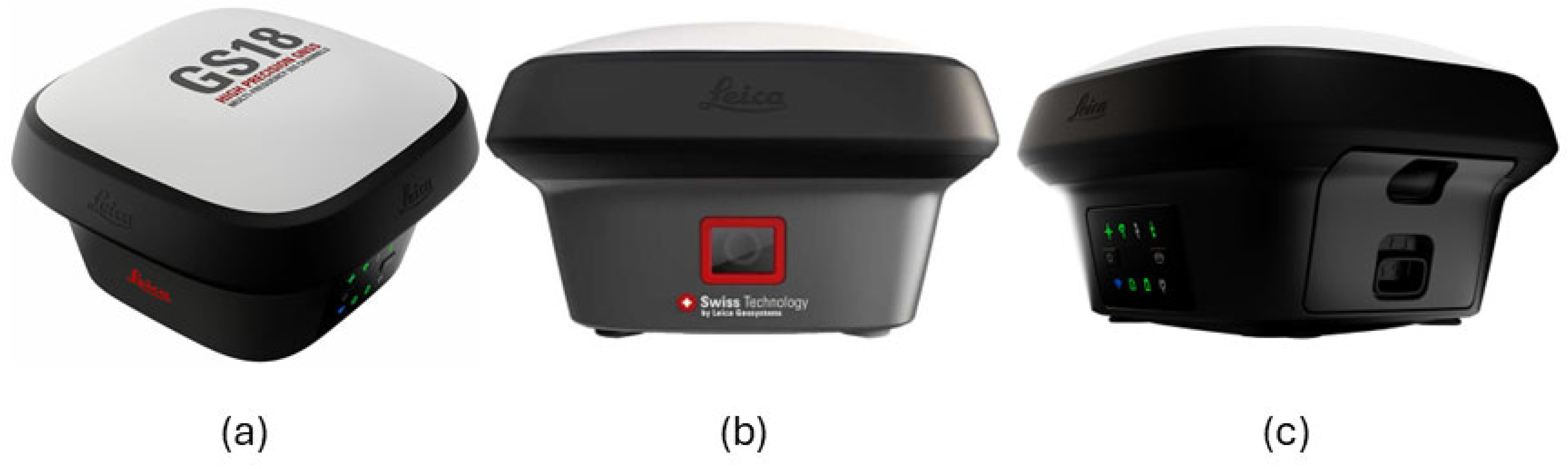
Figure 2.
Leica AP20 AutoPole with Leica GRZ4 360° prism attached. (Source: [21])
Figure 2.
Leica AP20 AutoPole with Leica GRZ4 360° prism attached. (Source: [21])
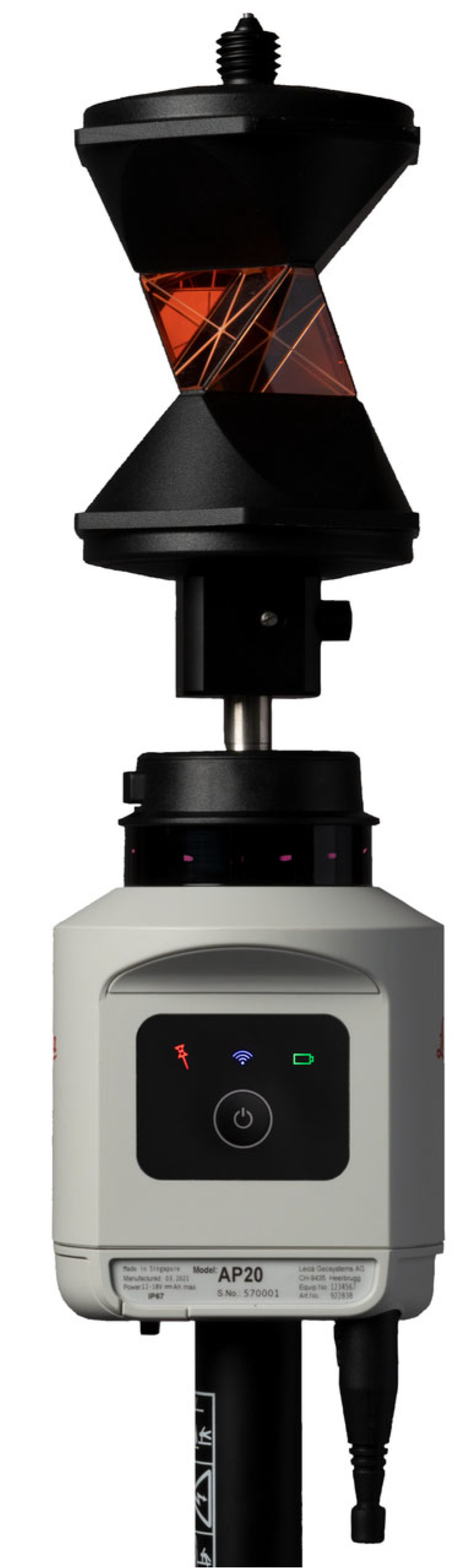
Figure 3.
Basler Blaze 101 Time of Flight camera with front and back views. (Source: [25])
Figure 3.
Basler Blaze 101 Time of Flight camera with front and back views. (Source: [25])
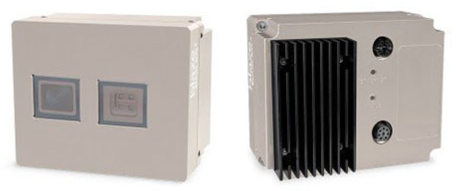
Figure 4.
The functional model of Multi-Sensor-Pole with GS18I (a) and AP20 (b). The prism used is the Leica MRP122.
Figure 4.
The functional model of Multi-Sensor-Pole with GS18I (a) and AP20 (b). The prism used is the Leica MRP122.
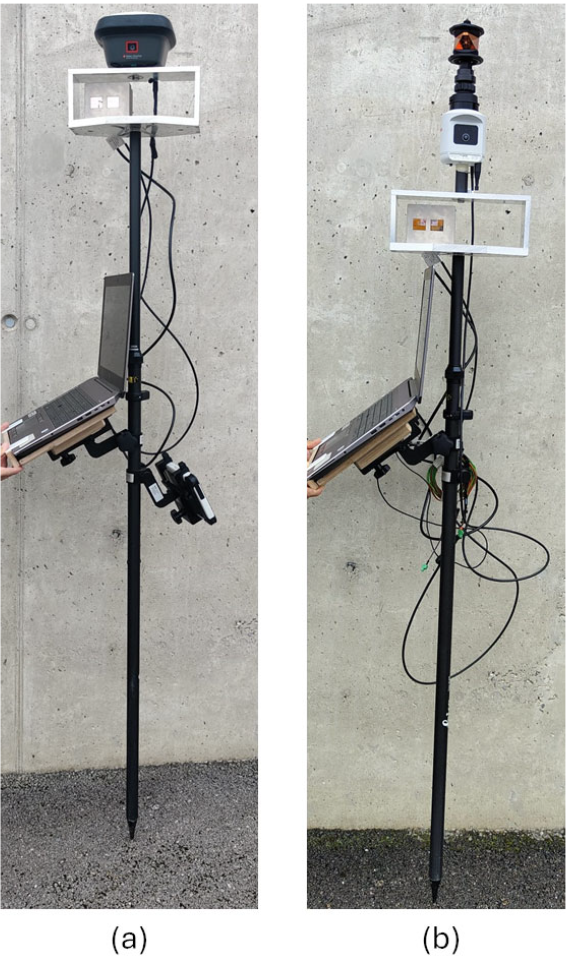
Figure 5.
The customised I/O cables provided by Leica Geosystems AG to trigger Blaze cameras by the GS18I.
Figure 5.
The customised I/O cables provided by Leica Geosystems AG to trigger Blaze cameras by the GS18I.
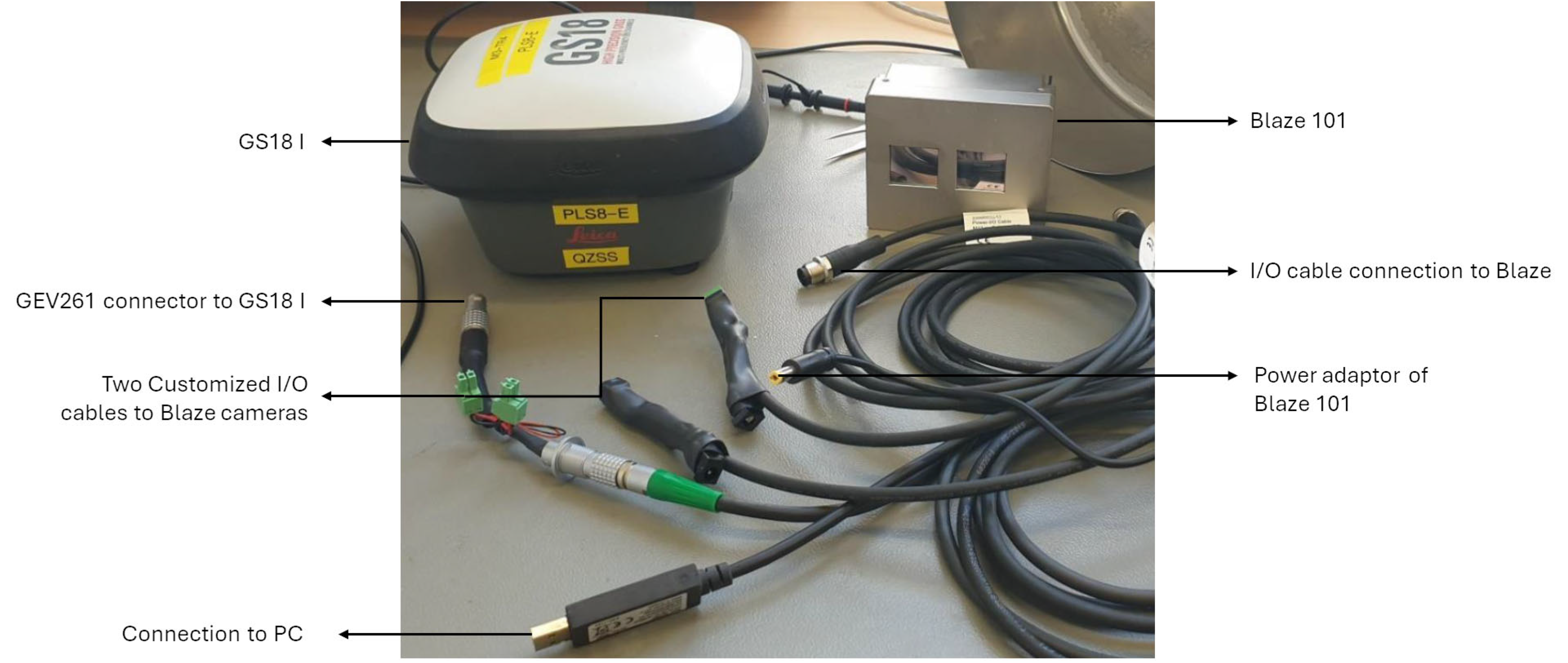
Figure 6.
The AP20 can be powered over a USB-C connector besides providing the trigger to the Blaze camera through the customized I/O cable provided by Leica Geosystems AG.
Figure 6.
The AP20 can be powered over a USB-C connector besides providing the trigger to the Blaze camera through the customized I/O cable provided by Leica Geosystems AG.
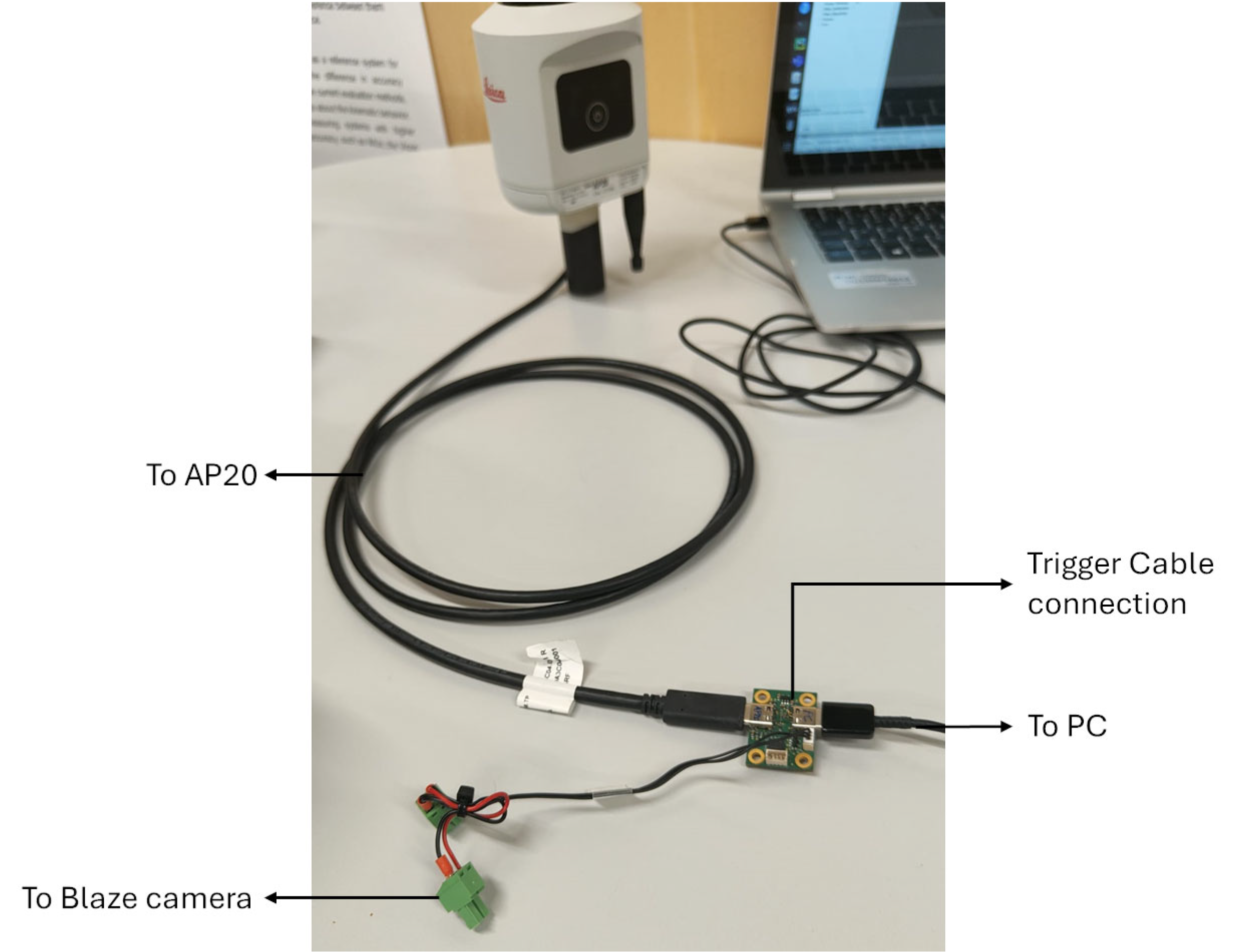
Figure 7.
The Aprilgrid target used for the calibration.
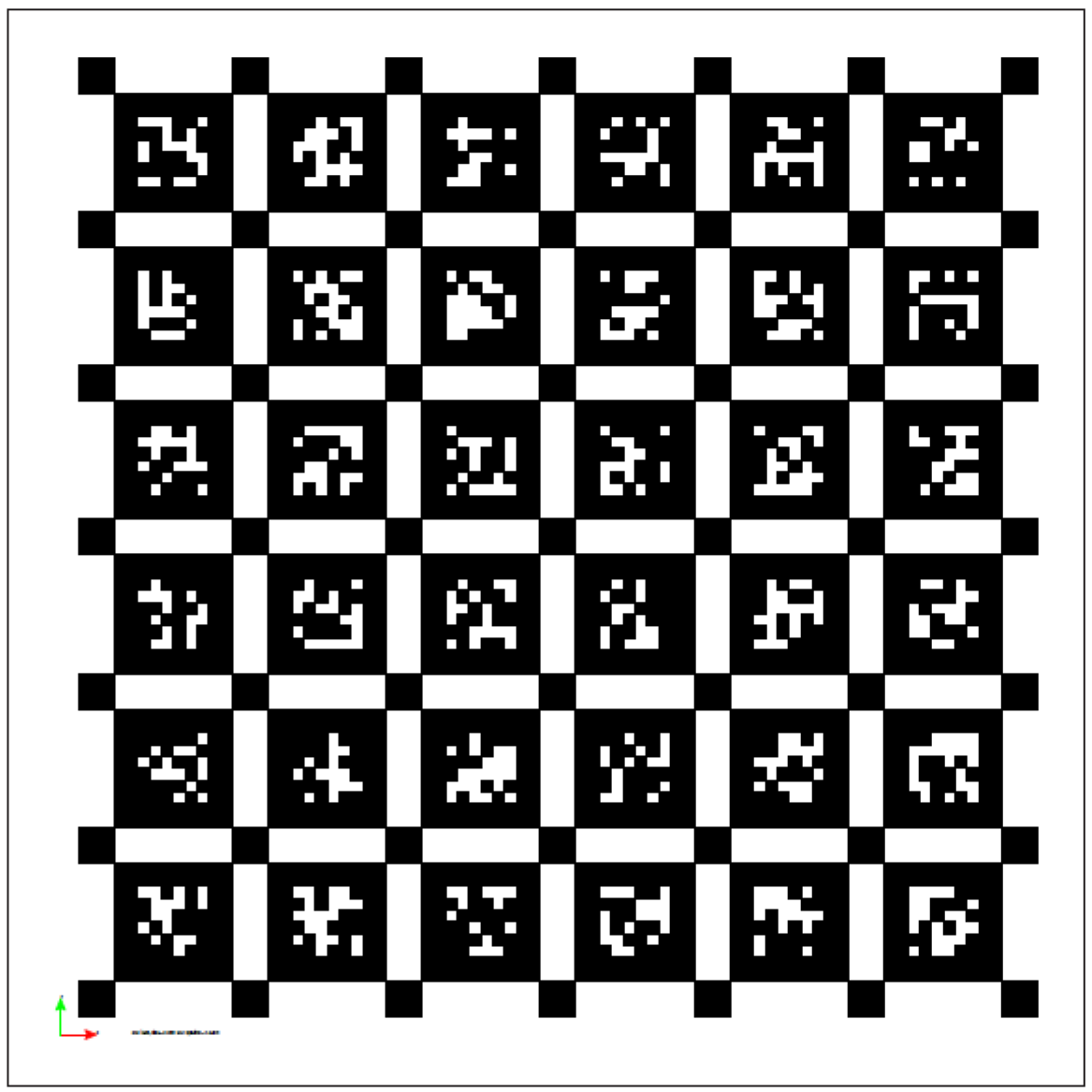
Figure 8.
The targets used in the Measurement Laboratory and the frame of reference used for the measurements.
Figure 8.
The targets used in the Measurement Laboratory and the frame of reference used for the measurements.
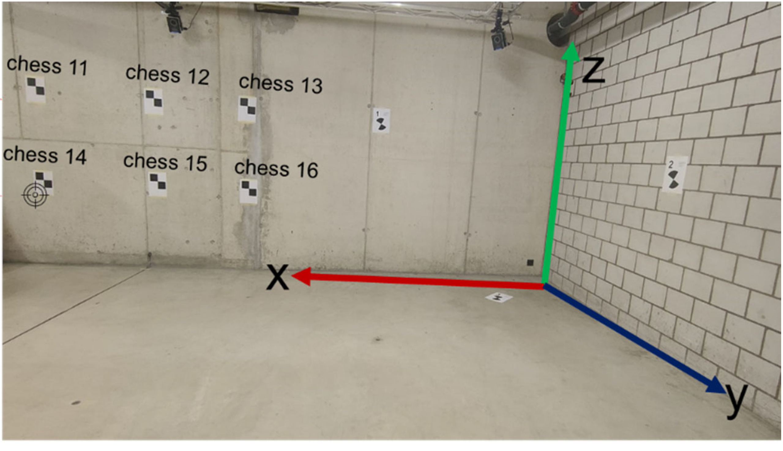
Figure 9.
The outdoor test area: the front side of the house (a) and the backside (b).
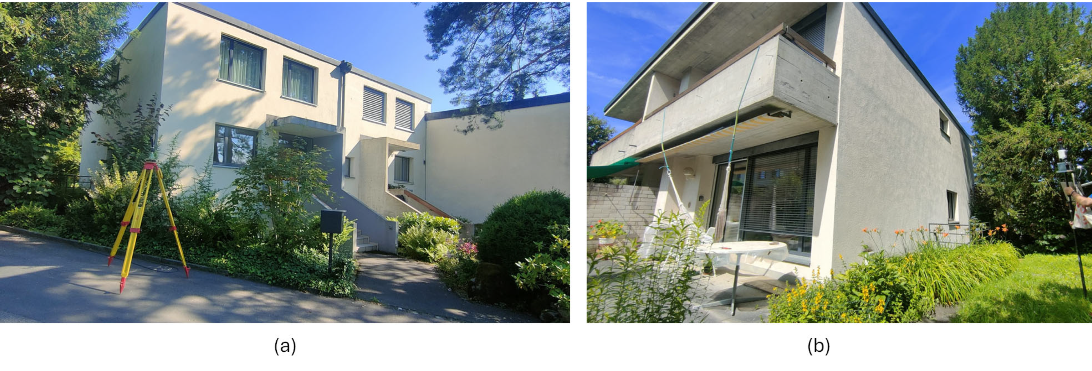
Figure 10.
The point cloud (3D scan) of the house taken by Leica RTC360.
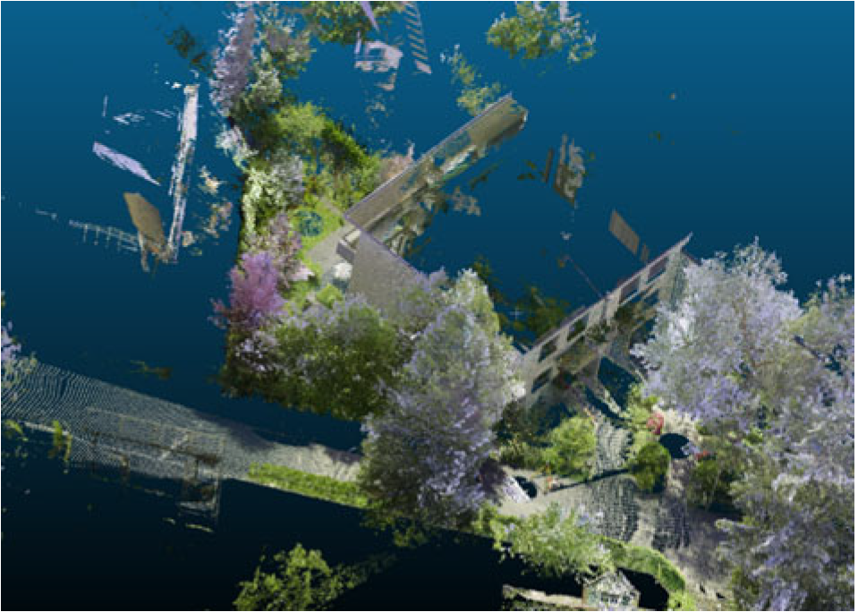
Figure 11.
The point cloud captured by the AP20-MSP (a) and with the GS18I-MSP (b) with a gradient blue-white-red scale [0-20 cm] with reference to RTC360 cloud. Points beyond 20 cm are shown in grey.
Figure 11.
The point cloud captured by the AP20-MSP (a) and with the GS18I-MSP (b) with a gradient blue-white-red scale [0-20 cm] with reference to RTC360 cloud. Points beyond 20 cm are shown in grey.

Figure 12.
Point cloud of a Laser scanning target taken by RTC360 (a), AP20-MSP (b), and GS18I-MSP (c).
Figure 12.
Point cloud of a Laser scanning target taken by RTC360 (a), AP20-MSP (b), and GS18I-MSP (c).
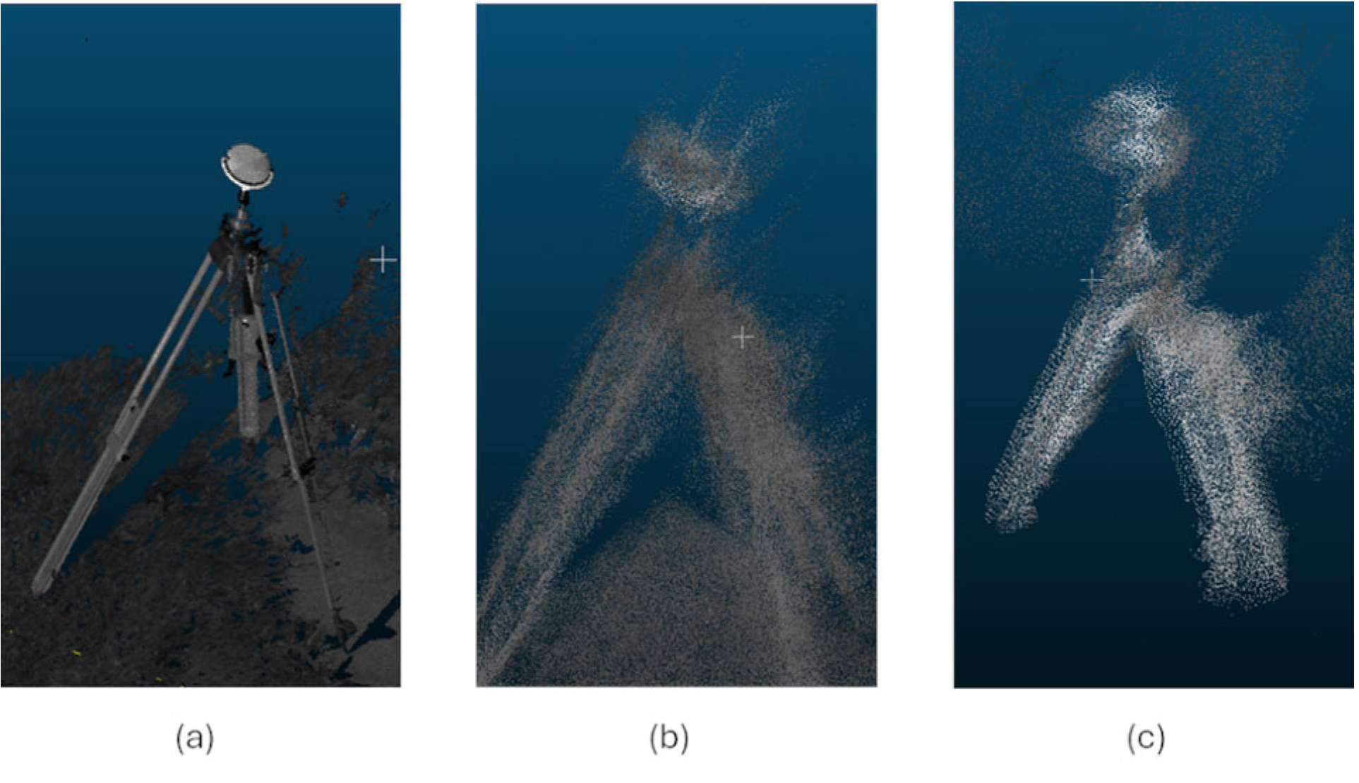

Table 1.
Relative distances with the AP20-MSP taken inside the point clouds. The MS60 was setup at point hp2.
Table 1.
Relative distances with the AP20-MSP taken inside the point clouds. The MS60 was setup at point hp2.
| Relative Euclidean Distances | Reference (cm) | AP20-MSP (cm) | Absolute Difference (cm) |
|---|---|---|---|
| hp1 - hp3 | 2152.16 | 2150.95 | 1.21 |
| hp1 - b1 | 1511.78 | 1527.12 | 15.34 |
| hp1 - w1 | 476.27 | 479.23 | 2.96 |
| hp3 - b1 | 703.19 | 693.36 | 9.83 |
| hp3 - w1 | 1736.68 | 1733.14 | 3.55 |
| b1 - w1 | 1139.66 | 1154.83 | 15.17 |
Table 2.
Relative distances measured in the case of GS18I-MSP.
| Relative Distances | Reference (cm) | GS18I (cm) | Difference (cm) |
|---|---|---|---|
| hp10 - hp11 | 837.1019054 | 847.1367308 | 10.0348255 |
| hp10 - hp12 | 2151.075994 | 2153.074596 | 1.9986027 |
| hp10 - hp13 | 1727.61305 | 1715.905781 | 11.7072688 |
| hp10 - b1 | 1600.911458 | 1602.782932 | 1.8714743 |
| hp10 -w1 | 528.2080972 | 528.1254348 | 0.0826624 |
| hp11 - hp12 | 2074.36564 | 2084.60091 | 10.2352697 |
| hp11 -hp13 | 1230.671999 | 1228.475154 | 2.1968451 |
| hp11 - b1 | 1367.57974 | 1383.822875 | 16.2431352 |
| hp11 - w1 | 535.6250931 | 527.0658504 | 8.5592427 |
| hp12 - hp13 | 1147.739082 | 1139.297083 | 8.4419986 |
| hp12 -b1 | 733.5967596 | 725.9267146 | 7.670045 |
| hp12 - w1 | 1770.374408 | 1791.66908 | 21.2946712 |
| hp13 -b1 | 525.1244827 | 527.4907236 | 2.366241 |
| hp13 - w1 | 1223.509798 | 1218.587109 | 4.9226889 |
| b1 - w1 | 1139.664807 | 1157.596949 | 17.9321426 |
Table 3.
AP20-MSP absolute measurements compared to MS60 Reference Points.
| Point | x Error (cm) | y Error (cm) | z Error (cm) | 2D Error (cm) | 3D Error (cm) |
|---|---|---|---|---|---|
| hp1 | 2.357000019 | 0.188999996 | 1.2724951 | 2.364565518 | 2.6852214 |
| hp3 | 2.581000002 | -1.124999998 | -0.8295166 | 2.815525885 | 2.9351804 |
| b1 | -14.35180004 | 6.526800012 | -2.4416104 | 15.76620699 | 15.954145 |
| w1 | 2.805700013 | 3.2289 | 1.03129 | 4.277586676 | 4.4001485 |
Table 4.
Absolute measurement accuracy in the GS18I-MSP.
| Point | x Error (cm) | y Error (cm) | z Error (cm) | 2D Error (cm) | 3D Error (cm) |
|---|---|---|---|---|---|
| hp10 | 36.38672149 | 16.22935991 | -3.450019984 | 15.85842001 | -21.06687547 |
| hp11 | 34.1634389 | 6.73135915 | -6.705598999 | 0.588335004 | -21.99372122 |
| hp12 | 25.51609074 | 16.98339216 | -14.63164198 | 8.622683003 | -7.542984988 |
| hp13 | 24.9062183 | 15.59327083 | 7.357353996 | 13.748434 | -7.920855154 |
| b1 | 32.47927548 | 20.96398079 | -2.111156005 | 20.85740902 | -24.80755622 |
| w1 | 27.82355144 | 11.8382807 | -5.853836006 | -10.289679 | -25.17945839 |
Disclaimer/Publisher’s Note: The statements, opinions and data contained in all publications are solely those of the individual author(s) and contributor(s) and not of MDPI and/or the editor(s). MDPI and/or the editor(s) disclaim responsibility for any injury to people or property resulting from any ideas, methods, instructions or products referred to in the content. |
© 2025 by the authors. Licensee MDPI, Basel, Switzerland. This article is an open access article distributed under the terms and conditions of the Creative Commons Attribution (CC BY) license (http://creativecommons.org/licenses/by/4.0/).
Copyright: This open access article is published under a Creative Commons CC BY 4.0 license, which permit the free download, distribution, and reuse, provided that the author and preprint are cited in any reuse.


