
Submitted:
28 June 2023
Posted:
29 June 2023
You are already at the latest version
Abstract
Commercially available multispectral and thermal imagers are commonly deployed for environmental monitoring on small uncrewed aerial systems (sUAS, <55 lbs). Our team assessed the challenges of deploying these imagers on a Group 3 classification UAS (weight: 55-1320 lbs, maximum altitude: 18,000 ft MSL, maximum speed: 250 kts) for the purpose of land-atmosphere interaction studies. A Micasense Altum multispectral imager was deployed on two very similar mid-sized (Group 3) UAS, a Mississippi State University (MSU) TigerShark XP and the Department of Energy (DOE) ArcticShark. This paper examines the effects of flight on imaging systems mounted on UASs flying at higher altitudes, faster speeds, and for longer duration, which near future technology will make more the norm. For these platforms we found that the acquisition rate may need to be higher to achieve a minimum 75% overlap, as required by certain post-processing algorithms. Additionally pre-flight calibration panel referencing was found to be problematic for converting flight images to reflectance, due to the changing illumination conditions during the extended duration flights. We developed an automated workflow to correct the image frames via data from an onboard hemispherical solar sensor mounted on the top of the airframe, and we assessed these data against known spectral ground targets and independent sources. Finally, this manuscript may be used as a reference for collecting similar datasets in the future. The datasets described within this manuscript may be used as a starting point for future research.
Keywords:
UAS operations
; land-atmosphere interactions
; automated processing
1. Introduction
Datasets for assessing land-atmospheric interactions have largely relied on two sources: satellite imagery and in situ surface measurements (towers). Land surface imagery traditionally used in atmospheric research comes from earth observation satellites including, the Moderate Resolution Imaging Spectroradiometer (MODIS), Landsat, Sentinel-2, and other government operated systems. These systems operate in sun-synchronous polar orbits and continually collect data at varying resolutions and revisit times. While valuable, these systems may not be suitable for applications which require temporal control and high spatial resolution.
Scientists in the field of land-atmosphere interactions and boundary layer meteorology traditionally rely on information from flux or eddy covariance towers to determine the surface energy balance (Aubinet et al., 2012), by deploying a net radiometer and sonic anemometer to capture the relevant parameters.
While tower instrumentation is not weight or power constrained, its fixed location at a single altitude limits its measurements to the surrounding environment. Conversely, satellite observational data provide a spatially distributed measure at a regional to global scale but are limited to revisit times determined by the satellite’s orbit and cloud cover. Some studies, however, require aerial measurements across a wider area than towers can provide, at a cadence and schedule that satellites cannot match.
One recent advancement to fill this gap has been the use of sUAS (<55lbs) with multispectral imager payloads. These multispectral imagers have been tested thoroughly on sUAS and have been featured in numerous publications (Brenner et al., 2017; Sankaran et al., 2018; Simpson et al., 2021). These systems offer an advantage over satellite imagery for their ability to provide thermal and visible imagery at higher resolution (~4 cm/pixel) and have been deployed successfully in the areas of precision agriculture, forestry, and civil engineering (Baena et al., 2017; Khaliq et al., 2019; Mishra et al., 2012; Nassar et al., 2018). They are quick to deploy and redeploy, fly generally up to an altitude of 120 m Above Ground Level (AGL) with a battery life of 20-40 minutes capturing surface imagery at a ground speed of ~15 m/s. These imagers usually capture RGB, red edge, and near infrared (NIR), but some are equipped to synchronically collect thermal imagery (long wave infrared; LWIR) while others collect in hyperspectral wavelengths. The thermal imagery collected via sUAS provides greater surface detail than infrared thermometers deployed on the same sUAS, because the thermal imagers measure skin temperature for every pixel within the field of view. The raw image frames are aligned and stitched together to create high resolution image products, which are rectified via ground control points to create orthomosaics. Using the technique of structure from motion the processing software can also create digital elevation models of the bare ground and canopy surface (Westoby et al., 2012). The calibrated multispectral data can be combined to derive atmospherically relevant surface properties such as albedo, surface reflectance, skin temperature, and various vegetative indices. It has been demonstrated that calibrated orthomosaics with one or two source energy budget models can be used to map surface radiation, improving upon the single point source that a flux station provides (Nieto et al., 2019).
However, sUAS do have disadvantages. These include limited surface area coverage (though an improvement from fixed stations) and their impracticability for some atmospheric science applications, as they provide a spatial resolution orders of magnitude higher than what may be incorporated into even fine scale atmospheric models. A better platform for many atmospheric science applications is a mid-size (Group 3) UAS (>55 lb and <1,320 lb) that can deploy continuously for multiple hours, 1 to 2 times a day and can image an area on the order of cloud resolving model spatial boundaries at a spatial resolution on the order of ~1-10 m.
Programmable flight plans used to control UAS enable routine and precise surface capture with accurate repeatability. However, there are challenges with deploying these imagers on a mid-size UAS. Land surface images taken from higher altitudes may introduce artifacts from aerosol and water vapor scattering/absorption in the air column. When flying for longer durations, there will be fluctuations in irradiance due to changing solar angle and variability in the aerosol and water vapor concentration. In addition, the aircraft will experience stronger winds aloft causing a large difference in ground speed as the aircraft experience headwinds and tailwinds. And a fixed wing midsize UAS is not as nimble as a small UAS. Thus, the aircraft will spend more time maneuvering to line up with the next sample line.
In this paper we address these challenges directly, evaluating calibration methodologies including the use of reflectance tarps along our flight path for empirical line fit reflectance corrections. Different flight planning strategies and image capture techniques that ensure proper image overlap and capture with minimal time in the air are presented. The utilization of the data from the downwelling light sensor version 2 (DLS2) to correct for changing solar illumination conditions is discussed. An intercomparison of the Altum thermal sensor covering the same wavelength and a similar field of view (FOV) with thermal imager onboard the UAS is also shown. Finally, we present orthomosaics generated in flight and propose future work and application of this dataset.
2. Methods
The data presented here were captured during flights with Group 3 UAS in November 2021 over the Department of Energy Atmospheric Radiation Measurement (ARM) Southern Great Plains (SGP) site and in February 2023 within the Pendleton, Oregon, UAS Range (PUR). The imager used in all flights is the Altum developed by MicaSense. The post processing routine was developed at Pacific Northwest National Laboratory (PNNL) using elements from MicaSense’s python tools and the United State Geological Survey’s guide to structure-from-motion photogrammetry using the imagery processing software Agisoft MetaShape (Over et al., 2021). The final imagery products are orthomosaics.
2.1. Mid-size UAS description
The ARM Aerial Facility (AAF, Schmid et al., 2014) has been operating the Navmar Science Corporation (NASC) ArcticShark Uncrewed Aerial System (UAS) since 2017 (de Boer et al., 2018). The ArcticShark which is a custom-built variant (TS-B3-XP-AS) of the standard TigerShark Block 3 (TS-B3-XP) UAS. While the ArcticShark was undergoing upgrades and modifications in 2021, the AAF staff collaborated with the Mississippi State University (MSU) Raspet Flight Research Laboratory (RFRL) to fly the ArcticShark scientific payload on a RFRL TS-B3-XP TigerShark. A description of the datasets obtained from the AAF payload can be found here (Mei et al., 2022). A comparison between the TigerShark XP and ArcticShark is shown in the table below.

Table 1.
Description of mid-size UAS used.
| TigerShark XP | ArcticShark | |
|---|---|---|
| Engine | Herbrandson 337 | UEL 801 |
| Payload power available | 800 W | 2500 W |
| Wingspan | 22 | 22 |
| Payload Weight (max, lb) | 50 | 100 |
| Gross Weight (lb) | 515 | 650 |
| Time Aloft (payload and flight profile dependent) |
8-10 hours | 8 hours |
| Typical True Airspeed (kts) | 63 | 63 |
| Nose type | Streamline | Bulbous |
The aircraft is operated using Cloud Cap’s Piccolo autopilot, which allows for repeatable, pre-programmed flight plan execution. The autopilot produces a log of aircraft performance variables including pitch, roll, and yaw, which can be compared to the imager’s metadata.
2.2. Altum Imager and Calibration
The MicaSense Altum imager is a commercial off the shelf, synchronized multispectral and thermal camera, combined with a GPS unit and downwelling light sensor (MicaSense, 2020). The Altum sensor captures multispectral images of the land surface across five optical bands (480 HFOV x 36.80 vertical FOV (VFOV)) and one long-wave infrared thermal band (570 HFOV x 44.30 VFOV). The spectral bands details are shown in Table 3. In the optical bands, the sensor measures reflected radiance and converts it to digital numbers via calibration coefficients. The emitted thermal data are recorded in the same manner.
The imager was mounted to the ventral side of each aircraft in the main payload bay. The camera was installed in the payload bay in a custom 3D printed case in the “landscape” position, such that the HFOV was maximized for image overlap. The DLS2 light sensor was mounted on the dorsal side of the aircraft on a custom plate parallel to the aircraft’s angle of attack, from which it could be easily unclipped for pre-flight magnetometer calibrations. Additional epoxy was added to the cable to improve robustness.
For our configuration, we used the DLS2′s integrated GPS for positional accuracy. Images were captured in timer mode every 2 seconds which provides sufficient time for the completion of the automatic thermal non-uniformity correction (NUC) for changing internal temperature of the sensor. The imager was powered from the aircraft’s onboard data acquisition system. Horizontal overlap was accounted for with the preprogramed flight plan’s distance between lines. As we are near the threshold of the Altum’s fastest capture rate (1 Hz) overlap may be limited by the groundspeed.
The DLS2 also provided synced measurements of direct and diffuse irradiance and sun to sensor angle. This information was recorded in the metadata of the TIFF images. We used these measurements to correct for changing lighting conditions along the flight path (such as changing cloud cover).
The standard calibration practice for an Altum multispectral camera is to take a pre and post flight image of a calibration panel (15x15 cm) of known reflectance that is provided by Micasense (Figure 1). However, this method was infeasible for a mid-size UAS. To image the panel, the entire platform had to be tilted, resulting in different incoming solar incidence angles for the DLS unit and the panel. Additionally, post-flight panel captures with both the DLS2 and panel in sunlight were not possible due to the high solar elevation angle and the bulbous nose of the ArcticShark. This calibration method is no longer used. Instead, Tetracam™ calibration tarps with 11% and 48% absolute reflectance in the range of 400 nm to 850 nm are routinely imaged by the camera while in flight. This can provide a far more accurate calibration that incorporates any impacts from aerosol and water vapor
For validation of the Micasense™ thermal imager, a ventral Apogee SI-411-SS infrared thermometer (IRT), with a 440 FOV was flown. The Apogee IRT samples 60% of the Altum thermal sensor surface area. In our sampling area there was a 25 m and 10 m tower with a down-looking IRT (Heitronics 700) at the DOE ARM Southern Great Plains atmospheric observatory. These Apogee and Heitronics IRTs have been compared over asphalt with good agreement (Krishnan et al., 2020).
One feature of operation which differed greatly between operating this camera on a sUAS and a midsize UAS was the treatment of target altitude. sUAS are generally flown under 14 CFR part 107 guidelines to a maximum altitude of 120 m (400 ft). Therefore, altitude control of these platforms by their autopilot is treated as a range between target altitude and a lower limit (target altitude – X). For larger aircraft, the programmed altitude is thought of having a tolerance range treated as target altitude ± X. The Altum imager’s capture range is designed to be programmed in using the sUAS method. Therefore, to set the Altum’s image capture to match the midsize UAS’s flight altitude, we used the following formula:
true target altitude = programmed target altitude – X ft
X = desired range above and below target altitude
programmed range = 2*X
2.3. Flight Patterns
The objective of the pre-programmed flight pattern is to acquire images with sufficient overlap between frames to derive a topographic surface and minimize the time aloft. The completion of the acquisition as quickly as possible minimizes the change in solar and atmospheric conditions. For these deployments, a flight pattern commonly referred to as a “lawn mower” was used to capture imagery across a broad area. Initial flight patterns had the ArcticShark fly the sampling legs sequentially and covered an area of 10 km2. At 2,000 ft AGL, the flight legs were 95 m apart to maintain 75% overlap between adjacent images (Figure 2). Because the turning radius of the aircraft significantly exceeds 0.5 * 95 m, this flight pattern resulted in rapid, banked (teardrop) turns at the end of the lines. This additional maneuvering greatly increased the flight time resulting in 90 minutes for completion.
A more efficient method is to fly an alternating leg pattern where the turns can be planned to match the mid-size UAS turning radius. This alternating leg flight plan was theoretically tested in the ArcticShark’s Piccolo flight simulator developed by Cloud Cap. For a 9.2 km2 coverage, the flight is predicted to take an estimated 60 minutes at 2000 ft and at 4000 ft, with spacing between legs reduced to 200, it would take 30 minutes to complete. During flight operations in February 2023, the ArcticShark flew an alternating leg pattern (Figure 2) at 3,000 ft AGL covering 7 km2 in 45 minutes verifying the flight simulator estimates. This amount of time is nominally the same as it takes to capture a 1 km2 area via a sUAS platform.
Horizontal overlap was solely dependent on HFOV, the aircraft altitude, and the width of the flight legs, both of which are known before flight. The forward overlap was dependent on VFOV, the aircraft altitude, and ground speed. As only true airspeed (TAS) can be programmed by the Piccolo autopilot, the ground speed could be variable in flight due to winds aloft, thus there is no single capture rate that could be used to precisely maintain 75% overlap throughout the flight. To ensure the capture rate at a planned flight altitude is equal to or greater than 2s, the capture rate is calculated by the following equation:
Tcapture = capture rate (s)
Gs= ground speed (m/s)
O = fractional overlap (e.g., 0.75 = 75%)
A = altitude (m)
VFOV = vertical field of view
Table 2.
Estimated capture rates, using a ground speed of 33 m/s (64 kts) and 75% overlap. A ground speed of 33 m/s assumes there is no influence from winds.
Table 2.
Estimated capture rates, using a ground speed of 33 m/s (64 kts) and 75% overlap. A ground speed of 33 m/s assumes there is no influence from winds.
| AGL (m) | AGL (ft) | Capture Rate (s) |
|---|---|---|
| 609 | ~2000 | 3.1 |
| 914 | ~3000 | 4.6 |
| 1220 | ~4000 | 6.1 |
The variability in the ground speed, however, can be reduced by flying perpendicular to the wind direction as shown in Figure 2. During flight operations in February 2023, this methodology was successfully demonstrated with the aircraft flying at a TAS of 33.3 +/- 1 m/s in 15 m/s winds from 2230. The heading of the legs (1550 and 3350) was determined utilizing the North America Model (NAM) prediction of a winds from 2450. Although this prediction was slightly incorrect, the ground speed on the 1550 legs was 26 +/- 1.4 m/s and on the 3350 legs was 37.5 +/- 1.6 m/s. This 11.6 m/s difference in ground speed was ~3 times better than the 30 m/s expected difference had the aircraft flown parallel to the winds. The aircraft average crab angle (difference in the yaw direction from the heading) of 24.8 +/- 40 had no impact on the ability to generate a merged mosaic.
2.4. Post Processing
Imagery to be used in science applications should be radiometrically corrected considering the sensor calibration, lens distortions, vignette effects, sun angle, and atmospheric effects (scattering and absorption). The standard operating procedure to convert UAS multispectral data to reflectance is to take pre- and post-flight measurements over an anisotropic target with known spectral properties (panels mentioned in section 2.3). These measurements are then used to calculate a coefficient to convert the DN directly to reflectance for each band. Successful use of this procedure assumes that incoming solar radiation remains constant during the flight. Such an assumption is frequently justified when flying short missions over small areas (10-20 minutes) but becomes problematic for longer missions or those taking place under partial cloud cover. Neither assumption is met for our application, requiring the development of an alternate processing workflow for the Micasense data. Since the longer flight times of mid-sized UAS results in changing solar conditions, the DLS data can be used directly to calculate the apparent reflectance for each image frame. Using the DLS sensor which measures incoming solar irradiance at the precise time of image capture, we can estimate reflectance by ratioing the DLS band spectral irradiance value to the radiance measured at the sensor (Equation 3 below).
Rλ=π × Lλ/ Iλ
Rλ = band reflectance
Lλ = band radiance from image
Iλ = band irradiance from DLS
These data were further corrected by referencing the reflectance tarp values to determine empirical line fit coefficients for each band specific to a particular flight altitude. Since time between altitudes is a small portion of total flight time, the changes in solar irradiance are minimized. The corrected images were then input to the photogrammetry software Agisoft Metashape v 1.4 to align and stitch the images into a larger composite image. The images have a resolution of 20-60 cm/pixel depending on the altitude at which taken, which are subsampled to 100 cm/pixel.
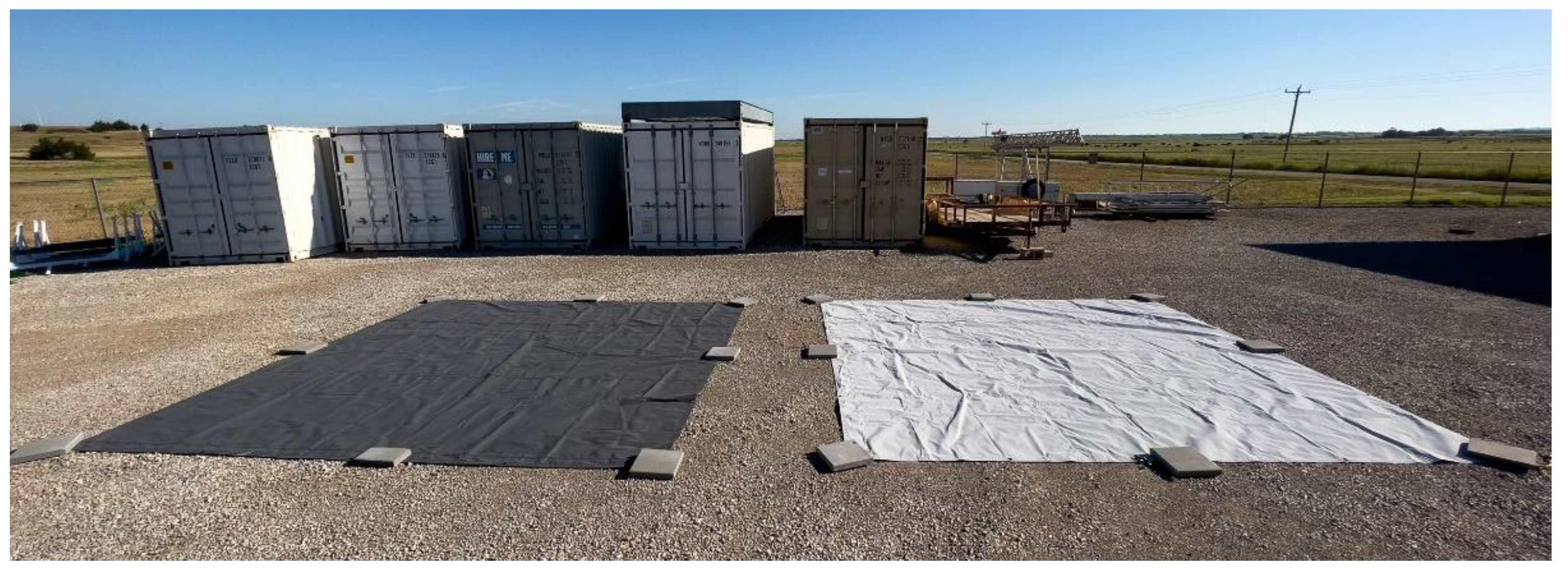
Figure 3.
Field deployment of calibration tarps. Leftmost tarp is 11% reflectance, 48% reflectance on right.
Figure 3.
Field deployment of calibration tarps. Leftmost tarp is 11% reflectance, 48% reflectance on right.
Our processing script follows the published USGS workflow to apply the structure from motion image algorithm in Agisoft to construct a dense cloud and 3D model of the surface (Over et al. 2021). The 3D model is used to produce a raster digital elevation model (DEM) of the area of image capture.
The final mosaics can be used to calculate for leaf area index, albedo, and various other vegetative indices, such as Normalized Difference Vegetation Index (NDVI), Green Normalized Difference Vegetation Index (GNDVI), Normalized Difference Water Index (NDWI), surface temperature, and Enhanced Vegetation Index (EVI). From the thermal band a mosaic of skin surface temperature is produced and these measurements can be used to calculate evapotranspiration of vegetation crop stress indices.
We based our quantitative geometric and radiometric corrective schema on that described in Iqbal et al. 2018. The three-part semi-automated Python workflow we created is tailored for routine deployments, with user input required to specify the number flying levels and the location of calibration tarps. The first script runs the uncorrected imagery through the Micasense Python radiometric correction code so that the images are corrected for dark level, row gradient, and radiometric calibration to radiance. The second script uses Agisoft Metashape API code and automates the processes that would normally be done in the Agisoft Metashape GUI. Following the guidance of the USGS structure from motion workflow we added parameters for camera alignment and gradual selection (Westoby et al., 2012). We subsample our resolution to 1 m2/pixel for routine comparison across image capture at different altitudes. In the final part of the workflow, the empirical line fit is applied to the orthomosaics using radiance values for known reflectance tarps that are visible in the imagery.
While not entirely open source due to the licensing of Agisoft, our code is available for download via the ARM repository, and can be adapted for other imagery software APIs (such as Pix4d™), https://github.com/ARM-DOE/camspec-air-processing. Both the unprocessed imagery collected and the final processed orthomosaics are available for download from the ARM archive (https://adc.arm.gov/discovery/#/results/s::camspec-air).
3. Results
The quality of images taken with the Altum multispectral camera on a Group 3 UAS are discussed below. We found that this imager can collect surface data with the resolution and quality more than sufficient for atmospheric science research. The orthomosaics of the calibre we produced can be used to probe the effects of surface heterogeneity at cloud resolving scales.
3.1. Calibration
Instead of the calibration panel, tarps of known reflectance,11% and 48%, were overflown at multiple altitudes between 520 - 1360 m AGL (900 - 1740 m MSL). Tarp observations at different levels enabled the assessment of the effect of altitude on data quality. In addition, calibrations utilizing these tarps incorporate any impacts from aerosol and water vapor. Figure 4 shows the published tarp reflectance values as well as the mean 3x3 neighbourhood pixel values cantered on the tarps for each altitude collect. We would expect more pronounced atmospheric scattering in the shortest wavelengths, thus increasing the reflectance values in the corresponding bands. This effect would be especially noticeable over the dark target. We see no such increase in reflectance values over either tarp and in some cases a decrease was observed. The apparent difference between published tarp values and pixel values for the tarp images are likely due to noise in DLS2 measurements used to ratio the image radiance values to reflectance.
3.2. Data quality and validation
3.2.1. Thermal imagery comparison to infrared thermometers
The IRT flown on the TigerShark (and ArcticShark) was an Apogee SI-411-SS that senses surface skin temperature via a thermopile (Tomlinson et al. 2021). Like the Altum thermal band, it also measures in the 8-14 um wavelength range and has a similar FOV, allowing for excellent intercomparison between the sensors, as conducted in previous studies (Collatz et al., 2018). Serving as a further comparison, a 30m tower at the SGP site is equipped with an IRT sensor by Heitronics 700 (Howie et al. 2021). All three sensors were analysed for flights covering the tower area. The aircraft Apogee and stationary Heitronics IRT sensors were compared only when their FOV overlapped, demonstrating agreement within 0.250 C during the day. The comparison of the Apogee to the Altum thermal band showed that the Altum sensor was on average 50 C colder, which is consistent with the literature (Krishnan et al., 2020). We believe this is due to the thickness of the window on the thermal imager lens. Notably, Mei et al. found that the Apogee IRT surface temperature readings varied with altitude, likely resulting from changing internal temperature (Mei et al., 2022).
Figure 5.
November 13th, 2021 flight. Comparison of the the UAS IRT (vendor Apogee) to the ARM 30m tower based ground IRT (vendor Heitronics). Data points are compared when the FOV of the UAS IRT partially or totally overlapped with the ground IRT independent of altitude.
Figure 5.
November 13th, 2021 flight. Comparison of the the UAS IRT (vendor Apogee) to the ARM 30m tower based ground IRT (vendor Heitronics). Data points are compared when the FOV of the UAS IRT partially or totally overlapped with the ground IRT independent of altitude.
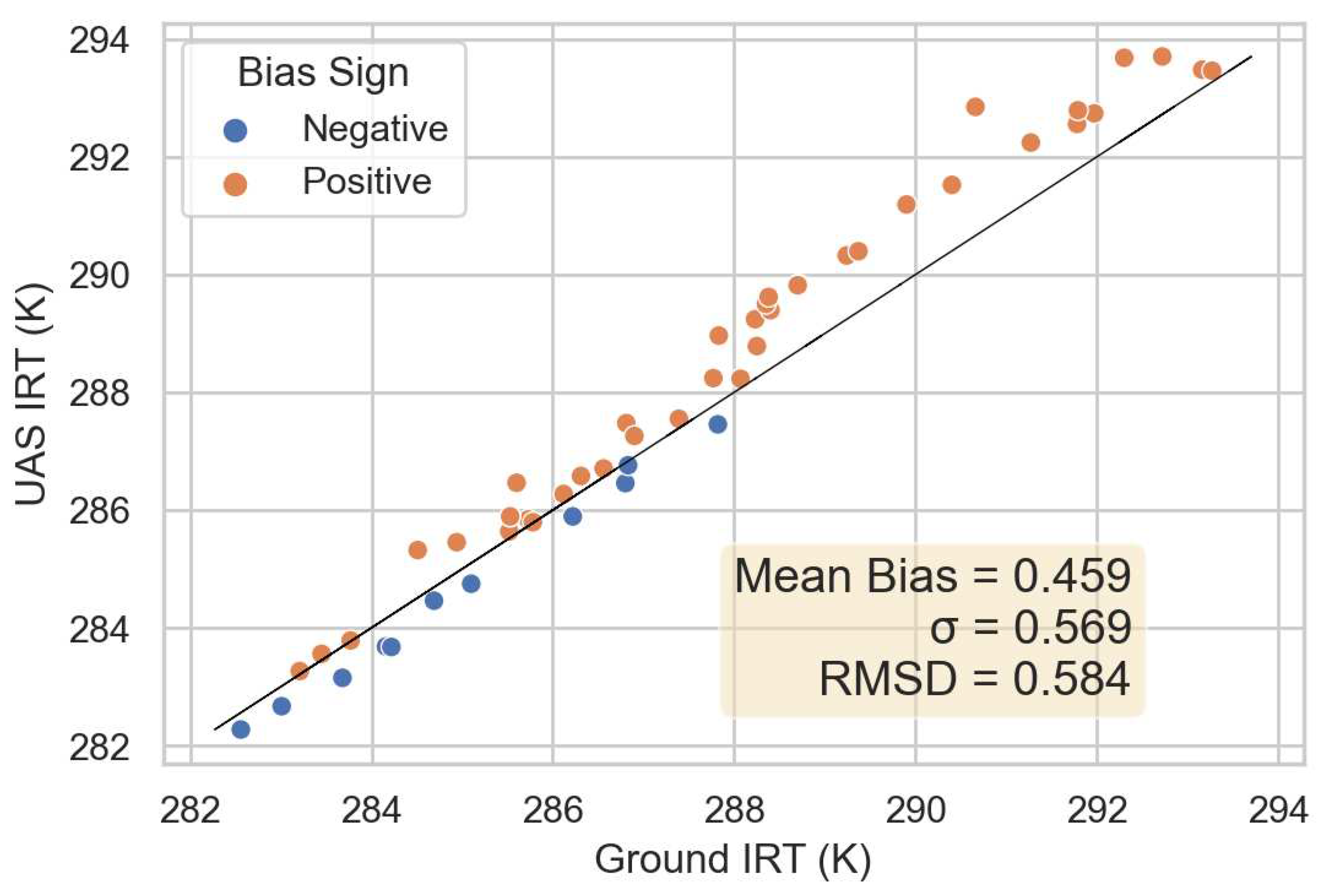
Referencing Figure 6, the aircraft flew a lawnmower pattern at 520 m AGL with the imager collecting images, and then a square based ladder pattern climbing up to 1360m AGL with the IRT in continuous operation. The reported surface temperature from the IRT decreased with altitude, affected by the colder temperatures with altitude (Mei et al. 2022). For the scatter plots, the thermal data within the FOV was averaged into a single point to compare the Altum thermal imagery with the IRT’s time series data. The Altum has a distinct cold bias. A) Bias at 520 m AGL B) Comparison of skin surface temperatures at 520 m AGL C) Bias at 1360 m AGL D) Comparison of skin surface temperatures at 1360 m AGL.
3.2.2. Multispectral imagery comparison to space-born multispectral and hyperspectral imagery
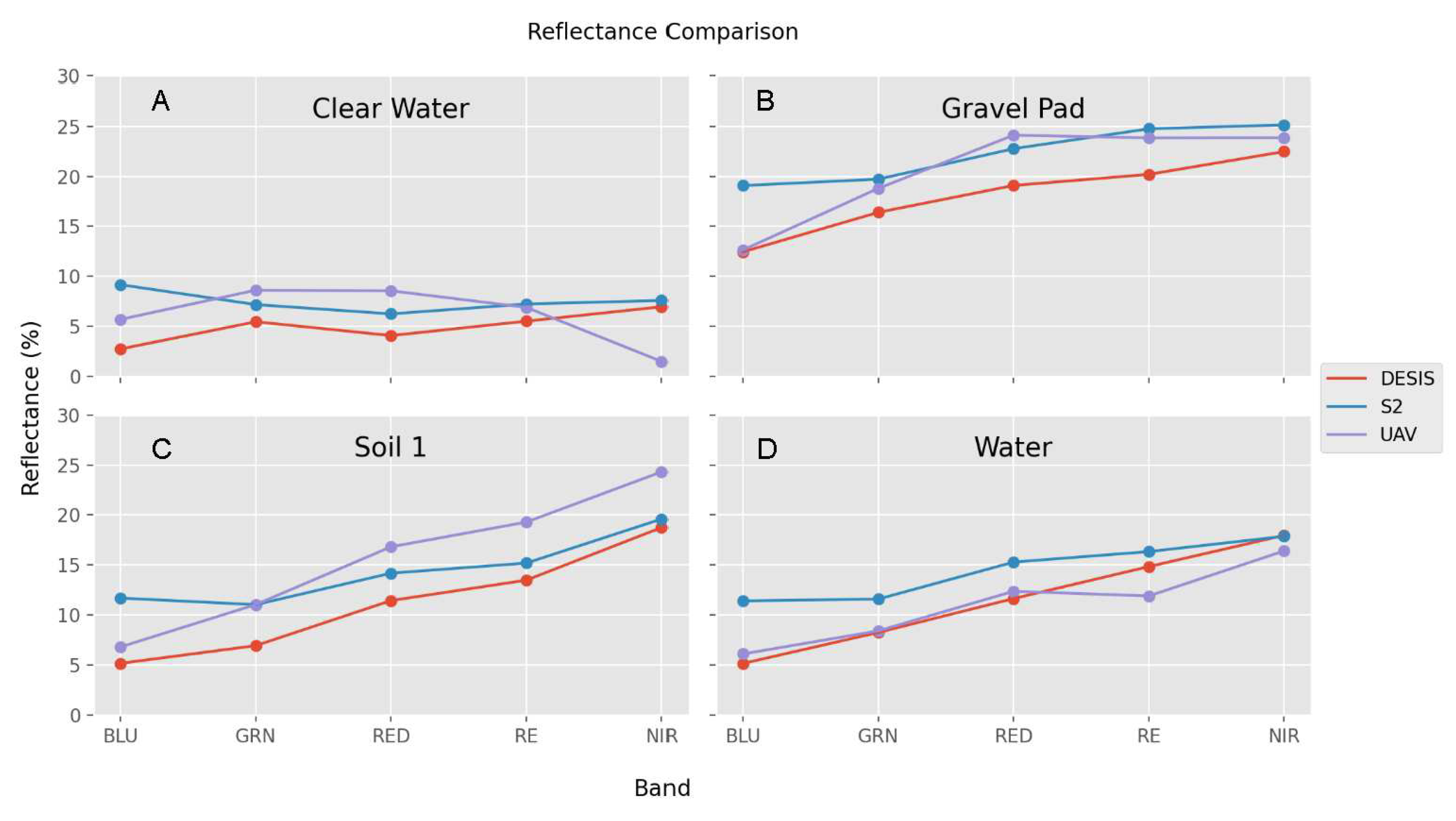
We compared the UAS imagery to satellite data over common ground features that were likely to be relatively stable - gravel pad, bare soil, and clear water. Two sources of multispectral satellite imagery were used for the comparison: DESIS and Sentinel-2. The DESIS hyperspectral sensor orbits on the US space station and collects data over the US at varying intervals. We downloaded a DESIS image for our area of interest, collected approximately 4 weeks before our mission (October 12, 2021). The DESIS sensor has 235 bands of data with 5 of those bands sharing a common wavelength as the center wavelength of Altum sensor bands. The Sentinel-2 platform operated by the European Space Agency (ESA) consists of two satellites in complementary orbits. Each satellite carries a wide swath high-resolution multispectral imager with 13 spectral bands and collects data at 10 - 60 m resolution every 5 days. We used Sentinel-2 data from an overpass on October 11, 2021.
Figure 7.
Comparison of UAS-acquired data to images from DESIS hyperspectral and Sentinel-2 (S2) sensors for common surfaces. The DESIS data were acquired 4 weeks before the UAS mission.
Figure 7.
Comparison of UAS-acquired data to images from DESIS hyperspectral and Sentinel-2 (S2) sensors for common surfaces. The DESIS data were acquired 4 weeks before the UAS mission.
3.2.3. Other attributes
When we qualitatively assess imagery by reviewing the mosaics, we see that geometric and radiometric properties are reasonable (Figure 8). With pre-programmed flight plans and the aircraft’s autopilot, we were generally able to achieve the necessary 75-80% image overlap required for aligning and mosaicking the images. The aircraft was able to maintain its flight path. Only at the highest altitude were the winds strong enough to elevate the ground speed where this overlap couldn’t be achieved. Otherwise, at a capture rate of 2 seconds, overlap was sufficient to avoid stretching and gaps in the orthomosaics. We opted to disable hole filling to ensure image distortion was minimized in the final mosaic.
We subsampled our image resolution to 1 m2 resolution. Geometric information is provided by the DLS GPS and Agisoft performs an image-to-image alignment. No artifacts of misalignment are evident in the mosaics created from the individual image frames. The rectified orthomosaics were shifted from known features up to an offset of 18 m. To reduce this offset, ground control points can either be placed pre-flight or selected from distinct feature in the image. Both methods would require human input to the workflow and were not employed here. Additionally, image-to-image methods were tested to align the UAS image with USGS orthophoto base, but results were variable. Further refinement of these approaches is needed for incorporation into future versions of the automated workflow.
3.2.4. Final Products
The final processed orthomosaics are available for download from the ARM archive (https://adc.arm.gov/discovery/#/results/s::camspec-air) (DOI: 10.5439/1894300, 10.5439/1894300, 10.5439/1962600). The reflectance imagery generated from each band can be combined via raster calculation to produce vegetative indices, which can inform on different aspects on the surface properties and biogenic matter below.
4. Data File Structure, Data Availability, and Code Availiability
The data is available at the ARM data repository and is free to download at adc.arm.gov. The spectral imagery data from the 2021 and 2022 UAS deployments are considered a “principle investigator” data product by the ARM Data management system. The data products name on the archive is “camspec-air”. As they are not considered “routine observation”, they don’t follow the ARM data file standards (Mather 2014). However, the data was submitted with best practices to follow the ARM standards and FAIR principles. The data is provided in tif and jpg format and uses the naming convention as follows:
{site}{instrument}.{YYYYMMDD}.{HHMMSS}.{altitude(msl)}.{file ext}
For the orthomosaic tif images, there are six bands represented per pixel that represent surface reflectivity (skin temperature for the sixth band). For the DEM, each pixel represents an elevation. Each pixel represents a 1 m2 area and has an associated latitude and longitude in the metadata. These images can be converted into gridded products that can be used for analysis. Raster calculations of these bands can provide information on albedo, leaf area index, skin temperature, and various vegetative indices (e.g., NDVI).
The raw images are available on the archive as well but are not publically displayed. To obtain a copy of the raw images, send an email directly to the ARM Data management center (adc@arm.gov) and the instrument mentor, Jerry Tagestad. An instrument webpage with a link to a handbook and a direct link to the data is here: https://arm.gov/capabilities/instruments/camspec-air. The code which was developed to process these images is available at the ARM Git repository: https://github.com/ARM-DOE/camspec-air-processing. While the code is open source, Agisoft Metashape is a licensed software that is needed for parts of the software to run. Other python libraries, which are free on line, are needed to make the script work.
The individual DOIs for these datasets are listed in table three. A description of the IRT data used in this analysis can be found in Mei et al. 2022.
Table 4.
DOI for main datasets.
| Date | Data product | Description | DOI |
|---|---|---|---|
| 11/2021 | GNDIRT | IRT 25M Infrared Thermometer: Ground surface temperature, averaged 60-second at 25-meter height. | 10.5439/1025205 |
| 11/2021 | AAFIRT | AAFIRT. ARM Aerial Facility- Unmanned Aircraft Systems, Tigershark (U3) | 10.5439/1821129 |
| 11/2021 | camspec-air | PI Data: Multispectral and Thermal Surface Imagery and Surface Elevation Mosaics (CAMSPEC-AIR) | 10.5439/1894300 |
| 07/2022 | camspec-air | PI Data: Multispectral and Thermal Surface Imagery and Surface Elevation Mosaics (CAMSPEC-AIR) | 10.5439/1962600 |
| 03/2023 | camspec-air | PI Data: Multispectral and Thermal Surface Imagery and Surface Elevation Mosaics (CAMSPEC-AIR) | 10.5439/1969041 |
5. Conclusion
This manuscript may be used as a future reference for flying imaging systems on mid-sized UASs. We found that the acquisition rate may need to be higher to assure 75% overlap, as required by certain post-processing algorithms, due to variable ground speeds caused by the more variable and stronger winds aloft. For best calibration practices, we found pre-flight calibration panel referencing was insufficient for converting flight images to reflectance, due to the changing illumination conditions during the extended flights. We instead recommend using reference ground tarps covering the expected reflectance range (11-48%), which the UAS can over fly while operating in the targeted area. We developed an automated post processing workflow to address changing lighting conditions and the high volume of imagery collected. We assessed these orthomosaics against independent sources and found good agreement. The data quality will be sufficient for informing and parameterizing surface conditions for atmospheric LES models. This effort represents a step towards expanding the application of multispectral and thermal imagers onto midsize UAS for atmospheric science research.
6. Team list for UAS Operations
Air Vehicle Pilots
- Stephen Hamilton, NASC
- Brad Petty, NASC
- Charley Zera, NASC
- Austin Wingo, MSU
Mission Commanders
- Pete Carroll, PNNL
- Nolan Parker, MSU
UAS Technicians
- Pete Carroll, PNNL
- Mike Crocker, PNNL
- Jonathan Stratman, PNNL
- Andre Watson, PNNL
- John Stephenson, PNNL
- Conor White, MSU
- Miles Ennis, MSU
Payload Operators
- Victor Aguilera-Vazquez, PNNL
Scientists
- Misha Pekour, PNNL
Director of Flight Operations
- Tim McLain, PNNL
Director of Maintenance
- Andre Watson, PNNL
Visual Observers
- Mike Hubbell, PNNL
- Lupita Renteira, PNNL
- Josh Torgenson, PNNL
- Orlando Garayburu-Caruso, PNNL
- Susanne Glienke, PNNL
- Eric Fischer, PNNL
- Clay Shires, MSU
- Randy Welch, MSU
- Cavin Skidmore, MSU
- Peter McKinley, MSU
- Taylor Eskridge, MSU
- Chase Jackson, MSU
Author Contributions
Lexie Goldberger-conceptualization and writing, Ilan Gonzalez-Hirshfeld- software, formal analysis, writing review and editing, Kristian Neilson-software, Hardeep Metha- investigation, Fan Mei-writing review, Jason Tomlinson-supervision, writing review and editing, Beat Schmid-funding acquisition, supervision, writing review and editing, Jerry Tagestad-data curation, writing review and editing.
Acknowledgements
This work has been supported by the Office of Biological and Environmental Research (OBER) of the US Department of Energy (DOE) via the Atmospheric Radiation Measurement (ARM) program.
Conflicts of Interest
The authors declare that they have no conflict of interest.
Special issue statement
By Journal if applicable.
References
- Aubinet, M.; Vesala, T.; Papale, D. (Eds.) Eddy Covariance; Springer: Netherlands, 2012. [Google Scholar] [CrossRef]
- Baena, S.; Moat, J.; Whaley, O.; Boyd, D.S. Identifying species from the air: UASs and the very high resolution challenge for plant conservation. PLoS ONE 2017, 12. [Google Scholar] [CrossRef] [PubMed]
- Brenner, C.; Thiem, C.E.; Wizemann, H.D.; Bernhardt, M.; Schulz, K. Estimating spatially distributed turbulent heat fluxes from high-resolution thermal imagery acquired with a UAV system. International Journal of Remote Sensing 2017, 38. [Google Scholar] [CrossRef] [PubMed]
- Collatz, W.; McKee, L.; Coopmans, C.; Torres-Rua, A.F.; Nieto, H.; Parry, C.; Elarab, M.; McKee, M.; Kustas, W. Inter-comparison of thermal measurements using ground-based sensors, UAV thermal cameras, and eddy covariance radiometers. In J. A. Thomasson, M. McKee, & R. J. Moorhead (Eds.), Autonomous Air and Ground Sensing Systems for Agricultural Optimization and Phenotyping III. SPIE. 2018. [CrossRef]
- de Boer, G.; Ivey, M.; Schmid, B.; Lawrence, D.; Dexheimer, D.; Mei, F.; Hubbe, J.; Bendure, A.; Hardesty, J.; Shupe, M.D.; et al. A Bird’s-Eye View: Development of an Operational ARM Unmanned Aerial Capability for Atmospheric Research in Arctic Alaska. Bulletin of the American Meteorological Society 2018, 99, 1197–1212. [Google Scholar] [CrossRef]
- Howie, J.; Goldberger, L.; Morris, V. IRT 25M Infrared Thermometer: Ground surface temperature, averaged 60-second at 25-meter height. (11/13/2021-11/15/2021). ARM Data Center [Dataset]. DOI: 10.5439/1025205. https://arm.gov/capabilities/instruments/irt, 2021.
- Iqbal, F.; Lucieer, A.; Barry, K. Simplified radiometric calibration for UAS-mounted multispectral sensor. European Journal of Remote Sensing 2018, 51. [Google Scholar] [CrossRef]
- Khaliq, A.; Comba, L.; Biglia, A.; Ricauda Aimonino, D.; Chiaberge, M.; Gay, P. Comparison of satellite and UAS-based multispectral imagery for vineyard variability assessment. Remote Sensing 2019, 11. [Google Scholar] [CrossRef]
- Krishnan, P.; Meyers, T.P.; Hook, S.J.; Heuer, M.; Senn, D.; Dumas, E.J. Intercomparison of In Situ Sensors for Ground-Based Land Surface Temperature Measurements. Sensors 2020, 20, 5268. [Google Scholar] [CrossRef] [PubMed]
- Mather, J. Introduction to Reading and Visualizing ARM Data, DOE Office of Science Atmospheric Radiation Measurement (ARM) Program …, 2013. DOE/SC-ARM-TR-136. 1. 1.0.
- McKee, M. The remote sensing data from your UAV probably isn’t scientific, but it should be! SPIE Commercial + Scientific Sensing and Imaging, 2017. [Google Scholar] [CrossRef]
- McKee, M.; FTorres-Rua, A.; Aboutalebi, M.; Nassar, A.; Coopmans, C.; Kustas, W.; Gao, F.; Dokoozlian, N.; Sanchez, L.; MAlsina, M. Challenges that beyond-visual-line-of-sight technology will create for UAS-based remote sensing in agriculture (Conference Presentation). Autonomous Air and Ground Sensing Systems for Agricultural Optimization and Phenotyping IV 2019.
- Mei, F.; Pekour, M.; Dexheimer, D.; de Boer, G.; Cook, R.; Tomlinson, J.; Schmid, B.; Goldberger, L.; Newsom, R.; Fast, J. Observational data from uncrewed systems over Southern Great Plains. Earth System Science Data 2022. [CrossRef]
- MicaSense. MicaSense Altum and DLS2 Integration Guide. MicaSense. 2020.
- Mishra, D.R.; Cho, H.J.; Ghosh, S.; Fox, A.; Downs, C.; Merani PB, T.; Kirui, P.; Jackson, N.; Mishra, S. Post-spill state of the marsh: Remote estimation of the ecological impact of the Gulf of Mexico oil spill on Louisiana Salt Marshes. Remote Sensing of Environment 2012, 118. [Google Scholar] [CrossRef]
- Nassar, A.; Aboutalebi, M.; McKee, M.; Torres-Rua, A.F.; Kustas, W. Implications of sensor inconsistencies and remote sensing error in the use of small unmanned aerial systems for generation of information products for agricultural management. In J. A. Thomasson, M. McKee, & R. J. Moorhead (Eds.), Autonomous Air and Ground Sensing Systems for Agricultural Optimization and Phenotyping III. SPIE. 2018. [CrossRef]
- Nieto, H.; Kustas, W.P.; Torres-Rúa, A.; Alfieri, J.G.; Gao, F.; Anderson, M.C.; White, W.A.; Song, L.; Alsina M del, M.; Prueger, J.H.; McKee, M.; Elarab, M.; McKee, L.G. Evaluation of TSEB turbulent fluxes using different methods for the retrieval of soil and canopy component temperatures from UAV thermal and multispectral imagery. Irrigation Science 2019, 37, 389–406. [Google Scholar] [CrossRef] [PubMed]
- Over, J.-S.R.; Ritchie, A.C.; Kranenburg, C.J.; Brown, J.A.; Buscombe, D.D.; Noble, T.; Sherwood, C.R.; Warrick, J.A.; Wernette, P.A. Processing Coastal Imagery With Agisoft Metashape Professional Edition, Version 1.6—Structure From Motion Workflow Documentation. 2021. [Google Scholar]
- Sankaran, S.; Zhou, J.; Khot, L.R.; Trapp, J.J.; Mndolwa, E.; Miklas, P.N. High-throughput field phenotyping in dry bean using small unmanned aerial vehicle based multispectral imagery. Computers and Electronics in Agriculture 2018, 151, 84–92. [Google Scholar] [CrossRef]
- Schmid, B.; Tomlinson, J.M.; Hubbe, J.M.; Comstock, J.M.; Mei, F.; Chand, D.; Pekour, M.S.; Kluzek, C.D.; Andrews, E.; Biraud, S.C.; McFarquhar, G.M. The DOE ARM Aerial Facility. Bull. Amer. Meteor. Soc. 2014, 95, 723–742. [Google Scholar] [CrossRef]
- Simpson, J.E.; Holman, F.; Nieto, H.; Voelksch, I.; Mauder, M.; Klatt, J.; Fiener, P.; Kaplan, J.O. High spatial and temporal resolution energy flux mapping of different land covers using an off-the-shelf unmanned aerial system. Remote Sensing 2021, 13. [Google Scholar] [CrossRef]
- Tagestad, J.; Nelson, K.; Goldberger, L.; Gonzalez-Hirshfeld, I. PI Data: Multispectral and Thermal Surface Imagery and Surface Elevation Mosaics (CAMSPEC-AIR). (07/09/2022 – 07/18/2022) ARM Data Center [Dataset], 2023. DOI: 10.5439/1962600. https://arm.gov/capabilities/instruments/camspec-air.
- Tagestad, J.; Nelson, K.; Goldberger, L.; Gonzalez-Hirshfeld, I. PI Data: Multispectral and Thermal Surface Imagery and Surface Elevation Mosaics (CAMSPEC-AIR). (03/03/2023 – 03/22/2023) ARM Data Center [Dataset], 2023. DOI: 10.5439/1969041. https://arm.gov/capabilities/instruments/camspec-air.
- Tomlinson, J.; Morris, V. AAFIRT. ARM Aerial Facility- Unmanned Aircraft Systems, Tigershark (U3). (11/13/2021-11/15/2021). ARM Data Center [Dataset], 2021. DOI: 10.5439/1821129. https://arm.gov/capabilities/instruments/irt-air.
- Tomlinson, J.; Tagestad, J.; Nelson, K.; Goldberger, L.; Gonzalez-Hirshfeld, I. PI Data: Multispectral and Thermal Surface Imagery and Surface Elevation Mosaics (CAMSPEC-AIR). (11/13/2021-11/15/2021) ARM Data Center [Dataset], 2022. DOI: 10.5439/1894300. https://arm.gov/capabilities/instruments/camspec-air.
- Westoby, M.J.; Brasington, J.; Glasser, N.F.; Hambrey, M.J.; Reynolds, J.M. ‘Structure-from-Motion’ photogrammetry: A low-cost, effective tool for geoscience applications. Geomorphology 2012, 179, 300–314. [Google Scholar] [CrossRef]
Figure 1.
Left, the DLS2 installed on the dorsal hatch of the ArcticShark. The Altum imager is installed on a 3D printed bracket mount in the payload bay (not pictured). Right, the challenges of a pre-flight Altum calibration for mid-sized UAS.
Figure 1.
Left, the DLS2 installed on the dorsal hatch of the ArcticShark. The Altum imager is installed on a 3D printed bracket mount in the payload bay (not pictured). Right, the challenges of a pre-flight Altum calibration for mid-sized UAS.
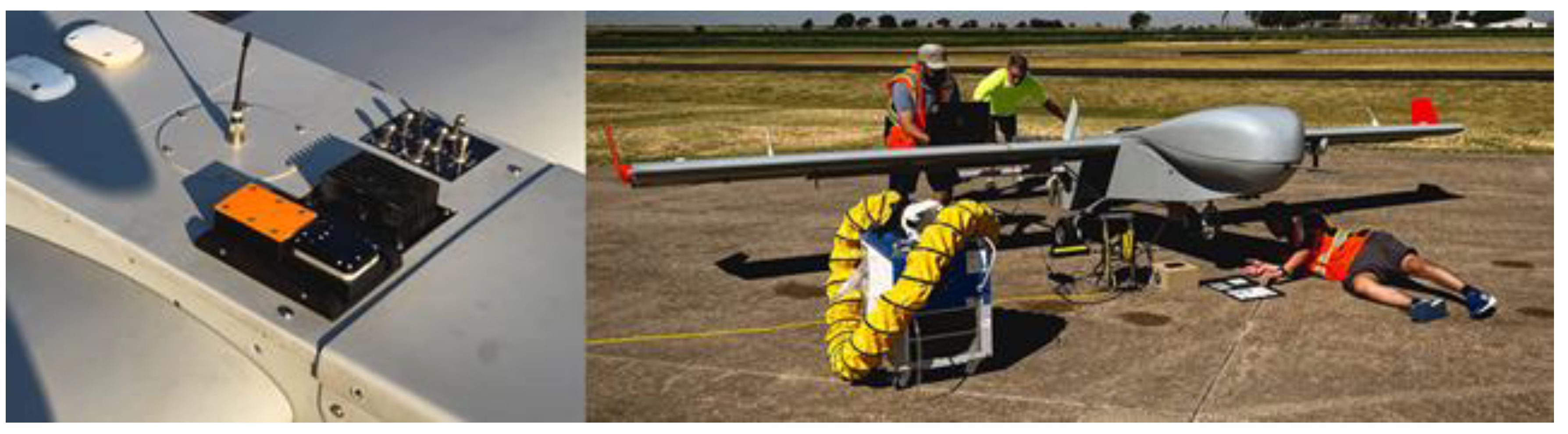
Figure 2.
Top, waypoint map of a sequentially flown imaging flight plan. The turn around points doubled data collection time. An artist’s depiction of the flight pattern is available in Mei et al. 2022. On the bottom is the alternating leg pattern. Because of the wide turning radius, the ArcticShark must jump 6 legs to make the turns. The newer flight plan is faster and more efficient to fly.
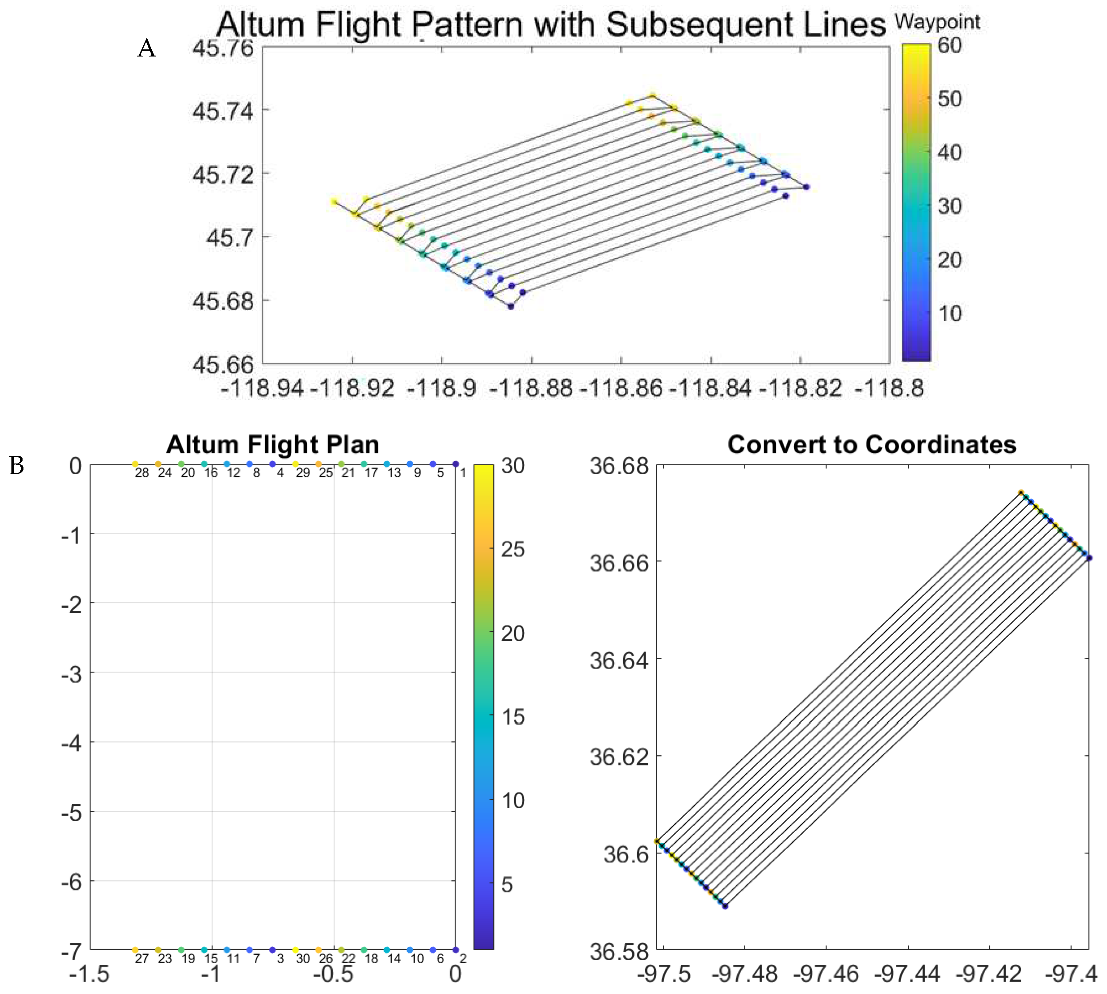
Figure 4.
Apparent reflectance of calibration tarps across the spectral bands (shown as dots) of the Micasense sensor. Solid lines represent published reflectance values. Dashed lines represent pixel values of reflectance images at different altitudes.
Figure 4.
Apparent reflectance of calibration tarps across the spectral bands (shown as dots) of the Micasense sensor. Solid lines represent published reflectance values. Dashed lines represent pixel values of reflectance images at different altitudes.
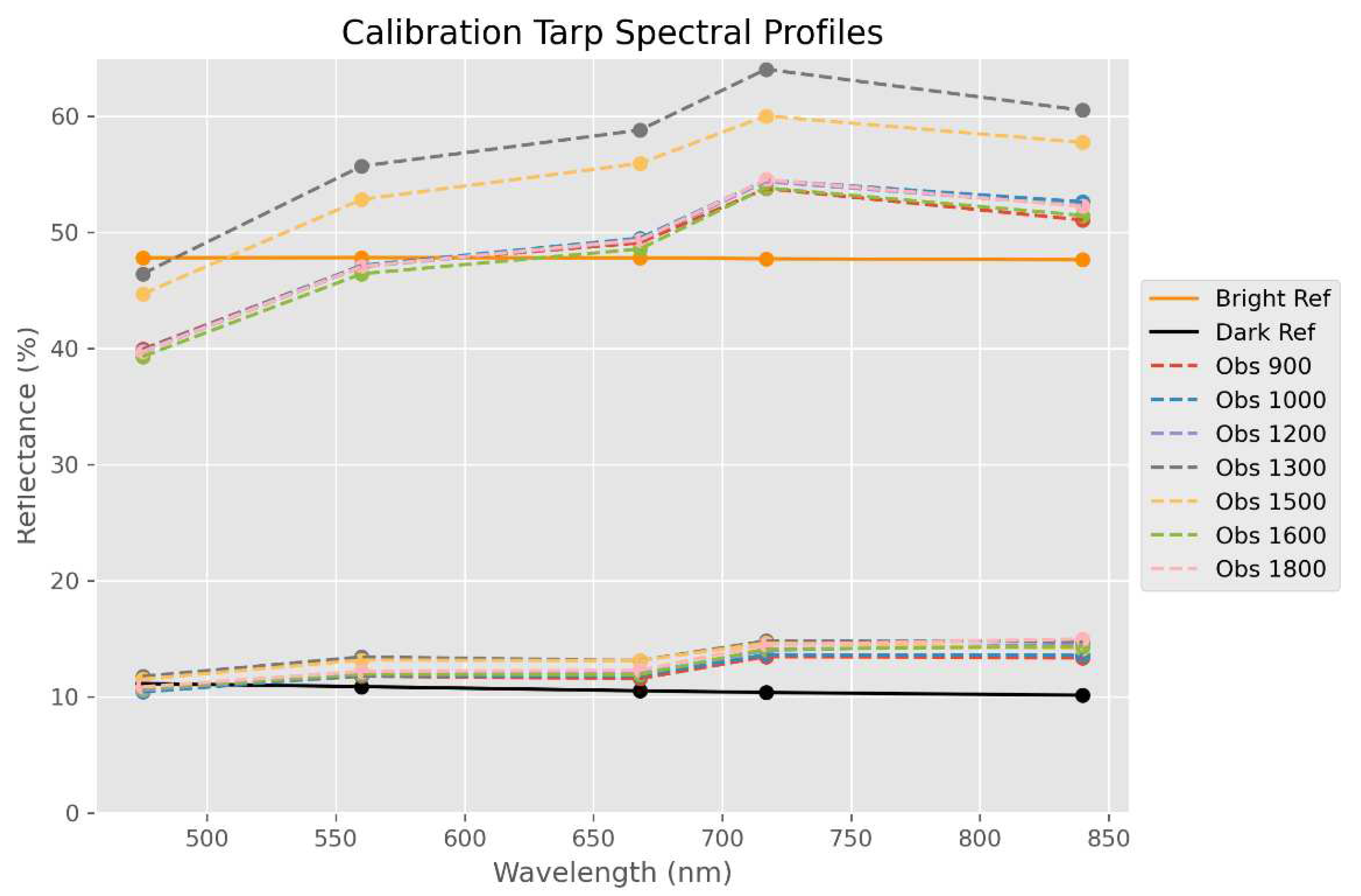
Figure 6.
Left (A,C) bias maps comparing the Altum thermal imagery with the IRT at two different altitudes using the subsequent line flight plan shown in Figure 2 left. Right (B,D), scatter plots of the same comparison points. The two top plots show data from 900 m MSL (520 m AGL), the bottom two plots show data from 1740 m MSL (1360 m AGL).
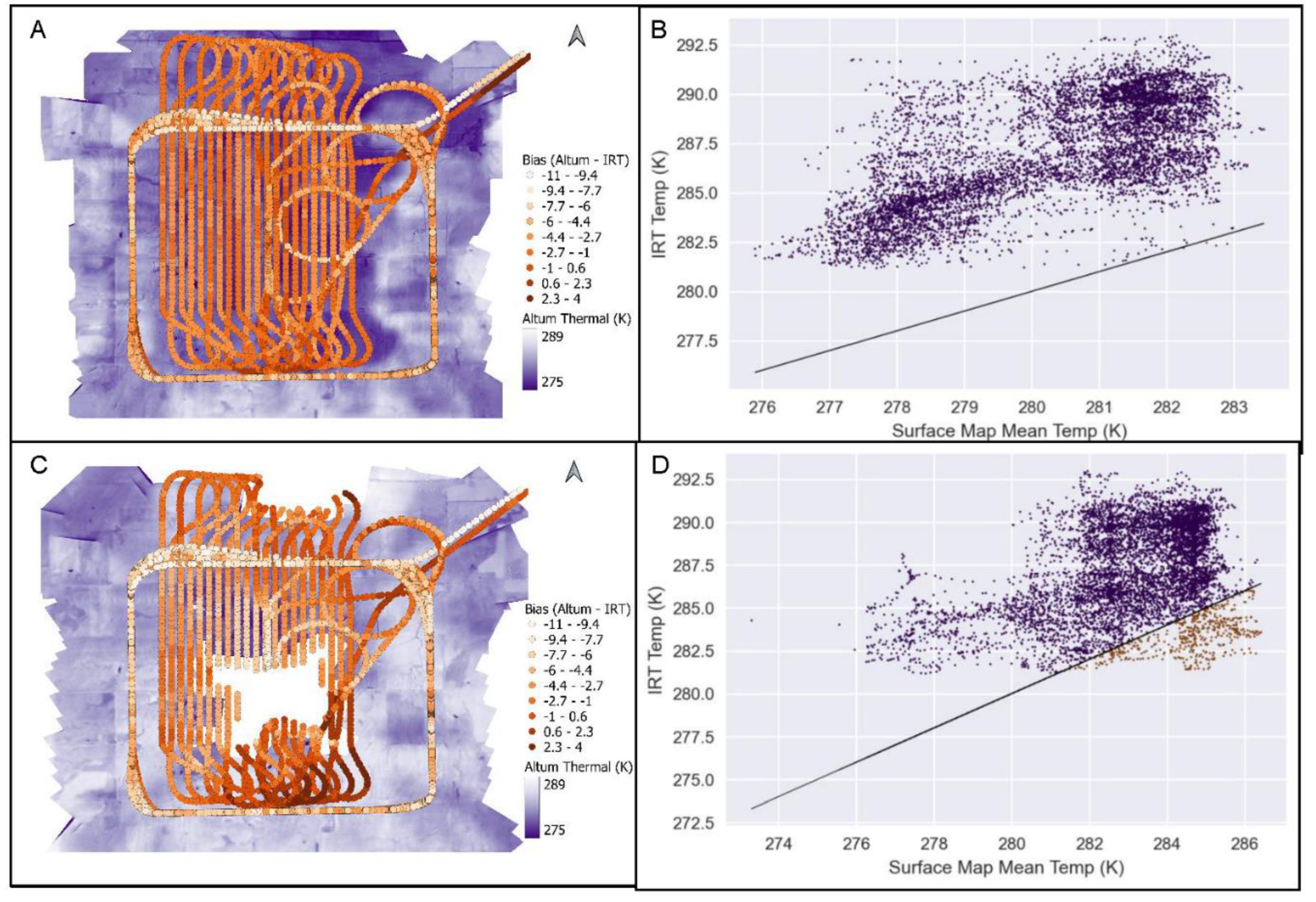
Figure 8.
Sample imagery captured at 820 m AGL with true color on left and calculated normalized difference vegetative index (NDVI) on right.
Figure 8.
Sample imagery captured at 820 m AGL with true color on left and calculated normalized difference vegetative index (NDVI) on right.
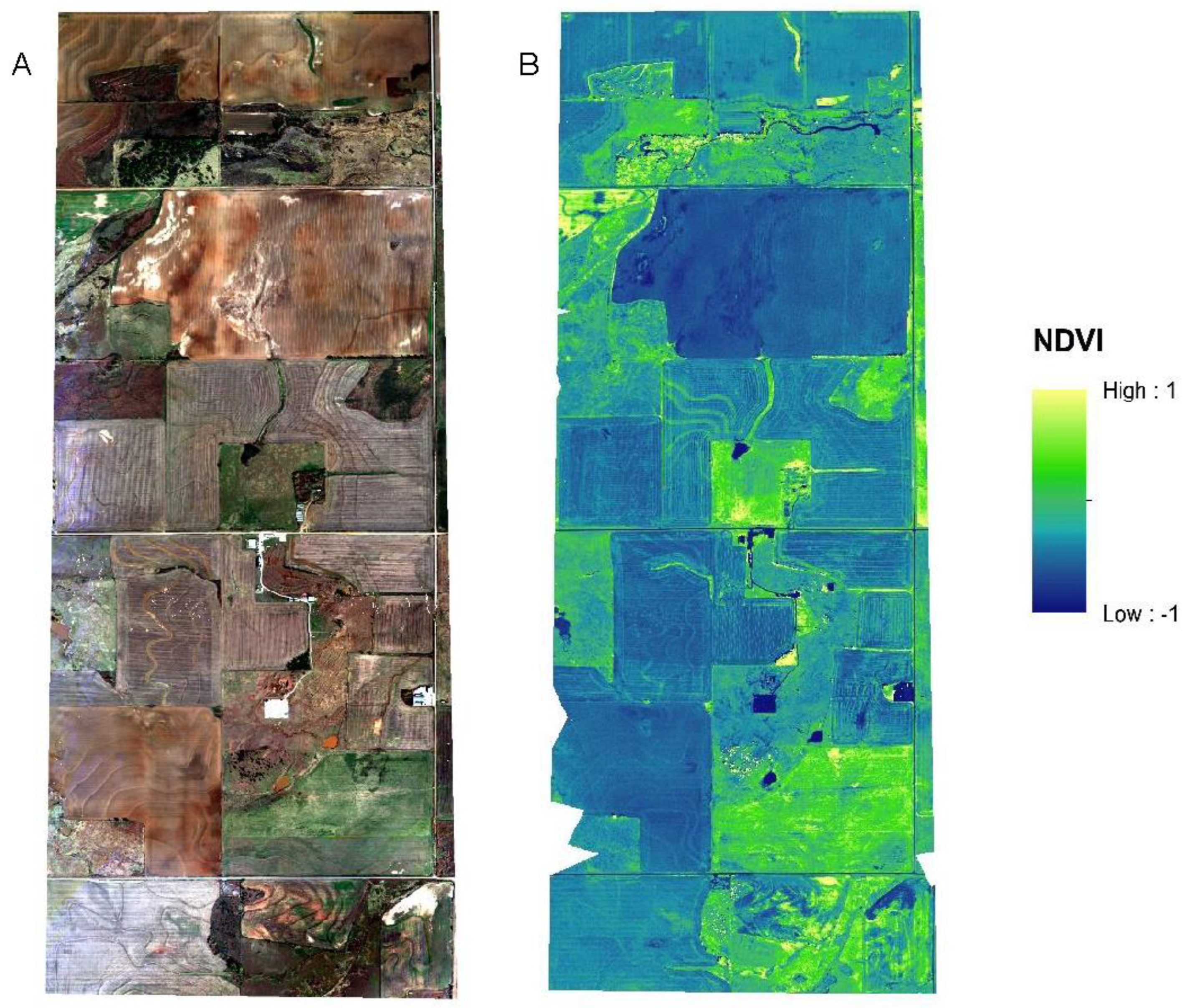
Table 3.
Center and width of the spectral bands recorded by the Altum by MicaSense.
| Name | Center | Bandwidth |
|---|---|---|
| Blue | 475 nm | 32 nm |
| Green | 560 nm | 27 nm |
| Red | 668 nm | 14 nm |
| Red edge | 717 nm | 12 nm |
| Near infrared | 842 nm | 57 nm |
| Thermal | 11,000 nm | 6000 nm |
Disclaimer/Publisher’s Note: The statements, opinions and data contained in all publications are solely those of the individual author(s) and contributor(s) and not of MDPI and/or the editor(s). MDPI and/or the editor(s) disclaim responsibility for any injury to people or property resulting from any ideas, methods, instructions or products referred to in the content. |
© 2023 by the authors. Licensee MDPI, Basel, Switzerland. This article is an open access article distributed under the terms and conditions of the Creative Commons Attribution (CC BY) license (http://creativecommons.org/licenses/by/4.0/).
Copyright: This open access article is published under a Creative Commons CC BY 4.0 license, which permit the free download, distribution, and reuse, provided that the author and preprint are cited in any reuse.


