
Submitted:
07 August 2025
Posted:
11 August 2025
You are already at the latest version
Abstract
Different strategies to include structural mechanical aspects in the design process of hydraulic machines are compared. Therefore, an axial turbine’s runner blade is optimized using evolutionary algorithm. Four different setups with a scalar objective function are investigated. In the first two setups, structural mechanical aspects are added to the optimization process as a constraint, once with a penalty term and once with a modified selection operator. If structural mechanical aspects are considered as a constraint, the risk of a premature convergence increases. For this reason, additionally, two setups including the minimization of the maximum stress as an objective within a scalar objective function are analyzed. Furthermore, a multi-objective optimization with resolution of the Pareto front is done. The differences in the results regarding fitness between the setups using a scalar objective function are small. However, the best result is found for a setup where the minimization of the stress is added as an objective. This demonstrates the risk of a premature convergence involved with constraint handling strategies. The worst result is found for the multi-objective optimization with resolution of the Pareto front, most likely due to a less directed search.
Keywords:
multidisciplinary design optimization
; evolutionary algorithm
; island model
; hydraulic turbine
1. Introduction
The optimization of a hydraulic machine requires the consideration of different objectives like maximizing the efficiency or minimizing the cavitation volume. In addition, there are also constraints like the preservation of the design head. Besides the fluid mechanical aspects, the simultaneous consideration of structural mechanics in the optimization process is important. The reason for this are possible conflicting requirements between the two disciplines regarding certain parameters of a hydraulic machine, such as for example the blade thickness.
The different objectives and constraints lead to a multidisciplinary and multi-objective optimization. There exist two main approaches for multi-objective optimization. The first one is the use of some kind of scalarization to transfer the multi-objective problem into a single-objective, for example by applying the weighted sum approach. In the second approach, a multi-objective algorithm is used to resolute the Pareto front [1]. Furthermore, the compliance of a permissible stress is achieved by adding structural mechanical aspects as a constraint to the optimization problem or by including the minimization of the stresses as an objective. Examples for the different methods to perform a multidisciplinary and multi-objective optimization of a turbomachinery using evolutionary algorithm is found in literature. Luo et al. [2], Song et al. [3], Joly et al. [4], Chirkov et al. [5], Song et al. [6], Li et al. [7], Sen-chun et al. [8], Zhang and Zangeneh [9] and Thandayutham and Samad [10] optimized a turbomachinery with a multi-objective algorithm and the minimization of the maximum stress as an objective. A multi-objective optimization with resolution of the Pareto front considering structural mechanical aspects as a constraint was performed by Lian and Liou [11], Siller et al. [12], Joly et al. [13], Teichel et al. [14], Deng et al. [15] and Lachenmaier et al. [16]. Moreover, there are examples of turbomachinery optimizations done with a scalar objective function and structural mechanics as a constraint [17,18,19,20,21]. However, the focus of the aforementioned works was not on the method of incorporating structural mechanical aspects into the optimization process. Therefore, no comparison of different approaches was created.
The aim of this work is to compare different strategies widely used in the field of turbomachinery to integrate structural mechanical aspects in the optimization process using evolutionary algorithms. This is significant as such a systematic comparison is missing in the literature and results from test functions may not always be transferable to real world problems. Therefore, the pros and cons of different setups used for the optimization of an axial turbine’s runner blade are discussed. The optimization of only a runner blade reduces the numerical effort compared to an entire hydraulic machine, but is realistic enough to achieve reliable results. In the first two setups, a scalar objective function is used including the maintenance of a permissible stress as a constraint, once with a static penalty term and once with a modified selection operator as suggested in [22]. For the consideration of structural mechanics as a constraint, individuals who are infeasible must be severely penalized. This could lead to a situation where an individual fulfilling the permissible stress early in the optimization process dominates infeasible individuals regardless of its other attributes. The feasible individual is then preferably selected for the next parent generation, which can result in an unfavorable reduction in the diversity of certain parameters that are essential for the fluid mechanical properties of the turbine. As a consequence, finding the global minimum gets impossible and premature convergence near the feasible solution occurs. For this reason, additionally, the possibility to include the minimization of the maximum von Mises stress as an objective is investigated, once within a scalar objective function and once via a multi-objective optimization with resolution of the Pareto front.
2. Design Tool
The design of the machines in this contribution is done with design tool Object-Oriented (dtOO) [23,24]. It is written in C++ and provides an interface to Python. Figure 1 gives an overview of the framework. The core of the design system is visualized as the black framed rectangle dtOO. Additionally, the used and most important third party libraries are connected to the box and labeled in vertical direction.
Open Field Operation and Manipulation (OpenFOAM) is used for the simulation of the flow fields. Besides the well-known turbomachinery applications, OpenFOAM is also an open-source and in addition a license-free tool. In order to optimize in parallel with a large number of subprocesses, all dependent libraries within the framework have to be license-free as well. All Computer Aided Design (CAD) functionalities are provided by the occ library. It supports a wide range of CAD functions including import and export. The design framework uses the OpenCASCADE Community Edition (oce) including the pythonocc Python binding. The hybrid meshing procedure is done by using GNU Mesh (GMSH) and, additionally, self-adapted meshing operators to create prismatic layers [25]. During the geometry generation process as well as during the meshing procedure points have to be created on edges, faces and within regions. This task sometimes requires a mapping between a cartesian point and its corresponding point on a geometrical entity. The reparameterization is mostly an iterative procedure and, therefore, performed by minimization techniques provided by the library Cern ROOT (root) [26].
On the left side of Figure 1 an exemplary Python script is shown. The framework implements the Python binding by using Simplified Wrapper and Interface Generator (SWIG) and, therefore, provides counter parts of the C++ classes. Typically, the user then creates the problem definition within self-created Python classes. Then, it is automatically optimized by an appropriate algorithm. On the left bottom side the Pythons’ main dependencies for a typical problem description is shown, too. These external packages have to ensure unique file access for reading and writing (oslo.concurrency) as well as creating subprocesses within the parallel optimization (subprocess). In this contribution a parallel optimization technique based on the island model is used. The Python package pygmo [27] provides an already implemented concept with a lot of optimization algorithms including single- and multi-objective optimization algorithms. As already mentioned all flow field simulations are performed with OpenFOAM. Therefore, swak4Foam is used to support the automated candidates’ evaluations. This task involves the assignment of a fitness value to every candidate.
2.1. Code Structure
The dtOO framework consists of abstract classes to define interfaces for the main classes acting within the framework. Mainly, these are the classes constValue, analyticFunction, analyticGeometry, boundedVolume, dtCase and dtPlugin.
Each geometry’s degree of freedom (DOF) or parameter is represented as an instance of constValue. It provides main functionalities to get, manipulate and store a parameter. By using an observer design pattern [28] all objects are observed in such a way that: if the internal state (the value itself) of one parameter changes, also the overall state label is adjusted. This implements a simple storing mechanism. From a designer’s point of view this mechanism prevents unwanted and unsaved DOFs’ changes.
Many properties of a hydraulic machine do have a distribution over a certain parameter and are, in that sense, a function. As an example, the blade’s inlet angle varies over the spanwise coordinate. Such a function is implemented by an instance of analyticFunction. Within the framework different function types are implemented, e.g. a function being an instance of scaOneD maps from a one dimensional (OneD) input to a one dimensional (sca) output space and an instance of vec2dThreeD maps from a three dimensional (ThreeD) input to a two dimensional (vec2d) output space. All subclasses of analyticFunction provide functions to request function values including derivatives.
Finally, a parameterized hydraulic machine is created and each necessary geometry is represented as an instance of analyticGeometry. Similar to the distinction of the input and output space for analyticFunction the input space of an analyticGeometry varies, too. It means that an edge, face or region is represented by a one, a two or a three dimensional input space, respectively. A geometry always has a three dimensional output space and is typically visualized within ParaVIEW and exported to a CAD file. As an example a map3dTo3d is a region within the framework and, hence, maps from three (3d) to three (3d) dimensions.
A region that can be meshed is implemented as subclass of boundedVolume. As already mentioned the framework uses GMSH as underlying library. Therefore, the bidirectional geometry structure of GMSH [29] is used also within boundedVolume. Due to the complexity of the meshing process, this part of the source code uses observer and builder patterns [28] for clear and extension-friendly structure. Hence, a boundedVolume typically contains multiple map3dTo3d objects, the topological mesh information and the desired mesh operators.
The class dtCase implements necessary functions for setting up a simulation case. Currently, OpenFOAM is connected directly via linking to its libraries and, therefore, enabling an easy setup of the simulation cases.
In order to have a powerful way to implement user-defined extensions without recompiling the complete framework, a simple plugin concept is provided via dtPlugin. An extension, e.g. a new CAD writer can easily be implemented with this concept.
2.2. Python Interface
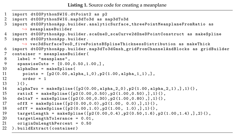
As an example the creation of a meanplane is shown in Listing 1. The import commands import specific parts of the framework (line 1 and 2) and the builders to create the desired geometries (lines 3-6). Line 1 directly import the class dtPoint2 of the framework. According to Figure 1 the class is ported to Python by using SWIG. Classes of the dtOOPythonApp.builder package are designed according to a builder pattern to support the creation of a hydraulic machine. The classes are written in Python and also belong to the dtOO framework, see elliptic shapes in Figure 1. The package dtOOPythonApp.builder provides different builders that create all necessary parts of a hydraulic machine. If a class of the package is not well suited for a designers’ needs, it can easily be extended or, if necessary, a new class can be coded. Each builder can create objects of any type such as constValue, analyticFunction, analyticGeometry, boundedVolume, dtCase and dtPlugin. In order to access the different objects, each builder uses the label argument provided in line 8 to uniquely identify all created objects.
The first builder imported as meanplaneBuilder creates a meanplane that has several DOFs. Adjusting the input argument spanwiseCuts in line 9 changes the number of cuts in radial direction. The argument alphaOne in line 10 defines the inlet angle of the meanplane as a function of the spanwise direction. Therefore, the definition of the function starts by giving a desired number of control points in line 11. A two dimensional point p2 gives the spanwise position and the angle at its first and second coordinate, respectively. The builder makeSpline then creates a B-Spline with given points (line 11) and order (line 12) by calling the ()-operator in line 13. In the same way the other input arguments between line 14 and 19 are defined.
Figure 2 gives a visual definition of the DOFs. Arguments alphaOne, alphaTwo, ratioX, deltaY, offX and offY correspond to symbol , , r, , and , respectively. Increasing parameter r shifts the gray point of top left shown control polygon along gray dashed line to the bottom-right empty gray point. Decreasing the parameter shifts the point in opposite direction. If the parameter is 0 or 1 the mean line’s shape corresponds to the gray dashed lines having an angle of, respectively, or on both sides. Additionally, the mathematical expression of is given in the figure. It is clear that if r assumes extreme values, the meanline does not preserve inlet and outlet angle.
Argument targetLength in line 19 corresponds to the unwound length of the mean line (top right) in Figure 2. It is clear that the parameterization is redundant, because if all three control points (black and grey dots of top figures) of the meanline have defined positions the unwound length is defined, too. But from a designer’s perspective a defined mean line is simply scaled afterwards, preserving its angles and curvatures.
Argument targetLengthTolerance in line 20 is a precision parameter, because the unwound length is iteratively achieved. The last argument originOnLengthPercent shifts then the origin of the two dimensional coordinate system to the unwound length in percent starting from the first control point. A value of means that the origin lies exactly at of the unwound mean line length. This corresponds approximately to the intersection point between the fifth mean line’s normal and the mean line itself. It is only an approximation, because the shown normals are positioned at equidistant parameter and not unwound length values. Again from a designer’s perspective, this parameter enables the creation of a blade that is suspended in the center.
The thickness distribution is modulated to the mean line. As shown in Figure 2, at distinct positions of the mean line (grey digits from 0 to 10) an orthogonal vector is calculated and the thickness is added in this direction.
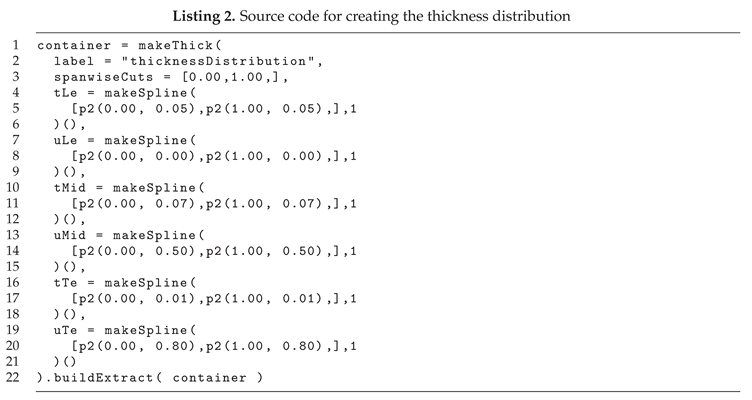
Listing 2 gives the source code for the generation of the thickness distribution schematically shown at the bottom of Figure 2. The builder makeThick is imported in Listing 1 in line 5. Its arguments between lines 2 and 21 of Listing 2 are in line with the previous described builder. In that sense, the attributes label and spanwiseCuts are used again. Additionally, the definition of the thickness is again a function versus the spanwise coordinate and, therefore, functions are created using again the object makeSpline. At the bottom of Figure 2, an exemplary thickness function at a specific spanwise coordinate is presented. The shape of the function is controlled by the coordinates of the three control points, namely their coordinates , , and . At each entry in spanwiseCuts, a B-Spline consisting of five control points is created. All of these splines are then connected to form a surface that defines the thickness of the blade.
After defining all parts of the hydraulic machine, the designer creates the computational grid with the builder imported as gridBuilder in line 6 of Listing 1. Listing 3 gives the arguments of the gridBuilder from line 12 to 34. Figure 3 shows a three dimensional view of the machine including boundary patches with labels and mesh blocks. In order to create such a hybrid mesh that consists of structured mesh blocks, visualized as light grey wireframe, and unstructured mesh elements in the remaining channel, visualized as dark grey wireframe, the builder needs topological information about the structure.
At first, the mesh blocks have to be extracted in line 3 by accessing them via a wildcard to include them in a separate list blocks in line 4. Afterwards, the couplingFaces list of line 5 is filled in lines 8 to 10 with all faces that couple the hexahedral with the tetrahedral mesh part. Line 9 extracts the coupling face from a mesh block by getting a segment with a constant percentage in the third parameter direction.
The visualization in Figure 3 also indicates the parameter dimension and direction with a local frame of reference for each geometry. For the dark gray channel the frame of reference is located on the left surface. According to the figure, the three small lines indicate the third parameter dimension pointing from hub to shroud. A map3dTo3d is a subclass of analyticGeometry and, therefore, a cast operation in line 7 of Listing 3 is mandatory. The arguments channel, blocks, blade and couplingFaces define the topology of the mesh. Additionally, the arguments channelInletOutletDir and channelHubShroudDir define the parameter direction of specific directions. Those topological information is important to correctly label the patches within the grid. All other arguments nBoundaryLayers, nElementsSpanwise and nElementsNormal or firstElementSizeHubToShroud and firstElementSizeNormalBlade or bladeHubElementSize and bladeHubElementScale define the number of elements, their distribution or the first elements sizes located at specific faces (typically walls), respectively.
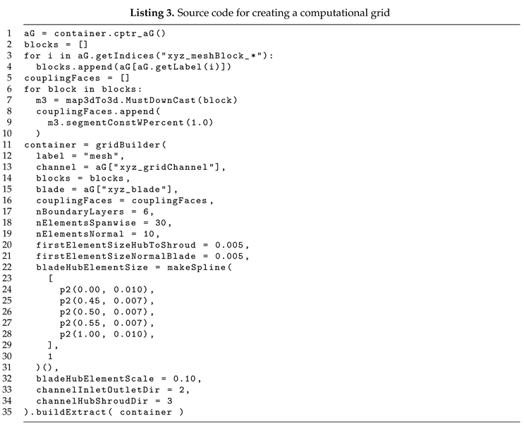
It is evident that the argument bladeHubElementSize defined in lines 22 to 31 is a function that specifies the element size in relation to the unwounded blade length at the hub. Again, a first order B-Spline is created using the makeSpline builder. The gridBuilder object automatically attempts to reach the desired element sizes at the hub as precisely as possible. For each mesh block’s edge lying on the hub, an element size is calculated at each vertex. Additionally, a grading function is applied to this edge to have a smooth transition between the start and end vertex.
3. Models
The numerical setup for the Computational Fluid Dynamics (CFD) and Computational Structural Mechanics (CSM) are introduced in this section. Furthermore, the optimization setups are described. For the parameterization of the machine the previously described model is used. The mean line represented as a B-spline is parameterized with six (, , targetLength, , and r) DOFs. The modulated thickness distribution of the mean line has four (, , and ) DOFs. The mean line as well as the thickness distribution is defined at hub, mid-span and shroud leading to a total of 30 DOFs describing the runner blade.
3.1. Numerical Setup
The geometry used for the optimization is schematically depicted in Figure 3 and consists of a runner channel with a hub radius of 0.5 m and a shroud radius of 1.9 m. For the CSM simulations, a fillet with constant shape is added at the connection between blade and hub. To reduce the numerical effort, static structural mechanical analyses and single-phase steady state flow simulations are performed using OpenFOAM v2206 and the finite element solver CalculiX. Three operating points are simulated during the optimizations whereby the volume flow rates at part load and full load are 0.85 and 1.15 of the volume flow rate at nominal operating point, respectively. The runner rotates with a constant rotational speed of 72 1/min at all operating points. At the inlet, the velocity as well as the turbulent quantities are interpolated from an intake section to ensure realistic inflow conditions. A pressure of 0 Pa is set as outlet boundary condition. As turbulence model, the SST model is used. For the CSM simulations, the forces resulting from the pressure field of the corresponding CFD simulation are set as boundary condition and the hub is clamped on both sides. In addition, centrifugal forces are taken into account. The material for the CSM simulations is steel with a Young’s modulus of 210 000 MPa.
3.2. Optimization Setups
In the following, different optimization setups as well as the parallelization and initialization of the optimization are described. As mentioned above, the optimization algorithms are added to dtOO via the open-source python library pygmo v2.19.0 and the default settings are applied. The algorithms used are differential evolution algorithm (DE) [30] for the optimization setups with a scalar objective function and nondominated sorting genetic algorithm II (NSGA-II) [31] for the multi-objective optimization with resolution of the Pareto front. The reason for selecting these two algorithms is that both are popular in turbomachinery optimization. Because it is difficult to determine whether an optimization is converged, a fixed number of generations is defined for each optimization setup. Thus, the rating of the different setups is based on the ability to achieve good results in a given number of generations. The number of generations is 50 for each optimization with a scalar objective function. Since more evaluations are needed to resolve the Pareto front, the number of generations is increased to 150 for the multi-objective optimization. Furthermore, due to the non-deterministic nature of evolutionary algorithms, three runs per setup are done. This enables a more accurate prediction of the influence of the different setups on the optimization results compared to just a single run, as is the case in most publications dealing with the optimization of turbomachinery. A further increase in the number of runs per setup would increase the reliability of the results, but is not possible because of the high computational effort involved.
3.2.1. Scalar Objective Function
Four different optimization setups using a scalar objective function are analyzed. In the first two setups, structural mechanical aspects are considered as a constraint, once with a static penalty term and once with a modified selection operator according to [22]. In the other setups, the minimization of the maximum von Mises stress is added as an objective. The further designations used for the optimization setups as well as the approach to the structural mechanical aspects are summarized in Table 1.
The optimization goal is to minimize the total fitness which is calculated as the weighted sum of the fitness in the operating points part load , nominal load and full load . Therefore, the optimization problem for setup(DE,C,PT), setup(DE,O) and setup(DE,O,H) can be formulated as:
Minimize
where
The first term in Equation 2 corresponds to the maximization of the efficiency . It follows a function for the minimization of the cavitation volume . At nominal operating point, an additional penalty term is added to the fitness value in case the head H doesn’t match the design head. The last term ensures that the permissible stress is not exceeded.
The functions used for the calculation of the fitness are shown in Figure 4. For the minimization of the cavitation volume, the same e-function is applied for all optimization setups. The value of the function is zero if the cavitation volume is zero and increases with increasing cavitation volume. The feasible region with a maximum von Mises stress below the allowable stress of 80 MPa is represented by the yellow region in the middle part of Figure 4. For setup(DE,C,PT), the value of the function is zero if the maximum von Mises stress is below the allowable stress. Otherwise it increases linear with increasing maximum von Mises stress. The difficulty in this approach is to choose a suitable penalty term. If the slope of the function is set too low, most individuals will be outside of the feasible region at the end of the optimization. In contrast, a too large slope increases the risk of a premature convergence. This possible risk of a premature convergence is reduced by including the minimization of the maximum von Mises stress as an objective to the optimization. The reason for this is that a function with a lower slope can be used and therefore, a non-compliance with the permissible stress is penalized less. If the same slope would be applied, the difference in fitness between two individuals with a maximum von Mises stress above 80 MPa would remain the same. However, analyzing two individuals in the feasible region with comparable fluid mechanical properties, the one with the lower maximum von Mises stress would have the lower fitness in case structural mechanics are considered as objective. This means that the individual is more likely selected for the next parent generation, pushing the optimization towards the feasible region. As a consequence, the slope of the function is decreased. The aim in this approach is to weight all quantities in such a way that the maximum von Mises stress corresponds to the allowable stress at the end of the optimization. For setup(DE,O) and setup(DE,O,H), the same function is applied for the minimization of the maximum von Mises stress. The difference between the two setups is the e-function used for reaching the design head, which is depicted in the lower part of Figure 4. The dotted line corresponds to the design head of 2.4 m and the value of the function increases if the distance to the design head increases. In case structural mechanics are considered as an objective, the weighting of the maximum von Mises stress in the objective function decreases, which increases the weighting of the head. This increased weighting of the head leads to the same potential risk of a premature convergence as described above for the maximum von Mises stress. Therefore, the influence of the head on the objective function is reduced for setup(DE,O,H).
For setup(DE,C,SO), a modified selection operator is used, which has the advantage that no penalty term for non-compliance with the permissible stress has to be specified. The fitness of an individual is calculated according to Equation 1 and 2 and the same functions are used as shown in Figure 4 except the penalty term for the maximum von Mises stress. Instead of the penalty term, the following rules according to [22] are applied for the comparison of two individuals:
- If both individuals are infeasible, the individual with the lower constraint violation is chosen.
- If only one individual is feasible, the feasible individual is chosen.
- If both individuals are feasible, the individual with the lower fitness value is chosen.
3.2.2. Multi-Objective Optimization with Resolution of the Pareto Front
The objectives of the multi-objective optimization with resolution of the Pareto front are the maximization of the efficiency and the minimization of the cavitation volume, both averaged over the three operating points. The highest stresses typically occur under full load due to the highest load on the blade in this operating point. Therefore, the minimization of the maximum von Mises stress at full load is added as third objective. The fourth objective is the minimization of the difference between head at nominal operating point and design head if the deviation from the design head is less than or equal to 20 %. Otherwise, a fitness value is assigned in such a way that each individual outside the feasible region is dominated by any individual within the defined head range. Furthermore, individuals that are closer to the feasible region dominate individuals with higher distances. This treatment of the head is intended to prevent the optimization algorithm exploring the entire head range and thus reduce the optimization effort. The optimization problem is formulated as follows:
Minimize
subject to
3.2.3. Parallelization and Initialization
The optimizations are parallelized using the island model, whereby parallelization is achieved by the number of islands [32]. In Figure 5, a flow chart of the optimization process is exemplarily shown for four islands. All islands are connected to each other which is indicated by the solid lines between the islands on the left side of Figure 5. On each island, the optimization algorithm is executed in serial, which is displayed on the right side of Figure 5. Starting from a parent population, a new child population is created through recombination and, in case of the NSGA-II, mutation. After that, the inner loop of the optimization process, represented by the dashed arrows, is repeated for each individual in the child population in sequence. First, the geometry as well as the CFD mesh are created, followed by the CFD simulations for each operating point. Parallel to the CFD simulations, the CSM mesh is created. After the CFD simulations and the mesh generation finished, the pressure field is interpolated to the CSM mesh and the CSM simulations are performed. The last step in the inner loop is the evaluation, where the fitness is calculated for each individual according to the results of the CFD and CSM simulations. Once the evaluation is completed, the next parent generation is chosen using the selection operator. Before recombination, migration from one randomly picked island occurs. The worst individual on the current island is replaced by the best individual of the selected island. For migration, the migration strategy implemented in pygmo is used which is slightly adapted in a way that migration only occurs if the migration candidate is not already present in the current island population. The migration for the optimization setups with a scalar objective function is fitness based, except setup(DE,C,SO) where the individuals are ranked using the modified selection operator. In the multi-objective optimization with resolution of the Pareto front, individuals are ranked according to [31]. After migration, one generation is completed and the optimization loop starts again.
In this work, the number of islands is set to 20 with a population size of ten on each island for the setups with a scalar objective function. Since the NSGA-II algorithm requires a population size to be a multiple of four, it is set to twelve for the multi-objective optimization with resolution of the Pareto front. The start population is selected from a Latin hypercube sample [33,34] with a size of 1000. The sampling is done with the open-source python library SALib [35,36]. To ensure a homogeneous subpopulation on each island while having diverse ones throughout the archipelago, the sample is clustered with the k-means method [37] using the open-source python library scikit-learn [38]. This corresponds to the idea of the island model of having subpopulations which are placed at different areas of the fitness landscape. The start population is the same for all optimization setups using a scalar objective function. For the multi-objective optimization with resolution of the Pareto front a different start population is taken due to the different population size.
4. Results
In order to compare the different optimization setups, it is assumed that the lower the fitness according to setup(DE,C,PT), the better an individual fits the required characteristics of the turbine. Therefore, the fitness is recalculated similar to setup(DE,C,PT) for each individual after the optimization (Figure 6). The markers, Figure 6 left, correspond to the total mean fitness value of each setup. It is calculated by first averaging the fitness of the ten best individuals for each of the three runs per setup. The total mean fitness value then corresponds to the mean value of these averaged fitness values. Due to the limited number of runs per optimization setup, there is an uncertainty in the calculation of the total mean fitness value. The confidence interval is determined by calculating the standard error of the mean (SEM). The SEM is estimated with the sample standard deviation between the averaged fitness values of each run and the number of runs per setup r as:
Because the SEM is estimated with the sample standard deviation, the means are no longer normally distributed but t-distributed [39]. Therefore, the 95 % confidence interval has to be calculated using the 0.975 quantile of the t-distribution. Taking into account the number of runs per setup, the total mean fitness value lies with a probability of 95 % between . This 95 % confidence interval is represented by the bars in Figure 6, whereby a larger bar indicates a wider spread between the individual runs. Furthermore, for a better understanding of the differences in fitness, the total mean fitness value for each setup is expressed as an equivalent efficiency in the right part of Figure 6.
The lowest total mean fitness value is observed for setup(DE,O,H), which also has a small confidence interval and therefore a low spread between the three runs. It follows in this order setup(DE,C,PT), setup(DE,O), setup(DE,C,SO) and setup(NSGA-II). The results of the total mean fitness value for the optimization setups using a scalar objective function are quite similar. The difference between the setup with the lowest and the setup with the highest total mean fitness value would correspond to a variance in efficiency of 0.74 %. Hence, all of these setups seem to be suitable for the optimization problem. In addition, all setups using a scalar objective function have an overlapping confidence interval. This means, the observed differences could also be a random result caused by the limited number of runs per optimization setup. Nevertheless, the good performance of setup(DE,O,H) indicates a risk of a premature convergence if the penalty for a constraint violation is high. Compared to the results for the setups with a scalar objective function, the performance of setup(NSGA-II) is poor. Despite the fact that the numerical effort is approximately 3.6 times as high, the total mean fitness value would correspond to an efficiency which is 5,33 % lower compared to setup(de,O,H).
Although the differences in terms of fitness between the setups using a scalar objective function are small, interesting variations are found in the evolution of the optimizations. Furthermore, another optimization problem could lead to a more significant effect of premature convergence. Therefore, it still seems worthwhile to discuss the reasons for the observed differences in more detail. This as well as an analysis of the multi-objective optimization with resolution of the Pareto front are presented in the following.
4.1. Scalar Objective Function
In Figure 7, the evolution over the generations for the maximum von Mises stress at full load, the head at nominal load and the averaged efficiency for setup(DE,C,PT), setup(DE,O) and setup(DE,O,H) is presented. Displayed is the mean value of all individuals within one generation averaged over the three runs per setup.
For setup(DE,C,PT), the maximum von Mises stress decreases most rapidly over the number of generations. After ten generations, the average maximum von Mises stress is already below 100 MPa. In contrast, the maximum von Mises stress decreases more slowly for setup(DE,O) and setup(DE,O,H), as expected. Therefore, the risk of a premature convergence is reduced. The slightly greater drop visible for setup(DE,O,H) is caused due to the different function used for the head. Since a deviation from the design head is lower penalized in this setup, the weighting of the maximum von Mises stress in the scalar objective function increases.
Despite the slower decrease of the maximum von Mises stress for setup(DE,O), the results do not improve in terms of fitness compared to setup(DE,C,PT). The reason for this seems to be the evolution of the head versus the number of generations. The decreased weighting of the maximum von Mises stress in the objective function leads to an increased weighting of the head. Hence the head at nominal operating point increases more rapidly which again increases the risk of a premature convergence. Compared to this, the increase of the head for setup(DE,O,H) at the beginning of the optimization lies in between setup(DE,C,PT) and setup(DE,O). Therefore, the risk of a premature convergence is reduced and setup(DE,O,H) even outperforms setup(DE,C,PT) in terms of fitness. The difference between setup(DE,O) and setup(DE,O,H) is clearly visible when looking at the evolution of the efficiency over the generations. Both setups have a faster increase of the efficiency at the beginning of the optimization compared to setup(DE,C,PT). However, while the efficiency for setup(DE,O) is similar to setup(DE,C,PT) at around generation 25, it continues to be higher for setup(DE,O,H).
The difference in the results between the setups illustrate the risk of a premature convergence if a non-compliance with the constraints is severely penalized. This is true for the design head as the comparison of setup(DE,O) and setup(DE,O,H) shows. Furthermore, since the head increases faster over the generations for setup(DE,O,H) compared to setup(DE,C,PT) at the beginning of the optimization, the reason for the better result regarding fitness for this setup seems to be the lower decrease of the maximum von Mises stress. Therefore, the risk of a premature convergence also applies to the maximum von Mises stress. This does not mean that results similar to setup(DE,O,H) are not possible using a penalty term for the stresses. For this study, only one penalty function is tested. Better results may be achieved by lowering the weighting of the penalty term. Nevertheless, it clearly demonstrates the difficulty of choosing a static penalty term appropriate for the optimization problem.
In Figure 8, the evolution of the CFD fitness over the number of generations is displayed for setup(DE,C,PT) and setup(DE,C,SO). For the calculation of the CFD fitness, only the results for the efficiency, cavitation and head at nominal operating point are taken into account and structural mechanical aspects are not considered. The lines correspond to the best individual found so far regarding CFD fitness, averaged over the three runs per setup. Furthermore, the evolution of the maximum von Mises stress at full load and the head at nominal operating point over the generations is shown in Figure 8. In those cases, the lines correspond to the mean value of all individuals within one generation averaged over the three runs per setup.
In the start population, there are only 25 individuals out of 200 which fulfilling the permissible stress requirement. With the modified selection operator implemented for setup(DE,C,SO), fluid mechanical aspects are only considered if both compared individuals are in the feasible region. This means that at the beginning of the optimization, mainly structural mechanical aspects for setup(DE,C,SO) are improved, which becomes visible in the evolution of the CFD fitness. Until generation 14, there is nearly no improvement for the CFD fitness and therefore no improvement regarding fluid mechanical aspects of the turbine. Furthermore, this leads to a faster decrease of the stresses at the beginning and a lower averaged maximum von Mises stress at the end of the optimization compared to setup(DE,C,PT). After generation 17, the averaged von Mises stress is within or very close to the permissible stress. This indicates that a non-compliance with the permissible stress is harder penalized for setup(DE,C,SO). At the same time, the head at nominal operating point increases slower compared to setup(DE,C,PT) and the averaged head is below the design head at the end of the optimization. The comparison of the results for setup(DE,C,PT), setup(DE,O) and setup(DE,O,H) suggest that such an evolution of the head could be beneficial regarding fitness. This is not the case here, since the fitness values achieved for setup(DE,C,SO) tend to be similar or even worse than those for setup(DE,C,PT). The reason for this could be that at the beginning of the optimization mainly structural mechanical aspects are optimized. This increases the risk of a premature convergence and seems to outweighs a possible advantage due to the evolution of the head.
4.2. Multi-Objective Optimization with Resolution of the Pareto Front
The Pareto fronts obtained for the three runs with the NSGA-II are depicted in Figure 9. All individuals on the Pareto front are represented by the gray markers while the red markers are the best overall 20 individuals from all setups analyzed. Looking at the cavitation volume over efficiency, it is noticeable that there is only a small range around efficiencies of 90 % where the cavitation volume is low. As the efficiency decreases, the cavitation volume increases due to an increasing misaligned flow to the blade. For the maximum von Mises stress, there is a trade-off with the efficiency visible. If the efficiency increases, the maximum von Mises stress tends to increase as well. Starting from an efficiency of around 94 %, no further increase in efficiency is possible without leaving the feasible region.
The overall best individuals are all within a very small range of the Pareto front, which points out the reason for the struggle of the NSGA-II to find individuals of similar fitness compared to the DE. Due to the nature of a multi-objective optimizer, the NSGA-II resolves the Pareto front at positions, which are not of interest for the optimization problem. This problem could be overcome by limiting other quantities like, for example, the maximum von Mises stress in a similar way as the head. However, this also increases the risk of a premature convergence.
Another possible reason for the lower performance of the NSGA-II is the use of the island model for parallelization. Investigations on a simple test function indicate that the island model is not so well suited for optimization with the NSGA-II. The reason for this is most likely that, despite of migration, the optimization process is separated between the islands. Therefore it is possible that different islands resolve similar positions of the Pareto front at the same time, which could lead to a slower convergence of the optimization. Hence, it can not be excluded that better results would be obtained with a master-slave parallelization. Furthermore, the different treatment of the head compared to the optimization setups using a scalar objective function could have an influence on the results. Nevertheless, if the required characteristics of a hydraulic machine are known before optimization, there is no reason to explore the entire objective range.
5. Conclusion and Outlook
The comparison of different strategies to include structural mechanical aspects in the design process of an axial turbine’s runner blade is presented. Fluid mechanical objectives of the optimization are the maximization of the efficiency and minimization of the cavitation volume while preserving the design head at nominal operating point. Four different setups using the DE with a scalar objective function are investigated. In two setups, structural mechanical aspects are added to the optimization process as a constraint, once with a penalty term and once with a different selection operator. In addition, two setups including the minimization of the maximum von Mises stress as an objective within a scalar objective function are analyzed. Furthermore, a multi-objective optimization with the NSGA-II and resolution of the Pareto front is executed. Due to the non-deterministic nature of evolutionary algorithm, each setup is repeated twice.
The difference in the results in terms of fitness for the setups using a scalar objective function are small. Hence, all of these setups seems to be suitable for the optimization problem. Nevertheless, some interesting variance between the setups are found. A comparison of the two setups, where structural mechanical aspects are considered as a constraint, mainly shows an improvement regarding stresses at the beginning of the optimization if the modified selection operator is applied. The reason for this is that in this setup fluid mechanical aspects are only considered if both compared individuals are fulfilling the permissible stress. This could lead to problems when optimizing an entire machine due to the more complex fluid mechanical task. One advantage of the modified selection operator is that no penalty term has to be chosen and the objective function regarding fluid mechanical aspects can be adjusted independent of structural mechanical stress limits. At the same time, this also makes it impossible to adapt the treatment of the constraint according to the optimization problem. The use of a penalty term allows a more flexible adjustment of the treatment of the constraint. One challenge, however, is to find a suitable penalty term. If infeasible individuals are penalized too strong, the risk of a premature convergence increases. On the other hand, a too low weighting leads to a low drift of the optimization towards the feasible region. Furthermore, each adjustment of the objective function regarding fluid mechanical aspects requires a correction of the penalty term.
The risk of a premature convergence is reduced if the minimization of the maximum von Mises stress is added as an objective. This is because the proportion of the stresses in the objective function is reduced, resulting in a slower decrease of the maximum von Mises stress during the optimization. However, the reduced weighting of the stresses leads to an increased weighting of the head which also increases the risk of a premature convergence. Therefore, no better results are obtained if the minimization of the maximum von Mises stress is added as an objective without adjusting the penalty term for non-compliance with the design head. If the penalty term for the head is additionally adjusted, the best overall results regarding fitness are achieved. This demonstrates the risk of a premature convergence if a non-compliance with the constraints is severely penalized. At the same time, it is not excluded that similar results may be obtained with a lower weighted penalty term. Furthermore, finding the right function to minimize the stresses is challenging and may require multiple iterations. The reason for this is the trade-off between increasing the efficiency and decreasing the stresses. This leads to bad results if the best individuals are significantly below the permissible stress at the end of the optimization due to an overweighting of structural mechanical aspects.
Compared to the setups using a scalar objective function, the results regarding the fitness are poor if a multi-objective optimization with resolution of the Pareto front is performed. The main reason for this appears to be a less directed search compared to an optimization using a scalar objective function. Therefore, if the required characteristics of a hydraulic machine are known before optimization, it seems to be more reasonable to carry out an optimization using some kind of scalarization such as a scalar objective function. This may require some iterative adjustments of the objective function. However, due to the higher numerical effort of a multi-objective optimization, it should still be possible to find better individuals in a comparable time. Another possible solution to address the drawbacks identified for NSGA-II is to use a different multi-objective algorithm such as nondominated sorting genetic algorithm III (NSGA-III) [40,41]. With NSGA-III, a preferred region of the Pareto front can be specified using reference points thus allowing a more directed search. Furthermore, the algorithm is designed to provide improvements for optimizations with four or more objectives. Unfortunately, NSGA-III is not available in pygmo which is the main reason why it was not analyzed in this work. However, this must be addressed in future work.
When interpreting the results, it has to be kept in mind that all optimization runs are parallized using the island model. A generalization to a serial optimization is not possible. Furthermore, the results may vary depending on the optimization algorithm used as well as depending on the settings of the respective algorithm. Nevertheless, the results demonstrate the risk of a premature convergence if individuals violating the permissible stress are severely penalized.
One possible approach to reduce the risk of a premature convergence could be the use of different and potentially more complex constraint handling methods such as a dynamic penalty term. Therefore, the investigation of additional methods is a possible next step. Furthermore, in this work migration is fitness based. The use of a more diversity based migration strategy may reduce the risk of a premature convergence and is recommended to investigate. Finally, all studies are supposed to be repeated on an entire hydraulic machine. This may lead to different results due to the more complex fluid mechanical problem.
Author Contributions
Conceptualization, S.F. and A.T.; methodology, S.F. and A.T.; software, S.F. and A.T.; validation, S.F.; formal analysis, S.F.; investigation, S.F.; data curation, S.F.; writing—original draft preparation, S.F. and A.T.; writing—review and editing, S.F., A.T. and S.R.; visualization, S.F. and A.T.; supervision, A.T. and S.R. All authors have read and agreed to the published version of the manuscript.
Funding
This research received no external funding.
Data Availability Statement
The datasets presented in this article are not readily available because the data are part of an ongoing study. Requests to access the datasets should be directed to alexander.tismer@ihs.uni-stuttgart.de. However, the design tool as well as the test case are publicly available in ihs-ustutt/dtOO at https://github.com/ihs-ustutt/dtOO. Besides this, only open-source libraries mentioned in the paper were used, which allows replication of the results.
Acknowledgments
The simulations were performed on the national supercomputer HPE Apollo Hawk at the High Performance Computing Center Stuttgart (HLRS) under the grant number 44196. Preliminary studies are done on the bwUniCluster 2.0. The authors acknowledge support by the state of Baden-Württemberg through bwHPC.
Conflicts of Interest
The authors declare no conflicts of interest.
Abbreviations
The following abbreviations are used in this manuscript:
| CAD | Computer Aided Design |
| CFD | Computational Fluid Dynamics |
| CSM | Computational Structural Mechanics |
| DE | differential evolution algorithms |
| DOF | degree of freedoms |
| dtOO | design tool Object-Orienteds |
| GMSH | GNU Mesh |
| NSGA-II | nondominated sorting genetic algorithm IIs |
| NSGA-III | nondominated sorting genetic algorithm IIIs |
| OpenFOAM | Open Field Operation and Manipulation |
| root | Cern ROOT |
| SEM | standard error of the means |
| SWIG | Simplified Wrapper and Interface Generator |
References
- Cui, Y.; Geng, Z.; Zhu, Q.; Han, Y. Review: Multi-objective optimization methods and application in energy saving. Energy 2017, 125, 681–704. [Google Scholar] [CrossRef]
- Luo, C.; Song, L.; Li, J.; Feng, Z. A Study on Multidisciplinary Optimization of an Axial Compressor Blade Based on Evolutionary Algorithms. J. Turbomach. 2012, 134, 054501. [Google Scholar] [CrossRef]
- Song, L.; Luo, C.; Li, J.; Feng, Z. Automated multi-objective and multidisciplinary design optimization of a transonic turbine stage. Proceedings of the Institution of Mechanical Engineers, Part A: Journal of Power and Energy 2012, 226, 262–276. [Google Scholar] [CrossRef]
- Joly, M.M.; Verstraete, T.; Paniagua, G. Multidisciplinary design optimization of a compact highly loaded fan. Struct. Multidisc. Optim. 2014, 49, 471–483. [Google Scholar] [CrossRef]
- Chirkov, D.V.; Ankudinova, A.S.; Kryukov, A.E.; Cherny, S.G.; Skorospelov, V.A. Multi-objective shape optimization of a hydraulic turbine runner using efficiency, strength and weight criteria. Struct. Multidisc. Optim. 2018, 58, 627–640. [Google Scholar] [CrossRef]
- Song, Y.H.; Guo, P.C.; Sun, L.G.; Zhou, H.T.; Luo, X.Q. Multidisciplinary design optimization on the splitter blade of high head Francis turbine. IOP Conf. Ser.: Earth Environ. Sci. 2018, 163, 012032. [Google Scholar] [CrossRef]
- Li, C.; Wang, J.; Guo, Z.; Song, L.; Li, J. Aero-mechanical multidisciplinary optimization of a high speed centrifugal impeller. Aerosp. Sci. Technol. 2019, 95, 105452. [Google Scholar] [CrossRef]
- Sen-chun, M.; Hong-biao, Z.; Ting-ting, W.; Xiao-hui, W.; Feng-xia, S. Optimal design of blade in pump as turbine based on multidisciplinary feasible method. Sci. Prog. 2020, 103, 0036850420982105. [Google Scholar] [CrossRef]
- Zhang, J.; Zangeneh, M. Multidisciplinary and multi-point optimisation of radial and mixed-inflow turbines for turbochargers using 3D inverse design method. In Proceedings of the 14th International Conference on Turbochargers and Turbocharging; Institution of Mechanical Engineers., Ed., London, UK; 2020; pp. 263–277. [Google Scholar] [CrossRef]
- Thandayutham, K.; Samad, A. Hydrostructural Optimization of a Marine Current Turbine Through Multi-fidelity Numerical Models. Arab. J. Sci. Eng. 2020, 45, 935–952. [Google Scholar] [CrossRef]
- Lian, Y.; Liou, M.S. Aerostructural Optimization of a Transonic Compressor Rotor. J. Propuls. Power 2006, 22, 880–888. [Google Scholar] [CrossRef]
- Siller, U.; Voß, C.; Nicke, E. Automated Multidisciplinary Optimization of a Transonic Axial Compressor. In Proceedings of the 47th AIAA Aerospace Sciences Meeting Including The New Horizons Forum and Aerospace Exposition, Orlando, Florida, USA, January 2009; p. 863. [Google Scholar] [CrossRef]
- Joly, M.M.; Verstraete, T.; Paniagua, G. Integrated multifidelity, multidisciplinary evolutionary design optimization of counterrotating compressors. Integrated Computer-Aided Engineering 2014, 21, 249–261. [Google Scholar] [CrossRef]
- Teichel, S.; Verstraete, T.; Seume, J. Optimized Multidisciplinary Design of a Small Transonic Compressor for Active High-Lift Systems. Int. J. Gas Turbine Propuls. Power Syst. 2017, 9, 19–26. [Google Scholar] [CrossRef]
- Deng, Q.; Shao, S.; Fu, L.; Luan, H.; Feng, Z. An Integrated Design and Optimization Approach for Radial Inflow Turbines—Part II: Multidisciplinary Optimization Design. Appl. Sci. 2018, 8. [Google Scholar] [CrossRef]
- Lachenmaier, N.; Baumgärtner, D.; Schiffer, H.P.; Kech, J. Gradient-Free and Gradient-Based Optimization of a Radial Turbine. Int. J. Turbomach. Propuls. Power. 2020, 5, 14. [Google Scholar] [CrossRef]
- Pierret, S.; Filomeno Coelho, R.; Kato, H. Multidisciplinary and multiple operating points shape optimization of three-dimensional compressor blades. Struct. Multidisc. Optim. 2007, 33, 61–70. [Google Scholar] [CrossRef]
- Verstraete, T.; Alsalihi, Z.; Van den Braembussche, R.A. Multidisciplinary Optimization of a Radial Compressor for Microgas Turbine Applications. J. Turbomach. 2010, 132, 031004. [Google Scholar] [CrossRef]
- Bannikov, D.V.; Yesipov, D.V.; Cherny, S.G.; Chirkov, D.V. Optimization design of hydroturbine rotors according to the efficiency-strength criteria. Thermophys. Aeromech. 2010, 17, 613–620. [Google Scholar] [CrossRef]
- Van den Braembussche, R.A.; Alsalihi, Z.; Verstraete, T.; Matsuo, A.; Ibaraki, S.; Sugimoto, K.; Tomita, I. Multidisciplinary Multipoint Optimization of a Transonic Turbocharger Compressor. In Proceedings of the Proceedings of the ASME Turbo Expo 2012: Turbine Technical Conference and Exposition, Copenhagen, Denmark, June 2012. [CrossRef]
- Aissa, M.H.; Verstraete, T. Metamodel-Assisted Multidisciplinary Design Optimization of a Radial Compressor. Int. J. Turbomach. Propuls. Power 2019, 4, 35. [Google Scholar] [CrossRef]
- Deb, K. An efficient constraint handling method for genetic algorithms. Comput. Methods Appl. Mech. Eng. 2000, 186, 311–338. [Google Scholar] [CrossRef]
- Tismer, A. Entwicklung einer Softwareumgebung zur automatischen Auslegung von hydraulischen Maschinen mit dem Inselmodell. PhD thesis, Universität Stuttgart, Stuttgart, Germany, 2020. Available at https://d-nb.info/1220692778/34.
- Tismer, A. ihs-ustutt/dtOO; 2024. Available at https://github.com/ihs-ustutt/dtOO.
- Tismer, A.; Schlipf, M.; Riedelbauch, S. Sensitivity Study of the Numerical Setup for an Automatic Optimization Procedure for a Hydraulic Machine. In Proceedings of the VII European Congress on Computational Methods in Applied Sciences and Engineering, Crete Island, Greece, June 2016; VII. [Google Scholar] [CrossRef]
- Brun, R.; Rademakers, F.; Canal, P.; Naumann, A.; Couet, O.; Moneta, L.; Vassilev, V.; Linev, S.; Piparo, D.; GANIS, G.; et al. root-project/root: v6.18/02; Zenodo, 2020. [CrossRef]
- Biscani, F.; Izzo, D. A parallel global multiobjective framework for optimization: pagmo. J. Open Source Softw. 2020, 5, 2338. [Google Scholar] [CrossRef]
- Gamma, E.; Helm, R.; Johnson, R.; Vlissides, J.M. Design Patterns: Elements of Reusable Object-Oriented Software, 1 ed.; Addison-Wesley Professional, 1994.
- Geuzaine, C.; Remacle, J.F. Gmsh: A 3-D finite element mesh generator with built-in pre- and post-processing facilities. Int. J. Numer. Methods Eng. 2009, 79, 1309–1331. [Google Scholar] [CrossRef]
- Storn, R.; Price, K. Differential Evolution - A Simple and Efficient Heuristic for global Optimization over Continuous Spaces. J. Glob. Optim. 1997, 11, 341–359. [Google Scholar] [CrossRef]
- Deb, K.; Pratap, A.; Agarwal, S.; Meyarivan, T. A fast and elitist multiobjective genetic algorithm: NSGA-II. IEEE Trans. Evol. Comput. 2002, 6, 182–197. [Google Scholar] [CrossRef]
- Cohoon, J.P.; Hegde, S.U.; Martin, W.N.; Richards, D. Punctuated Equilibria: A Parallel Genetic Algorithm. In Proceedings of the Second International Conference on Genetic Algorithms and Their Application, USA; 1987; pp. 148–154. [Google Scholar]
- McKay, M.D.; Beckman, R.J.; Conover, W.J. A Comparison of Three Methods for Selecting Values of Input Variables in the Analysis of Output from a Computer Code. Technometrics 1979, 21, 239–245. [Google Scholar] [CrossRef]
- Iman, R.L.; Helton, J.C.; Campbell, J.E. An Approach to Sensitivity Analysis of Computer Models: Part I—Introduction, Input Variable Selection and Preliminary Variable Assessment. J. Qual. Technol. 1981, 13, 174–183. [Google Scholar] [CrossRef]
- Herman, J.; Usher, W. SALib: An open-source Python library for Sensitivity Analysis. J. Open Source Softw. 2017, 2. [Google Scholar] [CrossRef]
- Iwanaga, T.; Usher, W.; Herman, J. Toward SALib 2.0: Advancing the accessibility and interpretability of global sensitivity analyses. Socio-Environmental Systems Modelling 2022, 4, 18155. [Google Scholar] [CrossRef]
- MacKay, D.J.C. Information Theory, Inference and Learning Algorithms; Cambridge University Press, 2003.
- Pedregosa, F.; Varoquaux, G.; Gramfort, A.; Michel, V.; Thirion, B.; Grisel, O.; Blondel, M.; Prettenhofer, P.; Weiss, R.; Dubourg, V.; et al. Scikit-learn: Machine Learning in Python. J. Mach. Learn. Res. 2011, 12, 2825–2830. [Google Scholar]
- Janczyk, M.; Pfister, R. Understanding Inferential Statistics: From A for Significance Test to Z for Confidence Interval, 1 ed.; Springer Berlin: Heidelberg, 2023. [Google Scholar] [CrossRef]
- Deb, K.; Jain, H. An Evolutionary Many-Objective Optimization Algorithm Using Reference-Point-Based Nondominated Sorting Approach, Part I: Solving Problems With Box Constraints. IEEE Trans. Evol. Comput. 2014, 18, 577–601. [Google Scholar] [CrossRef]
- Jain, H.; Deb, K. An Evolutionary Many-Objective Optimization Algorithm Using Reference-Point Based Nondominated Sorting Approach, Part II: Handling Constraints and Extending to an Adaptive Approach. IEEE Trans. Evol. Comput. 2014, 18, 602–622. [Google Scholar] [CrossRef]
Figure 1.
Schematic overview of the design framework dtOO; Main dependencies for the C++ and Python code written in vertical and horizontal direction, respectively; Elliptical shapes show the additional Python library for supporting the creation of a hydraulic machine
Figure 1.
Schematic overview of the design framework dtOO; Main dependencies for the C++ and Python code written in vertical and horizontal direction, respectively; Elliptical shapes show the additional Python library for supporting the creation of a hydraulic machine
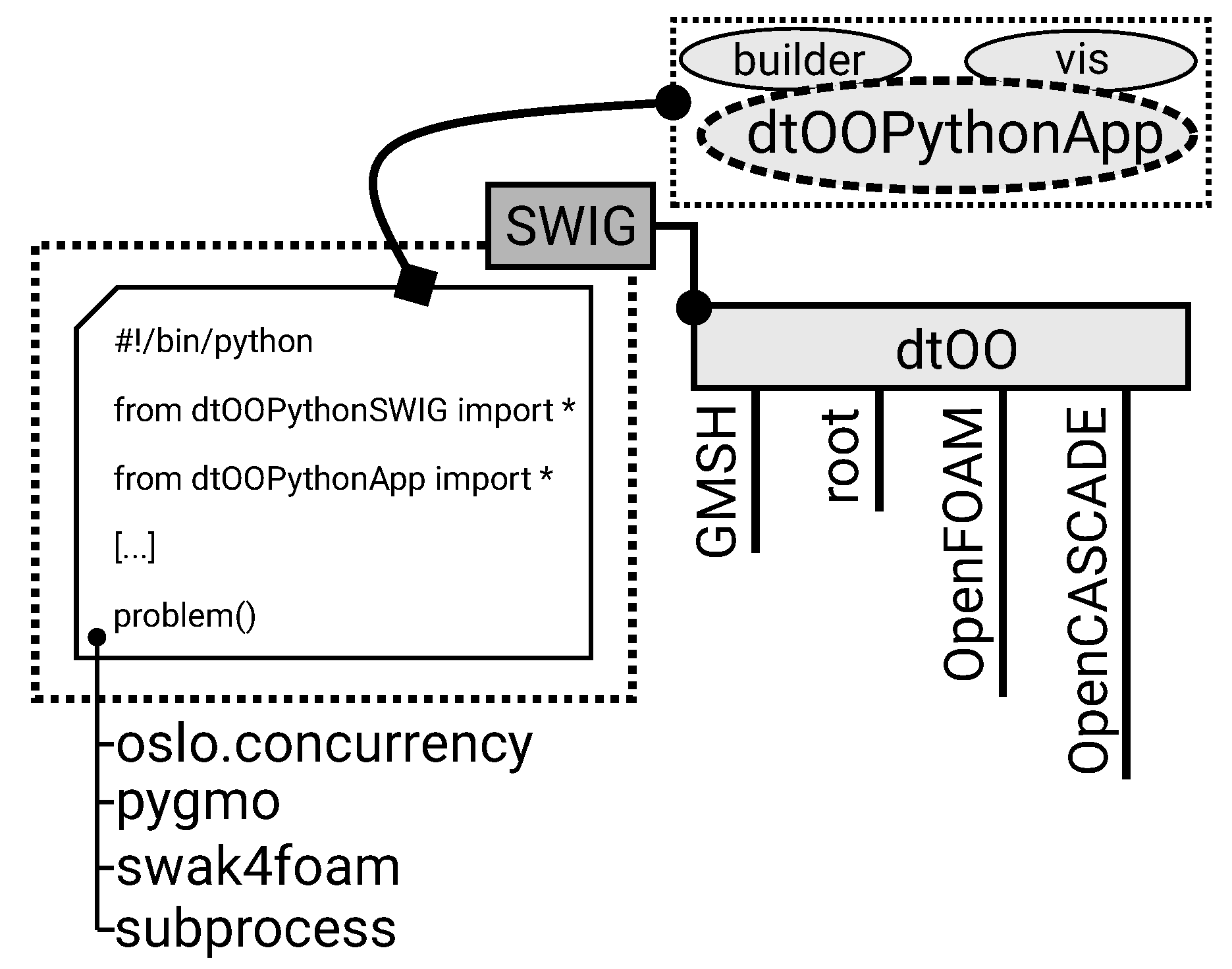
Figure 2.
Parameterization of the runner blade including mean line (top left) and thickness modulation (top right); Thickness distribution (bottom) including its parameterization; DOFs added and labeled as, respectively, black arrows and symbols
Figure 2.
Parameterization of the runner blade including mean line (top left) and thickness modulation (top right); Thickness distribution (bottom) including its parameterization; DOFs added and labeled as, respectively, black arrows and symbols
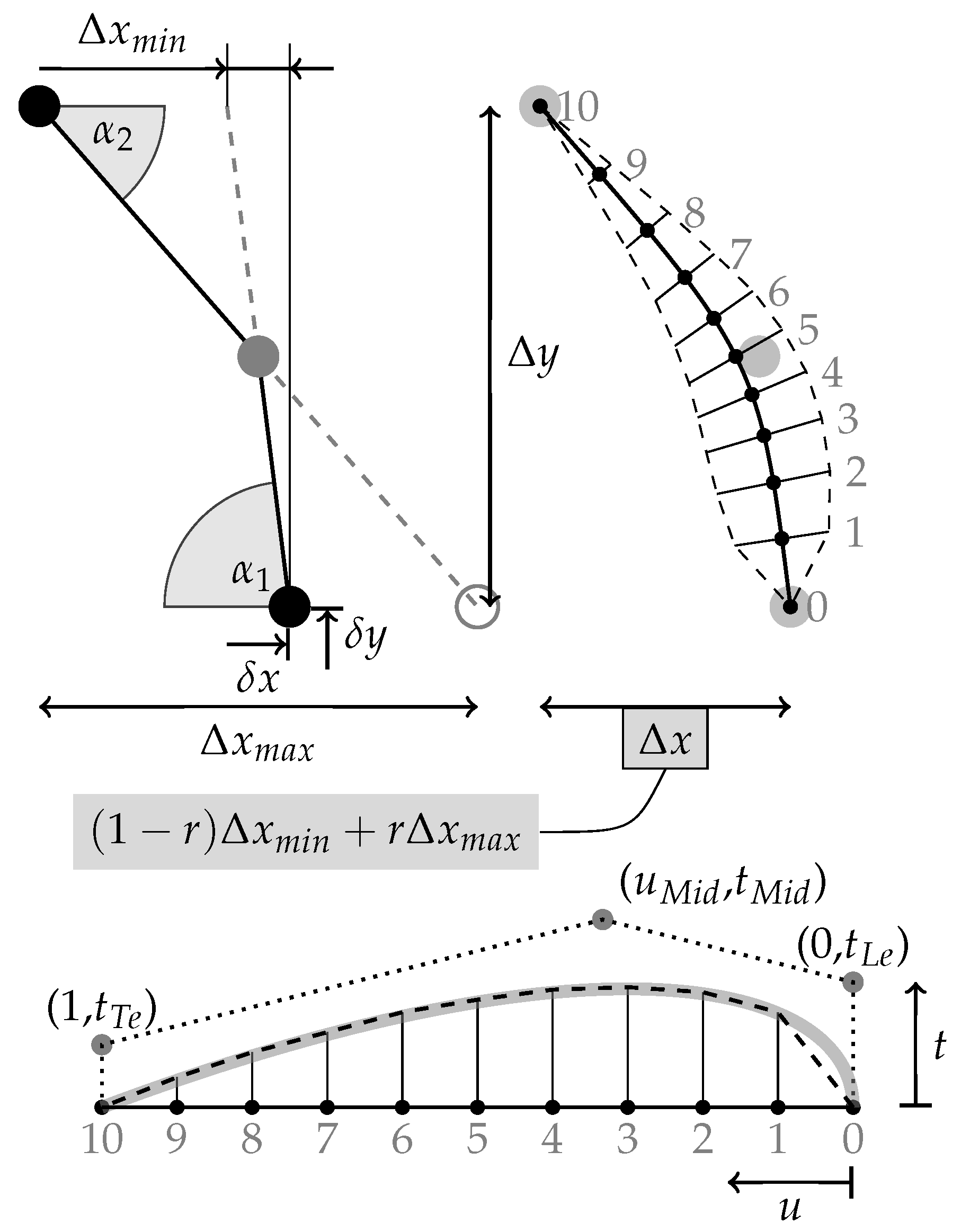
Figure 3.
Axial turbine blade with channel geometry including mesh blocks surrounding the blade; Labels indicated with arrows pointing to corresponding face; Parametric space direction shown as dashed lines
Figure 3.
Axial turbine blade with channel geometry including mesh blocks surrounding the blade; Labels indicated with arrows pointing to corresponding face; Parametric space direction shown as dashed lines
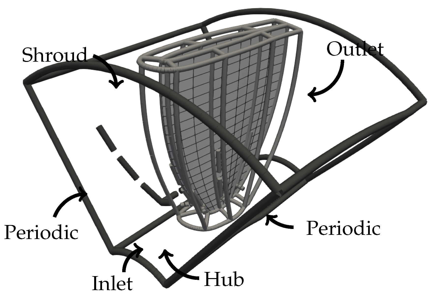
Figure 4.
Functions used for the cavitation volume, the maximum von Mises stress and the head in the scalar objective function
Figure 4.
Functions used for the cavitation volume, the maximum von Mises stress and the head in the scalar objective function
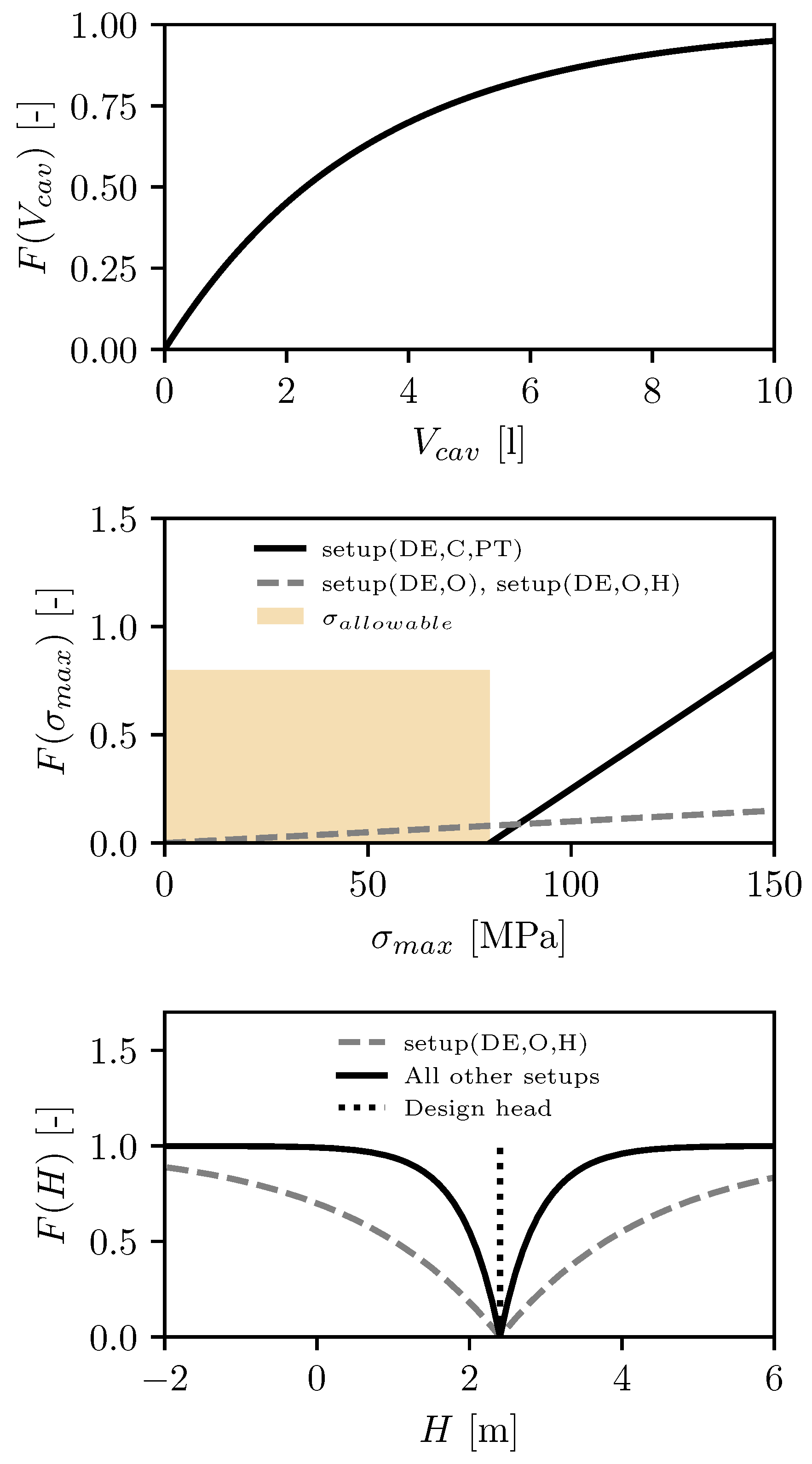
Figure 5.
Flow chart of the optimization process using the island model.
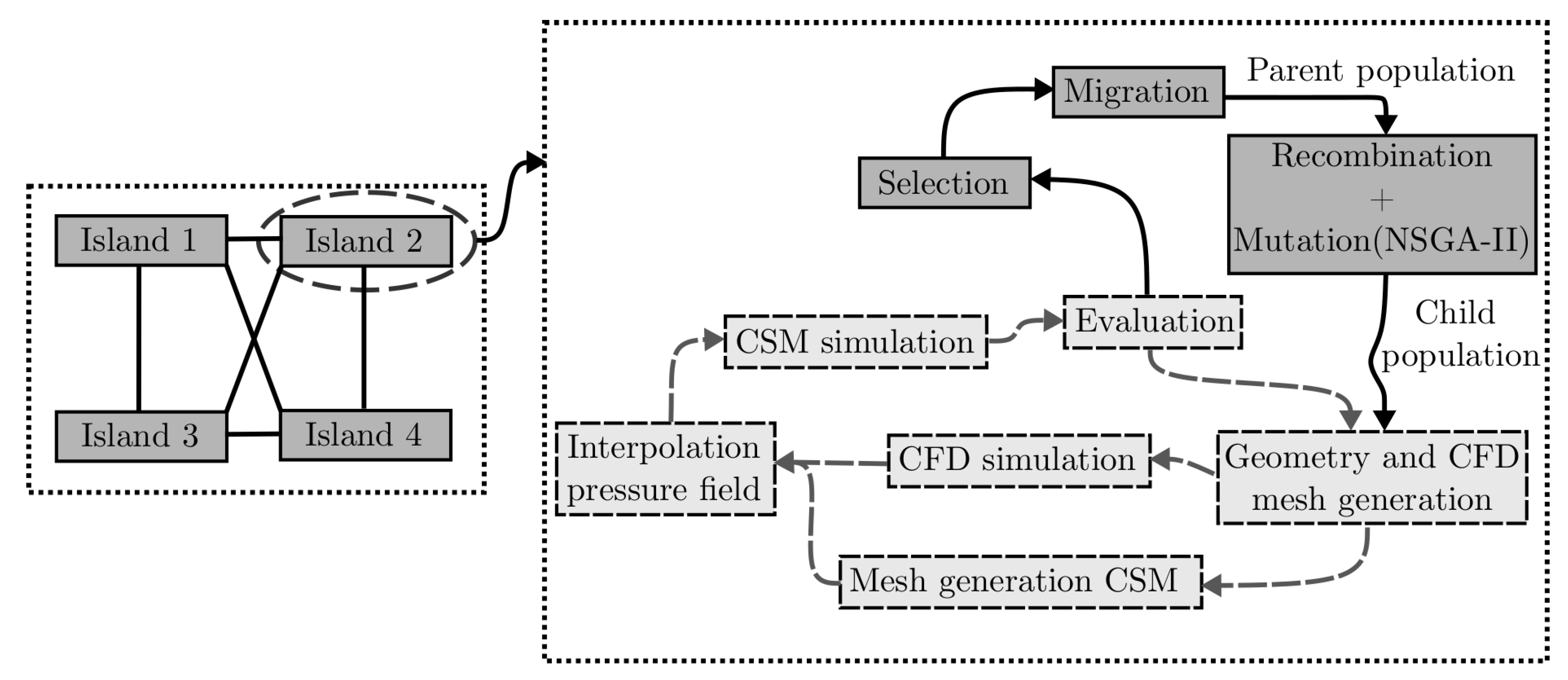
Figure 6.
Results of the optimization setups for the fitness calculated according to setup(DE,C,PT); Total mean fitness value with confidence interval and total mean fitness value expressed as equivalent efficiency
Figure 6.
Results of the optimization setups for the fitness calculated according to setup(DE,C,PT); Total mean fitness value with confidence interval and total mean fitness value expressed as equivalent efficiency
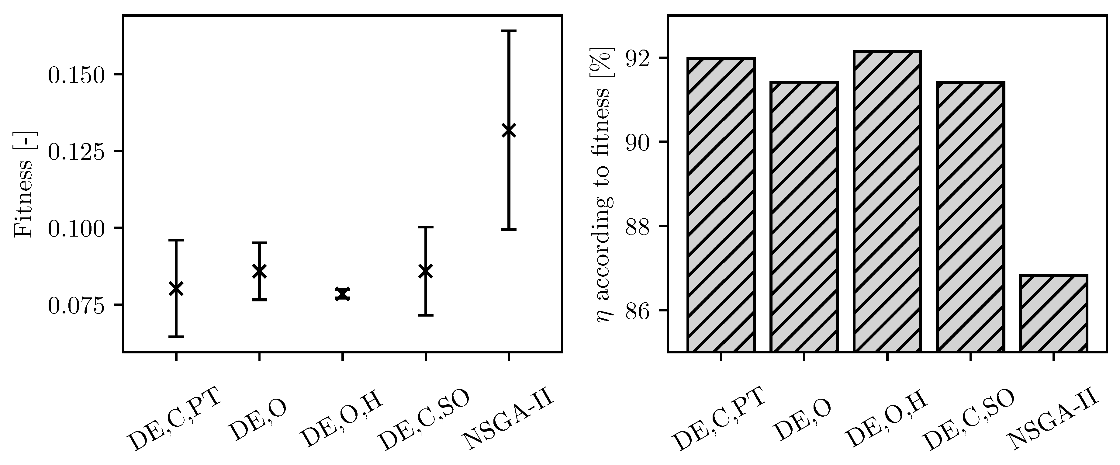
Figure 7.
Evolution of the maximum von Mises stress at full load, head at nominal operating point and averaged efficiency over the generations for setup(DE,C,PT), setup(DE,O) and setup(DE,O,H)
Figure 7.
Evolution of the maximum von Mises stress at full load, head at nominal operating point and averaged efficiency over the generations for setup(DE,C,PT), setup(DE,O) and setup(DE,O,H)
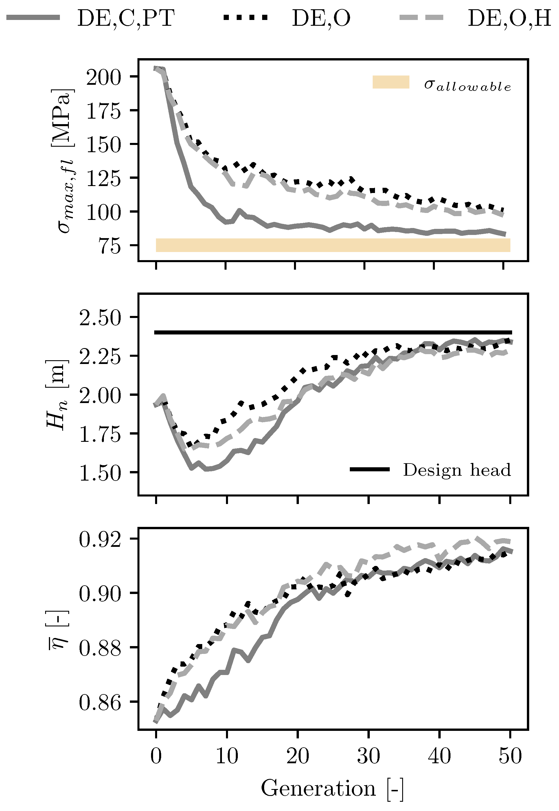
Figure 8.
Evolution of the CFD fitness without structural mechanical aspects, maximum von Mises stress at full load and head over generations for setup(DE,C,PT) and setup(DE,C,SO)
Figure 8.
Evolution of the CFD fitness without structural mechanical aspects, maximum von Mises stress at full load and head over generations for setup(DE,C,PT) and setup(DE,C,SO)
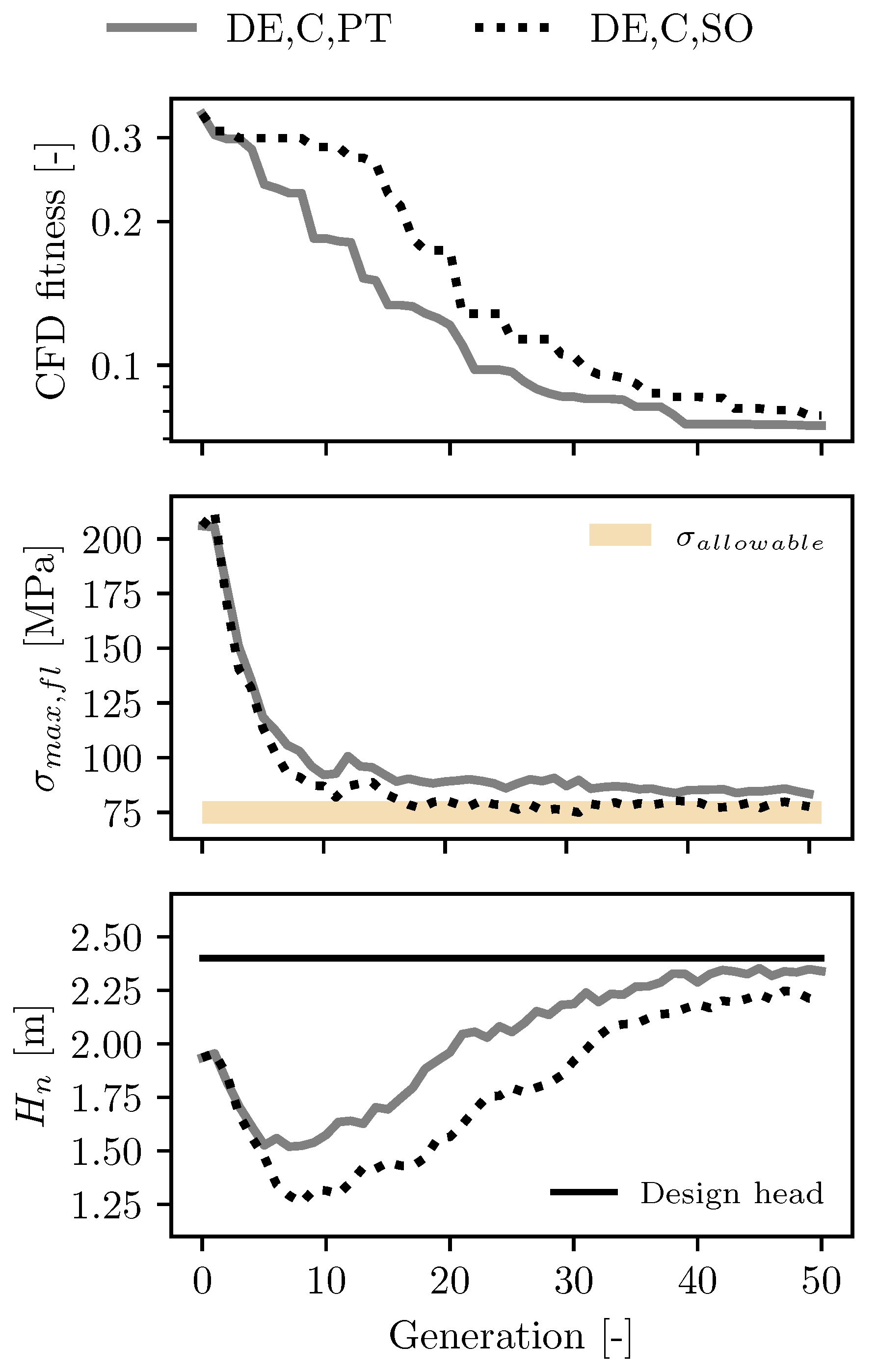
Figure 9.
Pareto fronts obtained for setup(NSGA-II); Averaged cavitation volume and maximum von Mises stress at full load over averaged efficiency
Figure 9.
Pareto fronts obtained for setup(NSGA-II); Averaged cavitation volume and maximum von Mises stress at full load over averaged efficiency
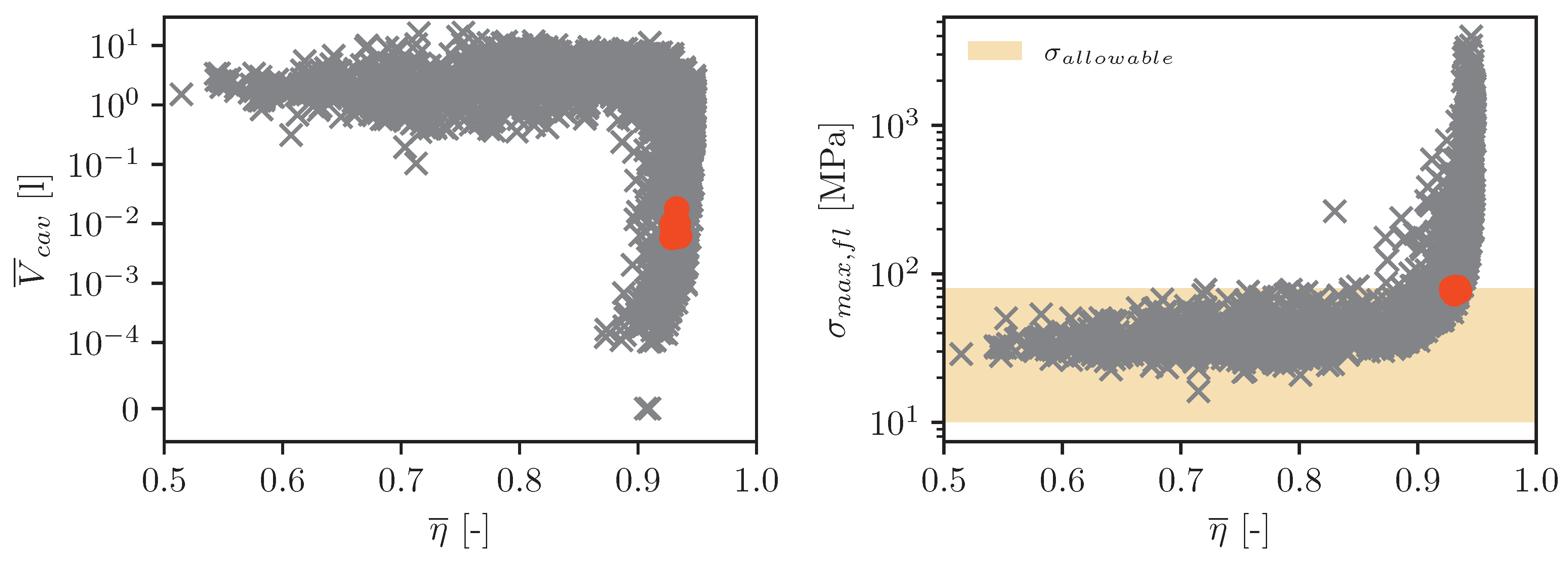

Table 1.
Optimization setups using a scalar objective function.
| Integration structural mechanics | |
|---|---|
| setup(DE,C,PT) | Constraint, penalty term |
| setup(DE,C,SO) | Constraint, selection operator |
| setup(DE,O) | Objective |
| setup(DE,O,H) | Objective, lower weighted head |
Disclaimer/Publisher’s Note: The statements, opinions and data contained in all publications are solely those of the individual author(s) and contributor(s) and not of MDPI and/or the editor(s). MDPI and/or the editor(s) disclaim responsibility for any injury to people or property resulting from any ideas, methods, instructions or products referred to in the content. |
© 2025 by the authors. Licensee MDPI, Basel, Switzerland. This article is an open access article distributed under the terms and conditions of the Creative Commons Attribution (CC BY) license (http://creativecommons.org/licenses/by/4.0/).
Copyright: This open access article is published under a Creative Commons CC BY 4.0 license, which permit the free download, distribution, and reuse, provided that the author and preprint are cited in any reuse.


