Submitted:
07 August 2025
Posted:
08 August 2025
You are already at the latest version
Abstract
In this work, the ground and low-lying excited states in a GaAs coupled quantum dot-ring embedded in an AlGaAs cylindrical matrix are computed under the assumption of a finite confinement potential and an axisymmetric model by means of the finite element method and the effective mass approximation. The electron energy levels are studied as functions of the intensity of externally applied electric and magnetic fields. Electromagnetically induced transparency in the ladder configuration and linear optical absorption coefficient are calculated thereupon. Our results suggest that magnetic fields are more suitable than electric fields for controlling the optical properties of this nanostructure.
Keywords:
coupled quantum dot-ring
; electronic states
; electric field effects
; magnetic field effects
; optical absorption coefficient
; electromagnetically induced transparency
1. Introduction
Quantum nanostructures such as quantum dots [1,2,3], lens-shaped structures [4,5,6], and tetrapods [7] exhibit unique electronic and optoelectronic properties, which make them suitable for applications in multiple fields, from bioimaging [8] to photovoltaics [9]. Among these, quantum rings (QR) [10,11,12] have attracted particular interest due to their unique electronic and optical characteristics, including Aharonov-Bohm oscillations and quantum interference effects [13,14], which open possibilities for their integration into optoelectronic devices and quantum information technologies [15,16,17].
During the characterization and fabrication process of such structures, it has been possible to experiment with various geometries [18,19,20,21], many of which are based on coupling structures. In recent years, coupled quantum dot-ring (CQDR) systems [22,23,24,25] have attracted significant attention due to their highly tunable electronic states, which can be modified by external factors such as electric and magnetic fields, hydrostatic pressure, and structural parameters [26]. This tunability makes CQDRs promising candidates for applications in optoelectronic devices, optical modulators [27], and quantum communication technologies [28]. These structures, formed by a QR coupled to a concentric quantum dot (QD), offer a versatile way to explore quantum interference phenomena and electromagnetically induced transparency (EIT).
CQDRs have also gained relevance due to their ability to host localized electronic states with versatile optical properties [24,26,29,30]. External perturbations on the structure, such as electric and magnetic fields, can substantially modify the electronic structure of these systems [31,32,33,34]. For example, the application of an electric field along the growth direction introduces Stark shifts and dipole moment variations [35,36,37]. This motivates continued studies that include these external perturbations.
Recent studies on the interaction between donors and structures have yielded interesting conclusions. Some have concluded that the interaction between the confined electron and the neutral donor center results in position-dependent modifications to transition energies and absorption properties[32,38,39]. Shallow donors add a layer of complexity to CQDRs due to their position within the structure [40,41], which plays a critical role in shaping electronic states and optical absorption spectra. Furthermore, recent studies on doubly ionized donors confined in CQDRs have provided information on the role of donor states and their interaction with external probes, such as hydrostatic pressure, electric fields, and temperature variations [26]. The present study explores the interaction between a shallow donor and a CQDR.
Such facts motivate the present study of the energy levels of a As CQDR, along with a detailed analysis of the consequences of external factors, such as magnetic and electric fields, while identifying the optoelectronic properties of the heterostructure. Furthermore, the study examines the phenomenon of EIT, in which quantum interference suppresses absorption while maintaining significant nonlinear optical properties [42,43].
This paper is organized as follows: in Section 2, we describe the theoretical model, outlining the fundamental principles that govern the electronic and optical properties of CQDRs, along with a description of the basic theory. Section 3 presents and discusses our numerical results, highlighting the impact of external perturbations and structural parameters on the electronic states and optical responses. Finally, our main conclusions are provided in Section 4.
2. Theoretical Framework
In this work, we analyze the energy states and their associated wavefunctions in a CQDR structure under the influence of external electric and/or magnetic fields applied in the z-direction. To complete our study, we investigate optoelectronic properties via EIT in a ladder or cascade configuration and linear optical absorption.
Figure 1 presents a schematic view of the CQDR under study, together with the main dimensions of the heterostructure. A 3D view of the nanostructure is shown in panel (a), obtained by revolution around the z-axis of Figure 1(b). A cross-section of the structure (the plane) is shown in panel (b), where the two composing materials are easily identified, i.e., the GaAs and the As. The latter displays a barrier-like behavior, while the former presents a well-like behavior. This configuration is suitable for building a 2D-axisymmetric model where azimuthal symmetry reduces the computational cost of numerically solving the three-dimensional Schrödinger equation. The geometry of the nanostructure is a variation of a theoretical function [32] that accurately reproduces an experimental profile of a GaAs CQDR, as obtained via the AFM technique by Somaschini [24]. To enhance the visibility of the ring’s influence, the height of the central region (dot) has been deliberately reduced by 65% compared to the original geometry. For the sake of clarity, the reference system and the directions of the external fields are also depicted. The CQDR is made of GaAs, whereas the cylindrical host matrix in which it is embedded is made of As with .
The mathematical function describing the height, , as depicted in Figure 1 (a), is formally expressed as[26]:
In this equation, represents the height of the central dot, denotes its characteristic width, signifies the height of the ring, corresponds to the radius of the ring, indicates the width of the ring and establishes the baseline height. For the specific nanostructure under investigation, the precise values assigned to these parameters are as follows: , , , , , and .
Using the effective mass approximation and taking the assumption of parabolic conduction bands, the Schrödinger equation of an electron interacting with external electric and magnetic fields is written in cylindrical coordinates as follows:
where i designates each of the quantized states, i.e., the value represents the ground state and corresponds to the excited states. The j-index identifies each one of the two materials that make up the CQDR, and e is the absolute value of the electron charge. The values of the effective mass and depend on the region where the Schrödinger equation is solved, as shown in Figure 1 (a). The effective mass is considered to be position-independent within each material. The effective mass and the confining potential are taken for the calculations in the following way:
and
In this work, both electric and magnetic fields are applied along the z-direction, i.e., and .
The gauge chosen for the description of the magnetic field effect entails the following conditions for the magnetic vector potential, : (i) and (ii). Under these two conditions, the Hamiltonian in Eq. 2 takes the form:
This Hamiltonian is separable, , which allows to replace in Eq. 5 (here ). Taking the derivatives with respect to , the Schrödinger equation for the radial function can be written as:
where are the eigenvalues associated with the 2D-wavefunctions . The solution of Eq. 6 was investigated using the finite element method (FEM) as implemented in the COMSOL-Multiphysics software [44]. The boundary conditions were imposed in the following way: (i) BenDaniel-Duke boundary condition for wave function continuity on the core-shell interface, , (ii) BenDaniel-Duke boundary condition for the wave function first derivative continuity: with and (iii) Dirichlet boundary conditions on the outer surface of the embedding As matrix: .
The cascade configuration chosen for the EIT analysis comprises the first three energy levels and is modeled in Figure 2.
Within the density matrix approach, an expression for the imaginary part of the linear susceptibility can be derived in terms of the probe field and Rabi frequencies as follows [31]:
where is the detuning between the probe field frequency and that of the transition,
is the electric dipole matrix element for a transition between states and induced by a light field with polarization vector . While the general notation uses indices , the specific transition from the ground state to the first excited state () is represented by the element , as shown in the formula, is the Rabi frequency associated with the aforementioned transition, stands for the population difference between the two involved levels, and are the decay rates for the transition. The Rabi frequency is taken to be fixed for the material throughout this study. The imaginary part of the linear susceptibility is related to the linear optical absorption, allowing for the EIT calculation as in [31]:
where is the speed of light in the medium, . Finally, the linear optical absorption coefficient (LOAC) for the transition can be deduced from Eq. 8, subtracting all contributions coming from the third level, i. e., , .
To close this section, we provide in Figure 3 the comparison of the first ten electron eigenenergies obtained by solving the three-dimensional Schrödinger equation, by implementing the adiabatic approximation, and through the 2D-axisymmetric model described along this section. The use of the adiabatic approximation is justified by the system’s morphological features, where confined carriers experience significantly greater quantum confinement in the z-direction than in the plane [32]. This geometric asymmetry supports the decoupling of the electron’s motion into two separate kinetic contributions (z-axis and -plane). The procedure begins by "freezing" the -plane motion to solve a one-dimensional Schrödinger equation for the z-axis. The resulting eigenvalues are then introduced into the -plane Schrödinger equation, reducing the original three-dimensional Hamiltonian to a simplified and numerically solvable two-dimensional problem.
As Figure 3 shows, the results from all three methods are in very good agreement, the 3D model being the most precise. Therefore, we can confidently conclude that the implementation of the simpler axisymmetric model is justified for our analysis. At this point, it is worth mentioning that the fact of having seven eigenstates with similar energies does not mean a seven-fold degeneracy, given that the eigenenergies associated with the dot are mixed with those associated with the ring. The latter will be thoroughly discussed later on.
3. Results and discussion
The Schrödinger equation, given in Eq. 6, was solved using the FEM via the COMSOL-Multiphysics software [44] within the effective mass approximation. We computed the lowest confined electron energy states in a GaAs CQDR embedded in an As cylindrical matrix with applying external electric and/or magnetic fields perpendicular to the structure. We calculated the EIT and the LOAC in the presence and absence of the fields mentioned above. The parameters for electrons adopted in the numerical calculations are , (here, is the free electron mass) [45] and the barrier height of meV [46]. Calculations were performed for negative and positive values of the electric field F. The CQDR profile under study is an adaptation of AFM measurements [24]. In the first stage, the study will focus on analyzing the effects of electric and/or magnetic fields on electron energy levels when the fields are applied perpendicular to the structure.
Figure 4 shows the variation in the electron energies of the first states obtained by applying an electric field directed along the z-axis. Negative field values indicate that the field points in the negative z-direction. The implementation of a 2D-axisymmetric model allows the distinction of states according to the quantum number l. In this work, the first states with are analyzed. Panel (a) of Figure 4 is devoted to the case in which no magnetic field is applied, and, therefore, the states with positive (solid lines) and negative (dashed lines) l are superimposed, as is straightforward from Eq. 6. The energy of the states increases as the electric field shifts from negative to positive values, given that the electron wave function is pushed towards the lower region of the CQDR, becoming more confined as the field intensity increases. The following states, after the first and states, which correspond to the dot, are concentrated in less than 5 meV. Here, the ring states appear and are intermixed with the dot states. To complete this analysis, panel (b) shows the energy variation with the electric field in the presence of a magnetic field, also applied along the z-direction. This magnetic field is responsible for the degeneracy breaking of the energies associated with and . Comparing panels (a) and (b) of Figure 4, states with () are found to display higher (lower) energies than in the absence of the magnetic field. At the same time, all of them show increasing energies as the electric field intensity ranges from more negative to more positive values. In both the absence and the presence of an external magnetic field, a linear increasing trend in the energy levels is observed as the electric field ranges from to kV/cm, such that the levels are practically parallel. A linear fit of these allows the calculation of an average slope, which, in the case of a zero magnetic field, is meV cm/kV, while in the case of a T magnetic field it is of meV cm/kV. The relative standard deviation in the first case is and in the second case is . The value of this slope can be related to the Stark shift [47,48].
For the sake of completeness, the variation in electron energy is now analyzed in the presence of an externally applied magnetic field, both in the absence and in the presence of an electric field, with both fields parallel to the z-axis. The results are shown in Figure 5, which distinguishes the states based on the quantum number l, as previously discussed. Both levels whose energy decreases with the magnetic field (typically of QDs) and levels whose energy increases (typically of QRs) are observed. Panels (a) and (c) show the first electron energies as a function of the magnetic field without an electric field and with an electric field of kV/cm applied to the nanostructure, respectively. From the comparison between them, it is concluded that the electric field does not alter the main features of the electronic structure, but increases the energies associated with all states. As discussed in Figure 4, the accumulation of states observed corresponds to the emergence of the ring states. Panels (b) and (d) correspond to a zoom of the shadow region in panels (a) and (c), respectively. The Aharanov-Bohm oscillations, typical of this kind of structure [49], are observed.
The energy spectrum observed in Figure 5 can be better understood by decomposing the CDQR into a colloidal quantum dot (CQD) and a colloidal quantum ring (CQR) with the same wetting layer and dimensions as those shown in Figure 1. The results of this decomposition are shown in Figure 6, where panel (a) corresponds to the CQD and panel (b) corresponds to the CQR. The magnetic field sweep is selected according to panels (a) and (c) of Figure 5. For simplicity, only the case with no external electric field applied to the nanostructure is analyzed. The superposition of panels (a) and (b) of Figure 6 is shown in panel (c), from which it is clear that the results obtained for the CQDR in Figure 5 (a) and (c) are consistent with the aforementioned decomposition of the nanostructure, where the coupling between its components causes them to interact and exhibit slight differences.
The second part of this work is devoted to calculating the EIT in the ladder configuration and LOAC for various values of the electric and magnetic fields.
To begin with, Figure 7 illustrates the EIT calculation as a function of the probe field energy, , and the LOAC as a function of the incident photon energy, , for three different values of the electric field with and without a magnetic field applied to the nanostructure. Looking at panel (a) of Figure 7, it is straightforward that the two peaks associated with the EIT present a slightly appreciable blueshift as the absolute value of the electric field increases. Additionally, it is worth noting that the magnitude of the peaks also increases with the absolute value of the electric field. Finally, a particularity arises for the positive value of the electric field, where no EIT is observed. The latter is due to the term of the electric dipole moment matrix corresponding to the transitions involved in the ladder configuration, i.e., between the ground and the first two excited states. This kind of EIT requires an allowed transition and a nearly suppressed transition. The panel (a) of Figure 6 illustrates how these matrix terms change their behavior at approximately kV/cm, making zero the EIT for positive F-values. The blueshift is justified by the energy levels features shown in Figure 4 (a). When a magnetic field T is applied together with the electric field, the EIT in the ladder configuration is observed for positive and negative values of the electric field. This is illustrated on panel (b) of Figure 7 and is justified by the dipole moment matrix terms displayed in Figure 8(b). A slight blueshift occurs as the electric field ranges from positive to negative values. On the other hand, shadowed regions on panels (a) and (b) of Figure 7 show the LOAC as a function of the incident photon energy, which is centered at the minimum located between the two EIT peaks. Again, the term of the zero electric dipole matrix for the transition at positive electric field values is responsible for the zero LOAC in (a).
The behavior of the dipole matrix terms shown in Figure 8, which directly impacts the EIT spectra in Figure 7, is governed by the energy shifts of the electronic states under external fields. To illustrate this dependence, Figure 9 plots the energies of the first three states with angular momentum , denoted as (where is the principal quantum number and ), as a function of the applied electric field. Panel (a) shows the case without a magnetic field (B = 0 T), while panel (b) corresponds to a magnetic field (B = 10 T). The gray shaded areas indicate the specific electric field values used for the calculations in Figure 7.
To better visualize the non-linear component of the Stark effect, which is crucial for determining the dipole moments, a dominant linear trend has been subtracted from the energy values. This data processing step allows the quadratic shifts and level anti-crossings which are otherwise obscured to be clearly observed, providing a direct insight into the physics governing the dipole matrix elements.
Figure 10 illustrates the dependence of the EIT and LOAC on the magnetic field, both in the absence and presence of an external electric field. Panel (a) shows the results for a zero electric field, it is clear that the EIT peaks shift toward higher energies as the magnetic field strength increases and that the LOAC peaks undergo the same energy shift. Panel (b) is homologous to (a), but subjecting the system to an external electric field of kV/cm. Comparing the EIT and LOAC peaks in both panels, it is straightforward that the effect of the electric field is practically negligible compared to the magnetic field, with only a slight variation in the magnitude and position of the peaks being observed. The magnitude of the EIT peaks decreases slightly between (a) and (b), and the shift of the peaks to lower energies in the presence of the electric field is practically imperceptible. The electric field causes once more the emergence of the LOAC peaks at lower energies and their magnitude to be slightly lower compared to the case without the electric field. All this is justified by the electronic structure shown in Figure 5.
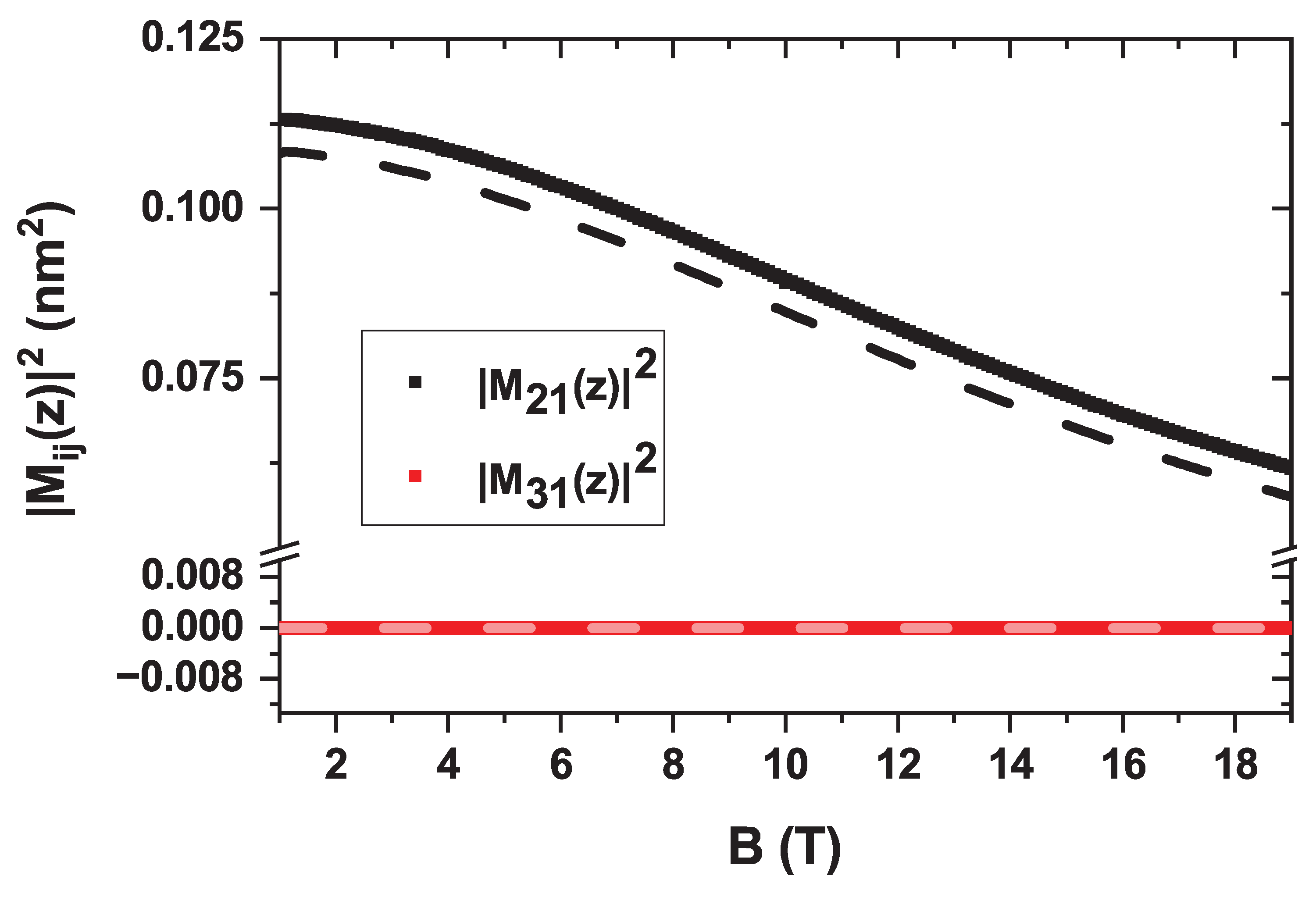
In contrast to Figure 7, the non-zero EIT shown in Figure 10 is explained by the behavior of the electric dipole matrix elements, which are depicted in Figure 11. This figure displays the squared dipole moments for the transition () and the transition () as a function of the magnetic field. The results are shown for both a zero electric field (solid lines) and an external electric field of kV/cm (dashed lines).
A direct comparison between the solid and dashed curves reveals that the influence of the electric field on the dipole moments is minimal, confirming that the system’s optical response is predominantly governed by the magnetic field. The most significant trend observed is the systematic decrease of the primary dipole matrix element, , as the magnetic field strength increases. This behavior is a direct consequence of magnetic confinement. The applied Lorentz force radially compresses the electron wavefunctions, leading to a reduced spatial overlap for the dipole transition. Consequently, the magnitude of is diminished, which directly suppresses the transition probability and, therefore, the overall absorption intensity [50]. It is also noteworthy that the element is nearly zero across the entire range, indicating that the transition is dipole-forbidden for this light polarization, consistent with the selection rules.
4. Conclusions
In this study, we have analyzed the electronic structure and optical properties of a As CQDR system under the influence of external electric and magnetic fields. Using a finite element method within the effective mass approximation, we have demonstrated that both fields significantly influence the confined electron energy levels, with the magnetic field producing notable Aharonov-Bohm oscillations and a more substantial impact on the energy spectrum than the electric field. These external fields not only shift the electronic states but also modulate the LOAC and EIT behavior, thereby providing mechanisms for dynamic control of the nanostructure’s optoelectronic response.
The EIT phenomenon in a ladder configuration was thoroughly investigated, revealing that its occurrence and intensity are highly sensitive to the direction and magnitude of the applied electric field. In particular, a suppression of EIT was observed for positive electric field values in the absence of a magnetic field, an effect traced to vanishing dipole transition matrix elements. Conversely, applying a magnetic field restored the EIT for all electric field values, leading to an overall enhancement in the tunability of optical transparency and absorption. These findings highlight the superior role of magnetic fields in precisely modulating light-matter interactions in CQDRs.
Overall, our results demonstrate that CQDR systems are promising platforms for developing tunable optoelectronic devices, with magnetic fields offering a more robust control parameter than electric fields for manipulating EIT and LOAC. These findings contribute to the understanding of quantum interference effects in complex nanostructures, opening pathways for their application in photonic devices and quantum information processing technologies.
Author Contributions
R. V. H. Hahn: Conceptualization, Methodology, Software, Validation, Formal Analysis, Investigation, Data curation, Writing - Review and Editing, Visualization. A. S. Giraldo-Neira: Conceptualization, Methodology, Software, Validation, Formal Analysis, Investigation, Data curation, Writing - Review and Editing, Visualization. J. A. Vinasco: Conceptualization, Methodology, Software, Validation, Formal Analysis, Investigation, Data curation, Writing - Review and Editing, Visualization. J. A. Gil-Corrales: Conceptualization, Methodology, Software, Validation, Formal Analysis, Investigation, Data curation, Writing - Review and Editing, Visualization. A. L. Morales: Conceptualization, Formal Analysis, Writing - Review and Editing, Visualization. C. A. Duque: Conceptualization, Formal Analysis, Writing - Review and Editing, Visualization.
Data Availability Statement
All the files with tables, figures, and codes are available. The corresponding author will provide all the files in case they are requested.
Acknowledgments
The authors are grateful to Colombian agencies CODI-Universidad de Antioquia (Estrategia de Sostenibilidad de la Universidad de Antioquia and projects “Complejos excitónicos y propiedades de transporte en sistemas nanométricos de semiconductores con simetría axial basados en GaAs e InAs”, and "Nanoestructuras semiconductoras con simetría axial basadas en InAs y GaAs para aplicaciones en electrónica ultra e híper rápida") and Facultad de Ciencias Exactas y Naturales-Universidad de Antioquia (C.A.D. exclusive dedication project 2025-2026). R. V. H. H. gratefully acknowledges financial support from the Spanish Junta de Andalucía through a Doctoral Training Grant PREDOC-01408.
Conflicts of Interest
The authors do not have any financial and non-financial competing interests statement.
References
- Lorke, A.; Kotthaus, J.P.; Ploog, K. Coupling of quantum dots on GaAs. Phys. Rev. Lett. 1990, 64, 2559–2562. [Google Scholar] [CrossRef] [PubMed]
- Abdelsalam, H.; Elhaes, H.; Ibrahim, M.A. Tuning electronic properties in graphene quantum dots by chemical functionalization: Density functional theory calculations. Chem. Phys. Lett. 2018, 695, 138–148. [Google Scholar] [CrossRef]
- de Queiroz, A.A.A.; Martins, M.; Soares, D.A.W.; França, J. Modeling of ZnS quantum dots synthesis by DFT techniques. J. Mol. Struct. 2008, 873, 121–129. [Google Scholar] [CrossRef]
- Lew Yan Voon, L.C.; Willatzen, M. Confined states in lens-shaped quantum dots. Physica B 2002, 14, 13667. [Google Scholar] [CrossRef]
- Khordad, R. Electronic and Optical Properties of a Lens Shaped Quantum Dot under Magnetic Field: Second and Third-Harmonic Generation. Commun. Theor. Phys. 2014, 62, 283. [Google Scholar] [CrossRef]
- Vahdani, M.R.K.; Rezaei, G. Linear and nonlinear optical properties of a hydrogenic donor in lens-shaped quantum dots. Phys. Lett. A 2009, 373, 3079–3084. [Google Scholar] [CrossRef]
- Hahn, R.V.H.; Mora-Rey, F.; Restrepo, R.L.; Morales, A.L.; Montoya-Sánchez, J.; Eramo, G.; Barseghyan, M.G.; Ed-Dahmouny, A.; Vinasco, J.A.; Duque, D.A.; et al. Electronic and optical properties of tetrapod quantum dots under applied electric and magnetic fields. Eur. Phys. J. Plus 2024, 139, 344. [Google Scholar] [CrossRef]
- Pandey, S.; Bodas, D. High-quality quantum dots for multiplexed bioimaging: A critical review. Adv. Colloid Interface Sci. 2020, 278, 102137. [Google Scholar] [CrossRef]
- Semonin, O.E.; Luther, J.M.; Beard, M.C. Quantum dots for next-generation photovoltaics. Mater. Today 2012, 15, 508–515. [Google Scholar] [CrossRef]
- Hossain, M.A.; Khoo, K.T.; Cui, X.; Poduval, G.K.; Zhang, T.; Li, X.; Li, W.M.; Hoex, B. Atomic layer deposition enabling higher efficiency solar cells: A review. Nano Mater. Sci. 2020, 2, 204–226. [Google Scholar] [CrossRef]
- Silva, G.F.; Ulloa, S.E.; Faria, P., Jr. E. Topological States in Rashba-Dresselhaus Quantum Rings with Broken Symmetry. Physica E 2025, 168, 116345. [Google Scholar] [CrossRef]
- Ivanov, D.; Kovalev, A.; Peeters, F.M. Valley-Polarized States in Graphene Quantum Rings on a Hexagonal Boron Nitride Substrate. Phys. Rev. Lett. 2025, 134, 156804. [Google Scholar] [CrossRef]
- Michal, V.P.; Fujita, T.; Baart, T.A.; Danon, J.; Reichl, C.; Wegscheider, W.; Vandersypen, L.M.K.; Nazarov, Y.V. Nonlinear and dot-dependent Zeeman splitting in GaAs/AlGaAs quantum dot arrays. Phys. Rev. B 2018, 97, 035301. [Google Scholar] [CrossRef]
- Li, J.; Singh, A.; D’Souza, M. Tunable Aharonov-Bohm Oscillations in Vertically Stacked Ge/Si Quantum Rings. Nano Lett. 2025, 25, 1245–1251. [Google Scholar] [CrossRef]
- Xia, H.; Hu, H.; Wang, Y.; Yu, M.; Yuan, M.; Yang, J.; Gao, L.; Zhang, J.; Tang, J.; Lan, X. Ligand-customized colloidal quantum dots for high-performance optoelectronic devices. J. Mater. Chem. C 2024, 12, 10919–10928. [Google Scholar] [CrossRef]
- Zhang, L.; Bauer, G.E.W.; Tserkovnyak, Y. Spin Pumping and Inverse Spin Hall Effect in Ferromagnet-Quantum Ring Hybrid Structures. Nat. Commun. 2025, 16, 257. [Google Scholar] [CrossRef]
- Wang, F.; Rodriguez, C.; Gupta, A. Terahertz Photodetection in Concentric GaN/AlN Quantum Ring Arrays. Appl. Phys. Lett. 2025, 126, 031105. [Google Scholar] [CrossRef]
- Dahiya, V.; Zamiri, M.; So, M.G.; Hollingshead, D.A.; Kim, J.S.; Krishna, S. Fabrication of InAs quantum ring nanostructures on GaSb by droplet epitaxy. J. Cryst. Growth 2018, 492, 71–76. [Google Scholar] [CrossRef]
- Surrente, A.; Carron, R.; Gallo, P.; Rudra, A.; Dwir, B.; Kapon, E. Self-formation of hexagonal nanotemplates for growth of pyramidal quantum dots by metalorganic vapor phase epitaxy on patterned substrates. Nano Res. 2016, 9, 3279–3290. [Google Scholar] [CrossRef]
- Tanaka, K.; Ito, H.; Nakamura, Y. Droplet Epitaxy of InSb Quantum Dot-in-a-Ring Structures for Mid-Infrared Applications. J. Cryst. Growth 2025, 650, 127890. [Google Scholar] [CrossRef]
- Patel, R.; Jackson, H.E.; Smith, L.M. Raman Spectroscopy of Individual CdSe/CdS Dot-in-Ring Nanocrystals. J. Phys. Chem. C 2025, 129, 8041–8048. [Google Scholar] [CrossRef]
- Boonpeng, P.; Kiravittaya, S.; Thainoi, S.; Panyakeow, S.; Ratanathammaphan, S. InGaAs quantum-dot-in-ring structure by droplet epitaxy. J. Cryst. Growth 2013, 378, 435–438. [Google Scholar] [CrossRef]
- Elborg, M.; Noda, T.; Mano, T.; Kuroda, T.; Yao, Y.; Sakuma, Y.; Sakoda, K. Self-assembly of vertically aligned quantum ring-dot structure by Multiple Droplet Epitaxy. J. Cryst. Growth 2017, 477, 239–242. [Google Scholar] [CrossRef]
- Somaschini, C.; Bietti, S.; Koguchi, N.; Sanguinetti, S. Coupled quantum dot-ring structures by droplet epitaxy. Nanotechnology 2011, 22, 185602. [Google Scholar] [CrossRef] [PubMed]
- Strom, N.W.; Wang, Z.M.; Lee, J.H.; Abuwaar, Z.Y.; Mazur, Y.I.; Salamo, G.J. Self-assembled InAs quantum dot formation on GaAs ring-like nanostructure templates. Nanoscale Res. Lett. 2007, 2, 112–117. [Google Scholar] [CrossRef]
- Hernández, N.; López-Doria, R.A.; Fulla, M.R. Optical and electronic properties of a singly ionized double donor confined in coupled quantum dot-rings. Physica E 2023, 151, 115736. [Google Scholar] [CrossRef]
- Farzin, M.A.; Abdoos, H. A critical review on quantum dots: From synthesis toward applications in electrochemical biosensors for determination of disease-related biomolecules. Talanta 2021, 224, 121828. [Google Scholar] [CrossRef]
- Vajner, D.A.; Rickert, L.; Gao, T.; Kaymazlar, K.; Heindel, T. Quantum Communication Using Semiconductor Quantum Dots. Adv. Quantum Technol. 2022, 5, 2100116. [Google Scholar] [CrossRef]
- Ahmad, Y.; Schulz, S.; O’Reilly, E.P. The role of interface asymmetry on the optical properties of coupled quantum rings. Physica B 2025, 37, 225301. [Google Scholar] [CrossRef]
- Chen, W.; Kim, M.j.; Santos, D.; Petrović, M. Spin-Orbit Interaction in Asymmetric InAs/GaAs Double Quantum Rings. Phys. Rev. B 2025, 111, 075301. [Google Scholar] [CrossRef]
- Scully, M.O.; Zubairy, M.S. Quantum Optics; Cambridge University Press, 1997.
- Hernández, N.; López-Doria, R.A.; Suaza, Y.A.; Fulla, M.R. Neutral donors confined in semiconductor coupled quantum dot-rings: Position-dependent properties and optical transparency phenomenon. Physica E 2025, 165, 116122. [Google Scholar] [CrossRef]
- Holleitner, A.W.; Decker, C.R.; Blick, R.H.; Eberl, K. Coherent Coupling of Two Quantum Dots Embedded in an Aharonov-Bohm Ring. Phys. Rev. Lett. 2001, 87, 256802. [Google Scholar] [CrossRef] [PubMed]
- Gonzalez, S.; Schmidt, O.G.; Rastelli, A. Controlling Exciton Coherence in Coupled Dot-Ring Systems via Strain Engineering. ACS Photonics 2025, 12, 512–519. [Google Scholar] [CrossRef]
- Mora-Ramos, M.E.; Vinasco, J.A.; Laroze, D.; Radu, A.; Restrepo, R.L.; Heyn, C.; Tulupenko, V.; Hieu, N.N.; Phuc, H.V.; Ojeda, J.H.; et al. Electronic structure of vertically coupled quantum dot-ring heterostructures under applied electromagnetic probes. A finite-element approach. Sci. Rep. 2021, 11, 4293. [Google Scholar] [CrossRef]
- Miller, D.A.B.; Chemla, D.S.; Damen, T.C.; Gossard, A.C.; Wiegmann, W.; Wood, T.H.; Burrus, C.A. Electric field dependence of optical absorption near the band gap of quantum-well structures. Phys. Rev. B 1985, 32, 1043–1060. [Google Scholar] [CrossRef]
- Huang, H.; Csontosová, D.; Manna, S.; Huo, Y.; Trotta, R.; Rastelli, A.; Klenovský, P. Electric field induced tuning of electronic correlation in weakly confining quantum dots. Phys. Rev. B 2021, 104, 165401. [Google Scholar] [CrossRef]
- Riva, C.; Escorcia, R.; Peeters, F.M. Neutral and charged donor in a 3D quantum dot. Physica E 2004, 22, 550–553. [Google Scholar] [CrossRef]
- Boda, A.; Chatterjee, A. Transition energies and magnetic properties of a neutral donor complex in a Gaussian GaAs quantum dot. Superlattices Microstruct. 2016, 97, 268–276. [Google Scholar] [CrossRef]
- Movilla, J.L.; Ballester, A.; Planelles, J. Coupled donors in quantum dots: Quantum size and dielectric mismatch effects. Phys. Rev. B 2009, 79, 195319. [Google Scholar] [CrossRef]
- Zhu, K.D.; Gu, S.W. Electric-field effects on shallow donor impurities in a harmonic quantum dot. Phys. Lett. A 1993, 181, 465–470. [Google Scholar] [CrossRef]
- Jiang, Y.W.; Zhu, K.D.; Wu, Z.J.; Yuan, X.Z.; Yao, M. Electromagnetically induced transparency in quantum dot systems. J. Phys. B: At., Mol. Opt. Phys. 2006, 39, 2621. [Google Scholar] [CrossRef]
- Barettin, D.; Houmark, J.; Lassen, B.; Willatzen, M.; Nielsen, T.R.; Mørk, J.; Jauho, A.P. Optical properties and optimization of electromagnetically induced transparency in strained InAs/GaAs quantum dot structures. Phys. Rev. B 2009, 80, 235304. [Google Scholar] [CrossRef]
- COMSOL AB. COMSOL Multiphysics v. 6.2. Stockholm, Sweden, 2023.
- Nakwaski, W. Effective masses of electrons and heavy holes in GaAs, InAs, AlAs and their ternary compounds. Physica B 1995, 210, 1–25. [Google Scholar] [CrossRef]
- Yamagiwa, M.; Sumita, N.; Minami, F.; Koguchi, N. Confined electronic structure in GaAs quantum dots. J. Lumin. 2004, 108, 379–383. [Google Scholar] [CrossRef]
- Heyn, C.; Ranasinghe, L.; Zocher, M.; Hansen, W. Shape-Dependent Stark Shift and Emission-Line Broadening of Quantum Dots and Rings. J. Phys. Chem. C 2020, 124, 19809–19816. [Google Scholar] [CrossRef]
- Khordad, R. Stark shift in a Frost-Musulin quantum dot: Analytical solution. Physica B 2024, 690, 416297. [Google Scholar] [CrossRef]
- Mora-Ramos, M.E.; Vinasco, J.A.; Radu, A.; Restrepo, R.L.; Morales, A.L.; Sahin, M.; Mommadi, O.; Sierra-Ortega, J.; Escorcia-Salas, G.E.; Heyn, C.; et al. Double Quantum Ring under an Intense Nonresonant Laser Field: Zeeman and Spin-Orbit Interaction Effects. Physica B 2023, 8, 79. [Google Scholar] [CrossRef]
- Reimann, S.M.; Manninen, M. Electronic structure of quantum dots. Rev. Mod. Phys. 2002, 74, 1283–1342. [Google Scholar] [CrossRef]
Figure 1.
Schematic representation of the As three-dimensional CQDR geometry (a), together with a -plane slice of the CQDR and the cylindrical boundary for visualization of the main dimensions of the heterostructure (b). The reference system and the directions of the externally applied electric and magnetic field are also depicted.
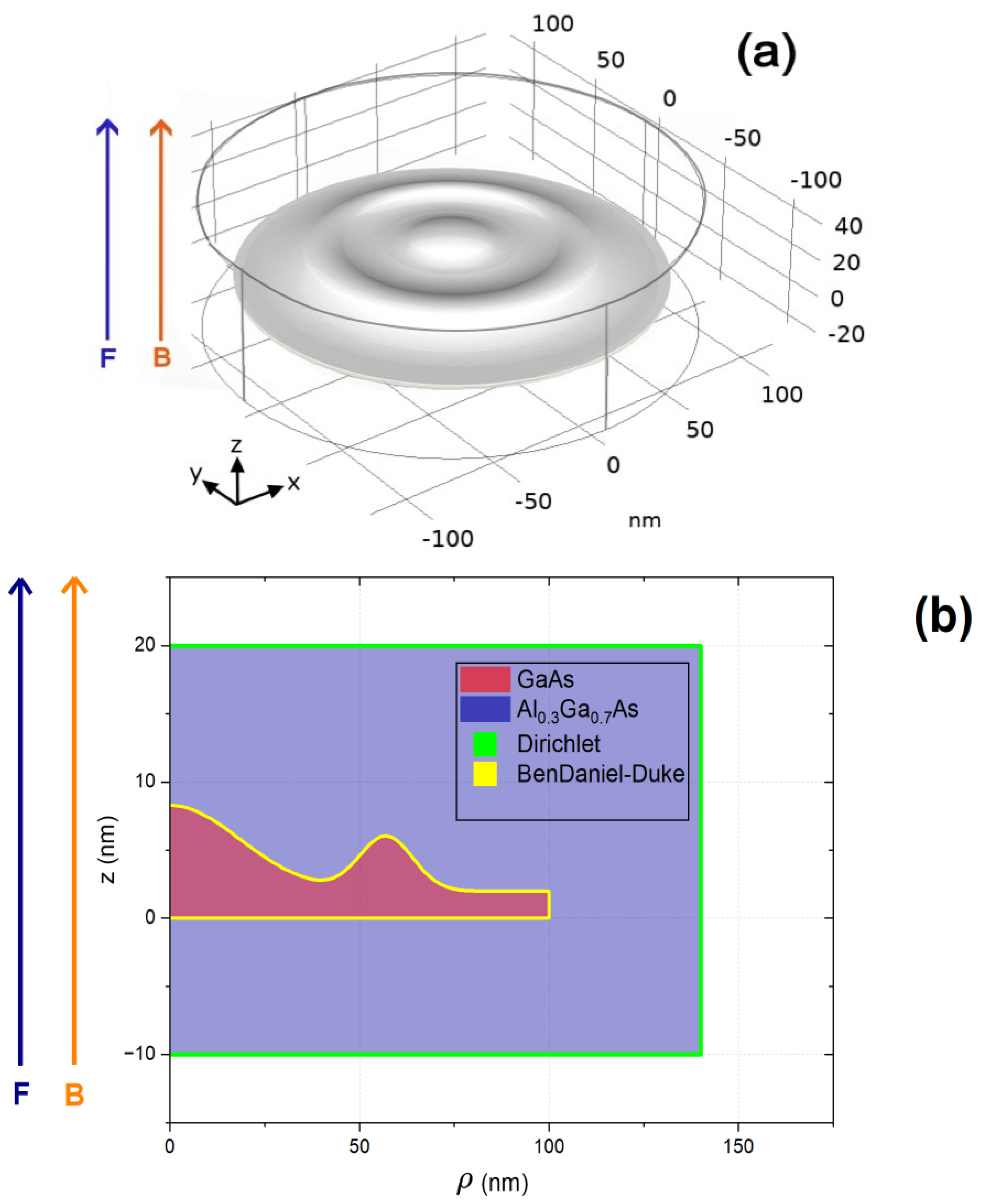
Figure 2.
Schematic diagram of the three-level system in a ladder or cascade configuration interacting with control and probe electromagnetic fields of frequencies and , respectively. For clarity, the detuning is also depicted.
Figure 2.
Schematic diagram of the three-level system in a ladder or cascade configuration interacting with control and probe electromagnetic fields of frequencies and , respectively. For clarity, the detuning is also depicted.
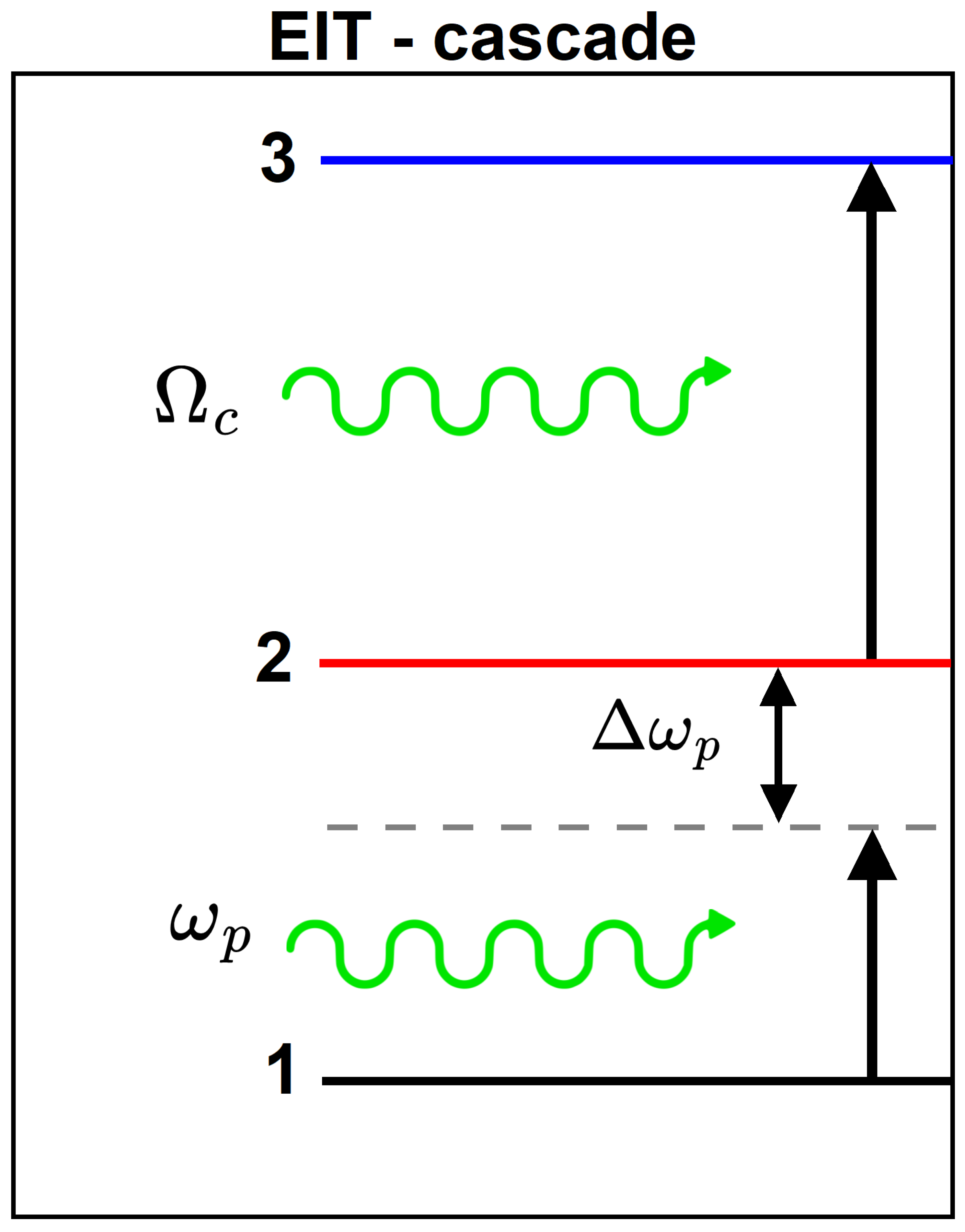
Figure 3.
First ten electron eigenenergies in the GaAs/AlGaAs CQDR structure obtained by the 2D-axisymmetric model (red), the adiabatic approximation (black), and the three-dimensional model (green).
Figure 3.
First ten electron eigenenergies in the GaAs/AlGaAs CQDR structure obtained by the 2D-axisymmetric model (red), the adiabatic approximation (black), and the three-dimensional model (green).
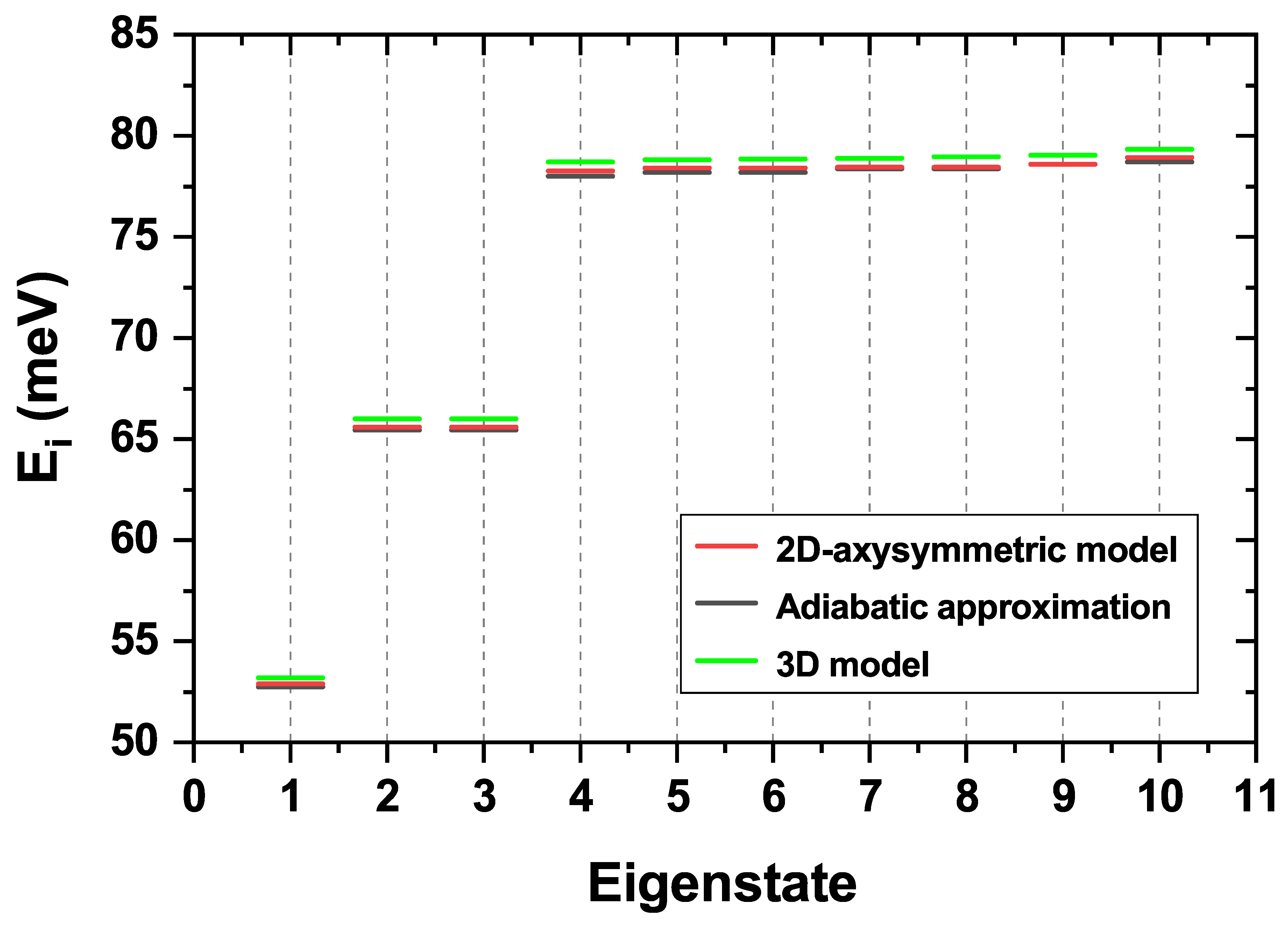
Figure 4.
Energy variation of the first low-lying electron states in the absence of magnetic field (a) and with an externally applied magnetic field of T along the z-axis (b), as a function of the external electric field, applied along the z-direction. The negative values of the electric field are related to the negative z-axis.
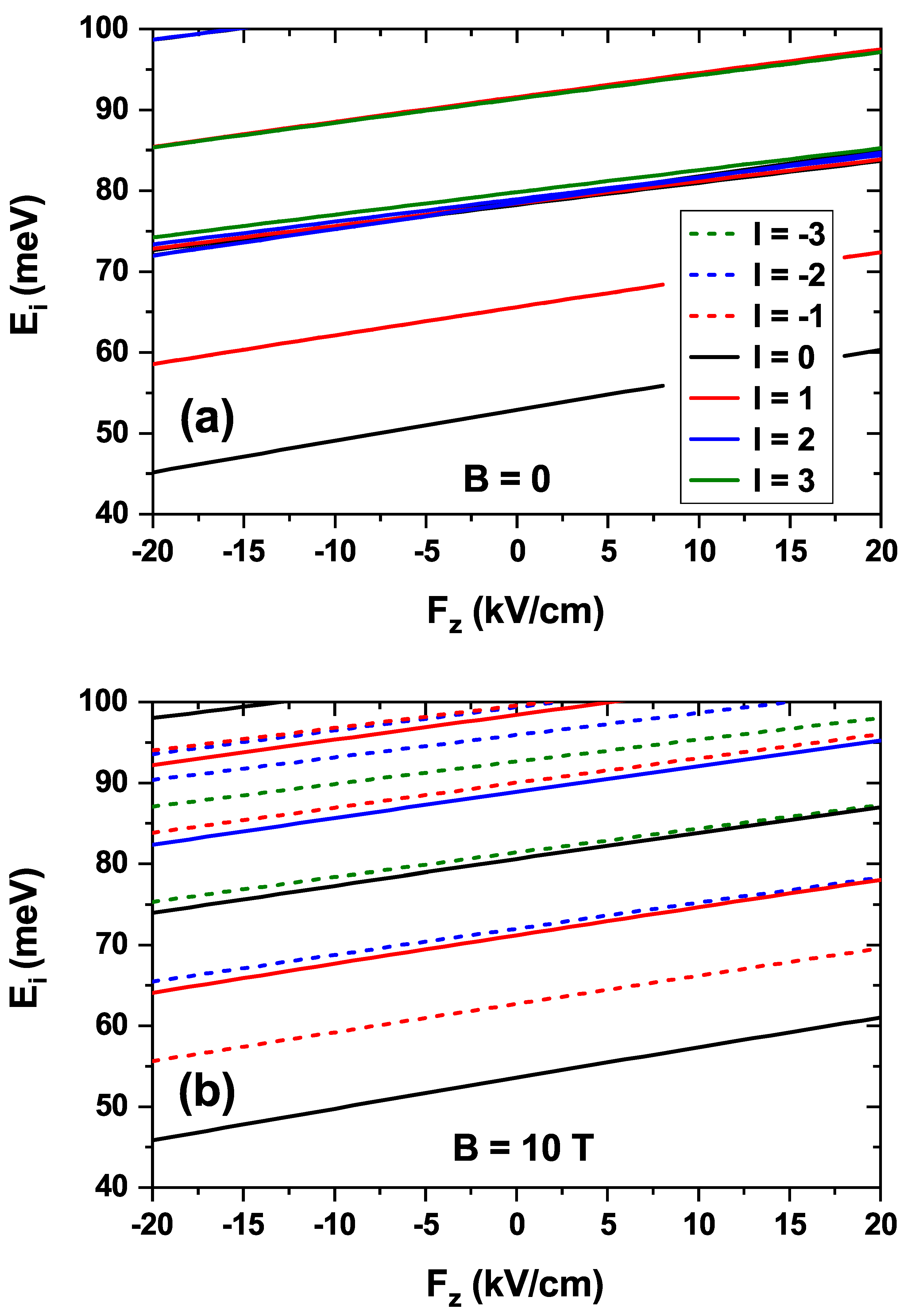
Figure 5.
Energy spectrum as a function of the magnetic field intensity for different values of the quantum number l. The calculations correspond to zero electric field (a) and kV/cm (c). A zoom of the gray-highlighted energy region in (a) and (c) for magnetic field values between 0 and 2 T is also presented in panels (b) and (d), respectively. In all cases, the magnetic field is applied along the positive z-direction.
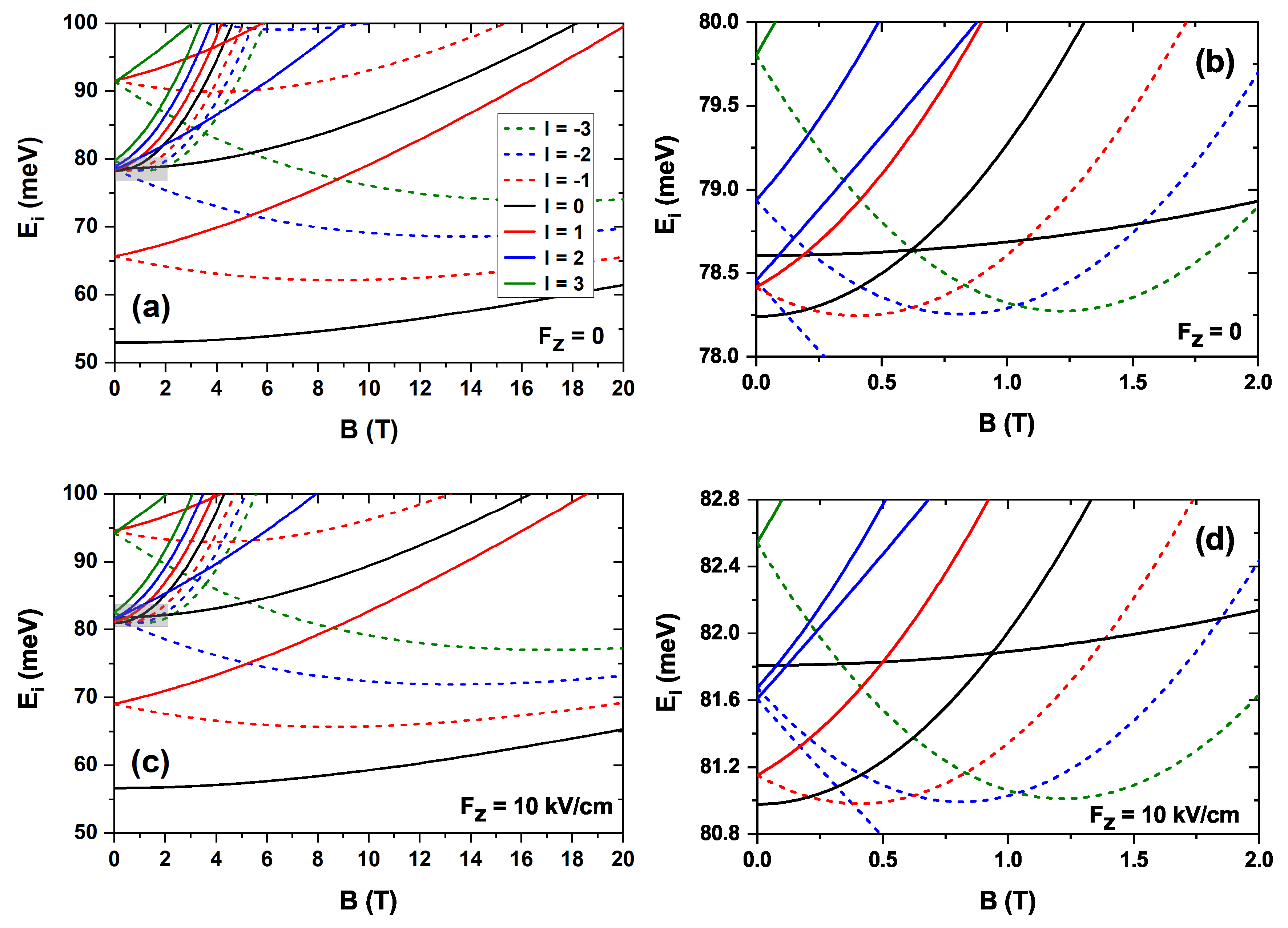
Figure 6.
Energy spectrum as a function of the magnetic field intensity for different values of the quantum number l as a result of the decomposition of the complete structure in the quantum dot (a) and the quantum ring (b). The superposition of the results shown in (a) and (b) is shown in panel (c). A schematic representation of the nanostructures is shown in (d). The calculations correspond to a zero electric field. In all cases, the magnetic field is applied along the positive z-direction.
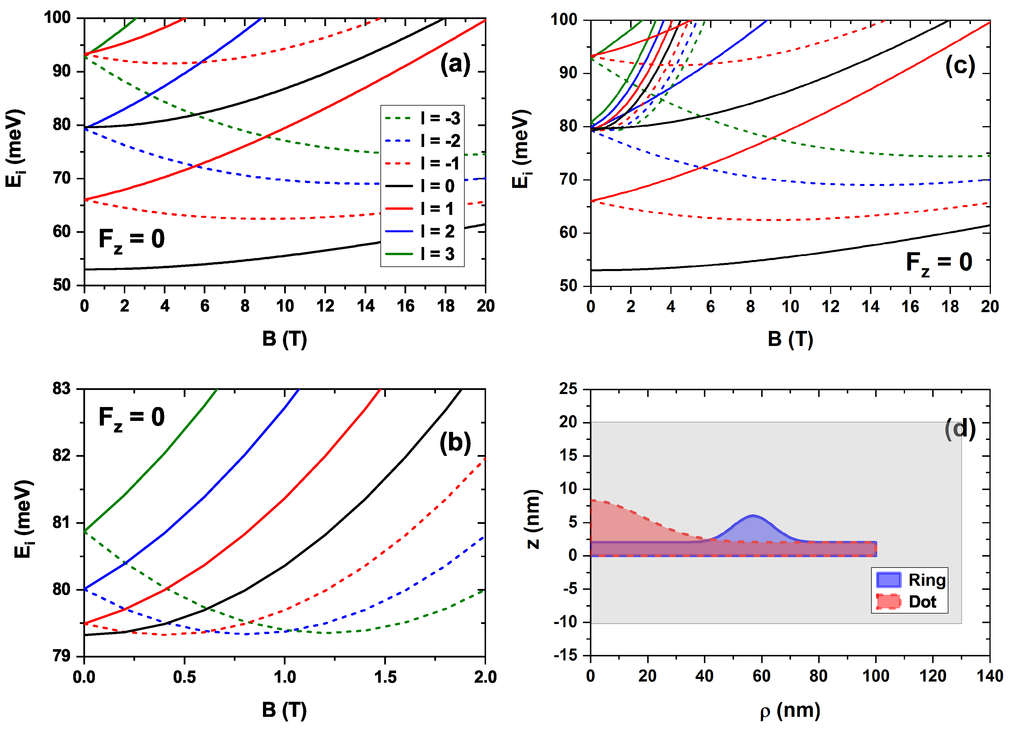
Figure 7.
Electromagnetically induced transparency (solid lines) in the ladder configuration associated with the first three energy levels for three different values of the electric field with zero magnetic field (a) and T (b) as a function of the probe field energy. The corresponding values of the linear absorption coefficient in terms of the incident-photon energy are represented by the shaded regions. For visualization, the absorption curves have been divided by 3. In all cases, the magnetic field is applied along the positive z-direction.

Figure 8.
Squared absolute value of reduced () electric dipole moments involved in the calculation of the electromagnetically induced transparency, and for zero magnetic field (a) and under the effect of a T magnetic field (b), as functions of the externally applied electric field . The values correspond to the ground (1) and first two excited (2, 3) states and are obtained for linearly polarized light in the z-direction. The magnetic field is applied along the z-direction.
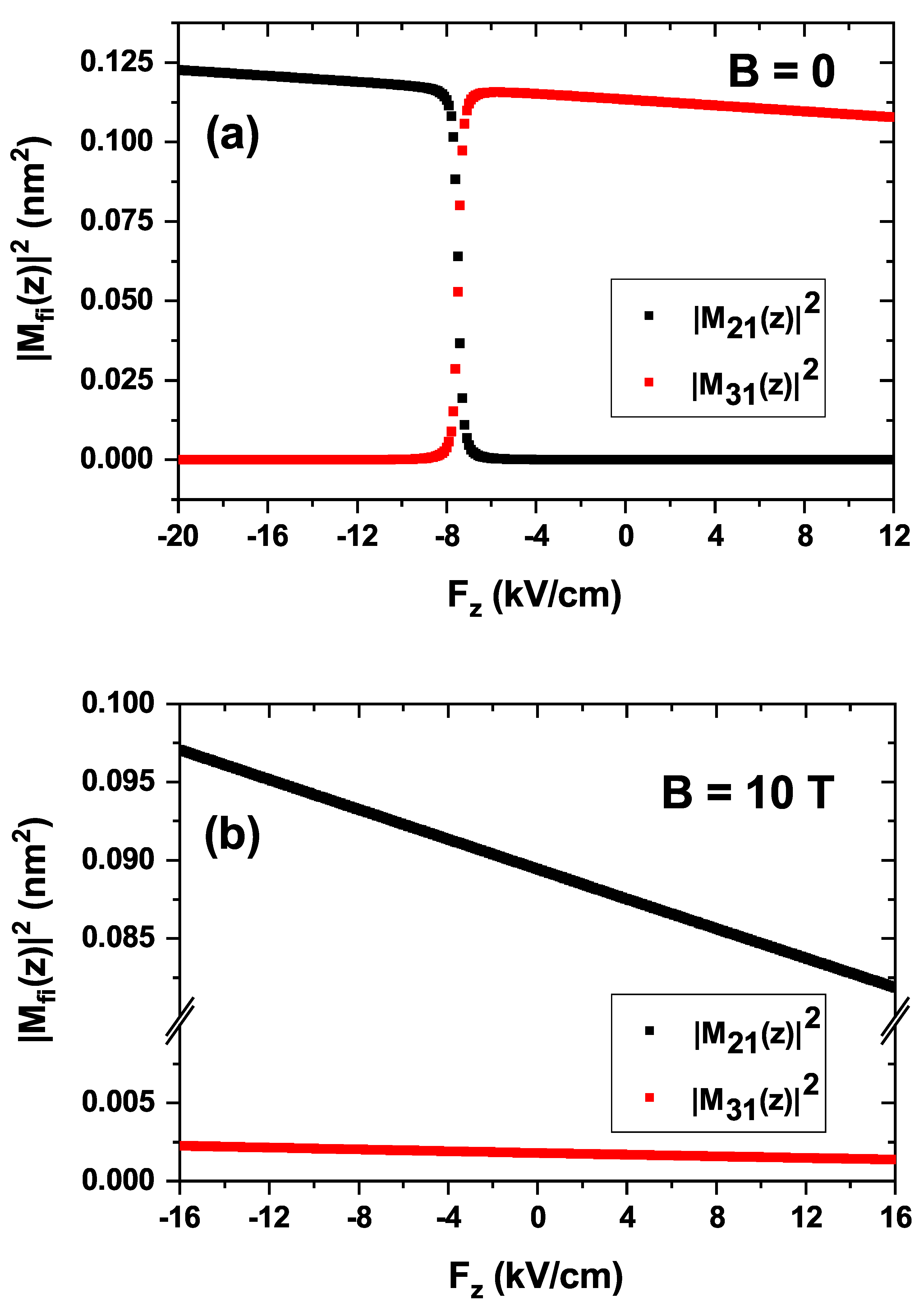
Figure 9.
Energy of the first three states (, , and ) as a function of the applied electric field F, calculated for (a) a zero magnetic field (B = 0 T) and (b) a magnetic field of B = 10 T. Note that a dominant linear component has been subtracted from the plotted energy values to emphasize the non-linear Stark effect. The gray shaded areas correspond to the electric field values used in Figure 7.

Figure 10.
Electromagnetically induced transparency in the cascade configuration and the corresponding values of the linear absorption coefficient associated with the three first energy levels for three different values of the magnetic field with zero electric field (a) and kV/cm (b) in terms of the incident photon energy. In all cases, the magnetic field is applied along the positive z-direction.
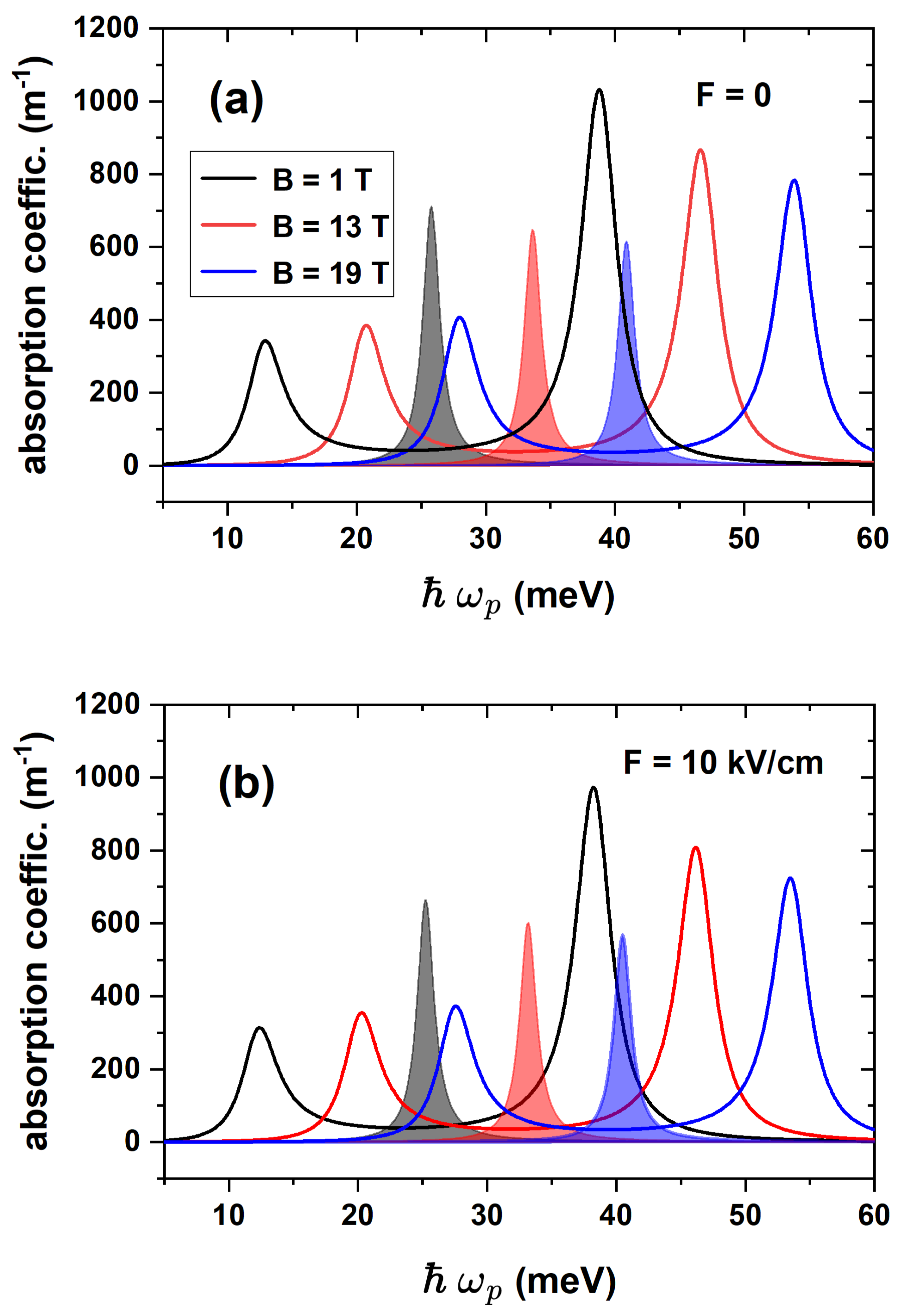
Figure 11.
Squared electric dipole matrix elements, , as a function of the applied magnetic field B. The figure shows the elements for the transitions from the ground state () to the first two excited states, (black) and (red). Solid lines correspond to a zero electric field (), while dashed lines represent the results under an external electric field of kV/cm. Calculations assume linearly polarized light along the z-direction.
Disclaimer/Publisher’s Note: The statements, opinions and data contained in all publications are solely those of the individual author(s) and contributor(s) and not of MDPI and/or the editor(s). MDPI and/or the editor(s) disclaim responsibility for any injury to people or property resulting from any ideas, methods, instructions or products referred to in the content. |
© 2025 by the authors. Licensee MDPI, Basel, Switzerland. This article is an open access article distributed under the terms and conditions of the Creative Commons Attribution (CC BY) license (http://creativecommons.org/licenses/by/4.0/).
Copyright: This open access article is published under a Creative Commons CC BY 4.0 license, which permit the free download, distribution, and reuse, provided that the author and preprint are cited in any reuse.


