
Submitted:
07 August 2025
Posted:
08 August 2025
You are already at the latest version
Abstract
Red blood cell (RBC) morphology is critical for diagnosing hematological disorders, particularly in regions such as Southeast Asia where anemia and thalassemia are highly prevalent. However, manual microscopic assessment is labor-intensive, subjective, and dependent on expert availability, while existing automated methods often rely on small, curated datasets that fail to represent real-world smear variability. This study proposes a hybrid framework integrating preprocessing, unsupervised autoencoding, k-means clustering, ellipse fitting, expert-in-the-loop validation, and targeted data augmentation to establish a robust RBC labeling pipeline. High-resolution smear images from confirmed anemia and thalassemia cases were processed to extract over 14,000 single-cell patches, filtered systematically into quality-assured subsets. Latent features from a CNN autoencoder enabled clustering into 80 morphological groups, quantified using ellipse-based geometric metrics and validated by hematology experts. Data augmentation addressed class imbalance, expanding rare morphologies while preserving realistic cell structure. The resulting dataset captures clinically relevant morphological diversity specific to the Thai population and provides a scalable, interpretable framework for medical analysis and future AI model development in hematology.
Keywords:
red blood cell morphology
; autoencoder
; ellipse fitting
; unsupervised clustering
; data augmentation
; anemia
; thalassemia
1. Introduction
RBC morphology plays a vital role in the diagnosis of various hematological disorders, including thalassemia, iron deficiency anemia, and hemolytic diseases [1,2]. In clinical practice, this morphological assessment traditionally relies on manual microscopic examination of peripheral blood smears by experienced hematologists. This process, while effective, is time-consuming, prone to human error, and inherently subjective [3]. These challenges are especially critical in low-resource settings such as Southeast Asia, where the burden of inherited hemoglobinopathies—particularly thalassemia—is notably high, and access to expert hematologists remains limited. For instance, in Thailand—a country with one of the highest thalassemia burdens in Southeast Asia—carrier rates are estimated at 30–40% of the population, particularly in the northern and northeastern regions. HbE carriers alone account for over 52% with a mortality rate of 1.13 per 100,000 individuals. These figures underscore the urgent need for scalable [12,13,14,15].
Recent advances in computer vision and deep learning have enabled significant progress in automating RBC classification tasks [4,5]. However, most existing models are trained and evaluated on datasets collected predominantly from Western populations (e.g., U.S., Europe) [6,7], whose blood smear characteristics—such as cell size, staining patterns, and prevalence of morphological abnormalities—differ considerably from those in Southeast Asian patients. This discrepancy introduces potential performance bias when such models are deployed cross-regionally. Moreover, widely used public datasets such as ALL-IDB [9], Rezatofighi, S.H. [2], Buczkowski, M. [10], and BCCD [11] have facilitated benchmarking in RBC classification research. However, they exhibit critical limitations that hinder their applicability in real-world clinical settings. These datasets are typically curated under ideal laboratory conditions—containing well-separated, uniformly stained cells—and rarely include real-world artifacts such as overlapping cells, uneven staining, or background debris. Additionally, they are modest in scale—usually fewer than 10,000 labeled cells—and insufficient for training robust models for complex use cases [8]. Furthermore, public RBC datasets often lack key technical variations—such as differences in microscope type, staining protocol, magnification, and scanner settings—leading to poor model generalization across clinical environments. This “technical reality gap” hinders reliable deployment in settings with diverse imaging conditions. Moreover, most models trained on these datasets are not clinically validated or interpretable, as they lack expert oversight. In low-resource settings, the absence of an expert-in-the-loop mechanism further reduces trust and usability, especially when the training data fails to reflect local morphological patterns. These limitations underscore the importance of frameworks that combine automation with human validation.
To address the limitations of existing RBC annotation approaches, we propose a novel hybrid pipeline that integrates geometric analysis, unsupervised deep learning, and expert-in-the-loop verification. The process begins with the extraction of high-resolution blood smear images in SVS format, scanned from real patient samples. These digital slides are then reviewed to identify appropriate regions of interest (ROIs), which are manually cropped into rectangular patches based on visual quality and cell density. Each ROI is subdivided into uniformly sized subregions to isolate candidate single-cell areas. To capture morphological features without requiring manual labels, we evaluate two unsupervised learning architectures: convolutional neural networks and dense autoencoders. The latter is selected for its superior latent representation capability. Autoencoder-derived feature vectors are subsequently clustered using the k-means algorithm to group morphologically similar cells, functioning as a pre-labeling step for downstream analysis. To further characterize individual cells, ellipse fitting is applied to each candidate, enabling shape- and size-based discrimination. This quantitative description enhances the interpretability of cell morphology across clusters. Finally, to address class imbalance—particularly for rare abnormal morphologies such as teardrop, sickle, or fragmented cells—we employ a targeted data augmentation strategy based on deformable ellipse transformations, thereby enriching underrepresented classes with plausible synthetic variants. This study makes the following three key contributions:
- It presents a novel combination of shape-based segmentation and deep unsupervised learning for RBC morphology analysis, a pairing that remains underexplored in prior literature.
- It proposes a scalable annotation framework capable of generating clinically relevant pseudo-labels with minimal expert involvement, reducing annotation cost while enabling model generalization to underrepresented populations.
- It introduces one of the largest real-world abnormal RBC datasets to date, consisting of over 10,000 peripheral smear images and corresponding metadata from Thai patients, helping to bridge both geographic and morphological gaps in current datasets.
2. Related Works
2.1. Whole Slide Image Processing and ROI Extraction
In recent years, the use of whole-slide imaging (WSI) formats such as SVS format has become increasingly important in digital pathology workflows, enabling high-resolution scanning of entire blood smear slides for downstream computational analysis. However, many previous studies in RBC or WBC morphology classification have utilized cropped or pre-segmented images obtained under controlled conditions, often bypassing the challenges inherent in real-world smear interpretation [2,16]. These studies typically rely on fixed-field images or single-cell views without addressing how to navigate or extract diagnostically relevant regions from full WSI data. While a few works have explored automatic ROI selection using heuristic or random sampling methods [17], they lack adaptive strategies based on morphological density, cell aggregation, or diagnostic saliency—factors crucial for analyzing heterogeneous slides collected from clinical environments. Moreover, the absence of standardized protocols for ROI identification in large-scale smear datasets has limited reproducibility and model generalizability. Therefore, the integration of intelligent ROI selection in WSI analysis remains an underexplored yet essential component of scalable morphological annotation systems.
2.2. Single-Cell Extraction and Instance Separation
Accurate extraction of single RBCs from peripheral blood smear images remains a critical pre-processing step in morphology-based classification pipelines. Traditional methods for RBC segmentation often rely on thresholding, edge detection, and watershed algorithms [18]. While these methods are computationally efficient, they tend to struggle in the presence of touching or overlapping cells, resulting in under- or over-segmentation artifacts. To mitigate this, more recent approaches have incorporated deep learning techniques such as U-Net and Mask R-CNN, which enable instance-level segmentation with improved accuracy [19]. However, these models require extensive pixel-level annotations for training and often generalize poorly to real-world smear slides with noisy backgrounds, variable staining, and densely clustered cells. Furthermore, most studies do not enforce constraints on ROI size or uniformity during extraction, which can affect downstream morphological analysis. Despite these advances, the field still lacks a simple yet robust framework that can extract uniformly sized single-cell instances from real-world smear images in a scalable and generalizable manner.
2.3. Unsupervised Learning and Morphological Clustering
While supervised learning has dominated recent advances in RBC and WBC classification, the increasing cost and time required for manual annotation have driven growing interest in unsupervised and semi-supervised approaches. Autoencoders, in particular, have shown promise in capturing latent morphological representations of blood cells without requiring explicit labels [20]. These latent spaces can be clustered using algorithms such as k-means or DBSCAN to group morphologically similar cells, offering an alternative route to pseudo-label generation [21]. Despite their potential, most studies have focused on white blood cells (WBCs), and applications to abnormal RBC morphology—especially in real-world smears—remain limited. Furthermore, the comparison between different encoder backbones, such as CNNs versus fully connected (dense) autoencoders, has not been systematically explored in hematological image analysis. Such comparison is critical, as morphological cues in RBCs are often subtle and shape-dependent, and the optimal encoder architecture may vary based on image resolution, background noise, and dataset characteristics. Our work addresses this gap by evaluating both CNN and dense autoencoder models in the context of unsupervised RBC clustering from real Thai patient smears.
2.4. Shape-Based Modeling and Ellipse Fitting
Shape-based analysis has long been utilized in hematological image processing to quantify cellular morphology through geometric features such as area, perimeter, circularity, and eccentricity [22]. These hand-crafted descriptors provide interpretable and computationally inexpensive measures that are useful for distinguishing between normal and abnormal RBC types. However, they often fail to generalize when applied to real-world smears where cell boundaries are unclear or distorted due to touching or staining artifacts. To enhance shape-guided representation, several studies have explored advanced contour modeling techniques, including active contours and Hough transform-based ellipse detection [23,24]. Among these, ellipse fitting has shown promise in capturing the overall geometry of RBCs, which are inherently biconcave and approximately elliptical in healthy forms. Nonetheless, the integration of ellipse fitting into modern deep learning pipelines—particularly in the context of unsupervised representation learning—remains scarce. Few studies have treated the ellipse not merely as a post-hoc measurement, but as a structural prior to guide downstream feature extraction or clustering [25]. This gap presents an opportunity to revisit classical shape modeling within contemporary machine learning frameworks for robust morphological analysis.
2.5. Human-in-the-Loop Expert Refinement
Manual annotation by domain experts remains the gold standard in hematological image labeling; however, it is notoriously time-consuming and prone to inter-observer variability, particularly for abnormal RBC morphologies. To address this challenge, several recent studies have explored human-in-the-loop (HITL) frameworks, where experts iteratively refine or verify AI-generated outputs rather than annotating from scratch [26]. This approach has been shown to significantly reduce labeling effort while maintaining diagnostic reliability. In medical imaging domains such as histopathology, HITL strategies have improved both model accuracy and user trust through interactive feedback cycles [27,28]. Despite these advantages, the adoption of HITL in RBC morphology remains limited. Most existing studies focus either on supervised classification or post hoc validation, without integrating expert judgment during the unsupervised clustering or pseudo-label generation phase. Moreover, few systems offer intuitive interfaces that allow experts to filter, correct, or reassign morphological clusters efficiently [29]. Our study builds upon these insights by incorporating expert-guided refinement into the unsupervised annotation loop, enabling more efficient pseudo-label validation and improving the overall quality of the dataset for downstream training.
2.6. Data Balancing and Rare-Class Augmentation
Class imbalance remains a persistent challenge in medical image datasets, particularly in hematology, where rare abnormal RBC morphologies—such as teardrop cells, fragmented cells, or target cells—are often underrepresented. This imbalance can bias deep learning models toward majority classes, resulting in poor sensitivity for clinically critical but infrequent phenotypes [30]. Traditional approaches such as oversampling and SMOTE (Synthetic Minority Over-sampling Technique) have been adopted to alleviate this issue, but they are limited by their tendency to generate redundant or unrealistic samples [31]. More recent efforts have explored the use of generative models, including GANs (Generative Adversarial Networks), to synthesize realistic minority-class cell images [32]. While promising, many of these models lack shape constraints or morphological priors, which are crucial for preserving biologically plausible features in RBCs. Additionally, only a few studies have attempted to apply domain-specific transformations—such as deformable ellipse fitting—to simulate natural variation in cell size, eccentricity, and contour, particularly for data-starved classes [33]. These methods offer a more explainable and geometry-aware alternative to black-box generators.
2.7. Summary and Research Gap
In summary, prior research has contributed significantly to various components of RBC image analysis—ranging from WSI preprocessing, ROI selection, single-cell segmentation, to supervised classification. However, most existing pipelines address these tasks in isolation and are rarely integrated into a unified framework capable of handling the complexity of real-world smear slides. The underutilization of unsupervised learning for RBC morphology, limited incorporation of geometric priors such as ellipse fitting, lack of expert-in-the-loop refinement strategies, and inadequate methods for augmenting rare phenotypes collectively highlight the need for a more holistic approach. Our work addresses these gaps by proposing an end-to-end hybrid framework that combines shape-based segmentation, latent space clustering, expert-guided pseudo-label validation, and deformable augmentation. This integrated methodology is specifically designed for real-world abnormal RBC annotation and aims to facilitate large-scale, efficient, and biologically interpretable dataset generation for hematological AI applications.
3. Materials and Methods
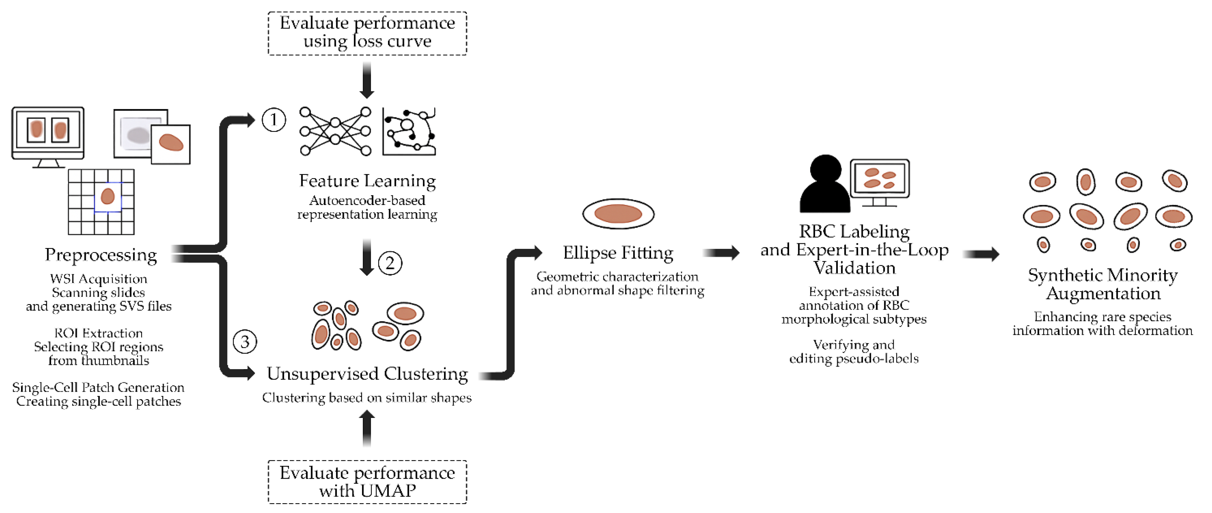
This study presents a multi-stage pipeline for the semi-automated annotation and morphological analysis of RBCs derived from digitized peripheral blood smear slides. The proposed workflow integrates WSI processing, unsupervised representation learning, shape-based priors, and expert-in-the-loop validation to address the challenges of manual annotation and data imbalance in hematological image analysis. The pipeline, illustrated in Figure 1, begins with the acquisition of high-resolution WSIs from clinically confirmed hematological cases (Section 3.1), followed by the extraction of diagnostically relevant ROIs (Section 3.2). From each ROI, uniformly sized single-cell patches are derived using a systematic grid sampling and filtering procedure (Section 3.3). Subsequently, latent morphological features are learned using autoencoder-based representation learning (Section 3.4) and clustered through unsupervised methods (Section 3.5) to group cells with similar appearances. To incorporate structural information, ellipse fitting is applied for geometric characterization and filtering of abnormal shapes (Section 3.6). The clustered results are then refined through expert-in-the-loop validation (Section 3.7), where hematology specialists confirm or adjust pseudo-labels. Finally, to address class imbalance among rare morphological subtypes, synthetic minority augmentation based on deformable ellipse transformations is performed (Section 3.8).
Figure 1.
Workflow of the proposed semi-automated RBC annotation and analysis pipeline.
3.1. Dataset Collection and Image Acquisition
This study utilized six WSIs of peripheral blood smears obtained from patients in Thailand with confirmed hematological diagnoses. The samples encompassed a range of anemic and thalassemic conditions: Sample ID 1: Iron Deficiency Anemia (IDA), Sample ID 2: Thalassemia Trait (TT), Sample ID 3: Hb H Disease (HbH), Sample ID 4: Thalassemia Hb E Disease (HbE/β-thal), Sample ID 5: Thalassemia Hb E Disease with Severe Symptoms (HbE/β-thal Sx), and Sample ID 6: Homozygous Hb E Thalassemia (Homo HbE). All diagnoses were clinically confirmed by hematologists based on standard laboratory tests and microscopic examination prior to slide preparation. No additional demographic or clinical data were collected in accordance with ethical guidelines for de-identification and patient privacy protection [34]. Blood smears were prepared following standard hematology protocols and stained using the Wright–Giemsa technique to enhance RBC morphology visualization [35]. The slides were digitized using a WSI scanner at 40× magnification, producing high-resolution digital slides in SVS format as shown in Figure 2(a). The scanning resolution was set to 0.1658 µm/pixel, providing sufficient detail for subsequent single-cell segmentation and morphological analysis [36]. Each WSI covered the entire smear area and served as the primary image source for all downstream experiments.
3.2. ROI Selection from WSI
From each WSI, two ROIs were manually selected by an expert hematologist, resulting in a total of 12 ROIs across the six slides. These ROIs were subsequently divided into two datasets for downstream experiments. The ROI dimensions were not fixed, as they were determined adaptively based on the distribution and density of RBCs in diagnostically relevant areas identified by the expert. Selection criteria for ROIs included (i) areas containing well-spread red blood cells without significant clumping or overlap, (ii) regions free from staining artifacts, debris, or scanning errors, and (iii) areas representative of typical morphological patterns for the corresponding hematological diagnosis [37]. These criteria ensured that ROIs captured diagnostically informative cells while minimizing noise as shown in Figure 2(b). ROIs were annotated using expert-driven selection and extracted automatically via the OpenSlide library to guarantee precise coordinate mapping and accurate image cropping from native-resolution WSIs [38]. All ROIs were retained at the original scanning resolution and subsequently downsampled only during visualization or model input preparation. Each ROI underwent independent review by a hematology expert to confirm diagnostic relevance. The extracted ROIs were stored in PNG format, preserving high-quality, lossless images suitable for computational analysis.
3.3. Single-Cell Patch Extraction
A total of 12 ROIs selected from WSIs were processed to extract single-cell patches of RBCs for downstream analysis. Cell detection was performed using a segmentation-based approach incorporating global thresholding, contour detection, and morphological operations. Segmentation masks were generated and refined using the watershed algorithm [39] to separate individual cells from touching clusters. For each segmented cell, a bounding box was derived from the binary mask and cropped to create a single-cell patch. To ensure accurate identification of isolated cells versus touching cells, a maximum local peak detection method was applied to centroid distributions within clusters [40]. Validated single-cell patches were overlaid on a clean background and centered to standardize positioning. Patches were saved in PNG format with a structured directory system separating: (i) single isolated cells, (ii) overlapping cells, (iii) broken or artifact cells, (iv) background or staining artifacts, (v) small particles, and (vi) cells touching image edges. This systematic organization facilitated both quality control and downstream dataset preparation [2]. The patch size for this study was set at 128 × 128 pixels, optimized for our ROI resolution (0.1658 µm/pixel) and compatibility with subsequent deep learning models. For other contexts, patch sizes can be adapted (e.g., 16, 32, 128, 256, or 512 pixels) depending on the desired field of view and computational constraints [41]. Filtering criteria were strictly applied to exclude: (i) overlapping cells, (ii) fragmented cells or artifacts, (iii) background regions or staining debris, (iv) small non-cellular particles, and (v) cells truncated at image edges. The detailed cell extraction process is visualized in Figure 3, while Algorithm 1 formally outlines the procedural steps, including segmentation, bounding box generation, artifact filtering, and patch centering.
| Algorithm 1. Pseudocode of the RBC single-cell extraction and resizing technique. |
| RBC_Extraction(image_path, output_dir) load image from image_path apply mean-shift filtering to image → shifted convert shifted image to grayscale → gray apply Otsu thresholding to gray → thresh find contours from thresh → cnts for each contour c in cnts do crop image and mask around contour → image_crop, mask_crop if mask_crop is valid then check if cell touches border: if true: save touching cell to "touching" folder else: extract RBC from mask determine RBC size: if size ≤ 16px: overlay to 32×32 and save as “small” else if size ≤ 32px: overlay to 32×32 and save as “32 size” else if size ≤ 128px: overlay to 128×128 and save as “128 size” else if size ≤ 256px: overlay to 256×256 and save as “256 size” else if size ≤ 512px: overlay to 512×512 and save as “512 size” else if size ≤ 1024px: overlay to 1024×1024 and save as “1024 size” else: save as "oversize" else: increment error_count number end for save processing results (original, filtered, gray, mask, contours) return success |
3.4. Latent Feature Learning Using Autoencoders
Latent morphological features of single-cell RBC patches were extracted using two encoder architectures: a dense autoencoder and a convolutional autoencoder (CNN-based). Both models were implemented using TensorFlow and Keras libraries [42], and their architectural diagrams are illustrated in Figure 4. Input cell patches (128 × 128 pixels, grayscale) were normalized to [0,1] before training. The dense autoencoder comprised a flattened input layer, a 64-unit latent layer with ReLU activation, followed by two decoding layers with sigmoid activation and reshaping back to the original size. The CNN-based autoencoder consisted of sequential convolutional and max-pooling layers for feature encoding, followed by mirrored upsampling and convolutional layers for reconstruction. Model training employed cross-validation, with 80% of the dataset used for training and 20% reserved for validation in each fold. Both models were trained for 200 epochs with a batch size of 64 on an NVIDIA GeForce RTX 1650 GPU. The binary cross-entropy loss function was used, and model performance was monitored using reconstruction loss as the primary metric [43]. Training histories were saved in CSV format, and loss curves were visualized to assess convergence. Encoders from both models were subsequently extracted for downstream unsupervised clustering tasks.
3.5. Unsupervised Clustering
The best-performing encoder selected from the autoencoder experiments (Section 3.4) was utilized to extract latent features of single-cell RBC images for clustering. These latent feature vectors were subsequently grouped using k-means clustering, implemented via the scikit-learn library [44]. The optimal number of clusters (k) was determined experimentally by iterative testing and qualitative expert evaluation, as no fixed ground truth labels were available. The quality of clustering was assessed primarily through expert visual review, wherein representative cell images from each cluster were inspected by a hematology specialist to verify morphological coherence within clusters [27]. To aid interpretation, the high-dimensional latent space was reduced to two dimensions using Uniform Manifold Approximation and Projection (UMAP) [45], enabling visualization of cluster separability and distribution patterns. The clustering process was conducted using TensorFlow (for latent feature generation) and scikit-learn (for clustering and evaluation). Resulting clusters were saved as image directories grouped by cluster ID to facilitate manual review and downstream analysis. Representative examples of clustered images were visualized to demonstrate intra-cluster similarity and inter-cluster distinctiveness. The detailed clustering procedure is summarized in Algorithm 2, which outlines the steps for latent feature extraction, cluster initialization, assignment, and qualitative validation.
| Algorithm 2. Unsupervised clustering of RBC latent features using k-means. |
| RBC_Clustering_Encoder(samples, encoder_models, n_clusters_list) for each sample_id in samples do initialize paths for model, images, and outputs create output folders if not exist load pre-trained encoder model for current sample_id load and preprocess RBC images → x_test normalize pixel values (0–1) encode images using encoder → encoded_imgs remove existing clustering score CSV if exists for each n_clusters in n_clusters_list do apply KMeans clustering (n_clusters) compute clustering labels → labels calculate Silhouette Score → sil_score calculate Davies-Bouldin Index → dbi_score save scores to CSV log create cluster folders and copy images based on labels plot silhouette visualization per cluster plot metrics comparison (Silhouette vs. DBI) save plots apply UMAP to reduce encoded_imgs to 2D plot and save UMAP scatter plot with cluster coloring save UMAP coordinates to CSV end for compile per-sample clustering report summarizing metrics and plots append results to global clustering summary (multi-sample CSV) end for compute total execution time and display summary return clustering results and diagnostic visualizations |
3.6. Morphological Prior via Ellipse Fitting
Ellipse fitting was applied to accurately quantify RBC morphology and provide shape-based priors for classification. The primary objectives were to (i) measure cell size precisely and (ii) evaluate shape characteristics such as circularity, ellipticity, and completeness, which are essential for distinguishing subtle morphological variations [46]. Ellipse fitting was implemented using edge-based contour fitting via the cv2.fitEllipse() function in OpenCV [47]. For each segmented cell, an ellipse was fitted to the contour, from which key morphological parameters were derived, including the major axis length (), minor axis length (), aspect ratio (AR), and ellipse-to-cell area ratio (ER). These were calculated as:
Cells with AR1 were considered circular, whereas higher AR values indicated elongation. The classify cell function (see Algorithm 3) applied threshold-based rules using AR, major axis length (µm), and ER to categorize cells into predefined groups (e.g., circular, oval, elongated) and filter out artifacts. Subsequently, morphological metrics were statistically analyzed, including AR for circularity, major axis length for RBC size standardization (6–8 µm), and ER to assess structural completeness [35]. This ensured that only morphologically valid cells were retained for downstream tasks. The full processing workflow, including contour detection, ellipse fitting, feature computation, and classification, is summarized in Algorithm 4, which automated morphological quantification while maintaining interpretability. This integration of geometry-based priors improved the reliability of subsequent clustering and annotation steps by removing irregular cells and enhancing feature quality.
| Algorithm 3. RBC Morphological classification based on geometric features. |
| classify_cell(ratio, length, area) if ratio ≤ 1.05: r_group = "Circle 095/" else if ratio ≤ 1.10: r_group = "Circle 090/" else if ratio ≤ 1.20: r_group = "Circle 080/" else if ratio ≤ 1.40: r_group = "Oval 060/" else if ratio ≤ 1.60: r_group = "Oval 040/" else: r_group = "Pencil/" if length < 6.0: l_group = "Micro/" else if length ≤ 8.0: l_group = "Normal/" else: l_group = "Macro/" if area ≤ 0.80: a_group = "Area 080/" else if area ≤ 0.90: a_group = "Area 090/" else if area ≤ 0.95: a_group = "Area 095/" else: a_group = "Area 100/" return concatenation of l_group, r_group, and a_group |
| Algorithm 4. Ellipse-based RBC Morphology classification and clustering. |
| RBC_Ellipse_Fitting_Clustering(data_list, image_path) for each folder in data_list do define folder_path if folder_path exists then for each image_file in folder_path do load image → image_input convert image to grayscale → gray apply Otsu thresholding → binary find contours from binary → contours for each contour cnt in contours do if contour length ≥ 5 then fit ellipse to contour → ellipse extract ellipse parameters: center, major_ax, minor_ax, angle compute major/minor axis lines and endpoints convert axis lengths to micrometers (µm) determine aspect ratio (AR) generate contour and ellipse masks compute overlap region (intersection) → inter_contours calculate area ratio (ER) annotate image with ellipse, axes, ratio, and area metrics classify cell morphology using classify_cell() function define output directories based on classification save annotated and raw images into their respective folders log extracted metrics for statistical analysis append classification results to CSV for later clustering review end for else: print warning (folder not found) end for export full metrics dataset and classification summary return morphological classification outputs and processed images |
3.7. Expert-in-the-Loop Validation
To ensure the reliability of the clustering results and improve pseudo-label quality, an expert-in-the-loop (HITL) validation process was implemented. Initially, RBC images were pre-classified based on the unsupervised clustering outputs and theoretical morphological guidelines, after which each cluster was reviewed and either approved or rejected by domain experts [48]. Two experts participated in this validation process: (i) an Associate Professor of Hematology specializing in medical training for physicians, and (ii) a Lecturer in Biomedical Physics with expertise in medical image analysis. Their complementary expertise allowed for both clinical and computational perspectives to be integrated into the review process. The experts followed specific validation criteria, including: (i) verifying the correctness of cluster labels based on RBC morphology, and (ii) approving or rejecting pseudo-labels for their suitability in subsequent training phases. During this process, representative samples from each cluster were inspected to confirm morphological coherence or identify misclassified or noisy samples. This validation was conducted over two refinement cycles, where feedback from each round was used to iteratively update the pseudo-label assignments and refine cluster integrity. This iterative HITL approach significantly improved label quality and reduced error propagation in subsequent model training, serving as a bridge between automated clustering and clinically robust annotation standards [49].
3.8. Synthetic Minority Augmentation
To address the issue of class imbalance, data augmentation was applied to increase the representation of rare morphological subtypes of RBCs. Imbalanced datasets are a well-known challenge in medical imaging, as they often bias model training towards majority classes and degrade performance in clinically important but underrepresented categories [30]. Synthetic samples were generated using controlled geometric transformations to preserve biological plausibility. Specifically, transformations were limited to rotation, flipping, and scaling down, ensuring that augmented data remained consistent with the original morphology and did not introduce unrealistic variations [50]. For each rare class, synthetic samples were generated at three scales: 1,000, 2,000, and 4,000 images per class, resulting in a more balanced training distribution. Augmentation operations were implemented in Python using OpenCV, NumPy, and SciPy libraries [47]. The workflow is described in Algorithm 5, which details the sequential application of resizing, rotation, and flipping, followed by dataset reorganization and saving augmented images. The effect of augmentation was evaluated by comparing model performance before and after augmentation, consistent with prior studies demonstrating that augmentation significantly improves classification accuracy in hematological imaging tasks [24,51]. These studies showed that class-balancing augmentation enhances sensitivity to rare morphological types and stabilizes learning curves, leading to improved generalization.
| Algorithm 5. Automated data augmentation and centering for RBC image dataset. |
| Auto_Data_Augmentation(data_list, image_path) for each folder in data_list do define folder_path if folder_path exists then for each image_file in folder_path do load image for each scale_factor in [0.98, 0.99, 1.00, 1.01] do resize image while embedding onto black background save augmented image for each rotation angle based on num_rotations do rotate resized image for each flip_code in [0, 1, -1] do flip rotated image (vertical, horizontal, both) else: Print warning (folder not found) end for for each folder in data_list do define folder_aug for each image_file in folder_aug do load augmented image → image apply mean-shift filtering → shifted convert to grayscale and apply Otsu thresholding → thresh detect contours → cnts for each contour c in cnts do extract ROI with small padding generate binary mask and apply bitwise extraction if extracted cell size < 128×128: embed cell into black 128×128 background, centered save centered image end for generate augmentation report summarizing transformations applied return augmented dataset and metadata logs |
4. Results
4.1. Preprocessing Results
From the WSIs of six hematological conditions, ROIs were extracted and divided into two datasets, each comprising representative regions from all disease categories. The specific dimensions of each ROI are detailed in Appendix A, where selection was guided by hematology experts to ensure diagnostically relevant regions. The number of single-cell patches obtained from ROI extraction is summarized in Table 1 for dataset 1 and Table 2 for dataset 2, which show the distribution of cells across different categories for their respective datasets. Single-cell patches, representing isolated RBCs, WBCs, or PLTs of suitable size (128 × 128 px), formed the primary dataset for downstream classification. Additional categories were also identified during preprocessing. The Extracted cells category included small cell clusters of two or three cells that could be separated and morphologically identified but were excluded from this study. The Overlapping cells category consisted of larger overlapping cell clusters where individual cells could not be distinctly resolved, and thus these were discarded. The Small cells category comprised cell fragments and clear platelet regions; while fragments were excluded, PLTs were retained as part of the dataset due to their diagnostic relevance. The Touching edge category contained cells truncated by ROI boundaries, rendering them unsuitable for analysis, while the Other category represented miscellaneous contaminants, which were absent in this dataset. Figure 5 presents representative examples of each category, illustrating the diversity of cell appearances identified during preprocessing. Notably, across both sample sets, Single-cell patches accounted for the majority of valid data, with proportions ranging from 55% to 70%, followed by Extract (10–20%) and Overlap (8–15%), while Small and Touching cells collectively contributed less than 10%. These results confirm that preprocessing effectively filtered unusable data and preserved diagnostically valuable single-cell patches for subsequent analysis.
4.2. Unsupervised Clustering Outcomes
After expert-guided filtering of single-cell patches, Dataset 1 contained 14,089 images, while Dataset 2 contained 11,496 images. These datasets were subsequently used to train both Dense Autoencoder and CNN Autoencoder models for unsupervised representation learning. The Dense Autoencoder model was trained on both datasets for 200 epochs, requiring approximately 1–1.5 hours per run. The minimum reconstruction loss values achieved were 6.44% and 6.55%, respectively, with stable convergence curves as shown in Figure 6(top). In comparison, the CNN Autoencoder model required a longer training duration of 7–8 hours for 200 epochs but yielded lower minimum loss values of 6.00% and 6.07%, respectively, with mildly fluctuating loss curves as illustrated in Figure 6(bottom). Overall, both models achieved acceptable reconstruction performance, with loss values ranging between 6.00–6.55%, supporting their suitability for unsupervised feature extraction. Given its superior accuracy, the CNN Autoencoder trained on Dataset 1 was selected for downstream clustering and annotation experiments. Nonetheless, the Dense Autoencoder remains advantageous for scenarios requiring faster training, reducing training time by up to fourfold while maintaining reasonable performance.
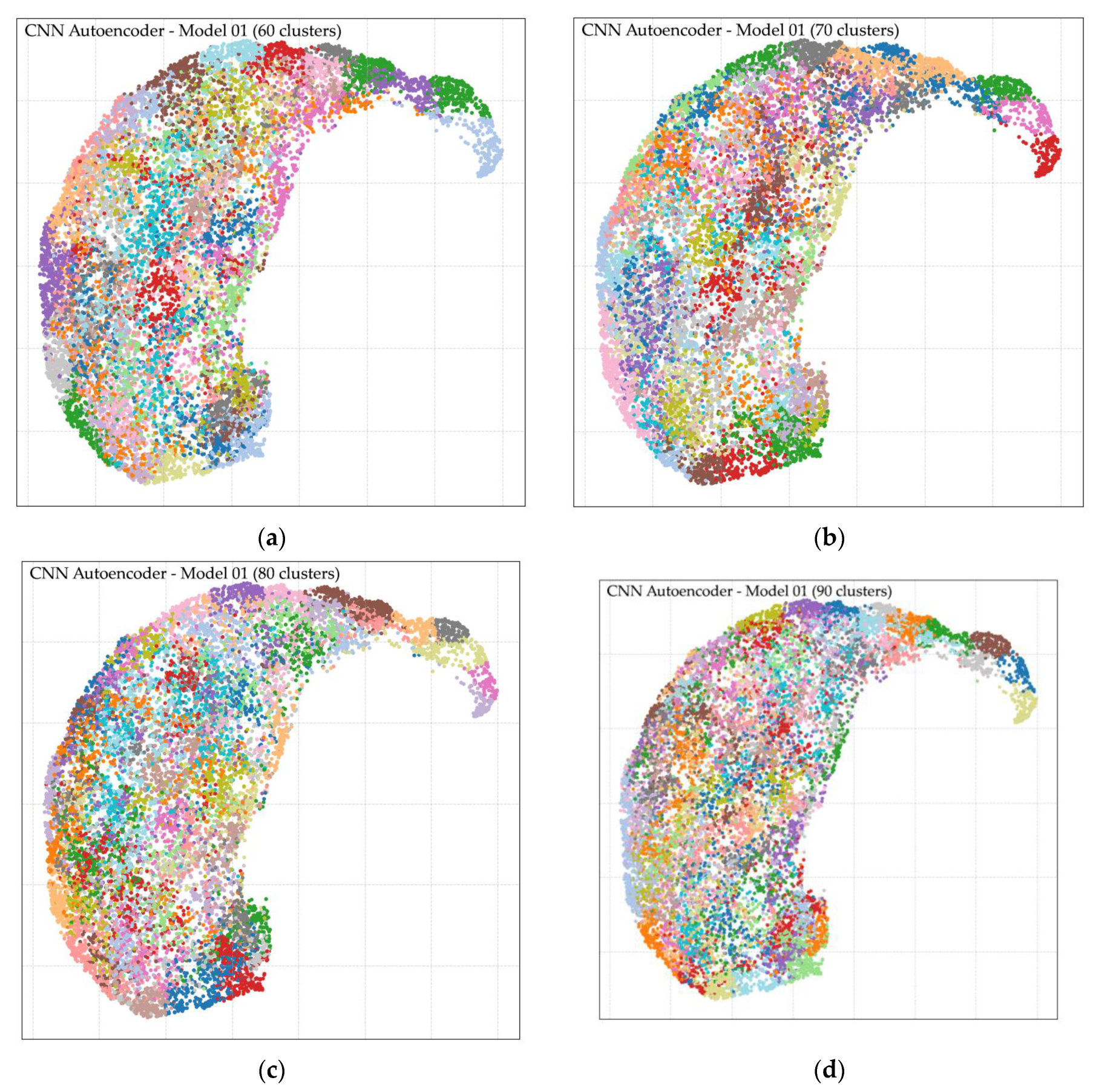
Following feature extraction using the CNN Autoencoder model trained on Dataset 1, unsupervised clustering was performed using k-means with varying numbers of clusters (k = 2, 3, 4, 5, 6, 7, 8, 9, 10, 20, 30, 40, 50, 60, 70, 80, 90, and 100). The analysis revealed that larger cluster counts, particularly in the range of k = 50 to k = 100, produced more distinct and morphologically coherent groupings compared to lower cluster counts. Cluster quality was evaluated through two complementary approaches: (i) direct expert review of representative cell images per cluster, and (ii) visual inspection of cluster separation in the UMAP-reduced latent space. Both methods confirmed improved intra-cluster homogeneity and inter-cluster separability at higher k values. The optimal result was achieved at k = 80, which yielded well-defined morphological clusters and clear separation in the UMAP visualization, as shown in Figure 7. Representative examples of clusters are provided in Appendix B, demonstrating distinct patterns grouped into their respective clusters. These findings indicate that clustering at k = 80 facilitates effective morphological grouping of RBCs and supports downstream classification. However, residual challenges remain in differentiating cell size, degree of elongation, and fine-grained shape variations, underscoring the need for the subsequent ellipse fitting-based size and shape analysis described in the next section.
4.3. Ellipse Fitting and Expert-Guided Labeling
Ellipse fitting was applied following k-means clustering, where the algorithm was programmed to automatically measure size and AR within each image folder corresponding to a cluster. This enabled systematic quantification of morphological features across all clustered cells. Cell circularity filtering was based on AR, evaluated at three thresholds: within ±5%, ±10%, and ±20% from perfect circularity. For oval cells, AR thresholds were relaxed to ±40%, ±60%, and ±80%, while cells exceeding ±80% AR were classified as pencil-shaped cells, indicative of extreme elongation. Cell size filtering was determined using the major axis length, categorized into three ranges: (i) < 6.00 µm for micro-sized cells, (ii) 6.00–8.00 µm representing normal-sized RBCs, and (iii) > 8.00 µm, which may also include larger cells such as WBCs within certain clusters. Additionally, ellipse-to-boundary ER was used to eliminate false fittings and incomplete cells. Multiple ER thresholds were applied sequentially (50%, 60%, 70%, 80%, 90%, 95%, and 100%), ensuring only cells with precise contour fits were retained for labeling. After applying these filters, the processed cells were separated into clearly organized folders for subsequent expert validation and labeling. Figure 8 provides representative examples of ellipse fitting outcomes, where AR and ER are annotated as R and A, respectively, for brevity. This figure illustrates the analysis stage only, while the images prepared for labeling were stored separately without annotations to maintain clean data for expert review.
After ellipse fitting, the data were pre-clustered into 80 groups without definitive RBC type labels. Using hematology references [52,53,54], clusters were classified into key RBC morphologies such as normocytes, Hypochromia, Howell-Jolly bodies, Codocyte (Target cell), Dacrocytes (Teardrop cell), Drepanocytes (Sickle cells), Eccentrocyte, Spherocyte, Stomatocyte, Ovalocytes, Elliptocytes, WBCs, PLTs, and others. Two hematology experts reviewed all clusters to validate morphological consistency and reassign labels where needed. The classification results for Dataset 1 are summarized in Table 3, while Figure 9 shows representative RBC morphologies, including normocytes, target cells, teardrop cells, and schistocytes. This expert validation ensured accurate labeling of all clusters, yielding a clinically reliable dataset for downstream analysis.
4.4. Data Augmentation
Data augmentation was applied using three controlled geometric transformations: scaling up and down (S), rotation (R), and flipping (F) to prevent unrealistic distortions of RBC morphology. These operations were iteratively executed in loops, producing a multiplicative increase in sample size with unique, non-redundant variations that enhanced dataset diversity. The augmentation process expanded each class to 1,000 and 4,000 images, depending on the target balance requirements. While augmentation could be performed on all available images, the selection of input images and applied transformations was adjusted systematically to achieve precise target counts, as detailed in Appendix C. Representative examples of augmented RBCs generated from scaling, rotation, and flipping are shown in Figure 10, demonstrating realistic morphological preservation while effectively increasing data diversity for training.
5. Discussion
RBC morphology is fundamental in diagnosing hematological disorders, particularly in regions such as Southeast Asia where thalassemia and anemia are highly prevalent. Traditional microscopic examination, while effective, is labor-intensive, subjective, and limited by the availability of trained hematologists. Moreover, existing automated approaches often rely on curated Western-centric datasets, which fail to capture the variability and artifacts present in real-world blood smears, reducing their generalizability. To address these challenges, we developed a hybrid framework integrating preprocessing, unsupervised autoencoding, ellipse fitting, expert-in-the-loop validation, and targeted data augmentation, aiming to produce a scalable, interpretable, and clinically relevant RBC labeling pipeline suitable for real-world diagnostic settings.
The preprocessing results demonstrated the effectiveness of our image processing approach in systematically isolating single-cell RBC images from high-resolution ROI samples. From the six ROI examples, the method successfully generated a substantial dataset, with Dataset 1 exceeding 10,000 single-cell patches across both datasets. The automated pipeline not only facilitated large-scale cell extraction but also implemented a structured filtering process that categorized cells into six groups. This systematic grouping significantly simplified expert review and ensured clear traceability of data quality. By removing noise such as overlapping clusters, edge-cut cells, and debris, the resulting dataset achieved a high level of purity, suitable for subsequent unsupervised clustering and morphological analysis. This preprocessing stage served as a crucial foundation, ensuring that downstream analysis operated on clean, standardized inputs rather than raw, artifact-laden smear images. Additionally, this preprocessing step provided insight into the distribution of cell artifacts and sample quality across ROI sources, which could inform further optimization of slide preparation and scanning protocols. For example, clusters of overlapping or edge-cut cells observed in specific ROIs highlight potential issues in smear spreading or scanner focus that may be addressed upstream. Overall, this 8preprocessing pipeline not only supports robust data preparation for computational modeling but also offers potential utility in improving hematology laboratory workflows by identifying sample preparation inconsistencies and guiding targeted quality control efforts.
The unsupervised clustering outcomes demonstrated the effectiveness of combining autoencoder-based feature extraction with k-means clustering for organizing RBC morphologies in an interpretable and scalable manner. After expert-guided filtering, Dataset 1 contained 14,089 images and Dataset 2 contained 11,496 images, forming a robust foundation for representation learning. Both Dense Autoencoder and CNN Autoencoder achieved reconstruction losses of 6.00–6.55%, consistent with studies indicating that low loss values reflect effective latent feature encoding [43,55]. While the Dense Autoencoder offered faster training with stable convergence, the CNN Autoencoder achieved lower loss despite requiring 7–8 hours, aligning with evidence that convolutional layers better preserve spatial detail for cellular imaging [56]. Thus, CNN Autoencoder from Dataset 1 was selected for clustering and annotation. Using its latent representations, k-means clustering was tested with k ranging from 2 to 100. Higher cluster counts, produced distinct and homogeneous clusters confirmed via expert review and UMAP visualization. The best result was at k = 80, yielding optimal intra-cluster consistency and inter-cluster separation, supporting findings that fine-grained clustering improves feature grouping in medical imaging [45,57]. These results confirm that unsupervised clustering can group RBC morphologies without labels, creating a strong basis for semi-automated annotation. Nonetheless, challenges remain in differentiating fine traits such as size, elongation, and borderline forms, emphasizing the need for ellipse fitting-based geometric analysis to refine classification precision. This approach bridges raw smear images with clinically interpretable clusters, enabling scalable pre-labeling for expert review.
Ellipse fitting was applied following k-means clustering to provide quantitative geometric measurements, enabling systematic filtering of cell size and shape. The algorithm automatically calculated AR, major axis length, and ER for each cluster, supporting objective evaluation of circularity and elongation. Cells were filtered into categories using AR thresholds (±5%, ±10%, ±20% for circularity; ±40%, ±60%, ±80% for ovality; >±80% for pencil shapes), size ranges (<6.00 µm for microcytes, 6.00–8.00 µm for normocytes, >8.00 µm for macrocytes or WBCs), and ER thresholds (50–100%) to exclude false fits and incomplete cells. The resulting cleaned images were organized into cluster folders for expert validation, as illustrated in Figure 8, where AR and ER are annotated as R and A for brevity. Following ellipse fitting, the pre-clustered data (80 groups) were reviewed against hematology standards [52,53,54]. Morphologies were classified into clinically recognized RBC types such as normocytes, hypochromic cells, codocytes (target cells), dacrocytes (teardrop cells), drepanocytes (sickle cells), spherocytes, elliptocytes, ovalocytes, as well as WBCs, PLTs, and others. Two hematology experts validated each cluster for morphological consistency and reassigned labels where needed. The classification results for Dataset 1 (Table 3) confirmed accurate distribution across 14,089 cells, with major categories including hypochromia (21.7%), spherocytes (20.9%), normocytes (5.8%), and rare forms like Howell-Jolly bodies (0.34%) and drepanocytes (0.18%). Representative morphologies are shown in Figure 9, illustrating clear visual differences between key cell types. This expert-guided review ensured that labeling was both clinically accurate and interpretable, establishing a reliable foundation for training and evaluation in downstream machine learning applications.
Data augmentation in this study was implemented through three controlled geometric transformations to preserve realistic RBC morphology while expanding dataset diversity. Iterative looping of these transformations produced unique, non-redundant samples and increased class sizes systematically. Depending on the target balance, augmentation expanded each class to 1,000 or 4,000 images, with representative examples shown in Figure 10. These results demonstrate that augmentation effectively increased data diversity while maintaining morphological integrity. Importantly, augmentation is not required for classes that already have sufficient image counts, as further expansion offers minimal added benefit. However, for rare or underrepresented classes, augmentation improved sample diversity and mitigated class imbalance—critical for robust training performance. In this study, lower representation of certain RBC morphologies was anticipated, as the dataset primarily focused on anemia and thalassemia cases, where disease-specific patterns inherently limited the presence of unrelated RBC types. Thus, data augmentation served as a targeted strategy to balance rare classes without introducing artificial distortions, ensuring that the dataset reflected realistic morphological variability while remaining aligned with the clinical spectrum of the study population.
This study demonstrates key strengths that advance RBC morphology research. First, we developed a hybrid framework combining preprocessing, unsupervised autoencoding, ellipse fitting, expert validation, and data augmentation, enabling scalable and clinically interpretable RBC labeling using real-world smear images from confirmed anemia and thalassemia cases, unlike prior studies reliant on small, curated datasets. Second, integrating ellipse fitting with expert-in-the-loop review balanced automation and clinical oversight, reducing annotation workload while ensuring accuracy by combining geometric quantification with hematologist expertise. Third, the use of unsupervised learning addressed limited labeled data in hematology, allowing effective pre-clustering before expert review. Together with augmentation for rare morphologies, the framework produced a large, high-quality labeled dataset suitable for AI development. Overall, this approach bridges computational modeling and clinical reality, supporting scalable RBC labeling and practical diagnostic relevance.
6. Conclusions
This study presents a hybrid framework for RBC labeling that integrates preprocessing, unsupervised autoencoding, ellipse fitting, expert validation, and targeted data augmentation, producing a clinically interpretable and scalable dataset derived from real-world smear images specific to Southeast Asia, where hematological profiles differ significantly from Western populations. These regional differences underscore the importance of context-specific datasets for both clinical analysis and AI training. Our framework not only supports automated and expert-guided RBC morphology assessment for medical diagnostics but also establishes a high-quality, well-annotated dataset suitable for future AI model development in hematology. Beyond its immediate application, this approach lays the groundwork for adaptable, data-driven pipelines that can be extended to other blood-related conditions, contributing to both clinical practice and computational medicine research.
7. Limitations and Future Work
This study has several limitations. First, ROI selection should be standardized and further investigated to determine the optimal size, which would allow for the analysis of the relationship between RBC density and disease-specific patterns. Second, clusters of touching cells were not separated into single cells; however, such groups may hold diagnostic significance in clinical hematology. Third, certain morphological classes such as Basophilic stippling, HbH inclusions, Diffuse basophilia, Cabot ring, Hb H, Hb C crystal, Hb SC crystal, Heinz bodies, Howell-Jolly bodies, Pappenheimer bodies, Keratocytes, and rare WBC subtypes (e.g., Basophil, Eosinophil, Lymphocyte, Monocyte, Neutrophil) were underrepresented or absent. While this does not affect our focus on anemia and thalassemia, a more comprehensive, region-specific dataset would enhance applicability across broader hematological disorders.
Future work will address these points by: (i) optimizing ROI selection and investigating RBC density correlations across disease types; (ii) segmenting touching (extracted) cells into single-cell images to evaluate their diagnostic contribution; (iii) expanding the dataset to include rare and underrepresented cell types for broader coverage; and (iv) studying RBC subtype distributions and standardized ratios for anemia and thalassemia cases within Thai populations to improve local relevance and clinical utility. In addition, future studies will explore the integration of advanced deep learning architectures, such as transformer-based models, to further enhance classification accuracy and interpretability. Furthermore, collaborative efforts with multiple regional hospitals will be pursued to create a larger, multi-institutional dataset that better reflects the variability of hematological profiles across Thailand.
Author Contributions
Conceptualization, B.A., S.W. and A.T.; methodology, B.A., S.W. and A.T.; software, B.A; validation, B.A., S.W. and A.T.; formal analysis, B.A., S.W. and A.T.; investigation, B.A., S.W. and A.T.; resources, S.W.; data curation, B.A.; writing—original draft preparation, B.A.; writing—review and editing, S.W. and A.T.; visualization, B.A.; supervision, S.W. and A.T.; project administration, B.A., S.W. and A.T.; funding acquisition, B.A., S.W. and A.T. All authors have read and agreed to the published version of the manuscript.
Funding
This research was funded by the Science Achievement Scholarship of Thailand (SAST). The APC was funded by the Science Achievement Scholarship of Thailand (SAST).
Institutional Review Board Statement
The study was conducted in accordance with the Declaration of Helsinki, and approved by the Institutional Review Board of Ubon Ratchathani University (protocol code UBU–REC–77/2568 and date of approval: 12 March 2025).
Informed Consent Statement
Informed consent was obtained from all subjects involved in the study. Written informed consent has been obtained from the patient(s) to publish this paper.
Data Availability Statement
The data supporting the reported results of this study are not publicly available due to privacy and ethical restrictions related to patient confidentiality. However, de-identified datasets may be made available from the corresponding author upon reasonable request and with appropriate ethical approval.
Acknowledgments
The authors would like to acknowledge the Faculty of Science, Ubon Ratchathani University, for providing administrative and technical support. We also thank the hematology laboratory staff for their assistance in sample preparation and provision of blood smear slides.
Conflicts of Interest
The authors declare no conflicts of interest. The funders had no role in the design of the study; in the collection, analyses, or interpretation of data; in the writing of the manuscript; or in the decision to publish the results.
Abbreviations
The following abbreviations are used in this manuscript:
| AI | Artificial Intelligence |
| AR | Aspect Ratio |
| CNN | Convolutional Neural Network |
| CSV | Comma-Separated Values |
| DBSCAN | Density-Based Spatial Clustering of Applications with Noise |
| ER | Ellipse-to-cell Area Ratio |
| F | Flipping |
| GAN | Generative Adversarial Network |
| GPU | Graphics Processing Unit |
| HbE | Thalassemia Hb E Disease |
| HbE Sx | Thalassemia Hb E Disease with Severe Symptoms |
| HbH | Hemoglobin H Disease |
| Ho HbE | Homozygous Hb E Thalassemia |
| HITL | Human-in-the-Loop |
| ID | Identifier |
| IDA | Iron Deficiency Anemia |
| k-means | K-means Clustering Algorithm |
| OpenCV | Open Source Computer Vision Library |
| PLT | Platelet |
| PNG | Portable Network Graphics |
| R | Rotation |
| RBC | Red Blood Cell |
| ReLU | Rectified Linear Unit |
| ROI | Region of Interest |
| S | Scaling up and down |
| SMOTE | Synthetic Minority Oversampling Technique |
| SVS | Scanned Virtual Slide Format |
| TT | Thalassemia Trait |
| UMAP | Uniform Manifold Approximation and Projection |
| U-Net | U-shaped Convolutional Neural Network |
| WBC | White Blood Cell |
| WSI | Whole Slide Image |
Appendix A
Appendix A.1
The study analyzed six WSIs in SVS format representing various hematological conditions: IDA, TT, HbH, HbE/β-thal, HbE/β-thal Sx, and Homo HbE. Each WSI was processed using Python with the OpenSlide library to extract essential metadata, including pixel size (0.1658 µm), magnification power (83×), number of image levels (4), and dimensions at the highest resolution. This metadata is critical for validating image quality and ensuring compatibility for downstream image processing tasks. In addition, thumbnails were generated and displayed for visual inspection, allowing verification of staining quality, smear uniformity, and potential artifacts, as illustrated in Figure A1. These thumbnails facilitated rapid screening prior to computational analysis, reducing the likelihood of processing flawed images. The extracted metadata and quality assessment outcomes are summarized in Table A1, which confirms consistency across all samples. This step ensured standardized, high-resolution inputs for subsequent preprocessing and provided a reliable baseline for comparing image characteristics across disease-specific samples. Moreover, this process demonstrates an effective workflow for digitizing and validating hematological slides, offering reproducible methodology for dataset preparation and serving as a reference for future large-scale RBC morphology studies.
Figure A1.
Example thumbnails of hematology samples derived from Whole Slide Image scans for different types of anemia and thalassemia, including (a) IDA, (b) TT, (c) HbH, (d) HbE/β-thal, (e) HbE/β-thal Sx, and (f) Homo HbE.
Figure A1.
Example thumbnails of hematology samples derived from Whole Slide Image scans for different types of anemia and thalassemia, including (a) IDA, (b) TT, (c) HbH, (d) HbE/β-thal, (e) HbE/β-thal Sx, and (f) Homo HbE.
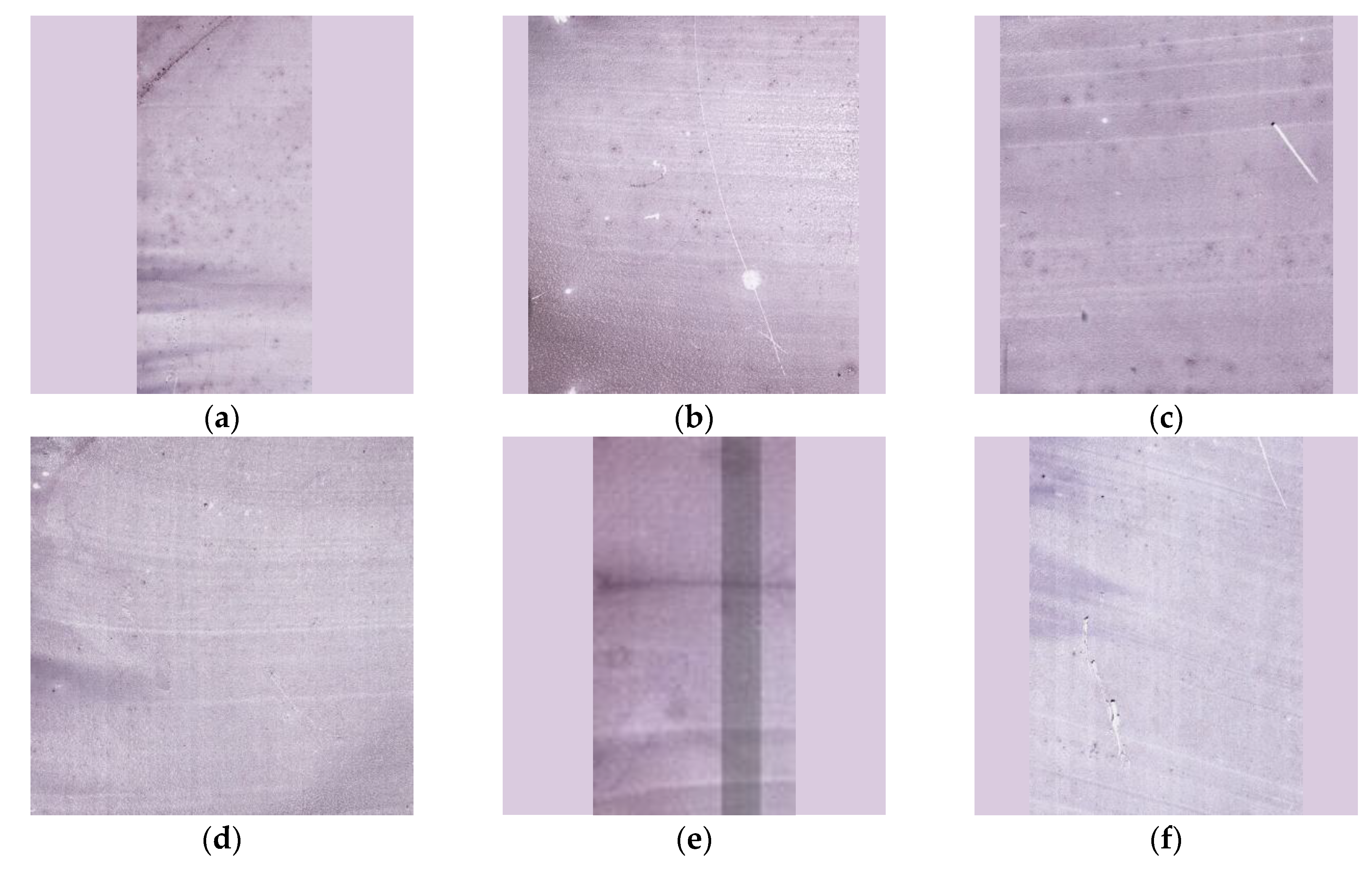

Table A1.
The extracted properties of pathology scanning slide.
| Sample Name | Pixel (µm) | Magnification | Levels | Dimensions (pixels) |
|---|---|---|---|---|
| IDA | 0.1658 | 83 | 4 | 34,271 x 74,047 |
| TT | 0.1658 | 83 | 4 | 44,743 x 51,260 |
| HbH | 0.1658 | 83 | 4 | 46,647 x 52,973 |
| HbE/β-thal | 0.1658 | 83 | 4 | 52,359 x 51,740 |
| HbE/β-thal Sx | 0.1658 | 83 | 4 | 39,031 x 73,061 |
| Homo HbE | 0.1658 | 83 | 4 | 39,983 x 55,429 |
Appendix A.2
Appendix A.2 illustrates examples of ROIs extracted from the six hematological samples, as shown in Figure A2, highlighting the representative areas selected for analysis based on cell density and image quality. Additionally, Table A2 summarizes the dimensions of the two ROIs extracted per sample, which were used to ensure coverage of diagnostically relevant areas while maintaining variability across datasets. This systematic ROI selection provided standardized inputs for subsequent preprocessing and feature extraction steps.
Figure A2.
Representative examples of ROI extractions from each sample WSI, selected based on diagnostic relevance and cell distribution, including (a) IDA, (b) TT, (c) HbH, (d) HbE/β-thal, (e) HbE/β-thal Sx, and (f) Homo HbE.
Figure A2.
Representative examples of ROI extractions from each sample WSI, selected based on diagnostic relevance and cell distribution, including (a) IDA, (b) TT, (c) HbH, (d) HbE/β-thal, (e) HbE/β-thal Sx, and (f) Homo HbE.
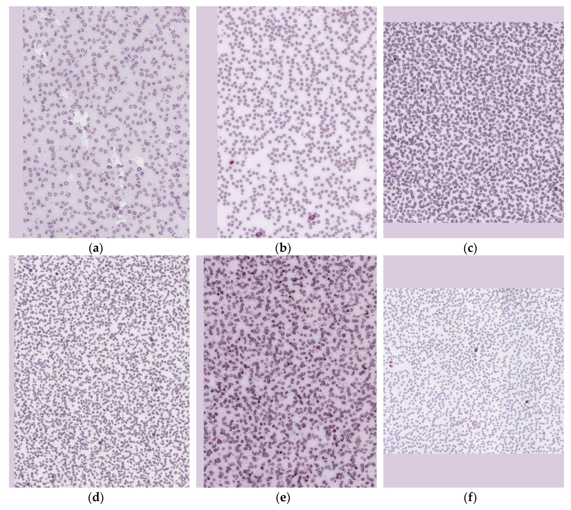
Table A2.
Dimensions of ROI 1 and ROI 2 (in pixels) for each sample analyzed in this study.
| Sample | Dimensions (pixels) | |
|---|---|---|
| ROI 1 | ROI 2 | |
| IDA | 2,358 x 2,882 | 2,489 x 2,751 |
| TT | 2,489 x 3,340 | 4,575 x 3,275 |
| HbH | 4,519 x 3,733 | 3,733 x 3,471 |
| HbE/β-thal | 7,991 x 4,454 | 4,454 x 5,043 |
| HbE/β-thal Sx | 3,144 x 5,305 | 3,013 x 3,471 |
| Homo HbE | 5,305 x 4,061 | 5,436 x 3,995 |
Appendix B
Appendix B presents the UMAP-based clustering analysis, as illustrated in Figure B1, showing visualizations for (a) 60 clusters, (b) 70 clusters, (c) 80 clusters, and (d) 90 clusters. It should be noted that repeated colors do not indicate identical cell morphologies but rather result from limited color assignments due to the high number of clusters; interpretation relies on the grouping of points. Highlighted areas in the figure demonstrate that the 80-cluster configuration achieved the clearest separation, providing balanced granularity for morphological grouping. However, both 70 and 90 clusters also yielded acceptable results: choosing 70 clusters reduces the number of clusters slightly but requires more expert work for verification, while choosing 90 clusters increases cluster detail but adds complexity. These findings support 80 clusters as an optimal choice for downstream labeling and morphological interpretation.
Figure 1.
UMAP visualization of RBC clustering at (a) 60 clusters, (b) 70 clusters, (c) 80 clusters, and (d) 90 clusters, with highlighted regions indicating clear morphological separations.
Figure 1.
UMAP visualization of RBC clustering at (a) 60 clusters, (b) 70 clusters, (c) 80 clusters, and (d) 90 clusters, with highlighted regions indicating clear morphological separations.
Appendix C
Appendix C presents the augmentation calculation Table C1, showing how input selection and transformation strategies were applied to achieve balanced output counts for each labeled RBC type. Although all labeled images could be used for augmentation, input selection was optimized to minimize redundancy and ensure computational efficiency, focusing on generating outputs that precisely meet the 1,000-image and 4,000-image targets. For example, rare classes such as Heinz bodies and Monocytes required high rotation multipliers (R) and scaling (S) to compensate for their low input counts, whereas abundant classes such as Spherocytes and Normocytes required fewer iterations. This demonstrates the principle of matching input-to-output ratios, where augmentation factors (e.g., R×F×S) are systematically adjusted to align with desired outputs.
Table 1.
The summarizes data augmentation techniques.
| Label list | Input | Augmentation | |
|---|---|---|---|
| 1,000 images | 4,000 images | ||
| Normocytes | 50 | R (5), F (3) | R (20), F (3) |
| Hypochromia +1 | 50 | R (5), F (3) | R (20), F (3) |
| Hypochromia +2 | 50 | R (5), F (3) | R (20), F (3) |
| Hypochromia +3 | 50 | R (5), F (3) | R (20), F (3) |
| Hypochromia +4 | 25 | R (10), F (3) | R (40), F (3) |
| Heinz bodies | 2 | R (125), F (3) | S (2), R (250), F (3) |
| Howell-Jolly bodies | 25 | R (10), F (3) | R (40), F (3) |
| Pappenheimer bodies | 10 | R (25), F (3) | R (100), F (3) |
| Codocytes - 01 | 250 | R (1), F (3) | R (4), F (3) |
| Codocytes - 02 | 250 | R (1), F (3) | R (4), F (3) |
| Eccentrocytes | 125 | R (2), F (3) | R (4), F (3) |
| Spherocytes - 01 | 250 | R (1), F (3) | R (4), F (3) |
| Spherocytes - 02 | 250 | R (1), F (3) | R (4), F (3) |
| Stomatocytes | 50 | R (5), F (3) | R (20), F (3) |
| Acanthocytes | 10 | R (25), F (3) | R (100), F (3) |
| Dacrocytes | 50 | R (5), F (3) | R (20), F (3) |
| Degmacytes | 25 | R (10), F (3) | R (40), F (3) |
| Drepanocytes | 25 | R (10), F (3) | R (40), F (3) |
| Echinocytes | 25 | R (10), F (3) | R (40), F (3) |
| Elliptocytes | 50 | R (5), F (3) | R (20), F (3) |
| Keratocytes | 5 | R (50), F (3) | R (200), F (3) |
| Knizocytes | 125 | R (2), F (3) | R (4), F (3) |
| Ovalocytes | 125 | R (2), F (3) | R (4), F (3) |
| Pyknocytes | 125 | R (2), F (3) | R (4), F (3) |
| Schistocytes | 125 | R (2), F (3) | R (4), F (3) |
| Lymphocyte | 25 | R (10), F (3) | R (40), F (3) |
| Monocyte | 2 | R (125), F (3) | S (2), R (250), F (3) |
| Neutrophil | 10 | R (25), F (3) | R (100), F (3) |
| Platelets - 01 | 50 | R (5), F (3) | R (20), F (3) |
| Platelets - 02 | 50 | R (5), F (3) | R (20), F (3) |
| Large - 01 | 250 | R (1), F (3) | R (4), F (3) |
| Large - 02 | 250 | R (1), F (3) | R (4), F (3) |
| Small | 50 | R (5), F (3) | R (20), F (3) |
| Other | 250 | R (1), F (3) | R (4), F (3) |
References
- Parab, M.A.; Mehendale, N.D. Red Blood Cell Classification Using Image Processing and CNN. SN COMPUT. SCI. 2021, 2, 70. [Google Scholar] [CrossRef]
- Rezatofighi, S.H.; Soltanian-Zadeh, H. Automatic Recognition of Five Types of White Blood Cells in Peripheral Blood. Comput. Med. Imaging Graph. 2011, 35, 333–343. [Google Scholar] [CrossRef] [PubMed]
- Fucharoen, S.; Winichagoon, P. Thalassemia in SouthEast Asia: Problems and Strategy for Prevention and Control. Southeast Asian J. Trop. Med. Public Health 1992, 23, 647–655. [Google Scholar] [PubMed]
- Shahzad, M.; Umar, A.I.; Shirazi, S.H.; Shaikh, I.A. Semantic Segmentation of Anaemic RBCs Using Multilevel Deep Convolutional Encoder-Decoder Network. IEEE Access 2021, 9, 161326–161341. [Google Scholar] [CrossRef]
- Afriyie, Y.; A. Weyori, B.; A.Opoku, A. Classification of Blood Cells Using Optimized Capsule Networks. Neural Process. Lett. 2022, 54, 4809–4828. [Google Scholar] [CrossRef]
- Alzubaidi, L.; Fadhel, M.A.; Al-Shamma, O.; Zhang, J.; Duan, Y. Deep Learning Models for Classification of Red Blood Cells in Microscopy Images to Aid in Sickle Cell Anemia Diagnosis. Electronics (Basel) 2020, 9, 427. [Google Scholar] [CrossRef]
- Khalid, U.; Gurung, J.; Doykov, M.; Kostov, G.; Hristov, B.; Uchikov, P.; Kraeva, M.; Kraev, K.; Doykov, D.; Doykova, K.; et al. Artificial Intelligence Algorithms and Their Current Role in the Identification and Comparison of Gleason Patterns in Prostate Cancer Histopathology: A Comprehensive Review. Diagnostics 2024, 14, 2127. [Google Scholar] [CrossRef]
- Sazak, H.; Kotan, M. Automated Blood Cell Detection and Classification in Microscopic Images Using YOLOv11 and Optimized Weights. Diagnostics 2025, 15, 22. [Google Scholar] [CrossRef]
- Labati, R.D.; Piuri, V.; Scotti, F. All-IDB: The Acute Lymphoblastic Leukemia Image Database for Image Processing. In Proceedings of the 2011 18th IEEE International Conference on Image Processing (ICIP), Brussels, Belgium, 11–14 September 2011; IEEE: New York, NY, USA, 2011; pp. 2045–2048. [Google Scholar]
- Buczkowski, M.; Szymkowski, P.; Saeed, K. Segmentation of Microscope Erythrocyte Images by CNN-Enhanced Algorithms. Sensors (Basel) 2021, 21, 1720. [Google Scholar] [CrossRef]
- Mohapatra, B. BCCD Dataset: Blood Cell Count and Detection. Kaggle Dataset Repository, 2015. Available online: https://www.kaggle.com/datasets/paultimothymooney/blood-cell-count-detection (accessed on 1 August 2025).
- Wasi, P.; Pootrakul, S.; Pootrakul, P.; Pravatmuang, P.; Winichagoon, P.; Fucharoen, S. Thalassemia in Thailand. Ann. N. Y. Acad. Sci. 1980, 344, 352–363. [Google Scholar] [CrossRef]
- V. Panich; M. Pornpatkul; and W. Sriroongrueng. The Problem of Thalassemia in Thailand. Southeast Asian J Trop Med Public Health 1992, 23 Suppl 2, 1–6.
- Teawtrakul, N.; Chansung, K.; Sirijerachai, C.; Wanitpongpun, C.; Thepsuthammarat, K. The Impact and Disease Burden of Thalassemia in Thailand: A Population-Based Study in 2010. J. Med. Assoc. Thai. 2012, 95 Suppl 7, S211–6. [Google Scholar]
- Paiboonsukwong, K.; Jopang, Y.; Winichagoon, P.; Fucharoen, S. Thalassemia in Thailand. Hemoglobin 2022, 46, 53–57. [Google Scholar] [CrossRef] [PubMed]
- Long, F.; Peng, J.-J.; Song, W.; Xia, X.; Sang, J. BloodCaps: A Capsule Network Based Model for the Multiclassification of Human Peripheral Blood Cells. Comput. Methods Programs Biomed. 2021, 202, 105972. [Google Scholar] [CrossRef] [PubMed]
- Zhong, A.; Li, X.; Wu, D.; Ren, H.; Kim, K.; Kim, Y.; Buch, V.; Neumark, N.; Bizzo, B.; Tak, W.Y.; et al. Deep Metric Learning-Based Image Retrieval System for Chest Radiograph and Its Clinical Applications in COVID-19. Med. Image Anal. 2021, 70, 101993. [Google Scholar] [CrossRef] [PubMed]
- Nurçin, F. V.; Imanov, E. Segmentation of Overlapping Red Blood Cells for Malaria Blood Smear Images by U-Net Architecture. J. Med. Imaging Health Inform 2021, 11, 2190–2193. [Google Scholar]
- Pfeil, J.; Nechyporenko, A.; Frohme, M.; Hufert, F. T.; Schulze, K. Examination of Blood Samples Using Deep Learning and Mobile Microscopy. BMC Bioinformatics 2022, 23, 65. [Google Scholar] [CrossRef]
- Dong, Z.; et al. scSemiAE: A Deep Model with Semi-Supervised Learning for Single-Cell RNA-Seq Data Analysis. BMC Bioinformatics 2022, 23, 439. [Google Scholar] [CrossRef]
- Ahmadzadeh, E.; Jaferzadeh, K.; Lee, J.; Moon, I. Automated three-dimensional morphology-based clustering of human erythrocytes with regular shapes: stomatocytes, discocytes, and echinocytes. J. Biomed. Opt. 2017, 22(7), 076015. [Google Scholar] [CrossRef]
- Yi, F.; Moon, I.; Javidi, B. Cell morphology-based classification of red blood cells using holographic imaging informatics. Biomed. Opt. Express 2016, 7(6), 2385–2399. [Google Scholar] [CrossRef]
- Ersoy, I.; Bunyak, F.; Higgins, J.M.; Palaniappan, K. Coupled Edge Profile Active Contours for Red Blood Cell Flow Analysis. In Proceedings of the 2012 9th IEEE International Symposium on Biomedical Imaging (ISBI); IEEE; 2012. [Google Scholar]
- Naruenatthanaset, K.; Chalidabhongse, T.H.; Palasuwan, D.; Anantrasirichai, N.; Palasuwan, A. Red Blood Cell Segmentation with Overlapping Cell Separation and Classification on Imbalanced Dataset. arXiv [eess.IV], 2020. [Google Scholar]
- Tofighi, M.; Guo, T.; Vanamala, J.K.P.; Monga, V. Deep Networks with Shape Priors for Nucleus Detection. In Proceedings of the 2018 25th IEEE International Conference on Image Processing (ICIP); IEEE; 2018. [Google Scholar]
- Budd, S.; Robinson, E. C.; Kainz, B. A Survey on Active Learning and Human-in-the-Loop Deep Learning for Medical Image Analysis. IEEE J. Biomed. Health Inform. 2021, 25, 2742–2756. [Google Scholar] [CrossRef]
- Holzinger, A.; Biemann, C.; Pattichis, C.S.; Kell, D.B. What Do We Need to Build Explainable AI Systems for the Medical Domain? arXiv [cs.AI].
- Tizhoosh, H.R.; Pantanowitz, L. Artificial Intelligence and Digital Pathology: Challenges and Opportunities. J. Pathol. Inform. 2018, 9, 38. [Google Scholar] [CrossRef]
- Foy, B.H.; Stefely, J.A.; Bendapudi, P.K.; Hasserjian, R.P.; Al-Samkari, H.; Louissaint, A.; Fitzpatrick, M.J.; Hutchison, B.; Mow, C.; Collins, J.; et al. Computer Vision Quantitation of Erythrocyte Shape Abnormalities Provides Diagnostic, Prognostic, and Mechanistic Insight. Blood Adv. 2023, 7, 4621–4630. [Google Scholar] [CrossRef]
- Johnson, J.M.; Khoshgoftaar, T.M. Survey on Deep Learning with Class Imbalance. J. Big Data 2019, 6. [Google Scholar] [CrossRef]
- Chawla, N.V.; Bowyer, K.W.; Hall, L.O.; Kegelmeyer, W.P. SMOTE: Synthetic Minority Over-Sampling Technique. J. Artif. Intell. Res. 2002, 16, 321–357. [Google Scholar] [CrossRef]
- Frid-Adar, M.; Klang, E.; Amitai, M.; Goldberger, J.; Greenspan, H. Synthetic Data Augmentation Using GAN for Improved Liver Lesion Classification. In Proceedings of the 2018 IEEE 15th International Symposium on Biomedical Imaging (ISBI 2018); IEEE; 2018. [Google Scholar]
- Rana, P.; Sowmya, A.; Meijering, E.; Song, Y. Data Augmentation with Improved Regularisation and Sampling for Imbalanced Blood Cell Image Classification. Sci. Rep. 2022, 12, 18101. [Google Scholar] [CrossRef] [PubMed]
- World Medical Association World Medical Association Declaration of Helsinki: Ethical Principles for Medical Research Involving Human Subjects: Ethical Principles for Medical Research Involving Human Subjects. JAMA 2013, 310, 2191–2194. [CrossRef] [PubMed]
- Bain, B.J. Blood Cells: A Practical Guide; 5th ed.; Wiley-Blackwell: Chichester, England, 2015. [Google Scholar]
- Erratum: Introduction to Digital Image Analysis in Whole-Slide Imaging: A White Paper from the Digital Pathology Association. J. Pathol. Inform. 2019, 10, 15. [CrossRef]
- Komura, D.; Ishikawa, S. Machine Learning Methods for Histopathological Image Analysis. Comput. Struct. Biotechnol. J. 2018, 16, 34–42. [Google Scholar] [CrossRef]
- Goode, A.; Gilbert, B.; Harkes, J.; Jukic, D.; Satyanarayanan, M. OpenSlide: A Vendor-Neutral Software Foundation for Digital Pathology. J. Pathol. Inform. 2013, 4, 27. [Google Scholar] [CrossRef]
- Beucher, S.; Meyer, F. The morphological approach to segmentation: The watershed transformation. Mathematical Morphology in Image Processing 1993, 34, 433–481. [Google Scholar]
- Vincent, L.; Soille, P. Watersheds in digital spaces: An efficient algorithm based on immersion simulations. IEEE Trans. Pattern Anal. Mach. Intell. 1991, 13, 583–598. [Google Scholar] [CrossRef]
- Sadafi, A.; Bordukova, M.; Makhro, A.; Navab, N.; Bogdanova, A.; Marr, C. RedTell: An AI Tool for Interpretable Analysis of Red Blood Cell Morphology. Front. Physiol. 2023, 14, 1058720. [Google Scholar] [CrossRef]
- Chollet, F. Deep Learning with Python; Manning Publications: Shelter Island, NY, USA, 2021. [Google Scholar]
- Goodfellow, I.; Bengio, Y.; Courville, A. Deep Learning; MIT Press: Cambridge, MA, USA, 2016. [Google Scholar]
- Pedregosa, F.; Varoquaux, G.; Gramfort, A.; Michel, V.; Thirion, B.; Grisel, O.; et al. Scikit-learn: Machine learning in Python. J. Mach. Learn. Res. 2011, 12, 2825–2830. [Google Scholar]
- McInnes, L.; Healy, J.; Melville, J. UMAP: Uniform Manifold Approximation and Projection for Dimension Reduction. arXiv [stat.ML], 2018. [Google Scholar]
- Gonzalez, R.C.; Woods, R.E. Digital Image Processing, 4th ed.; Pearson: New York, NY, USA, 2018. [Google Scholar]
- Bradski, G. The OpenCV Library. Dr. Dobb’s Journal of Software Tools 2000, 25, 120–126. [Google Scholar]
- Gupta, A.; Sabirsh, A.; Wahlby, C.; Sintorn, I.-M. SimSearch: A Human-in-the-Loop Learning Framework for Fast Detection of Regions of Interest in Microscopy Images. IEEE J. Biomed. Health Inform. 2022, 26, 4079–4089. [Google Scholar] [CrossRef]
- Holzinger, A.; Langs, G.; Denk, H.; Zatloukal, K.; Müller, H. Causability and Explainability of Artificial Intelligence in Medicine. Wiley Interdiscip. Rev. Data Min. Knowl. Discov. 2019, 9, e1312. [Google Scholar] [CrossRef]
- Shorten, C.; Khoshgoftaar, T.M. A Survey on Image Data Augmentation for Deep Learning. J. Big Data 2019, 6. [Google Scholar] [CrossRef]
- Xu, M.; Papageorgiou, D.P.; Abidi, S.Z.; Dao, M.; Karniadakis, G.E. A deep convolutional neural network for classification of red blood cells in sickle cell anemia. PLoS Comput. Biol. 2017, 13, e1005746. [Google Scholar] [CrossRef]
- Hatton, C.S.R.; Hughes-Jones, N.C.; et al. Lecture Notes: Haematology; 9th ed.; Wiley-Blackwell: New Jersey, USA, 2013. [Google Scholar]
- d’Onofrio, G.; Zini, G. Morphology of Blood Disorders; 2nd ed.; Translated by Bain, B.J.; Wiley-Blackwell: New Jersey, USA, 2014.
- Keohane, E.M.; Walenga, J.M.; Smith, L.J. Rodak’s Hematology: Clinical Principles and Applications; 5th ed.; Saunders: Philadelphia, PA, USA, 2015. [Google Scholar]
- Hinton, G.E.; Salakhutdinov, R.R. Reducing the Dimensionality of Data with Neural Networks. Science 2006, 313, 504–507. [Google Scholar] [CrossRef]
- LeCun, Y.; Bengio, Y. Convolutional networks for images, speech, and time series. Handbook of Brain Theory and Neural Networks 1995, 3361, 255–258. [Google Scholar]
- Esteva, A.; Kuprel, B.; Novoa, R.A.; Ko, J.; Swetter, S.M.; Blau, H.M.; Thrun, S. Dermatologist-Level Classification of Skin Cancer with Deep Neural Networks. Nature 2017, 542, 115–118. [Google Scholar] [CrossRef]
Figure 2.
Workflow of slide scanning and ROI selection using OpenSlide: (a) Glass slides were scanned with Aperio AT2. (b) ROIs were selected from SVS thumbnails.
Figure 2.
Workflow of slide scanning and ROI selection using OpenSlide: (a) Glass slides were scanned with Aperio AT2. (b) ROIs were selected from SVS thumbnails.
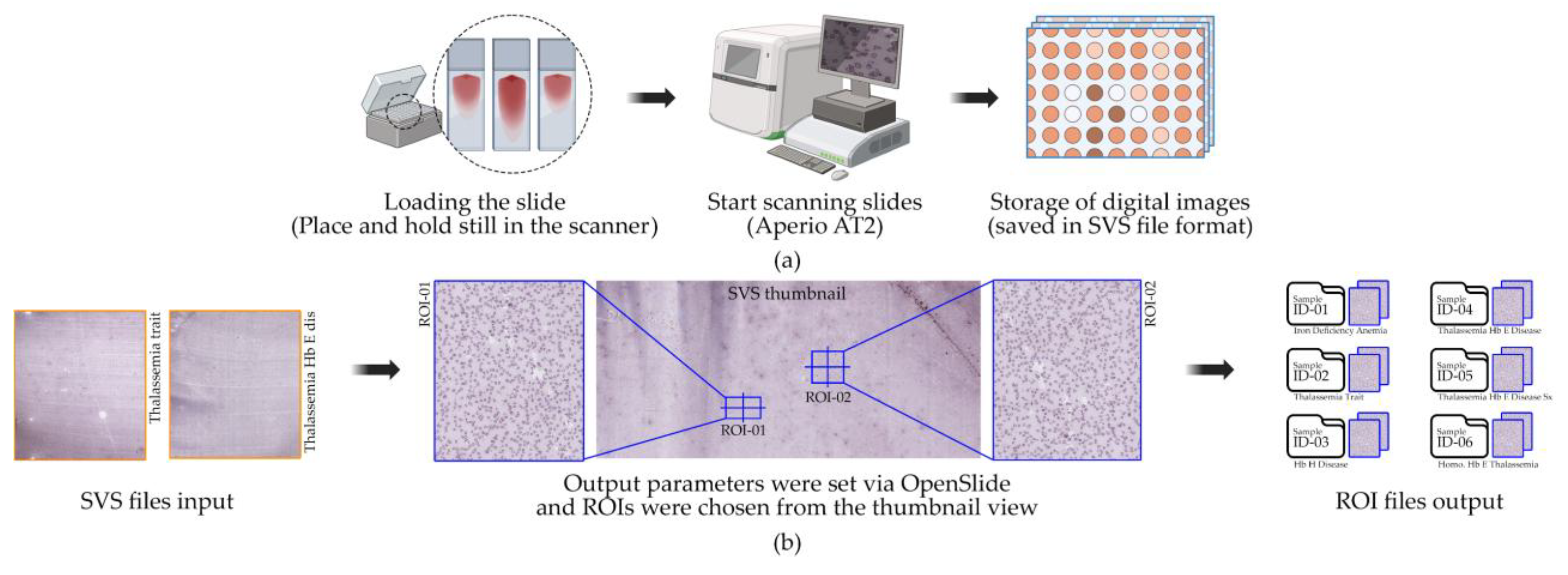
Figure 3.
Processing pipeline for single-cell patch extraction from ROIs. The figure illustrates the step-by-step workflow including segmentation, watershed-based separation, bounding box generation, artifact filtering, cell centering, and final patch export.
Figure 3.
Processing pipeline for single-cell patch extraction from ROIs. The figure illustrates the step-by-step workflow including segmentation, watershed-based separation, bounding box generation, artifact filtering, cell centering, and final patch export.
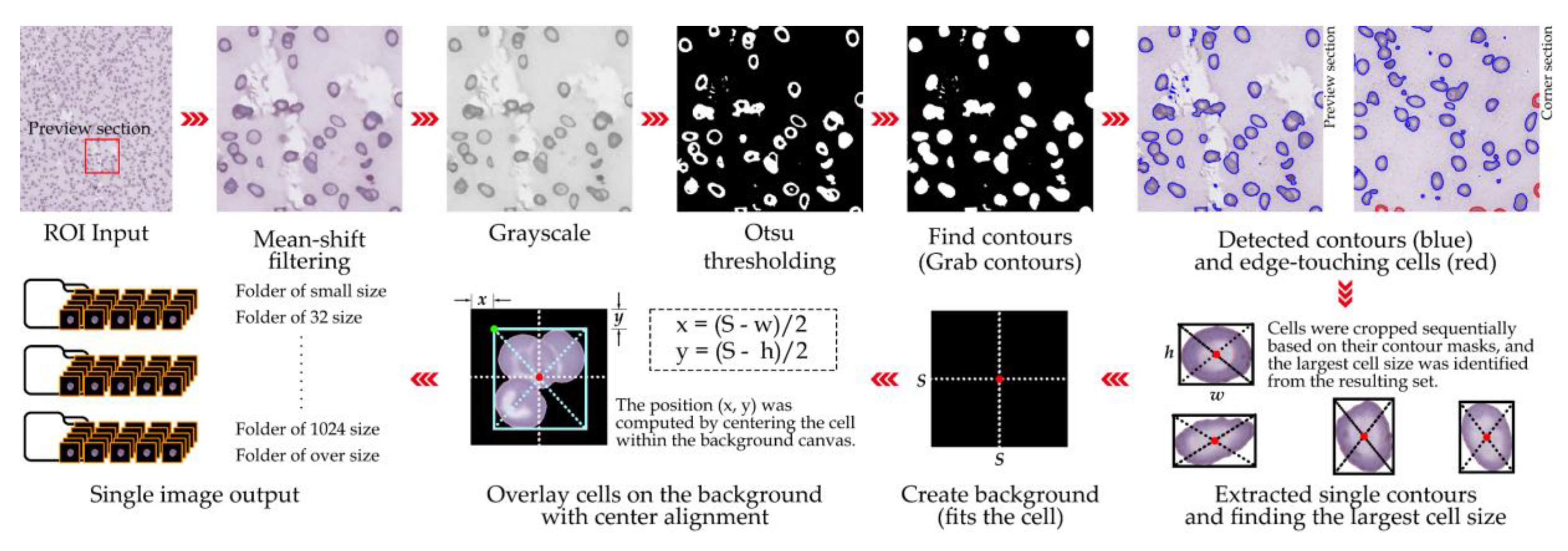
Figure 4.
Architectures for latent feature extraction: (a) dense and (b) CNN-based autoencoders.
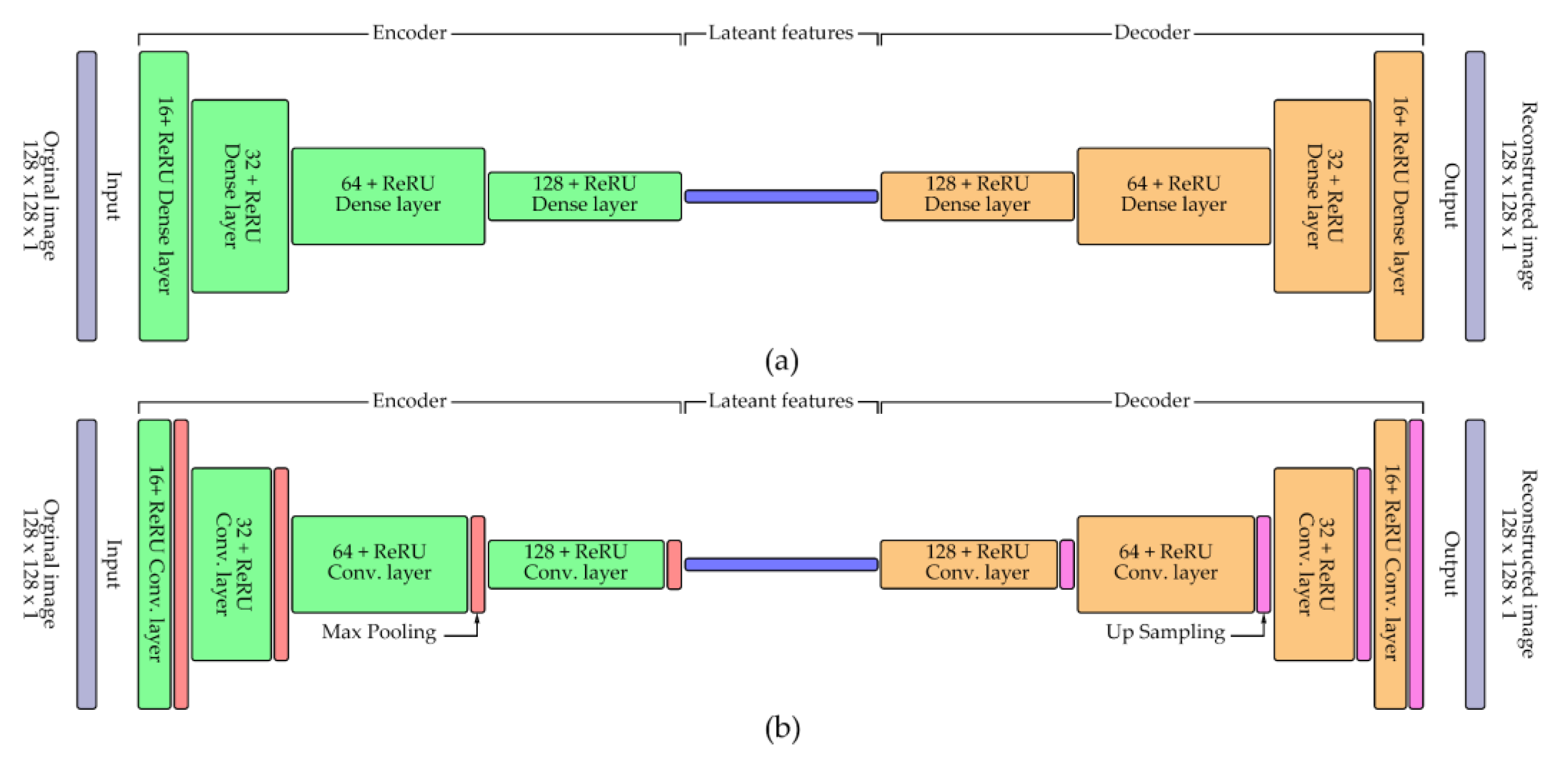
Figure 5.
Representative examples of cell categories identified during preprocessing: (a) Single cells; (b) Extracted cells; (c) Overlapping cells; (d) Small; and (e) Touching edge.
Figure 5.
Representative examples of cell categories identified during preprocessing: (a) Single cells; (b) Extracted cells; (c) Overlapping cells; (d) Small; and (e) Touching edge.
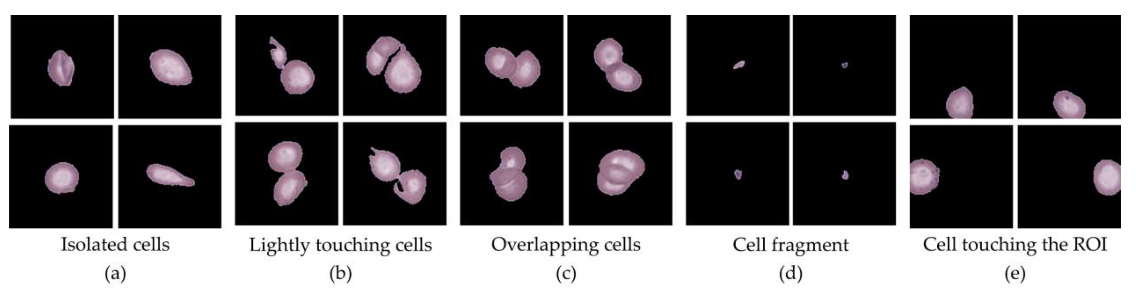
Figure 6.
Training loss curves over 200 epochs of (top) the Dense Autoencoder model; and (bottom) the CNN Autoencoder model.
Figure 6.
Training loss curves over 200 epochs of (top) the Dense Autoencoder model; and (bottom) the CNN Autoencoder model.
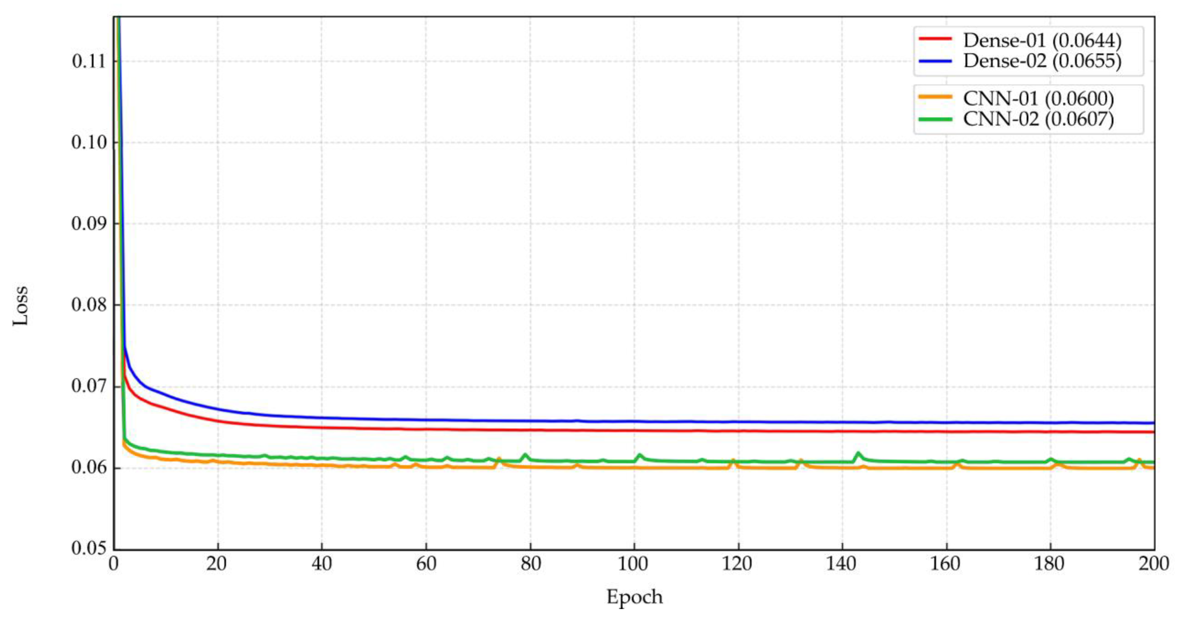
Figure 7.
UMAP visualization of clustered RBC latent features at k = 80, showing clear inter-cluster separation and intra-cluster homogeneity.
Figure 7.
UMAP visualization of clustered RBC latent features at k = 80, showing clear inter-cluster separation and intra-cluster homogeneity.
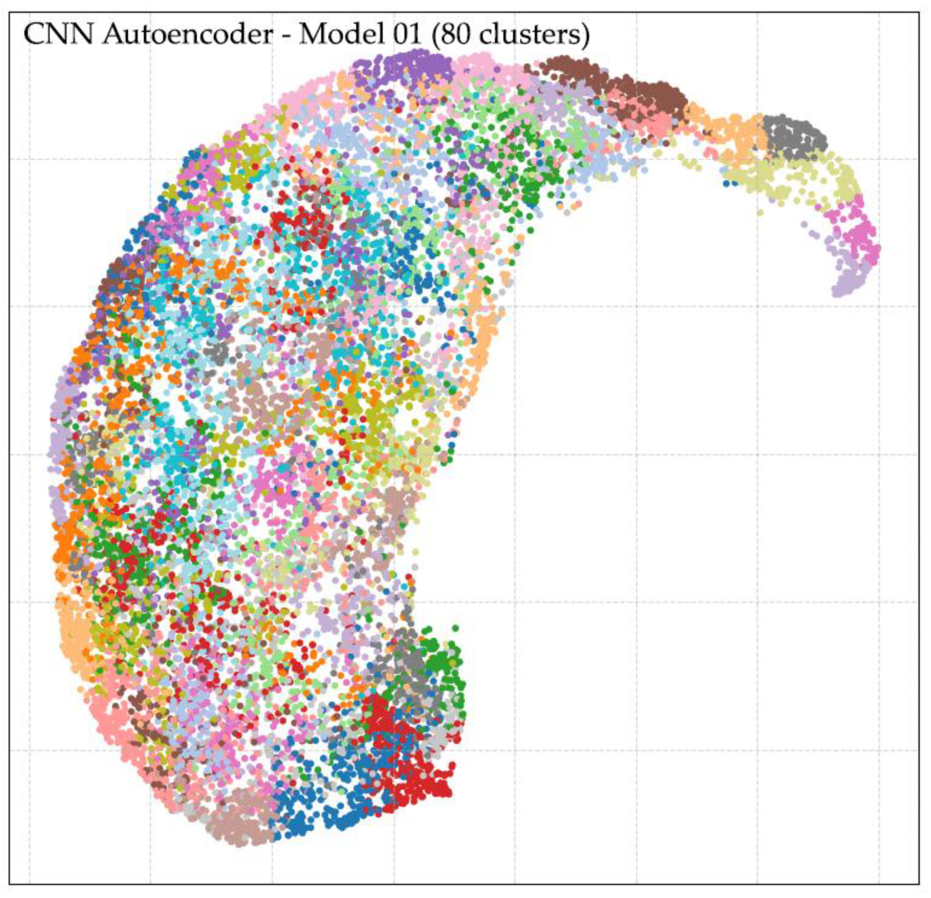
Figure 8.
Representative examples of ellipse fitting results showing annotated AR (R) and ER (A) values for RBCs across clusters. These images illustrate the analytical stage only, while clean images for labeling were stored separately.
Figure 8.
Representative examples of ellipse fitting results showing annotated AR (R) and ER (A) values for RBCs across clusters. These images illustrate the analytical stage only, while clean images for labeling were stored separately.
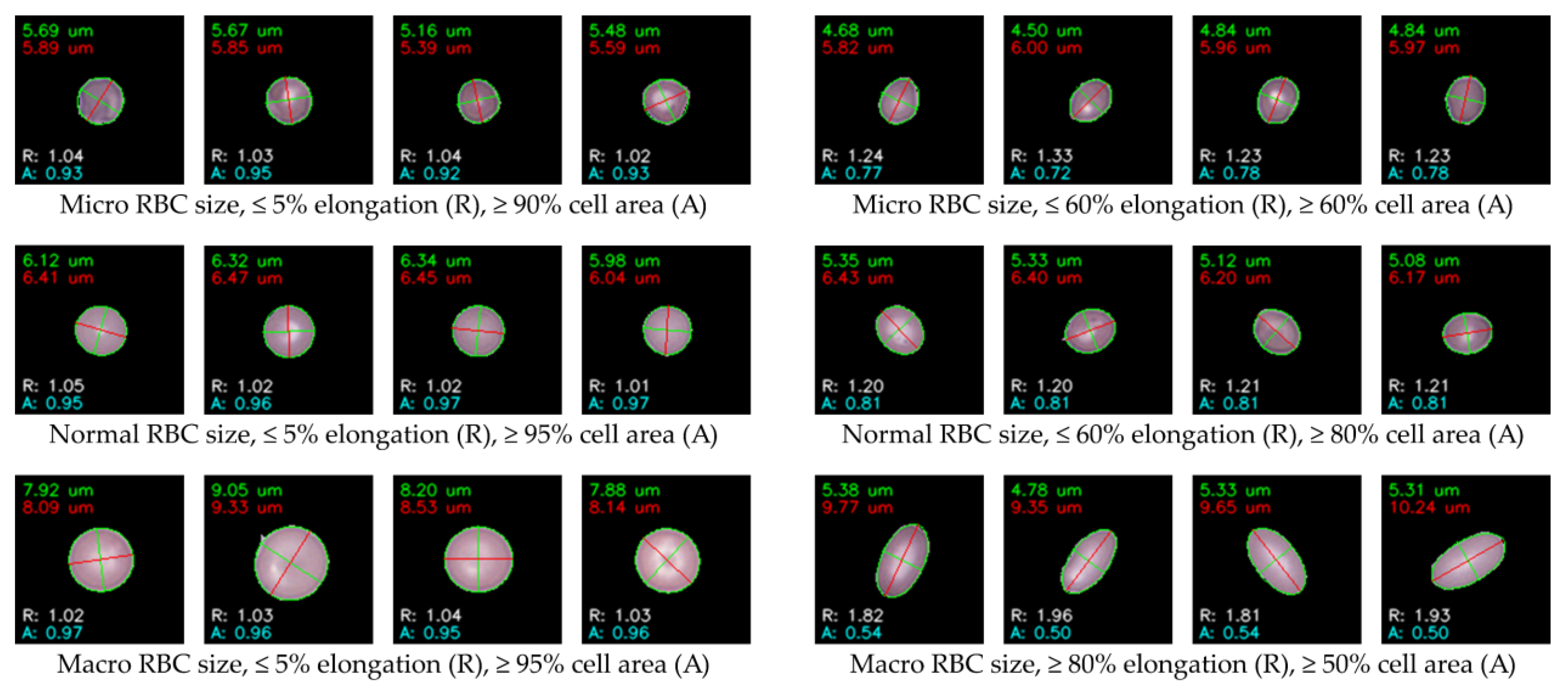
Figure 9.
Representative examples of RBC morphologies confirmed by expert review.
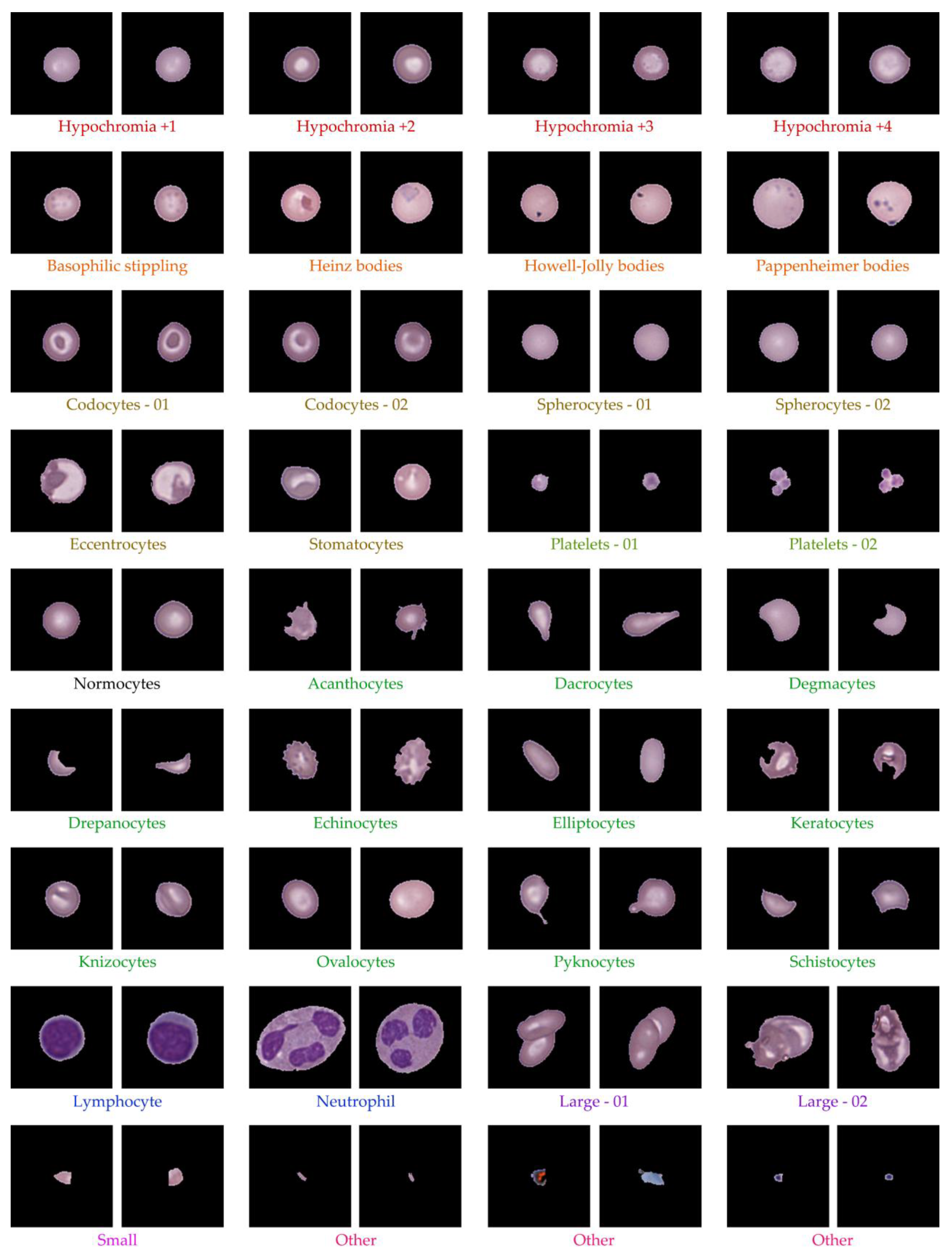
Figure 10.
Examples of RBC data augmentation using scaling (S), rotation (R), and flipping (F), demonstrating preserved morphology and increased dataset diversity.
Figure 10.
Examples of RBC data augmentation using scaling (S), rotation (R), and flipping (F), demonstrating preserved morphology and increased dataset diversity.
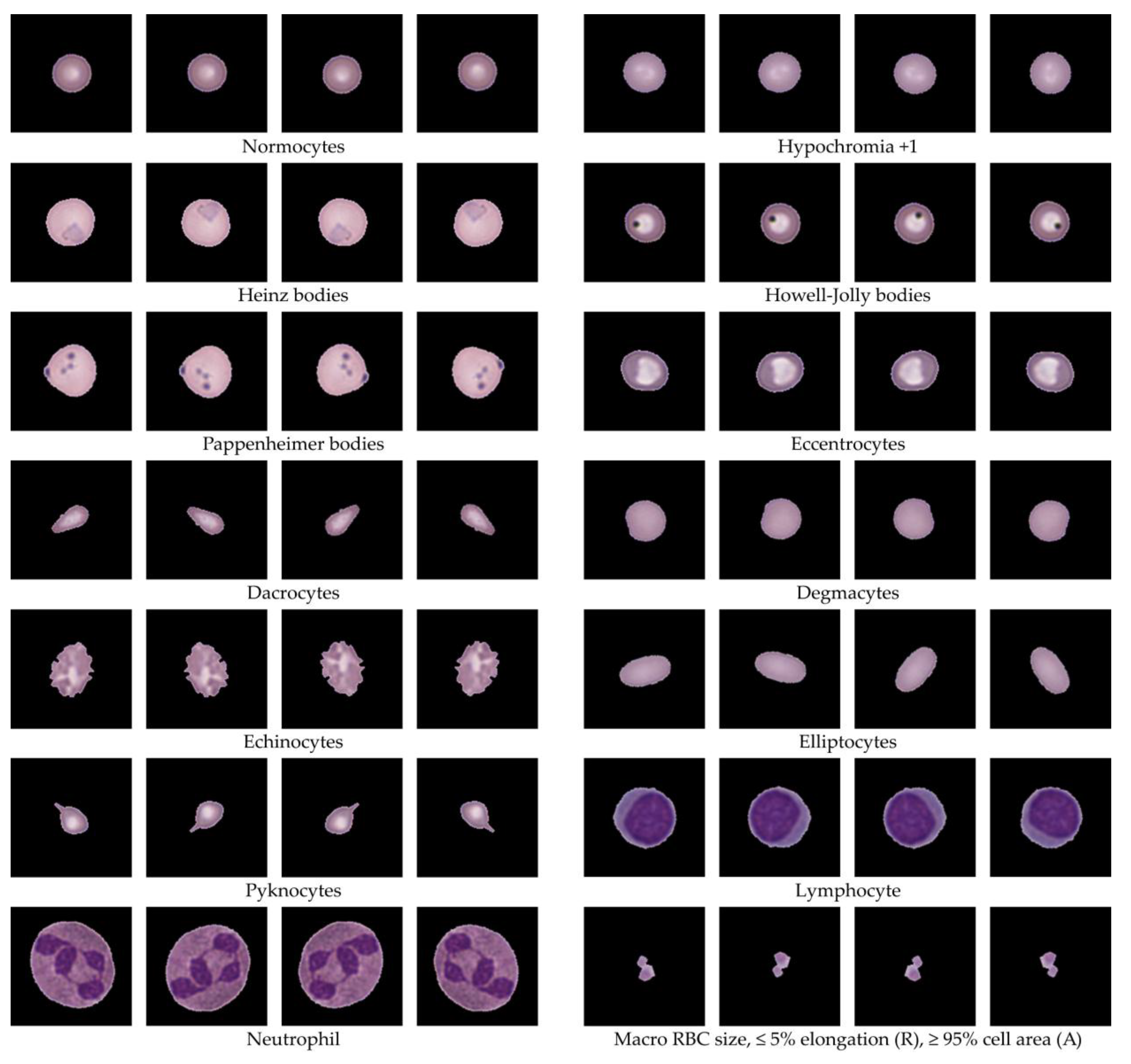
Table 1.
Cell distribution from dataset 1 across different hematological conditions.
| Sample | Single cells | Extracted cells | Overlapping | Small cells | Touching edge | Other |
|---|---|---|---|---|---|---|
| IDA | 733 | 132 | 20 | 168 | 25 | 0 |
| TT | 1,124 | 65 | 17 | 94 | 50 | 0 |
| HbH | 1,551 | 379 | 427 | 328 | 70 | 0 |
| HbE/β-thal | 5,009 | 732 | 476 | 590 | 104 | 0 |
| HbE/β-thal Sx | 930 | 445 | 211 | 853 | 63 | 0 |
| Homo HbE | 2,803 | 148 | 93 | 204 | 68 | 0 |
| Total | 12,150 | 1,901 | 1,244 | 2,237 | 380 | 0 |
Table 2.
Cell distribution from dataset 2 across different hematological conditions.
| Sample | Single cells | Extracted cells | Overlapping | Small cells | Touching edge | Other |
|---|---|---|---|---|---|---|
| IDA | 785 | 164 | 30 | 853 | 35 | 0 |
| TT | 1,874 | 239 | 381 | 298 | 59 | 0 |
| HbH | 1,167 | 270 | 362 | 232 | 68 | 0 |
| HbE/β-thal | 2,443 | 640 | 496 | 415 | 71 | 0 |
| HbE/β-thal Sx | 381 | 280 | 174 | 723 | 49 | 0 |
| Homo HbE | 3,013 | 240 | 271 | 291 | 66 | 0 |
| Total | 9,663 | 1,833 | 1,714 | 2,812 | 348 | 0 |
* The cell counts shown in these tables do not directly correlate with the type of hematological condition but depend primarily on the size of each ROI. In this study, ROIs varied in size across samples. Additionally, the counts in the Extracted cells and Overlapping cells categories represent multi-cell clusters rather than one cell per image.
Table 3.
Distribution of RBC morphological classifications in Dataset 1 after expert review.
| Class name | Morphological name | Count | Percentage |
|---|---|---|---|
| Normocytes | Normocytes * | 805 | 5.75% |
| Alteration in staining |
Hypochromia +1 * | 1698 | 12.13% |
| Hypochromia +2 * | 1059 | 7.56% | |
| Hypochromia +3 * | 240 | 1.71% | |
| Hypochromia +4 * | 47 | 0.34% | |
| Erythrocyte inclusions | Basophilic stippling | 1 | 0.01% |
| HbH inclusions | 0 | 0.00% | |
| Diffuse basophilia | 0 | 0.00% | |
| Cabot ring | 0 | 0.00% | |
| Hb H | 0 | 0.00% | |
| Hb C crystal | 0 | 0.00% | |
| Hb SC crystal | 0 | 0.00% | |
| Heinz bodies | 2 | 0.01% | |
| Howell-Jolly bodies | 47 | 0.34% | |
| Pappenheimer bodies | 16 | 0.11% | |
| Variations in Hb distribution |
Codocytes - 01 ** | 1024 | 7.31% |
| Codocytes - 02 ** | 1050 | 7.50% | |
| Eccentrocytes | 202 | 1.44% | |
| Spherocytes - 01 ** | 1718 | 12.27% | |
| Spherocytes - 02 ** | 1205 | 8.61% | |
| Stomatocytes | 173 | 1.24% | |
| Variations in RBCs shape |
Acanthocytes | 16 | 0.11% |
| Dacrocytes | 396 | 2.83% | |
| Degmacytes | 393 | 2.81% | |
| Drepanocytes | 25 | 0.18% | |
| Echinocytes | 27 | 0.19% | |
| Elliptocytes * | 136 | 0.97% | |
| Keratocytes | 7 | 0.05% | |
| Knizocytes | 525 | 3.75% | |
| Ovalocytes * | 0 | 0.00% | |
| Pyknocytes | 603 | 4.31% | |
| Schistocytes | 488 | 3.49% | |
| Leukocytes | Basophil | 1 | 0.01% |
| Eosinophil | 0 | 0.00% | |
| Lymphocyte | 21 | 0.15% | |
| Monocyte | 2 | 0.01% | |
| Neutrophil | 9 | 0.06% | |
| Platelets | Platelets - 01 ** | 312 | 2.23% |
| Platelets - 02 ** | 61 | 0.44% | |
| Others | Large - 01 ** | 766 | 5.47% |
| Large - 02 ** | 537 | 3.84% | |
| Small | 117 | 0.84% | |
| Other | 271 | 1.94% | |
| Total | 14,089 | 100.00% | |
* RBC morphology distribution in Dataset 1 after expert review. Some clusters were classified using ellipse fitting due to subtle differences in circularity or elongation, and certain morphologies were split into clear and unclear subgroups.
Disclaimer/Publisher’s Note: The statements, opinions and data contained in all publications are solely those of the individual author(s) and contributor(s) and not of MDPI and/or the editor(s). MDPI and/or the editor(s) disclaim responsibility for any injury to people or property resulting from any ideas, methods, instructions or products referred to in the content. |
© 2025 by the authors. Licensee MDPI, Basel, Switzerland. This article is an open access article distributed under the terms and conditions of the Creative Commons Attribution (CC BY) license (http://creativecommons.org/licenses/by/4.0/).
Copyright: This open access article is published under a Creative Commons CC BY 4.0 license, which permit the free download, distribution, and reuse, provided that the author and preprint are cited in any reuse.


