Submitted:
06 August 2025
Posted:
08 August 2025
You are already at the latest version
Abstract
In the process of reviewing our papers on controller design methods, we very often encounter reviewers' demands that are almost never met in most papers in this area. Our responses to reviewers with explanations do not always convince them. In this regard, several papers describing our results in this area have been rejected by reviewers, or we have been forced to make so many corrections to them that in many cases the essence of the paper is partially lost. At the same time, in each paper we have to explain anew what should be clear to a specialist in automatic control theory, otherwise he cannot be considered a specialist in this area. The most surprising thing is that we often encounter published papers that contain such gross errors or inconsistencies that one can only wonder how two or three reviewers and the editor-in-chief could accept such papers for publication. We analyze one such example of a paper that should not have been published under any circumstances. But the problem is not this article, but a large number of similar articles that also should not have been published.
Keywords:
controller
; feedback
; control error
; automatic control theory
; PID
; non-integer differentiation
; non-integer integration
; typos
; errors
; fake
1. Introduction
The problem of designing regulators for controlling a wide variety of objects has been of interest for many decades. Many publications proposing new control methods can be divided into two large classes: those that contain numerical examples confirming the effectiveness of the method, and those that do not contain such examples.
The reader has the right not to trust the second class.
In the class of publications containing numerical examples, two subclasses can also be distinguished: those in which the provided data on the mathematical model of the object is sufficient and those in which at least one parameter necessary for a complete description of the model of the object is missing.
The reader has the right not to trust the second subclass of the first class of articles.
Finally, in the first subclass of the first class, two types of articles can also be distinguished: those in which the modeling results are sufficient to assess the effect of applying these methods, and others.
In this subsection, one can also highlight articles in which the results are compared with the application of other known methods to the same numerical examples, and others.
Thus, in our logic, the most interesting articles are those that not only propose a new method or modification of a known control method, but also contain examples that have a sufficiently complete mathematical model of the object, present the results in the form of a regulator model and in the form of the obtained transient processes, and compare these results with the results of using other previously known methods.
We consider an additional highly desirable property of the presented results to be the absence of errors in obtaining and demonstrating these results.
In addition, as a desirable property of examples, we would like to see such models of objects that can be physically implemented. In particular, we consider the mathematical model in the form of a linear low-pass filter without a delay link in this model to be impossible to implement in practice, which was previously shown in our publications. Also, we, like all automation specialists, consider it impossible to implement mathematical models in the form of transfer functions in which the degree of the polynomial in the numerator is greater than the degree of the polynomial in the denominator.
We are also not interested in publications in low-ranking journals or publications that were published more than ten years ago.
Based on the principles indicated, we have made a small selection of articles in the field of designing regulators for linear and, if we come across them, also for nonlinear objects. We are interested in the efficiency of the proposed methods in comparison with well-known methods, and are also largely interested in the reliability of the information presented in these articles.
2. Materials and Methods
The materials for the research are those rare articles on automation that simultaneously contain: a) a mathematical model of controlled objects; b) a mathematical model and structure of controllers; c) graphs of transient processes obtained in the system.
The research method consists of mathematical modeling of the object and controller and numerical optimization of the controller. The research method also consists of using and, if necessary, modifying the previously proposed conditions and the objective function for optimization. The method of comparing the results consists of assessing the transient processes in the found articles taken as a standard and in our own calculations. The quality criteria for the obtained and standard systems are the duration of the transient process before entering the 2% zone of the prescribed value, the amount of overshoot, and the presence or absence of a reverse process.
3. Results
In this regard, our attention was drawn, for example, to the article [1]. It was supposed to analyze at least a dozen similar publications, but this article provided so much material that we could no longer pay sufficient attention to other similar publications within the framework of one of our articles.
The authors of the article [1] propose a new method in their understanding, which consists of using a PIDDα -controller. The essence of such a controller is that it uses four channels of a sequential controller: three of them are traditional, proportional (P), integrating (I) and differentiating (D), and the fourth contains differentiation to a fractional power of α. This method cannot be considered new, since controllers with non-integer differentiation and integration have been known for several decades, including differentiation and integration of an order greater than one.
In addition, the authors of this article do not seem to understand what the term “non-integer differentiation” means. Also, by some indications, the authors do not know how to correctly express their thoughts using mathematical notation.
This did not stop them from publishing their article in a highly respected journal [1], even though the article had to be read by at least two reviewers and the editor-in-chief of the journal.
Let’s examine this article in detail. To begin with, the authors propose a completely correct PID controller equation:
In this equation, Kp, Ki, and Kd are the coefficients of the proportional, integrating, and differentiating paths, respectively, constants that must be calculated when designing the controller. Here, the notation in the operator domain of Laplace transforms is used: is the controller transfer function, we usually use the notation ; is the task or signal of the value prescribed for the output, we usually use the notation ; is the control error; is the output signal of the object, which is also the output signal of the system; is the control signal, that is, the signal under the action of which the object must change its output signal in the desired way.
The authors of the article also consider another controller, called the PIDD2 controller. It differs by adding a channel with double differentiation and with a coefficient Kd2. The equation of such a controller is widely known, it has the form:
Next, the authors introduce the concept of FOPID, that is, Fractal-Order PID. The following equation is given for such a controller:
This is also a well-known relation, but as a rule the symbol is used to denote a non-integer degree of integration , rather than the symbol . This is important, since there is a whole line of literature that calls regulators of the form (3) regulators, but no one uses the term . The authors also make another minor typo, namely, they give the equation for non-multiple differentiation in the following form, according to the Riemann–Liouville definition:
In this case, continuity of the function on the interval [a, b] is required, despite the fact that the variable b is missing from relation (4). Here it should be pointed out that continuity of the function is required on the interval [a, x], and we are talking about a definite integral on this interval, and not just an integral. In addition, it is not clear why a new variable q is introduced if we require a non-integer integral of degree . All this is trifles, compared to the subsequent gross errors of the authors of the article [1].
It should be noted that the authors groundlessly attribute to themselves the authorship of a regulator in which non-integer differentiation and first-order differentiation are present. The equation of such a regulator is:
Here is a non-integer exponent. The authors then say that when this controller degenerates into a regular PID controller, and when it turns into a PIDD2 controller.
Of course, one can practice calculating the coefficients for such a regulator, but it is completely unacceptable to attribute the authorship of such a regulator to oneself, claiming that this regulator is proposed by this article.
The reviewers should reject the paper for claiming that the paper proposes such a controller. It is known before [2]. At least in our paper [2] we not only discussed such a controller and a more complex one, which has both integer integration paths, integer differentiation paths, and a non-integer differentiation path greater than one, as well as a non-integer integration path greater than one, but we also presented a method for modeling such a system using a system that performs only integer integration and differentiation, and also presented a method for calculating all the coefficients for this controller and demonstrated the resulting transient processes in such a system. In particular, Figure 18 in this publication shows a circuit for modeling a controller that contains six channels and can be described by the following relationship:
It is quite obvious that in the case equation (6) goes over to equation (5), up to the notation , .
In general, the well-known idea of using non-integer degrees of differentiation and integration together with the well-known idea of using differentiation and integration of a high order along with the first order makes even more complex controllers known, in particular, containing integration and differentiation of both integer order, with exponents of 1, 2, and more, and non-integer order with exponents in the intervals from 0 to 1, from 1 to 2, and so on. We do not talk about our publication [2], since in it we did not try to attribute to ourselves the authorship of such controllers, the publication [2] is devoted to the methods of implementing such a controller and studying the capabilities of such a controller using the method of numerical optimization of its coefficients.
Conclusion 1. The authors of the article [1] groundlessly attribute to themselves the authorship of a regulator of the type (5), which is a special case of the widely known regulator of the type (6).
Next, the authors of the article [1] consider four numerical examples, with the help of which they try to prove the advantage of the regulator they supposedly proposed. Unfortunately, the examples provided are not done carefully enough, and we refute all four examples. In all four examples, the authors propose to compare systems with the known regulators PID, PIDD2, FOPID, and the one they attribute to themselves and called PIDDα.
Example 1. This example proposes the design of a controller for an object whose transfer function is given by the following relationship:
Let us note right away that the attempt to optimize the PID controller for the object (7) is wrong. For such a system, it is sufficient to use a PI controller, with which one can obtain an arbitrarily high-quality transient process with an arbitrarily short duration. This follows directly from the theory. Differentiation is not required, double differentiation is not required even more so, as non-integer differentiation greater or less than one is not required. If the object had a higher-order polynomial in the denominator, or if there was a delay in the object model, this could be useful, but not in the case of the ideal transfer function (7).
The authors of the article implement some strange way of comparing the efficiency of different regulator structures. Namely: they fixed three coefficients at the following values: , , , and also in the presence of a circuit with integer double differentiation or with non-integer differentiation, the coefficient of this circuit is also fixed and it is equal to . But at the same time, for the case of the FOPID regulator, the corresponding coefficients for unknown reasons were chosen equal to , , and for the regulator supposedly proposed by them they chose .
Table 1 shows these parameters, as well as the values of the transient process indicators: the time of the first achievement of the prescribed task , the duration of the process , and the overshoot M%.
It should be noted right away that the exponent of non-integer integration differs so little from the value of first-order integer integration that it would be entirely possible to assume and not pretend that this 2% difference of non-integer integration from the integer can have any significance. It should also be taken into account that implementing non-integer integration in practice is significantly more difficult than implementing the integer, so that this option makes absolutely no sense.
Thus, the authors provide graphs with different transient processes for the specified types of regulators. We cite these graphs in Figure 1.
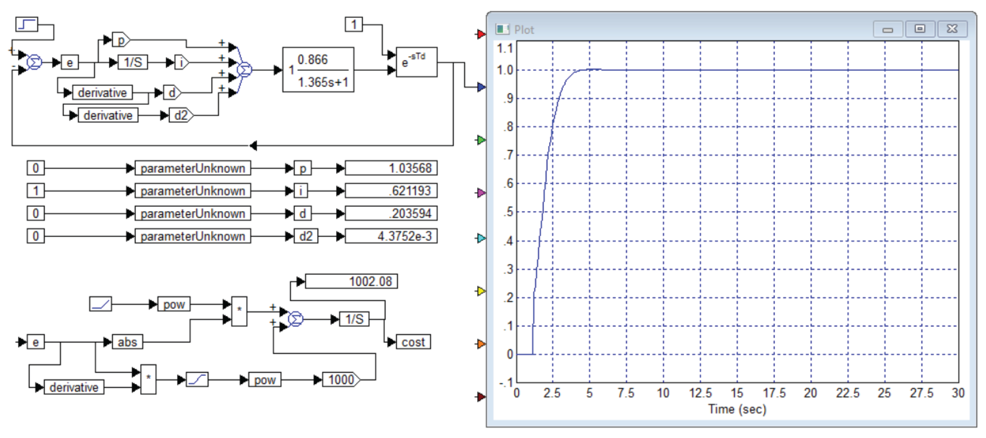
We have simulated the system and with a conventional PID controller we have obtained the transient process shown in Figure 2. In order for each reader to be able to check the reliability of the presented results, we present in Figure 3 the entire project for simulating and optimizing the controller for this object (7) from Example 1 of publication [1].
The process shown in Figure 2 is obtained with the following values of the controller coefficients: , , . Rounding the coefficients to values with an accuracy of no more than 1% does not lead to noticeable changes in the transient processes, which is verified by modeling.
As we can see, in the graphs from the article [1] all processes last from 14 seconds to 28 seconds (the values are taken from the table in the article [1]), in our graph the process ends in no more than 0.5 seconds, which is 28 times better than the best solution from the article [1]. At the same time, our process is completely free of overshoot, while in all the graphs given in the article overshoot is present, and it is from 9.6% to 22.8%, the numerical values are taken from the article [1], the graphs confirm these values.
Conclusion 2. The results proposed for comparison in the article [1] for Example 1 are not indicative, since they are very far from optimal; without any particular difficulties, much better results were obtained with a traditional PID controller.
We have indicated that for an object with a mathematical model of the form (7) there is no optimal controller. Let us demonstrate this. To do this, we will reduce the integration step to 0.01 seconds. We will obtain a transient process, the duration of which is 0.1 seconds. In this case, the controller coefficients are: , , . Rounding to 1% also does not change the type of the transient process. For persuasiveness, we provide in Figure 4 the complete project and the graph of the transient process on the oscilloscope within the framework of this project.
This system is 140 times faster than the best system obtained with the same object in the article [1]. If the integration step is further reduced, an even better system can be obtained. This is determined by the fact that the object model (7) is not detailed enough to solve the problem of designing a regulator for it. In this model, there are no factors that limit the system’s speed. Such a factor can only be pure delay or the order of the object (i.e., the order of the polynomial in the denominator) higher than the second.
Conclusion 3. The authors of the article [1] do not understand that an object of type (7) from Example 1 cannot serve as a test example for comparing the efficiency of different types of regulators, since it does not require the use of a complex regulator; a complex regulator is contraindicated for such an object. But this example is purely theoretical; in practice, such examples do not exist.
The authors then present a transient process in the resulting system when the object is exposed to interference with an amplitude of -0.2 units. The authors chose the input of the object, not the output, as the point of application. Since the object itself is also a filter for such interference, this situation is not indicative.
Figure 6 shows two variants of the transient process. The red line shows the response to two subsequent signals: first, a single step jump is fed to the system input, then interference in the form of a negative jump of the specified amplitude of -0.2 is fed to the object input through the adder. The blue line shows the response to the same signals, but under the condition that the interference is fed not to the object input, but to the output through the adder. In this case, the object no longer filters this interference. For this reason, the response to the same interference, but at a different point of application, is sharply different. Thus, the test in which the interference is fed through the adder to the object input is not indicative.
We deliberately used not the best system setup with the object from Example 1, because the best setup does not exist: whatever the calculated controller is, it is always possible to calculate another controller with which the system will be even better in all the main parameters. As we can see, even the intermediate option shown in Figure 2 and Figure 3 demonstrates much better results. In this case, the red line in Figure 6 should be compared with all the lines in Figure 5. The amplitude of the response to interference is no more than 10% of the interference in our case, the duration of the response does not exceed 15 seconds.
The article also gives a reaction to several successive step jumps. This is completely unnecessary, since the system is linear.
However, we can offer for comparison the corresponding transient processes in our system and in the systems described in the paper [1], which are shown in Figure 7.
Example 2. The second example involves designing a controller for an object whose transfer function is given by the following relationship:
Similar studies have been carried out for this object. In this case, identical coefficients for all identical channels contained in different regulators are taken without explanation. The regulators differ only in the presence of other channels. Table 2 shows these parameters, as well as the values of the transient process indicators: the time of the first achievement of the prescribed task , the duration of the process , overshoot M%.
This is extremely illogical. Comparing different regulators by efficiency in a system with the same object is simply absurd. For each structure, it is necessary to find the optimal coefficients of each regulator path.
This is not only illogical, it is simply ridiculous. It is as ridiculous as if, on the basis of the fact that a bicycle with two wheels copes well with its functions, but a car with only two wheels cannot drive, one were to claim that a car is worse than a bicycle.
Let us compare the results. The article [1] presents transient processes with all these types of regulators, the coefficients of which are given in Table 2.
Figure 8 shows the transient processes from the article [1] on the left, and the process obtained by us during optimization of the PIDD2 controller is shown on the right with a blue line. Note that, in general, our modeling confirms the type of transient process, but only qualitatively. Our result allows us to implement control with a transient process duration of , but the overshoot is equal to 3%.
The parameters of the regulator are as follows: , , , .
The simulation and optimization project with optimization results (numbers at the bottom right) is shown in Figure 9.
Conclusion 3. The results proposed for comparison in the article [1] for Example 2 are also not indicative, since they are very far from optimal; we obtained the best results with the traditional PIDD 2 controller.
Example 3. The third example involves designing a controller for an object whose transfer function is given by the following relationship:
At first glance, the transfer function takes a negative value at, so it seems logical that the coefficients of the PID controller and other controllers take negative values. But this does not work so clearly for the case of an object with positive poles of the transfer function. Recall that the poles of the transfer function are the roots of its polynomial in the denominator. The presence of positive poles is indicated by the presence of negative coefficients, and we call the poles positive those whose real part is positive. This indicates that the object itself is essentially unstable, that is, the response to a step jump at the input increases infinitely over time.
The paper [1] proposes a set of coefficients for various controllers according to Table 3. It also proposes a family of transient processes corresponding to these coefficients, which are shown in Figure 10.
Our result allows us to implement control with a transient duration of , but the overshoot is equal to 2%.
The parameters of the regulator are as follows: , , , .
The simulation and optimization project with optimization results (numbers at the bottom right) is shown in Figure 11.
We have simulated the system with all the controllers proposed in the paper, except for the controller in the last row of Table 3. All these systems turned out to be unstable. For this reason, we will allow ourselves to doubt the results presented in the paper [1] for the object from this example.
Despite our long experience of modeling in the VisSim program, we initially allowed ourselves to doubt our own results, since we assumed that this program might incorrectly model the transfer function of the form (9). For this reason, we carried out modeling using an alternative scheme, namely: we presented the transfer function as a system with three feedbacks, as shown in Figure 12. Modeling using this structure gave practically the same results, which makes us highly trust our modeling results in the VisSim program and doubt the results presented in the article [1].
We will show that this structure with three feedbacks is equivalent to the structure in Figure 11, since it is also described by the same transfer function (9). First, we write equation (9) in algebraic form.
The transfer function describes the ratio of the Laplace image of the signal at the output of the object to the Laplace image of the signal at its input. On this basis, we write the following equality.
Let us carry out several successive equivalent transformations with this equation.
This equation (17) describes the structure shown in Figure 12. If any of the coefficients is negative, a positive negative relationship is obtained.
Thus, we have no reason not to trust the simulation in the VisSim program, and, accordingly, there are good reasons to doubt the reliability of the proposed transient processes in the article [1] for Example 3. All systems, the parameters of the regulators of which are given in Table 3, turned out to be unstable. Additional reasons for our doubts are the fact that the article [1] does not provide an explanation of the exact method used to simulate the transfer function with non-integer differentiation. We cannot assume that relation (4) was used for the simulation.
Conclusion 4. The results proposed for comparison in article [1] for Example 3 seem unreliable.
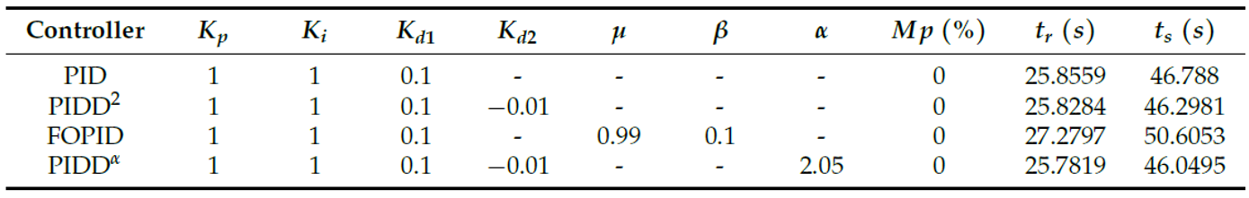
And finally, let’s consider the fourth example from the article [1].
Example 3. The third example involves designing a controller for an object whose transfer function is given by the following relationship:
Similarly, Table 4 shows the parameters of the controllers, as well as the values of the transient process indices. Also, the article [1] proposes a family of transient processes corresponding to these coefficients, which are shown in Figure 13. Our result allows us to implement control with a transient process duration of , but the overshoot is less than 0.2%. In this case, the controller parameters are as follows: ,1 , , . The project for modeling and optimization is shown in Figure 14.
Finally, it is appropriate to consider the “Experimental Study” section in article [1].
The authors report on the control of two objects having, respectively, the following transfer functions:
The authors then solve the control problems of this object using the Padé approximation. Figure 15 shows a comparison of transient processes in objects with transfer functions of the form (19) and (20), from the article [1] (dashed lines), as well as processes in models using the Padé approximation (solid lines). Figure 15a refers to model (19) and its approximation, and Figure 15b to model (20) and its approximation. It can be seen that for Figure 15a the approximation is quite close from the moment of time starting with , but at the beginning of the transient process the graphs differ significantly. In particular, the response of the Padé approximation has an inverse overshoot, i.e., the process develops in the opposite direction. This property is also largely present in Figure 15b, but the coincidence of the process graph with the exact transfer function (20) with its approximation is quite conditional, these graphs begin to coincide only starting from the value , that is, in this case only when both processes have actually ended. It is unlikely that such an approximation can be considered even exact. If in the first case for the approximation of function (19), it can be recognized that the graphs coincide for 70% of the transient process (in fractions of the amplitude at the output or in fractions of the duration of the transient process, approximately the same), then for the graphs for the approximation of function (20), the coincidence should be recognized at the level of 0%.
Next, the authors offer to the readers’ attention tables of coefficients, respectively, and indicators of transient processes, Table 5 and Table 6, as well as transient processes in the system, as Figure 16 shows. In the second case, the processes are presented incorrectly, since a significant part of the transient process is cut off; the graph in Figure 16 b shows only the positive parts of these processes, as Figure 16 shows.
The assertion that in the second case the reverse overshoot that occurs at the beginning of the transient process is cut off is confirmed by other graphs in the same article [1], for example, in the response to four successive step jumps, as shown in Figure 17. From Figure 17 it is evident that in the case for object (19) the reverse overshoot is about 20%, and for object (20) it is about 10%.
Note that reverse overshoot is the worst property of the resulting closed system. For example, if it is necessary to quickly increase the pressure in the installation, such a system begins by first reducing the pressure, and only then increasing it to the desired value. If it is necessary to urgently cool an object, such a system will begin its action with heating. If a car needs to turn left, then first it will turn right at a certain angle, and only then turn in the right direction. It is clear that in practice such a property of a closed system is in most cases extremely undesirable, and in many cases even simply unacceptable.
The authors of the article consider the presented results to be convincing evidence of the effectiveness of the management method they proposed.
This raises three natural questions.
Question 1. Why did the authors not disclose the method for implementing non-multiple differentiation?
Question 2. Why did the authors choose to use the Padé approximation if modeling the exact transfer function does not present any problems?
Question 3. For what reason do the authors of the article consider the results with reverse overshoot for both practical cases to be acceptable?
We do not have an answer to these questions, because we do not agree that non-integer differentiation or integration is easier to implement than lag. The opposite is true: lag is very easy to implement in practice and in modeling, while non-integer differentiation or integration can only be implemented approximately and by a rather cumbersome method.
The Padé approximation is also implemented in a much more cumbersome way than the exact signal delay. It can be useful only in analytical transformations of equations, but it is not exact, and therefore it can hardly be considered relevant and useful with the current development of the level of computing technology and software.
The results of control with inverse overshoot cannot be considered acceptable for any practical problems known to us, only if it is negligibly small, less than ~2%.
Also, note that transfer functions of the form (19) and (20) are too simple an example of a control object. We can offer our solution to the control problem for objects (19) and (20) using the method described earlier. The solution to each problem took less than 10 minutes.
Figure 18.
Project in the VisSim program for optimizing the PID controller for a system with an object from (19) from the publication [1] at , the transient process with this controller is shown on the right.
Figure 18.
Project in the VisSim program for optimizing the PID controller for a system with an object from (19) from the publication [1] at , the transient process with this controller is shown on the right.
For the system with object (19) our result is , , , . The admissibility of accepting the zero value is verified by modeling. In this case, the duration of the process is, overshoot . Note that with the regulator proposed in the article [1] the system provides: the duration of the process is , overshoot . In the system proposed in the article, the reverse overshoot is clearly expressed.
For the system with object (20) our result is , , , . In this case the duration of the process is, overshoot is . It has been verified by modeling that when the transient process is practically unchanged in comparison with that obtained with the values of these coefficients indicated in Figure 19.
With the regulator proposed in the article [1] the system provides: process duration , overshoot . In the system proposed in the article the reverse overshoot is clearly expressed.
4. Future Research
Readers may be surprised that we have reviewed only one paper and criticized it in such detail. The reason is that this paper at first glance seemed to us to be one of the most consistent and outwardly convincing papers compared to other papers we have reviewed in the same field.
For example, consider the paper [4]. For some inexplicable reason, the authors consider a structure with non-unit feedback and a filter at the input between the input of the reference signal and the subtractor to be a “universal feedback system” and base all their research on this misconception. This structure is shown in Figure 20. In this case, the disturbance is fed to the input of the object. Such a structure promotes self-deception. Those who obtain results that seem satisfactory to them, in fact, design a system that is far from satisfactory. Figure 21 shows how the control system should be built. In the next article, we will analyze this and other errors in the publication [4] in detail.
The article [5] is also attractive in that it contains models of objects for which control is calculated. Only the examples of models selected are such that do not allow the results of the research to be taken seriously, since they also contain excessively simple and insufficient models. These are first- and second-order filters without delay of the following type:
These examples are, firstly, obviously fictitious, secondly, they do not correspond to any real object in their form, since there is no delay in them, thirdly, the too small order of the polynomial in the denominator makes the problem of controlling such objects trivial. The article [4] contains a lot of other information, which can be divided in detail into reliable and unreliable. We will deal with this in future publications, if we find time for this. The article [7] solves an equally incorrect problem of controlling an object specified by a second-order transfer function, and at the same time hopelessly outdated tabular design methods are used, such as the Ziegler–Nichols and Cohen–Coon methods. At the same time, the use of a controller with non-integer differentiation and integration is declared. Obviously, the authors have not fully understood the problems of controlling objects, do not understand the purposes of non-integer integration and non-integer differentiation at all, and the transient processes they present also raise many questions. We can also return to this article in our future articles.
Article [8] also contains a model of the object and the obtained transient processes. In this article, four models of the object have the form of a first- and second-order filter (two models) and a fourth-order filter, in all cases there is also a delay link. Such models are sufficiently correct for solving problems of controlling these objects. This article does not contain obvious errors that can be detected during a superficial examination, so it deserves the same careful reading as article [1]. We read such articles not with the aim of refuting them, but with the aim of finding those useful results that, as we hope, are contained in them. In addition, it is not our fault that article [1] disappointed us so much; this is entirely the merit of the authors of this article.
In this article, we cannot analyze all the articles with gross errors in such detail, as we did with article [1], since even in a journal that does not set limits on the length of an article, any article must be finished.
5. Discussion
The article [1] considers four theoretical examples and two examples from real practical problems, a total of six objects. In example 3, we see incorrect modeling and an erroneous result. In example 2, we see an incorrect model that cannot describe any real object. In all cases, we obtained controllers with which the systems have the best parameters in terms of combining high speed and low overshoot, and almost everywhere these results are better in both of these parameters, and only in some cases are better in one of the parameters and comparable in the second parameter.
On this basis, we can state that the results described in the article [1] do not present any advantages over the results that can be obtained with the known (and previously described by us) methods of designing regulators and, accordingly, automatic control systems. In addition, it is important to note that this article [1] does not disclose the method of using non-integer differentiation or integration. If this method is implemented in the same way as in the article [2], then non-integer differentiation significantly complicates the mathematical model and implementation of the regulator. Alternative methods are not presented.
In the abstract, we also pointed out that reviewers sometimes unreasonably demand some clarifications or additions that should not be demanded with the persistence that reviewers often show.
The first frequently encountered requirement is that the authors of the article take examples from life, from real problems, to demonstrate the effectiveness of the method.
This requirement is not justified, and besides, this requirement is very often not met at all in many already published articles. It would be desirable in this case to approach the task of reviewing by precedent. Since very many articles are published with demonstrations of the method on hypothetical examples, and these articles are not rejected, then, in any case, these same journals or journals of the same level should remove this requirement from other authors and from other articles.
The second requirement, which is no less common, is that authors explain in detail the methods they used, even if these methods are widely known from the literature, and, in addition, knowledge of these methods is not required to solve the problems solved in the articles.
For example, the reviewer insists on a detailed explanation of the numerical optimization method used.
The point is that optimization methods themselves exist in great abundance, they have specific names, they are described in many articles, as well as in monographs and even in textbooks. For example, there are optimization methods such as the Powell method, the Hook-Jeeves method, the Polak-Ribiere method, the Fletcher-Reeves method, the Monte Carlo method, the Gauss method, and so on.
It is not difficult to find a description of the method, algorithms for its implementation, and numerous examples of how these methods work. These methods are even described in Wikipedia. In addition, if the method is a built-in method in some widely available software, then the user does not even need to know how exactly this method works in order to use it.
After all, many TV viewers do not know how a TV is built, which does not prevent them from using it. Not all computer users know how it is built, which does not prevent them from using it. Many do not know how a washing machine or dishwasher works, some do not even know how a regular kettle or toaster works. But this does not prevent them from using these items.
We might not know how optimization methods work. But we can give readers a method for applying this method, which consists of a complete set of tools: a cost function, a test signal, optimization conditions, a method for selecting the coefficients and parameters of all these functions, as well as a method for evaluating the result and a method for improving it if it does not satisfy the designer. It is also important to know whether this result can be further improved, or whether it is the best of all acceptable results and further improvement is impossible. It is also important to know which method can be used if the methods used do not give the desired result.
For example, if the use of a PID controller does not give the desired result, then it is useful for the user to know the classification of complex controllers, as well as a list of possible advantages and disadvantages of these controller options. In one case, it is advisable to add an extra double differentiation channel, in others, it is better to add a double integration channel, in other cases, it is advisable to create an additional control loop, external to the existing one. And so on. These questions take up a lot of space in the article. If we also explain how exactly the numerical optimization methods work, then the article will become too long. And what is more important, increasing the volume of the article will not make it more informative, because the author will be forced to present what is already widely known. In addition, the description of the optimization method is not the result of the authors of such an article. That is, the author is forced to explain in detail what he did not do, and sometimes even give comments on those questions that he has no idea about.
Another unreasonable requirement of reviewers is the requirement to explain observed facts. A previously unknown fact is in itself a fairly new result. If the author claims that one of the three optimization methods is more often successful, then what is the point of demanding that he explain it? Each reader can put forward his own version, but the truth may be different. The author, who is forced to respond to the reviewer’s comments, can, of course, suggest some explanation, but he may also be wrong. The reviewer in this case may be satisfied, but the article will not be any better.
As an additional remark to our assertion that examples of real objects are not obligatory, we point out that we have very good grounds for considering examples (19) and (20) not to be examples of real objects. It is enough to pay attention to the numerical values of the parameters and to the order of the objects.
In both cases, the delay value is expressed as an integer in seconds. Can such an exact coincidence exist in nature? This is despite the fact that the transmission coefficients and the first-degree coefficient in the polynomial in the denominator are given as very precise numbers, three or even four significant digits! Probably, the delay of a real object is not expressed as an integer. In addition, these objects cannot be described by a first-order model. There are several elements in the setup. Each element has its own speed. This will give a higher-order polynomial. So we can point out that authors who claim to use real models do not always use reliable models of real objects. If they simplify and round off these models, then the value of such models does not exceed the value of fictitious numerical examples.
We have previously published a preprint criticizing incorrect articles on designing controllers for objects [3]. In this preprint, we examined in more detail the reasons why models of a control object of type (7) cannot be considered sufficiently correct or detailed enough to be used to design a controller for such objects (Appendix A). There, we also pointed out errors in some articles, which we reported to the authors. For one of the articles, we received a response from the authors, in which they acknowledged that their article contained the errors or typos we had indicated, and they also acknowledged that some of the transient process graphs presented were fake.
We have to admit that at present in the field of designing regulators for various control objects a very large percentage of articles have one of the following shortcomings.
The first drawback is that reliable information is not provided in the required complete combination: information about the mathematical model of the control object, information about the mathematical model of the obtained regulator, and reliable information about the properties of the obtained system in the form of transient processes. If there are only no transient processes, then readers can calculate them, but this does not apply to all readers, so this information is very necessary. If there is no information about the model of the object or the model of the regulator, then such an article is fatally incomplete.
The second drawback is the discrepancy between one of these three types of information. Most often, the presented processes are not obtained correctly enough, that is, the modeling can show a discrepancy between the graphs that are shown and those that should take place in reality.
A third drawback may be that the results offered are far from being the best in comparison with those that could be obtained in the same or simpler way. In this case, something that is not a great achievement is declared.
The fourth drawback may be that the method of implementing the proposed regulator or the method of its design is not fully disclosed.
In the article [1] we have analyzed, we see the second shortcoming for Example 3, as well as the third and fourth shortcomings for all six examples considered. In addition, the article has an individual shortcoming, which is that the authors baselessly compare different types of regulators, assigning identical transmission coefficients to similar channels. There is also a significant shortcoming, which is that the coefficients assigned to these regulators, as shown in Table 1 - Table 6, are given without derivation, the chosen values are not justified in any way. In the case of Table 1, this is apparently a completely arbitrary choice, since it is difficult to assume that the calculation resulted in values equal to 1 or 2. This should have been indicated so that the reader would not have to guess (and the fact that this was not said is another shortcoming of this article). There are good grounds to assume that the values of the coefficients given in Table 5 and Table 6 were chosen at random, but the order of magnitude was determined empirically. In this way, coefficients with values of 1, 0.5, 0.1 and 0.01 can be obtained. However, the coefficients in Table 2, Table 3 and Table 4 are clearly not random. Most likely, they were chosen by a rough empirical method, since a coefficient equal to 8 does not look like a random value, and coefficients equal to 159 or 139 do not look like random.
The lack of indication of the method for calculating these coefficients is also a shortcoming of the article.
Another shortcoming of this article is that, having obtained values for the coefficients of the PIDD 2 controller with small negative values for objects of the form (19) and (20), the authors of the article did not even try to model systems with zero values of these coefficients. The small value itself makes one doubt the necessity of such a channel; the negative value of the coefficient of the path with differentiation of the first or second order itself makes one doubt the validity of this result, and the combination of these two features directly indicates the need to pay attention to this result and investigate whether these paths with such strange coefficients are really necessary, because this is a small positive feedback, which should amplify high-frequency interference in the path. The authors obviously insist on the significance of these coefficients, since they cited them as part of the result they obtained.
Figure 23a shows a comparison of the system with our controller (blue line) with the PIDD2 controller proposed in the article [1] for the object (20). It is evident that in our case the response speed is much higher. In addition, one can notice a small section of monotonicity violation at the moment of about . We enlarged this section in Figure 23b (blue line, marked with the number 1) and compared it with the graph obtained with a zero value of the coefficient of the double differentiation path (black line, marked with the number 2). No other differences in the graphs with these two compared controllers were revealed. Thus, the coefficient is clearly unnecessary, it is better to put and not to use this path at all in this case. This will give a better result and a simpler controller. It is a pity that the authors of the article [1] neglected this check and published this unverified result.
If an article has the drawback we named first, the article is of no interest to readers, the results presented cannot be verified. The list of articles with this drawback would be too long for us to list it, this is a very common situation.
6. Conclusions
We do not deny the usefulness of the process of peer reviewing scientific articles. Our personal experience confirms that reviewers quite often rightly point out the shortcomings of an article; implementing the reviewers’ suggestions or correcting the shortcomings they have found greatly improves the article. Reviewers can notice insufficient logic in presentation, violation of the sequence of reasoning, omissions of premises obvious to the authors but not obvious to the readers better than the authors themselves, which interferes with the perception of logic and evidence. Also, reviewers are often better than the authors themselves at noticing repetitions in presentation, excessive detail in explaining fairly clear theses or insufficient detail in explaining new theses or in drawing conclusions. All this happens very often, so the work of reviewers sometimes leads to such a significant contribution to improving the article that it would be appropriate to include them among the co-authors of the article, but this is excluded according to the generally accepted rule, and this is correct. No matter how attentive and competent the reviewer may be, he is still not a co-author. And the authors should be given the right to accept or reject the reviewers’ comments, because they are the authors, this is their scientific work, the result of their research and creativity, they cannot be forced to accept the opinion of a person who, even with all his competence and authority, still did not carry out the research that underlies any scientific article.
In this sense, preprints are of great value because they allow authors to publish their paper in its original form, without the influence of the opinions of reviewers, whether correct or incorrect. Science cannot advance without errors. Authors’ errors are their right. Reviewers’ errors are their inalienable right. Journals appoint two or more reviewers to have different views that will exclude the dominant opinion of the reviewer, especially when it is not perfect.
Perhaps science would develop more effectively if all articles that authors wished to publish were published, but their value would not be determined by the journal in which they were published, or by how many readers these articles had, or even by how many times these articles were cited. After all, in our case, we cite an article [1] not at all in order to praise it and call it a valuable contribution to science, but quite the opposite, in order to point out errors in it and in the hope that in the future authors will make fewer such errors, and readers will not accept these erroneous information as true. Criticism of published articles is no less a contribution to science than the articles themselves. And if the articles are wrong, and the criticism is fair, then the critical article is more important than the article it criticizes.
Reviewers typically ask a standard question: “What contribution does your paper make to science?”
In this case, the answer to this question is extremely easy. Take the declared contribution to science of article [1] with the opposite sign. That is, the statements of this article are erroneous, so the declared contribution is not positive, but negative. And the contribution of our article consists in canceling the contribution of article [1].
We have no subjective reasons to criticize the article [1], the so-called “conflict of interest” does not take place. We are not acquainted with the authors of the article and wish them every success and prosperity. But science should be protected from erroneous statements, so we hope to restore the truth.
We should also inform you that we do not have a habit of searching for articles with errors in order to criticize them. On the contrary, we search for scientific articles that propose new methods for solving problems in the field of our research. In particular, we actively search for articles that contain mathematical models of objects, models of regulators and results. Having found such articles, we check the correctness of the results presented. Having found errors, we mark them.
We strive to have as few errors in scientific articles as possible. We do not exclude that there may be errors in our articles as well.
We will quote Donald Foster, an English linguist (he was born in 1950): “He who is unable to rejoice at discovering his own error does not deserve the title of scientist.”
Therefore, we can hope that our article will not upset the authors of the article [1], but will please them, because, firstly, their article is read, secondly, their article is read very carefully, thirdly, they received information about errors, which will allow them to correct them, fourthly, they can receive in this article many useful recommendations on how to avoid similar errors in the future.
The author intends to submit this article to the scientific journal Algorithms, since his article is directly related to another article published in this journal. However, if the journal rejects this article, it will still be published as a preprint.
The author could have provided an extensive bibliography to add credibility to the Introduction section, but he considers this unnecessary.
This work was supported by a grant from Ministry of Education and Science of Russia on the topic “Development of scientific methods for precision optical measurements of seismic, acoustic and optical fields and methods for constructing atmospheric ultraviolet optical communication with luminescent antennas for monitoring objects with natural and anthropogenic hazards,” registration number 121033100068-7. The work was carried out with the support of the Ministry of Education and Science of Russia (within the framework of state assignment No. 075-00682-24) and using data obtained at the unique scientific installation “Seismo -infrasound complex for monitoring the Arctic permafrost zone and a complex for continuous seismic monitoring of the Russian Federation and adjacent territories of the world.”
References
- Fawwaz, M. A.; Bingi, K.; Ibrahim, R.; Devan, P. A. M.; Prusty, B. R. Design of PIDD α Controller for Robust Performance of Process Plants. Algorithms 2023, 16, 437. [Google Scholar] [CrossRef]
- Zhmud, V.; Dimitrov, L. Using the Fractional Differential Equation for the Control of Objects with Delay. Symmetry 2022, 14, 635. [Google Scholar] [CrossRef]
- V. Zhmud and L. Dimitrov. Control of Linear Multichannel Objects with Numerical Optimization. Preprint No. 202507.0554. Posted Date: 7 July 2025. [CrossRef]
- Kos, T.; Huba, M.; Vrančić, D. Parametric and Nonparametric PID Controller Tuning Method for Integrating Processes Based on Magnitude Optimum. Appl. Sci. 2020, 10, 6012. [Google Scholar] [CrossRef]
- Ding, Y.; Ren, X.; Zhang, X.; Liu, X.; Wang, X. Multi-Phase Focused PID Adaptive Tuning with Reinforcement Learning. Electronics 2023, 12, 3925. [Google Scholar] [CrossRef]
- Batiha, I.M.; Ababneh, O.Y.; Al-Nana, A.A.; Alshanti, W.G.; Alshorm, S.; Momani, S. A Numerical Implementation of Fractional-Order PID Controllers for Autonomous Vehicles. Axioms 2023, 12, 306. [Google Scholar] [CrossRef]
- Batiha, I.M.; Ababneh, O.Y.; Al-Nana, A.A.; Alshanti, W.G.; Alshorm, S.; Momani, S. A Numerical Implementation of Fractional-Order PID Controllers for Autonomous Vehicles. Axioms 2023, 12, 306. [Google Scholar] [CrossRef]
- Kula, K.S. Tuning a PI/PID Controller with Direct Synthesis to Obtain a Non-Oscillatory Response of Time-Delayed Systems. Appl. Sci. 2024, 14, 5468. [Google Scholar] [CrossRef]
Figure 1.
Graphs of transient processes with different controllers for Example 1 from the publication [1].
Figure 1.
Graphs of transient processes with different controllers for Example 1 from the publication [1].
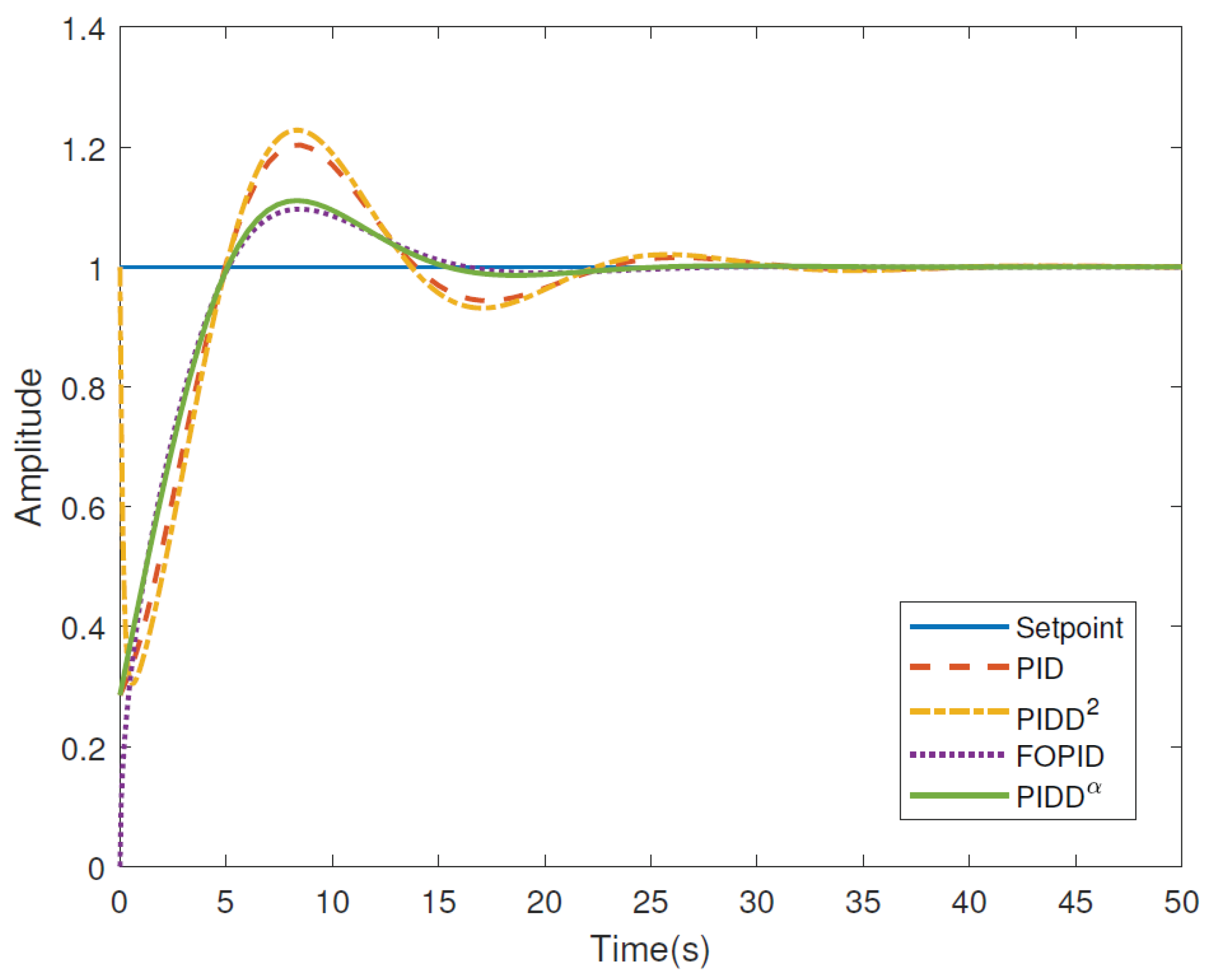
Figure 2.
Transient process in the system with the object from Example 1 from publication [1] using a PID controller optimized in the VisSim program.
Figure 2.
Transient process in the system with the object from Example 1 from publication [1] using a PID controller optimized in the VisSim program.
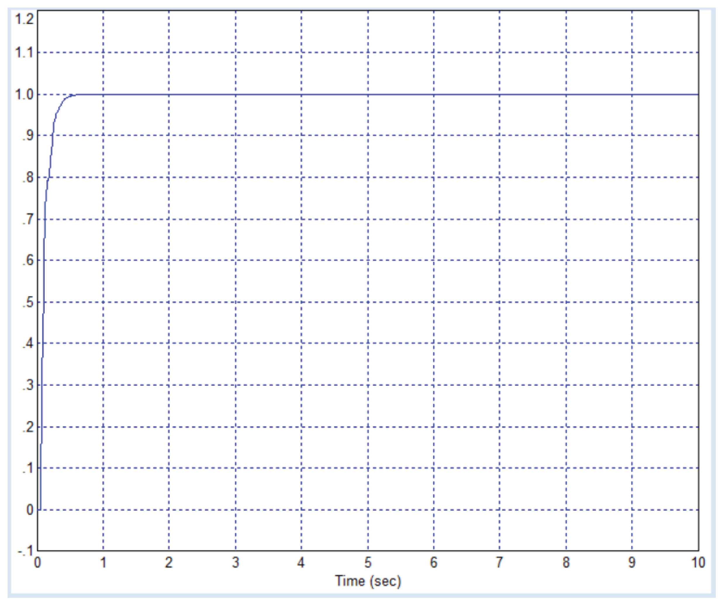
Figure 3.
Project in the VisSim program for optimizing the PID controller for a system with an object from Example 1 from the publication [1] with a discrete time step , the transient process with this controller is shown in Figure 2, the obtained values of the PID controller coefficients are shown in the displays in the center of the figure on the right.
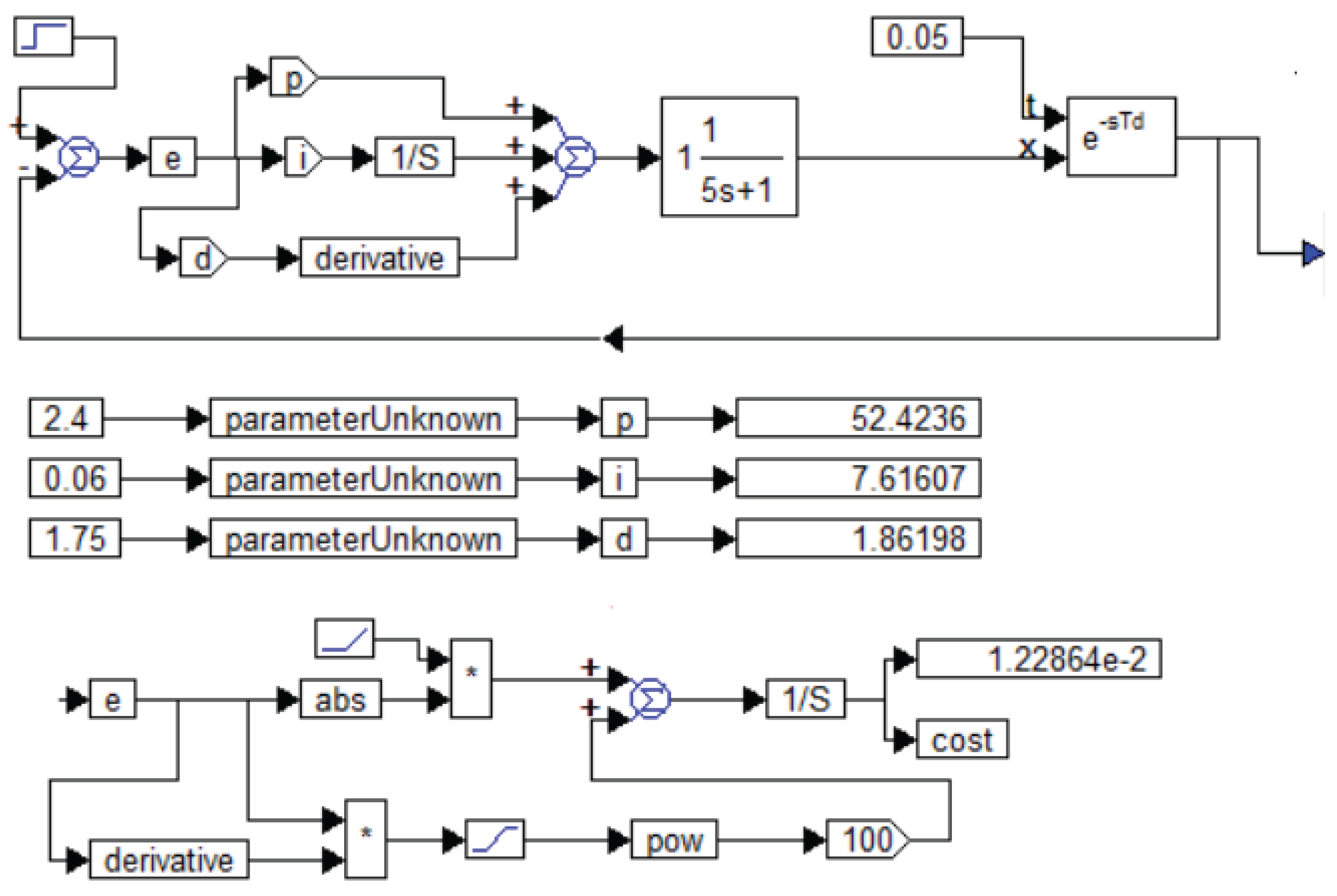
Figure 4.
Project in the VisSim program for optimizing the PID controller for a system with an object from Example 1 from the publication [1] at , the transient process with this controller is shown on the right.
Figure 4.
Project in the VisSim program for optimizing the PID controller for a system with an object from Example 1 from the publication [1] at , the transient process with this controller is shown on the right.
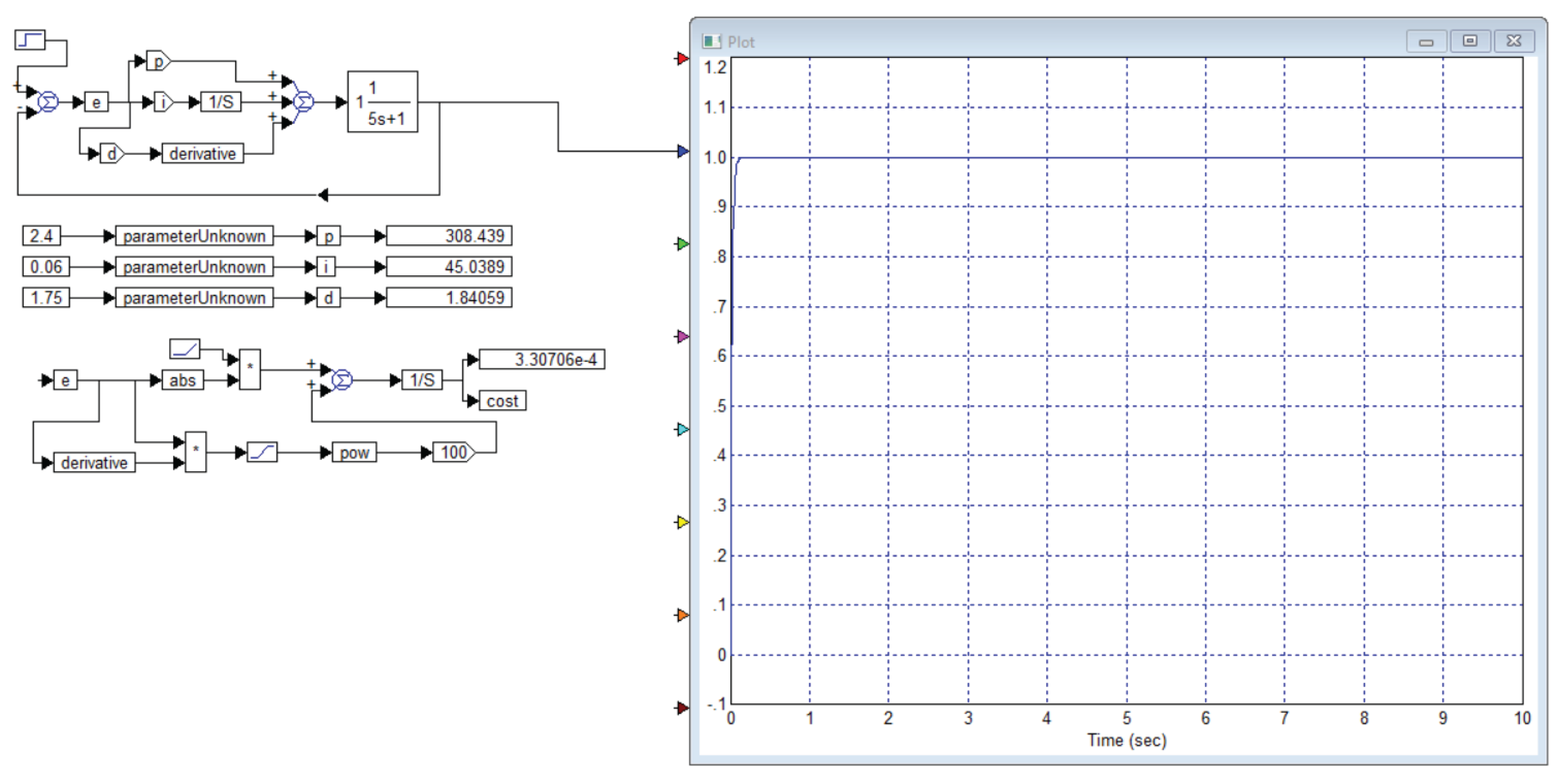
Figure 5.
Transient processes in the system with the object from Example 1 from the article [1].
Figure 5.
Transient processes in the system with the object from Example 1 from the article [1].
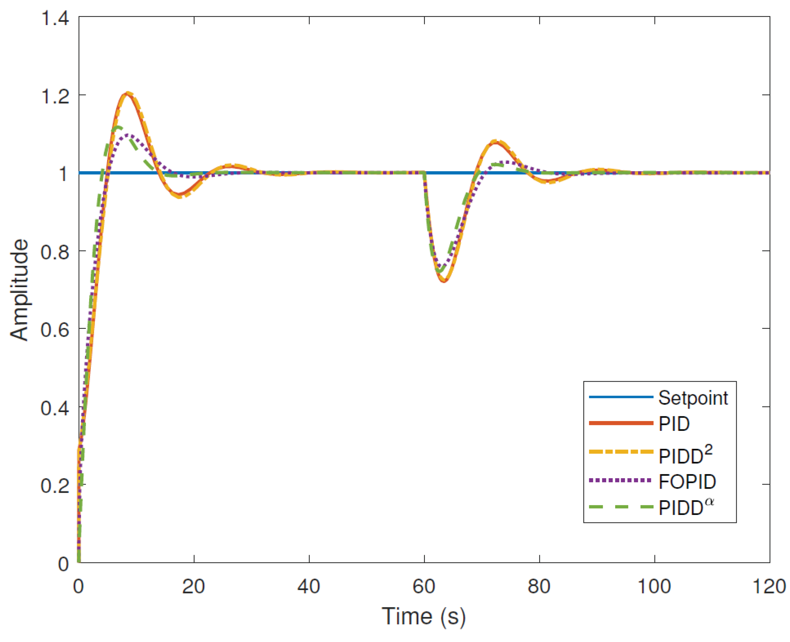
Figure 6.
Two variants of the transient process in the system, according to Figure 3, when a step signal is applied to the input and when interference with an amplitude of -0.2 units is applied: blue line – interference is applied to the output of the object, red line – interference is applied to the input of the object.
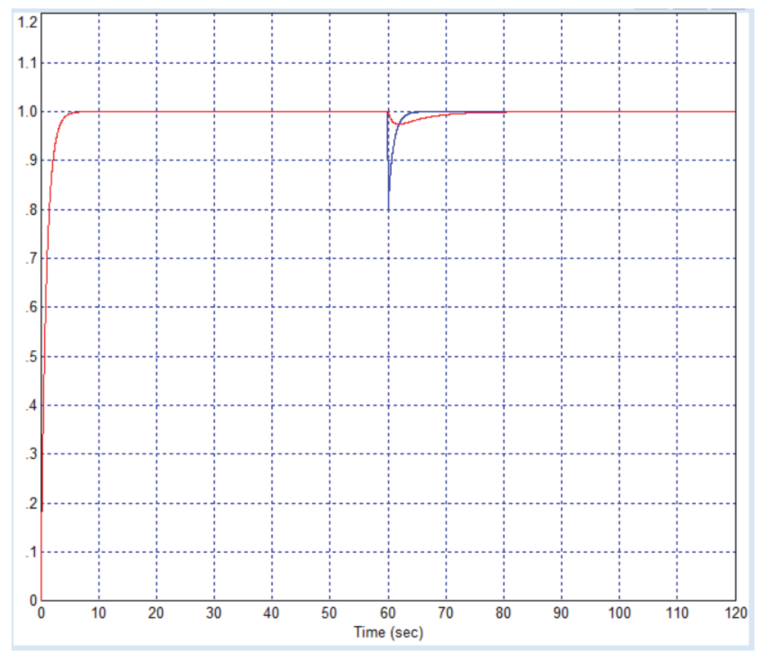
Figure 7.
Comparison of transient processes for four jumps of the task, given in the article [1] – Figure 7a, and obtained in our system for exactly the same jumps – Figure 7b, the graphs are given in the same scales.
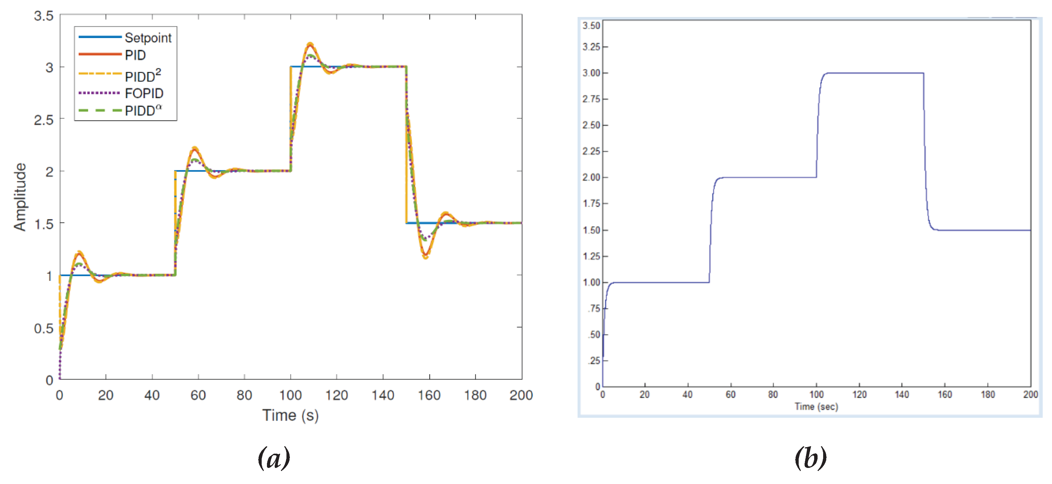
Figure 8.
Comparison of transient processes in the system with the object from Example 2, given in the article [1] – Figure 8a, and obtained in our system with exactly the same jumps – Figure 8b, the graphs are given in the same scales.
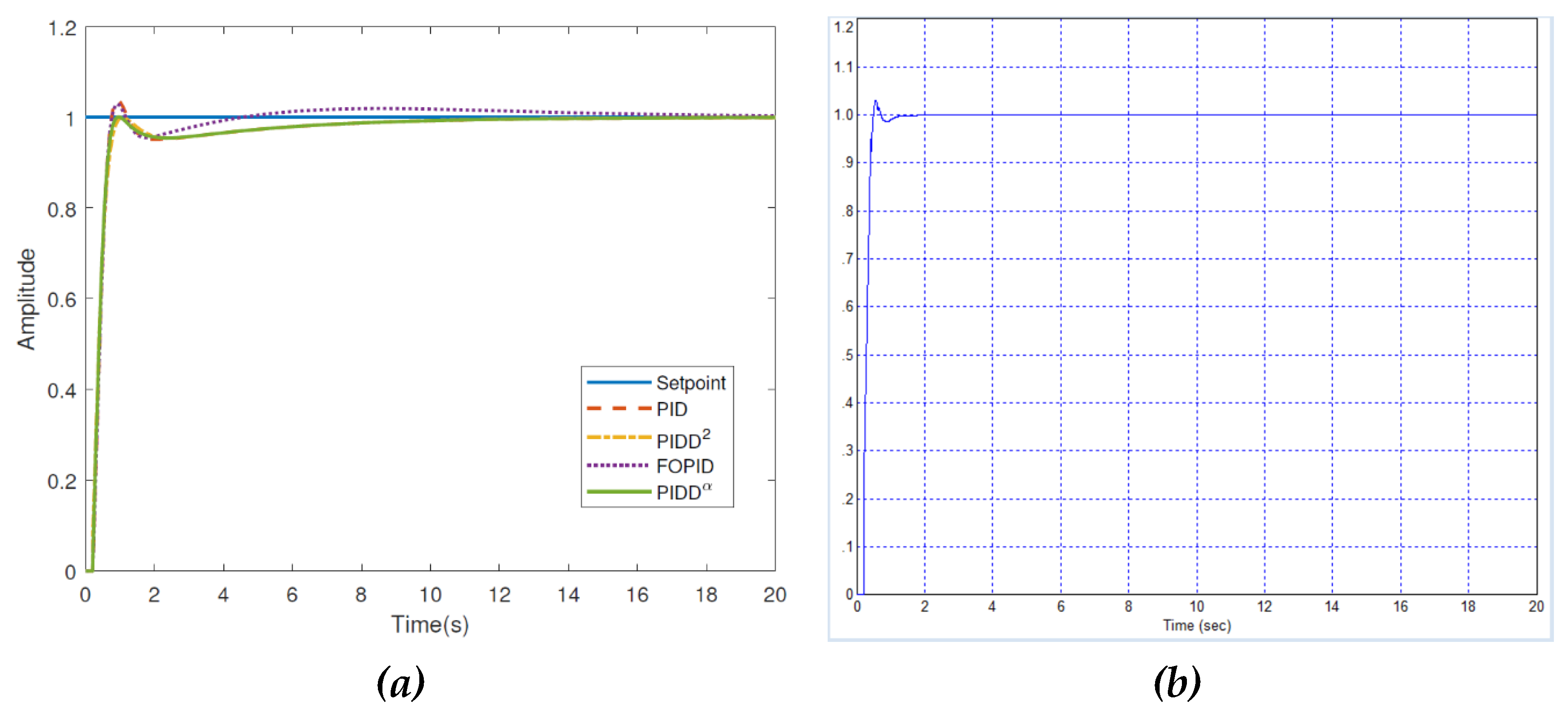
Figure 9.
Project in the VisSim program for optimizing the PID controller for a system with an object from Example 2 from the publication [1] at , the transient process with this controller is shown in Figure 8, b.
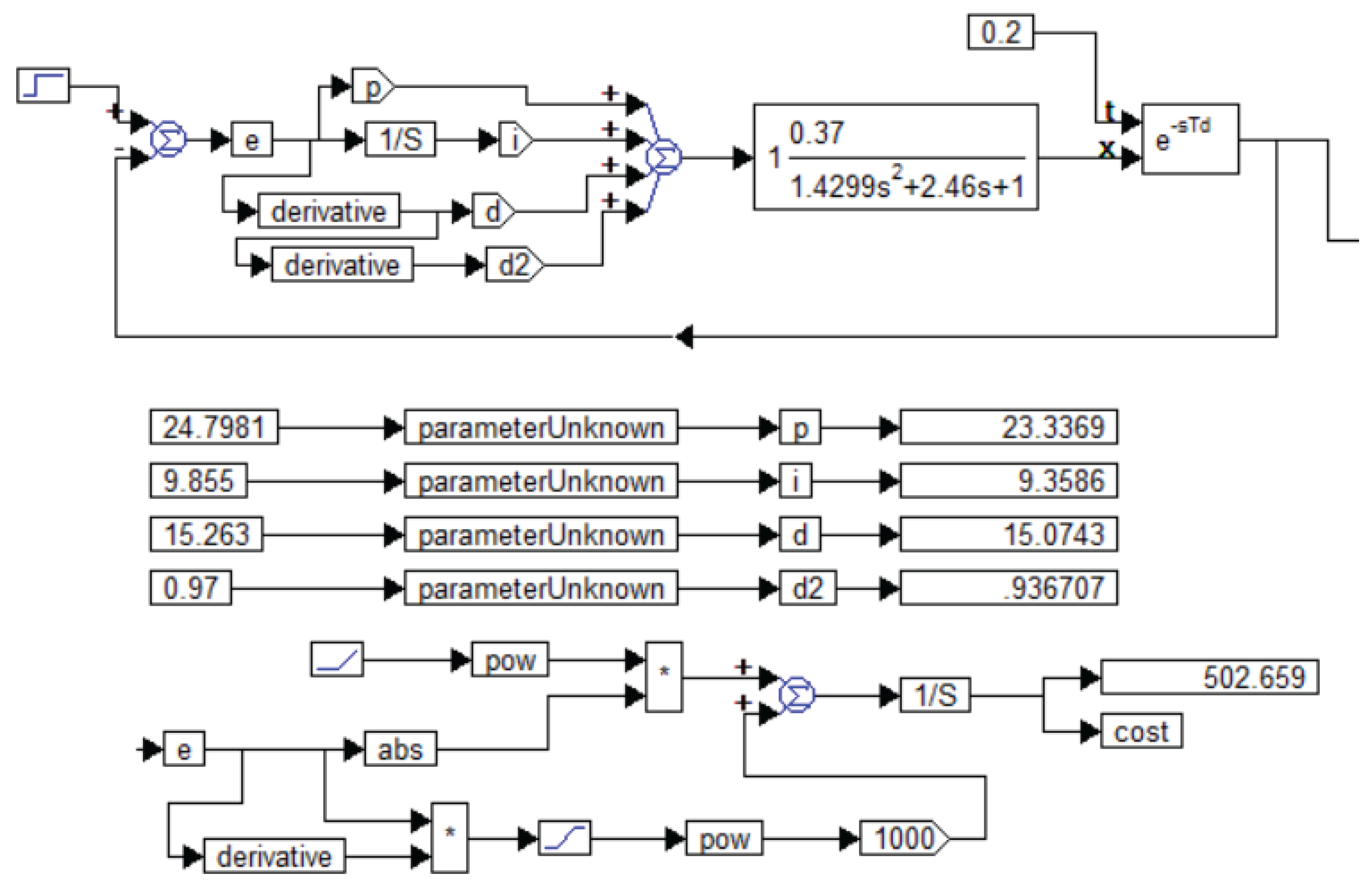
Figure 10.
Comparison of transient processes in the system with the object from Example 3, given in the article [1] – Figure 10a, and obtained in our system with exactly the same jumps – Figure 10b, the graphs are given in the same scales.
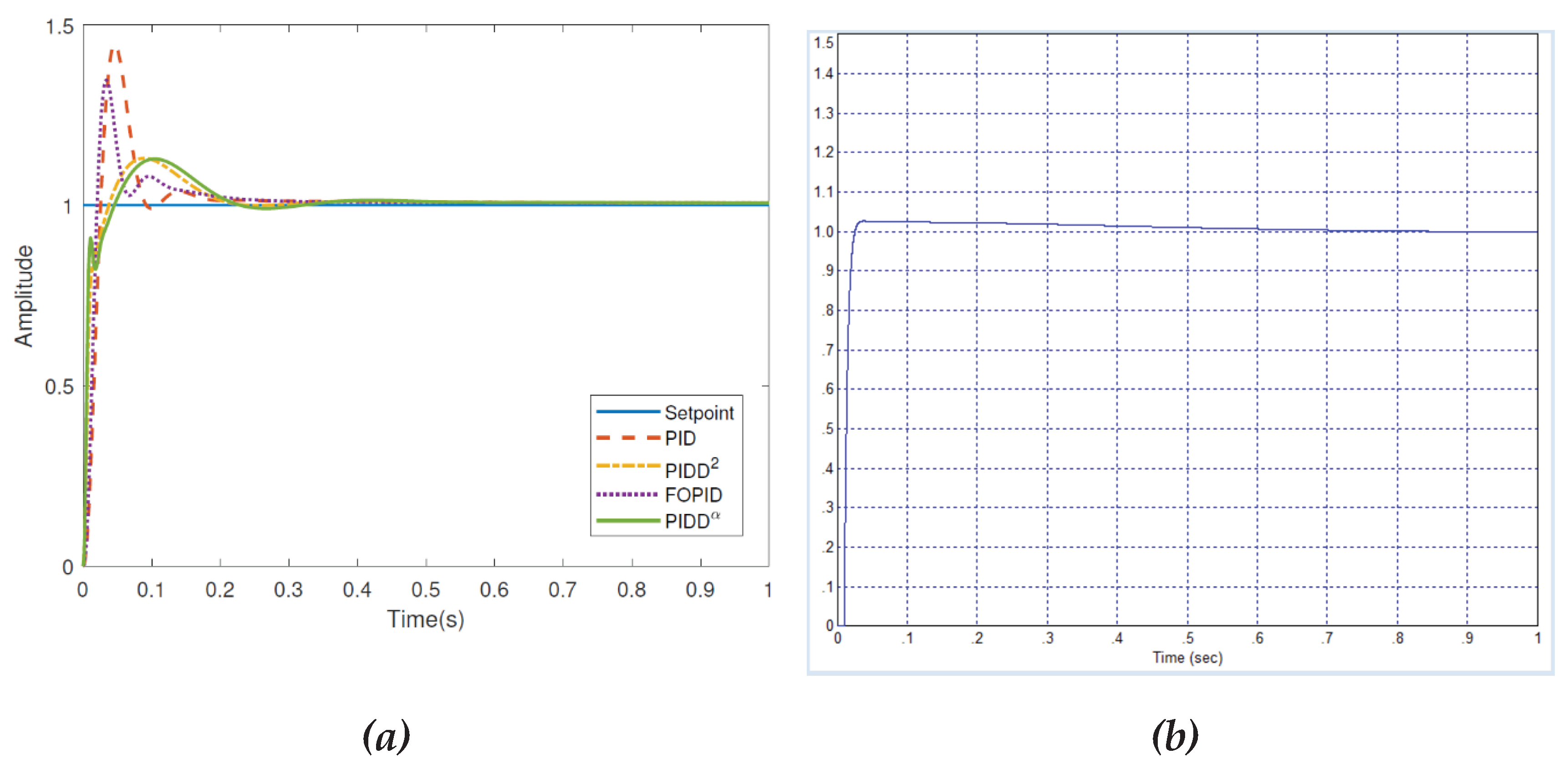
Figure 11.
Project in the VisSim program for optimizing the PID controller for a system with an object from Example 3 from the publication [1] at , the transient process with this controller is shown in Figure 10, b.
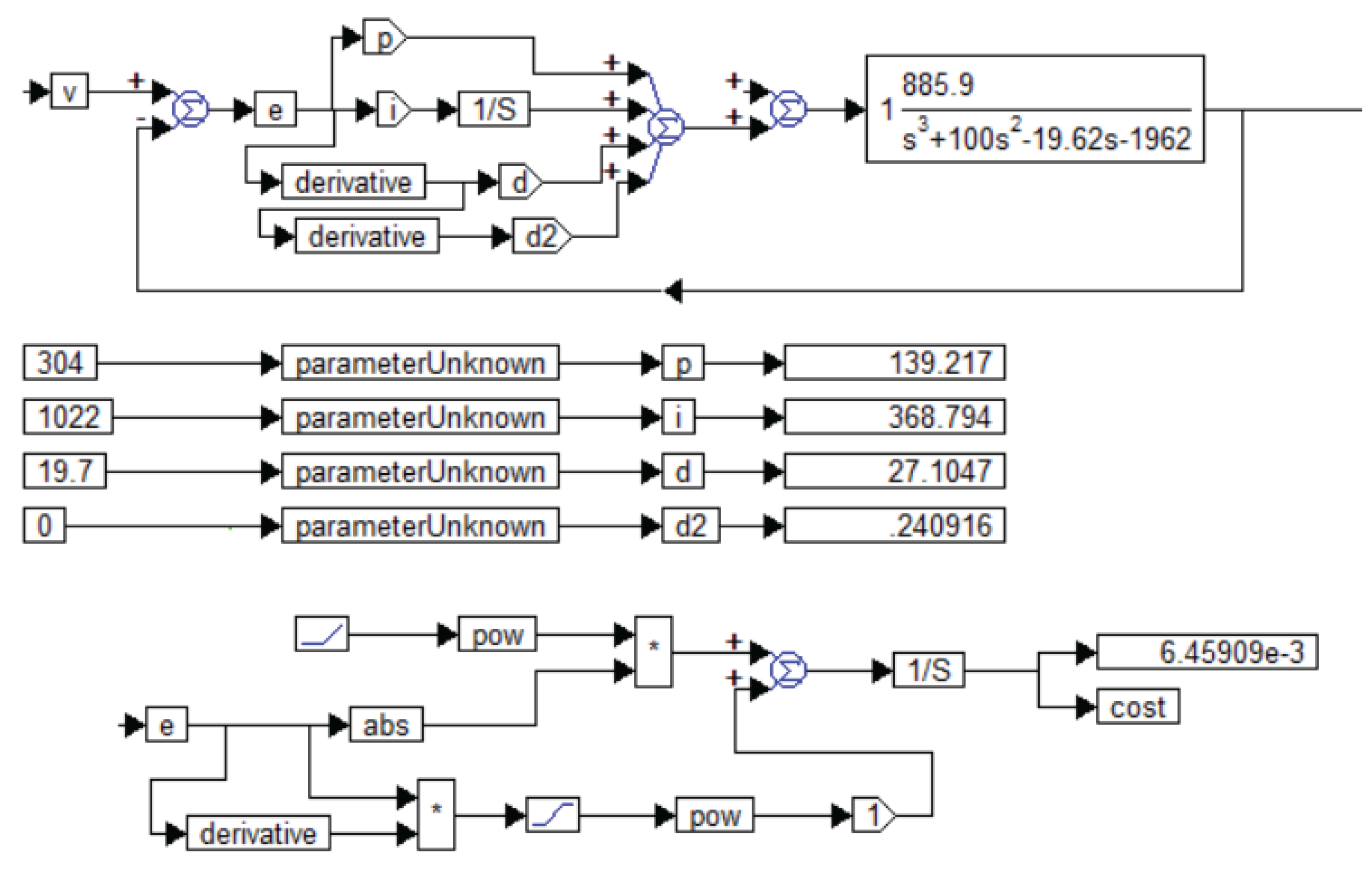
Figure 12.
The VisSim program project for modeling the object from Example 3 from publication [1] and the PID controller, this structure was also used for optimization with the same result as shown in Figure 10, b.
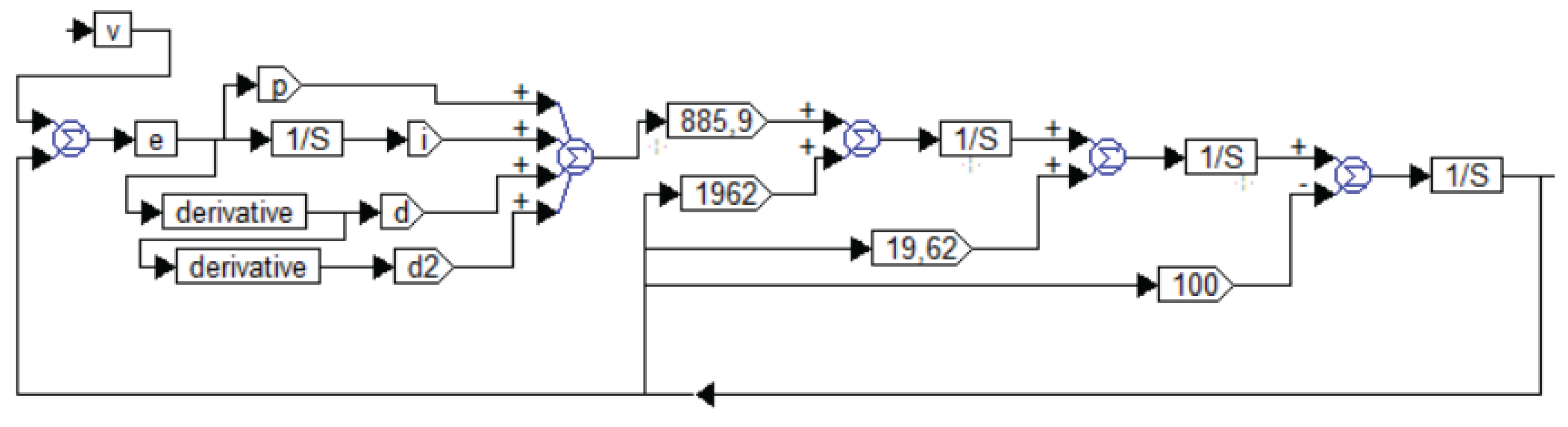
Figure 13.
Comparison of transient processes in the system with the object from Example 4, given in the article [1] – Figure 13 a, and obtained in our system with exactly the same jumps – Figure 13 b, the graphs are given in the same scales.
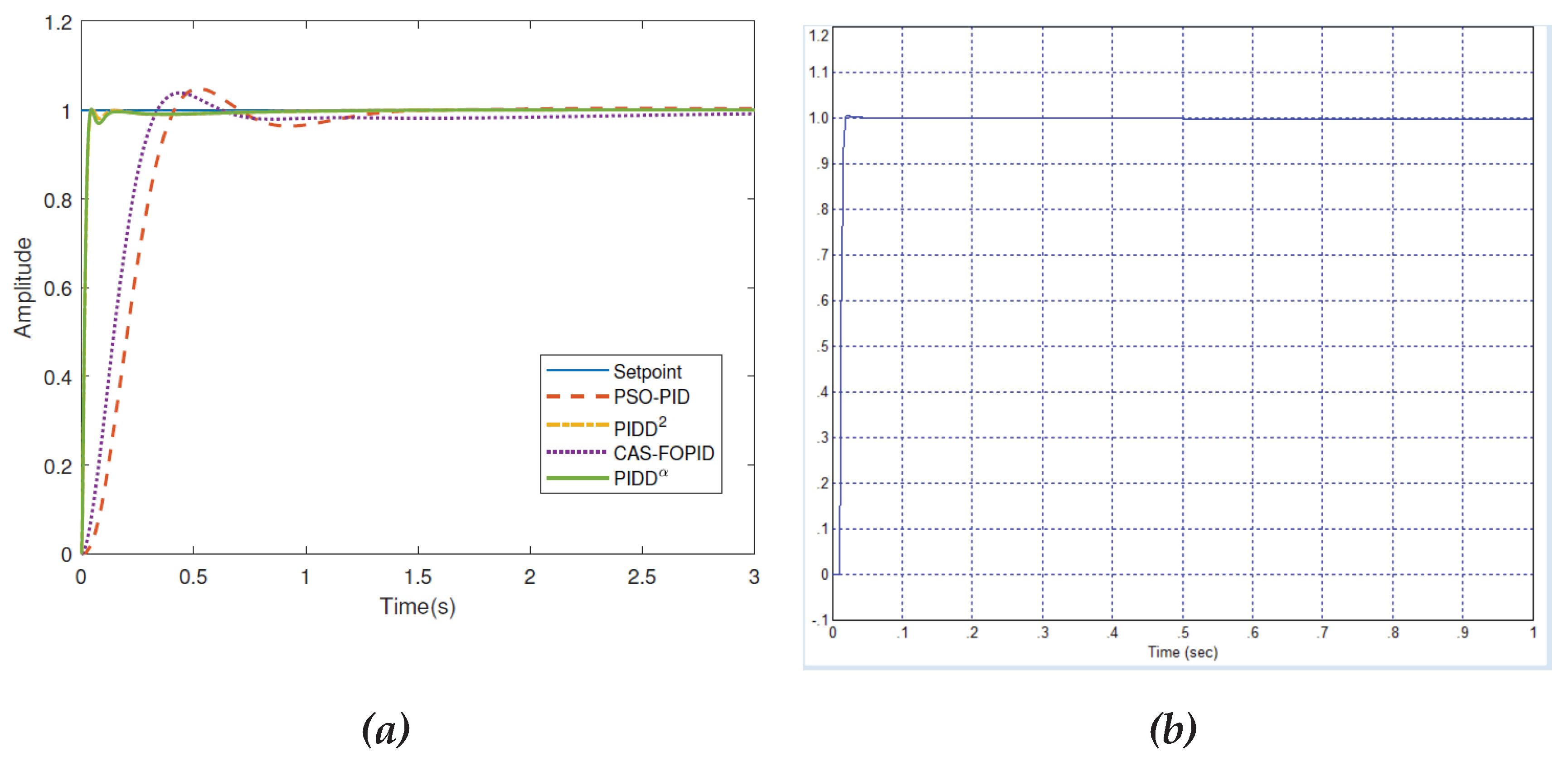
Figure 14.
Project in the VisSim program for modeling the object from Example 4 from the publication [1] and the PID controller, the result in the form of a transient process is shown in Figure 13, b ; rounding the coefficients to 0.1%, as in all our previous results, does not clearly affect the type of transient process (within the line thickness).
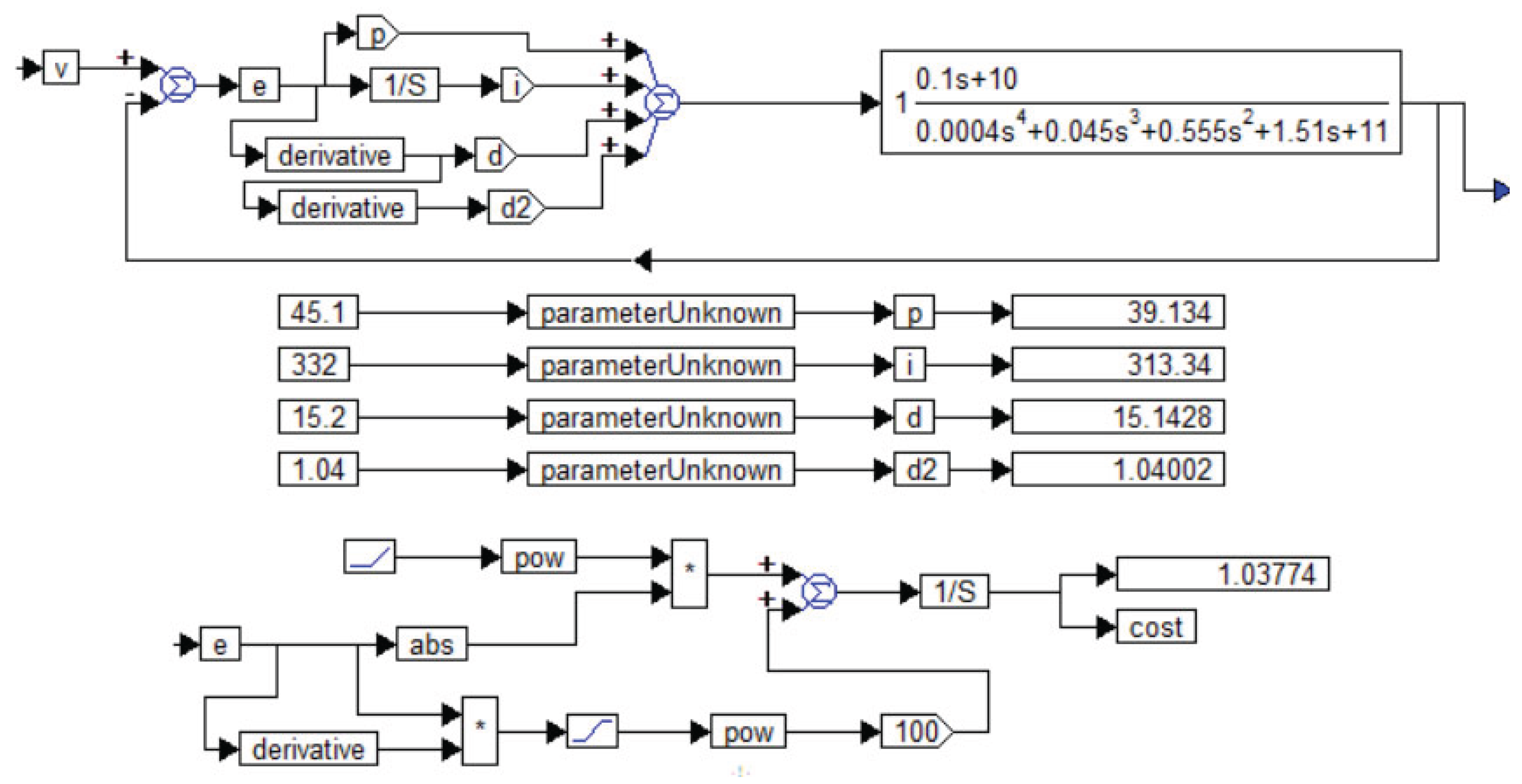
Figure 15.
Comparison of transient processes in objects with transfer functions of the form (19) and (20), from the article [1] (dashed lines), as well as processes in models using the Padé approximation (solid lines), where Figure 15 a refers to model (19) and its approximation, and Figure 15 b – to model (20) and its approximation.
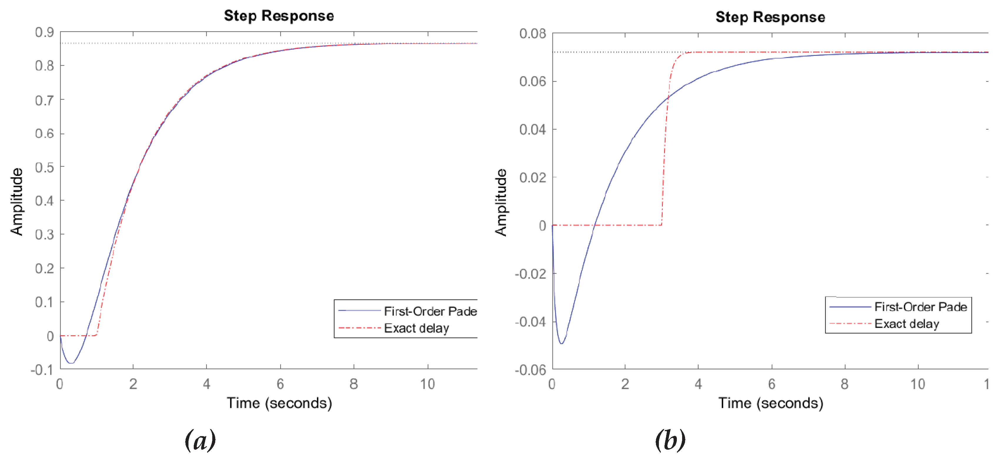
Figure 16.
Comparison of transient processes in objects with transfer functions of the form (19) and (20), from the article [1] with different controllers.
Figure 16.
Comparison of transient processes in objects with transfer functions of the form (19) and (20), from the article [1] with different controllers.
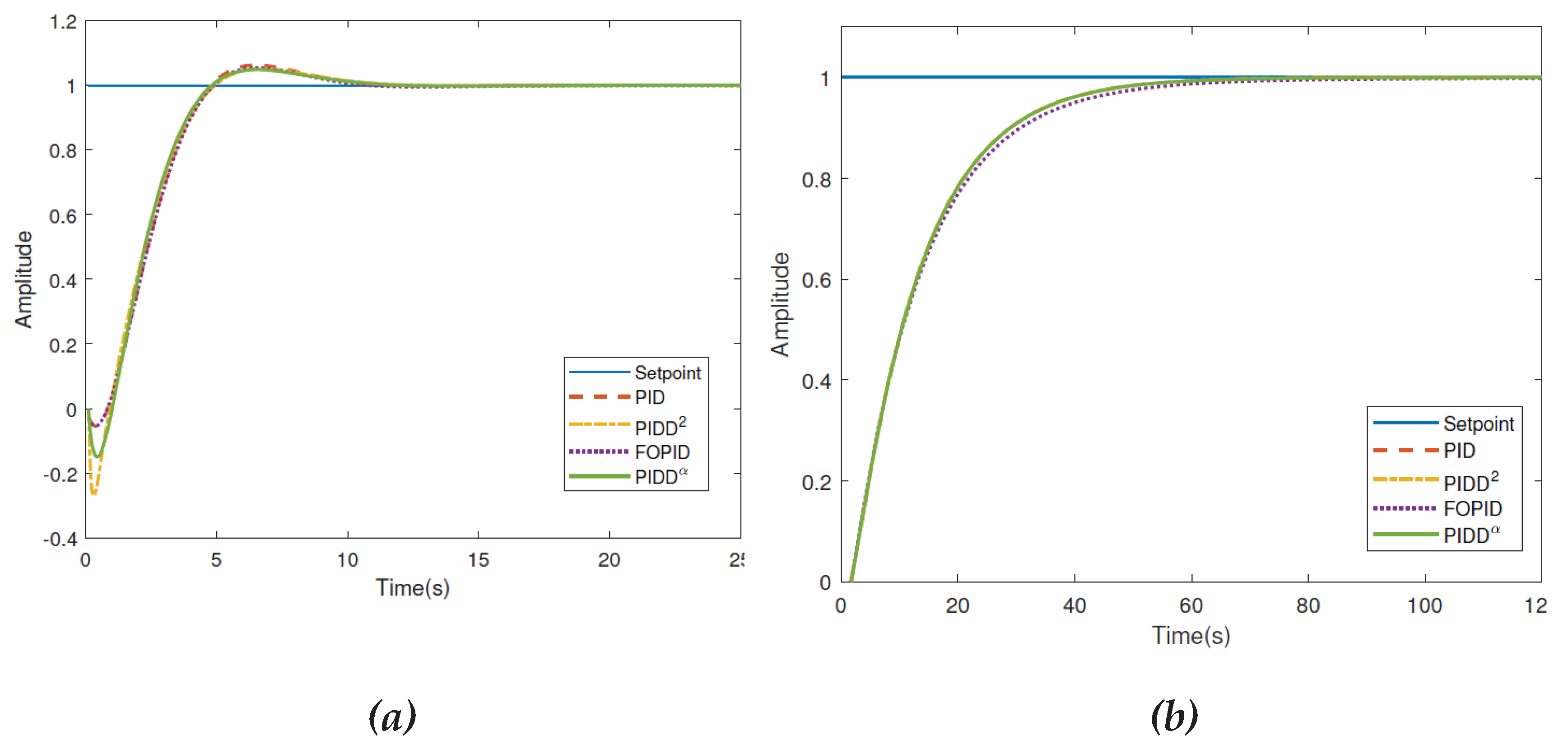
Figure 17.
Comparison of transient processes in objects with transfer functions of the form (19) and (20), from the article [1] with different controllers for a series of four jumps in the task.
Figure 17.
Comparison of transient processes in objects with transfer functions of the form (19) and (20), from the article [1] with different controllers for a series of four jumps in the task.
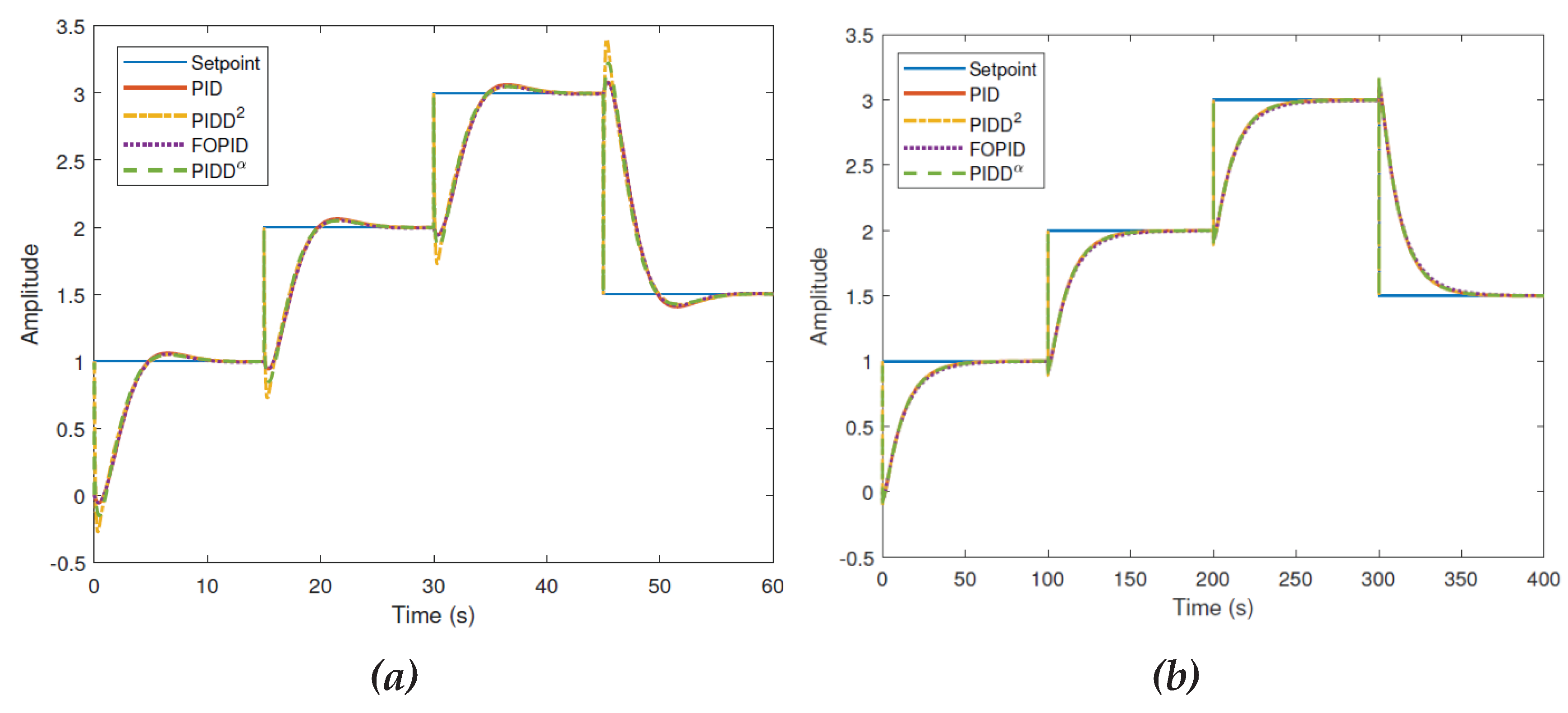
Figure 19.
Project in the VisSim program for optimizing the PID controller for a system with an object (20) from the publication [1] at , the transient process with this controller is shown on the right.
Figure 19.
Project in the VisSim program for optimizing the PID controller for a system with an object (20) from the publication [1] at , the transient process with this controller is shown on the right.
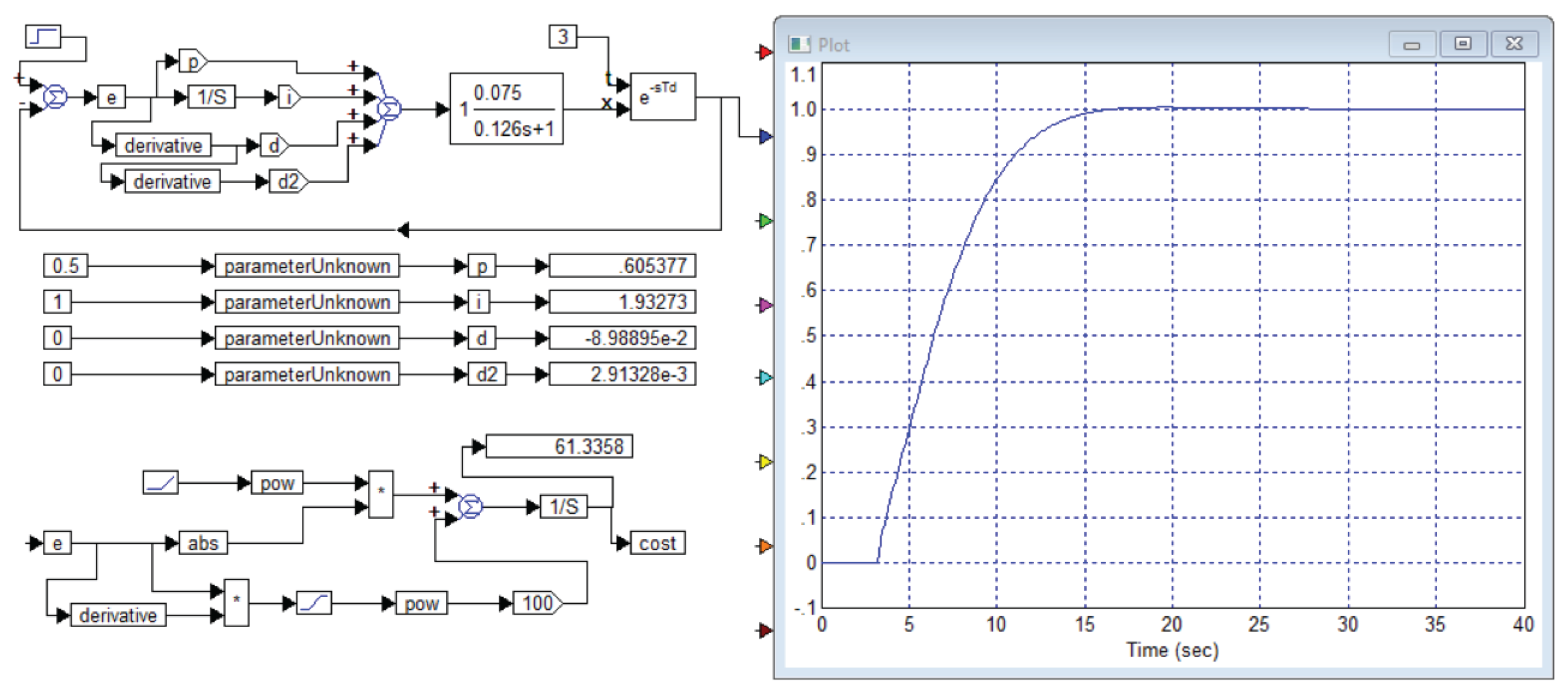
Figure 20.
The structure of the object’s management, which is called in the publication [4] effective and popular, which it is not.
Figure 20.
The structure of the object’s management, which is called in the publication [4] effective and popular, which it is not.
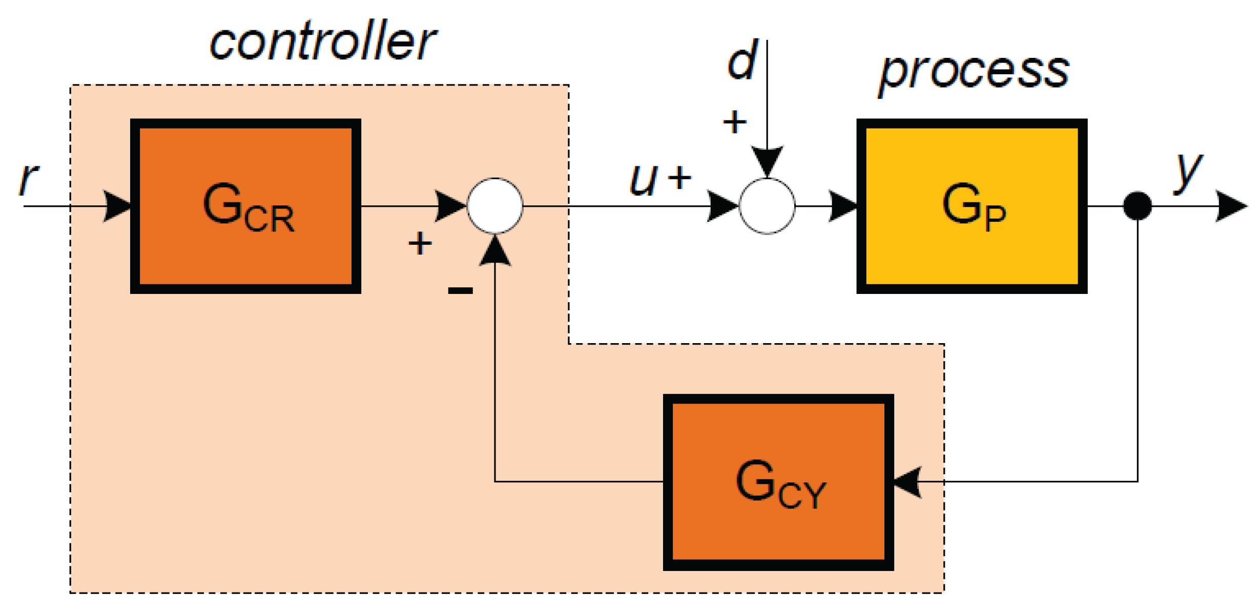
Figure 21.
The only effective and popular structure of object control (obtained by graphic editing of the structure of Figure 20), widely known from the literature.
Figure 21.
The only effective and popular structure of object control (obtained by graphic editing of the structure of Figure 20), widely known from the literature.
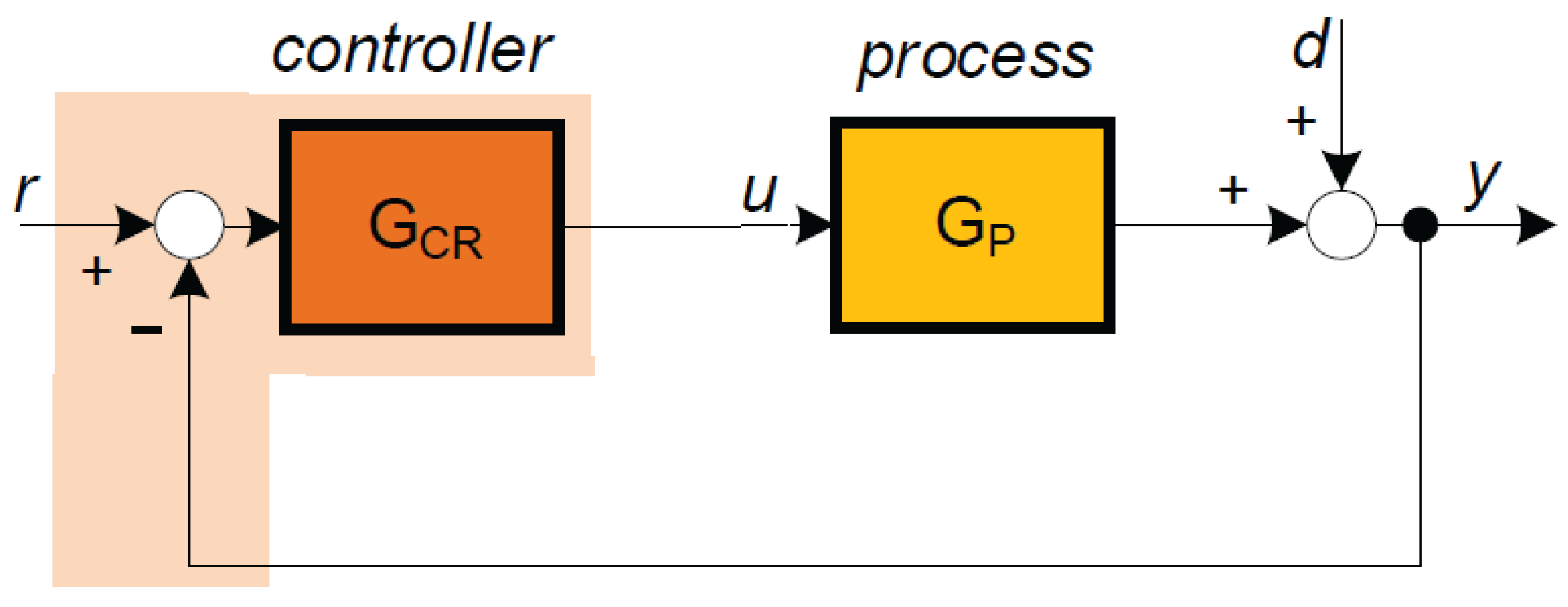
Figure 23.
Comparison of transient processes in the object (20) with our controller (Figure 23a, blue line) and the PIDD2 controller from the article [1], and also in Figure 23b for the latter case a comparison of the process in the system with the controller with (line 1) with the controller with (line 2).
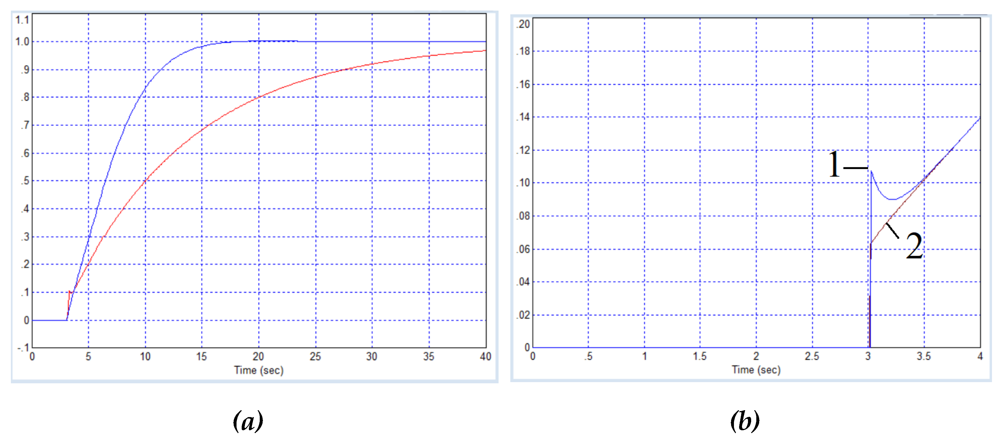

Table 1.
Parameters of various controllers and resulting transient processes from the article [1] for the object from Example 1.
Table 1.
Parameters of various controllers and resulting transient processes from the article [1] for the object from Example 1.
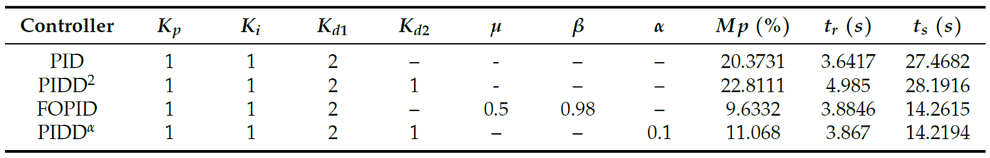 |
Table 2.
Parameters of various controllers and resulting transient processes from article [1] for the object from Example 2.
Table 2.
Parameters of various controllers and resulting transient processes from article [1] for the object from Example 2.
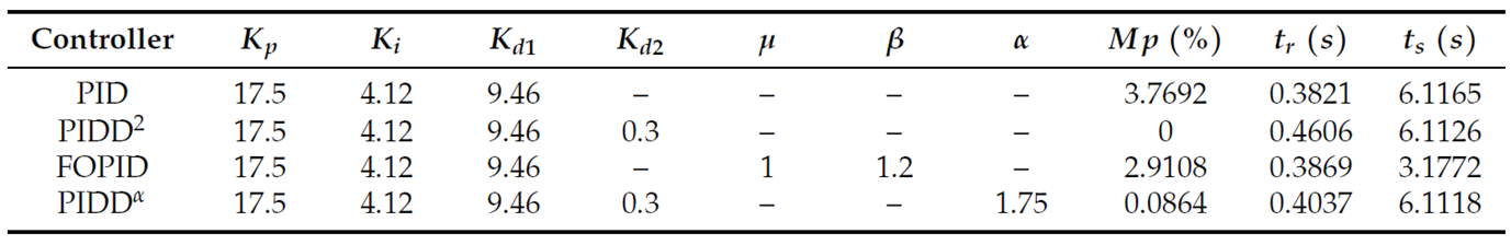 |
Table 3.
Parameters of various controllers and resulting transient processes from article [1] for the object from Example 3.
Table 3.
Parameters of various controllers and resulting transient processes from article [1] for the object from Example 3.
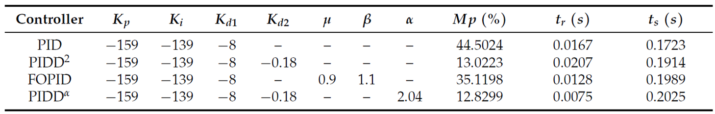 |
Table 4.
Parameters of various controllers and resulting transient processes from article [1] for the object from Example 4.
Table 4.
Parameters of various controllers and resulting transient processes from article [1] for the object from Example 4.
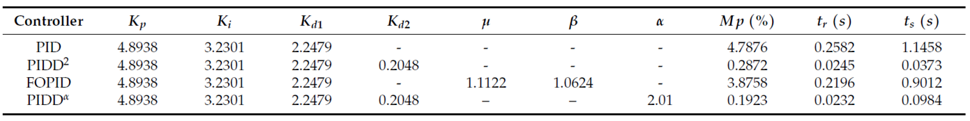 |
Table 5.
Parameters of various controllers and the resulting transient processes from the article [1] for an object from a practical example according to (19).
Table 5.
Parameters of various controllers and the resulting transient processes from the article [1] for an object from a practical example according to (19).
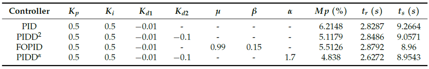 |
Table 6.
Parameters of various controllers and the resulting transient processes from the article [1] for an object from a practical example according to (20).
Table 6.
Parameters of various controllers and the resulting transient processes from the article [1] for an object from a practical example according to (20).
 |
Disclaimer/Publisher’s Note: The statements, opinions and data contained in all publications are solely those of the individual author(s) and contributor(s) and not of MDPI and/or the editor(s). MDPI and/or the editor(s) disclaim responsibility for any injury to people or property resulting from any ideas, methods, instructions or products referred to in the content. |
© 2025 by the authors. Licensee MDPI, Basel, Switzerland. This article is an open access article distributed under the terms and conditions of the Creative Commons Attribution (CC BY) license (http://creativecommons.org/licenses/by/4.0/).
Copyright: This open access article is published under a Creative Commons CC BY 4.0 license, which permit the free download, distribution, and reuse, provided that the author and preprint are cited in any reuse.


