
Submitted:
06 August 2025
Posted:
07 August 2025
You are already at the latest version
Abstract
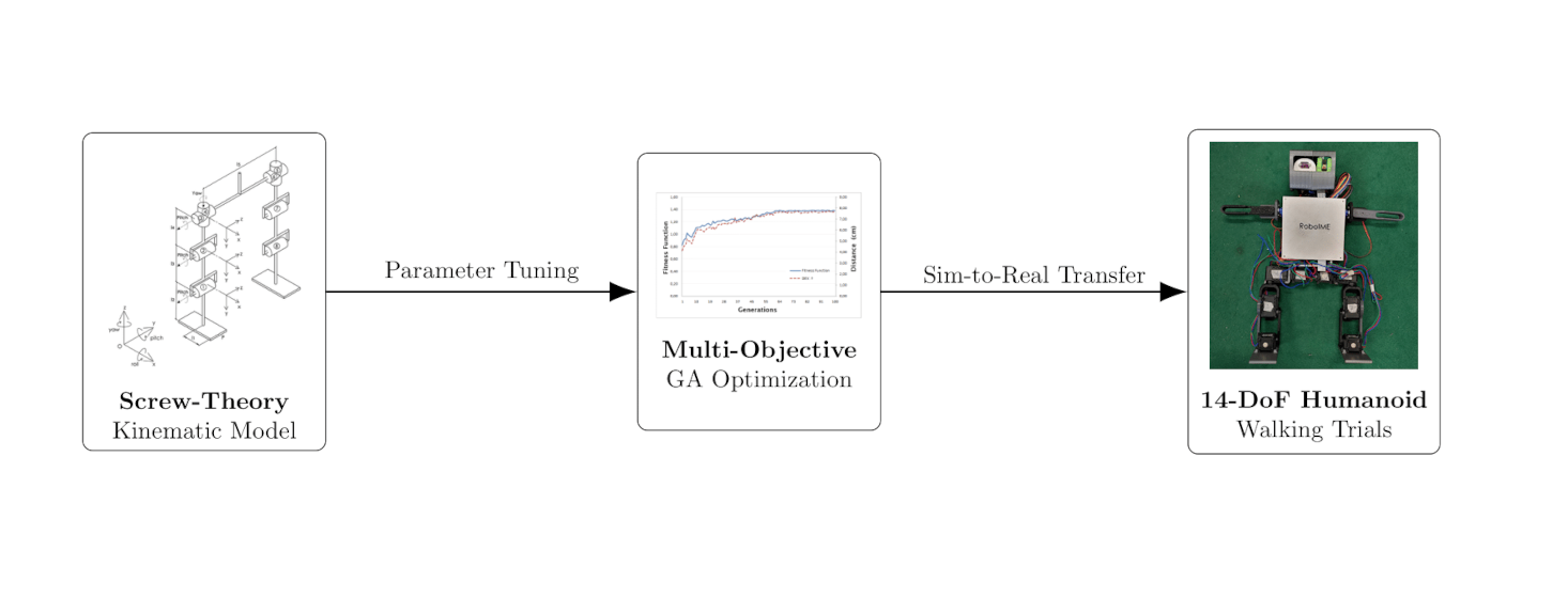
Humanoid bipedal walking remains a challenging problem due to its inherently unstable, high-dimensional dynamics. This paper presents a hybrid framework that matches a compact screw-theory kinematic model with a multi-objective genetic algorithm (GA) for automated gait tuning. By parameterizing the foot’s half-elliptical swing (horizontal and vertical speeds) and the torso pitch angle, our GA optimizes both sagittal stride length and lateral deviation in a single fitness function. We show that the GA reliably converges—achieving plateaued performance by generation 55 and near-optimal trade-offs by generation 100—across runs of up to 500 generations. A Pearson correlation analysis confirms a strong link between fitness and forward displacement ($\rho\approx$ 0.74–0.89) and a moderate link with side‐to‐side drift ($\rho\approx$ 0.57–0.68), highlighting opportunities for refined penalty design. We demonstrate sim-to-real transfer by loading the GA’s best‐found parameters (generation 421) onto a 14 degrees of freedom (DoF) humanoid, which successfully traverses 2 m in five consecutive trials without falling. Compared to traditional Denavit–Hartenberg approaches, our screw-theory formulation reduces parameter count and simplifies Homogeneous Transformation Matrix (HTM) construction, while the GA obviates the need for manual tuning or explicit dynamic equations. This work lays the groundwork for future extensions that incorporate dynamic stability criteria, sensor feedback, and adaptive multi-objective weighting to enhance robustness and efficiency further.
Keywords:
humanoid robot
; screw theory
; inverse kinematics
; genetic algorithm
; gait optimization
1. Introduction
Humanoid robots have emerged as versatile platforms for applications ranging from disaster response to service and industrial tasks. Among the many challenges they face, bipedal locomotion remains particularly demanding due to its high–dimensional, underactuated dynamics and tight stability margins. Classical walking paradigms include passive walkers, which exploit gravity and mechanical design to achieve a low–energy gait at the cost of limited controllability [1]. These semi-passive schemes combine passive dynamics with minimal actuation [2], and fully active approaches relying on servo-driven joints [3]. Of these, active walking has demonstrated the best performance and flexibility on real humanoids such as Atlas and Valkyrie [4,5].
To enhance these methods, model-based controllers—e.g. preview-control of the Zero-Moment-Point (ZMP) [6], Model Predictive Control (MPC) on simplified pendulum models [7], and capture-point feedback [8]—have achieved robust walking even on uneven terrain. Bestmann and Zhang (2022) proposed an open-source omnidirectional gait generator with automated parameter tuning, demonstrating stable multi-direction walking on several humanoid platforms [9]. Wang et al. (2022) leveraged a decoupled actuated SLIP model and high-frequency MPC to traverse challenging ground with minimal perception [7]. Hu et al. (2023) provide a comprehensive survey of modern bipedal control methods, highlighting the enduring utility of reduced-order, model-predictive strategies alongside emerging learning-based techniques [10].
Evolutionary algorithms, particularly Genetic Algorithms (GAs), offer a complementary route by automatically discovering gait parameters in large, nonlinear search spaces without explicit dynamic models [11]. Szabó (2023) showed that a GA can evolve a humanoid’s joint trajectories to achieve both stable walking and autonomous fall recovery, drawing inspiration from infant learning [12]. Gupta et al. (2024) applied a multi-objective GA (NSGA-II) on a NAO robot to balance energy efficiency and stability margin, extracting Pareto-optimal gait sets for hardware validation [13]. More recently, Chagas et al. (2024) combined a screw-theory kinematic model with a GA to tune swing-leg trajectories and torso pitch, converging within 100 generations and successfully transferring the gait to a 14-DoF humanoid for 2 m open-loop trials [14].
Accurate kinematic modeling is essential for both model-based and evolutionary schemes. Screw theory offers a compact alternative to the classic Denavit–Hartenberg (DH) method, reducing the parameter count and simplifying the construction of Homogeneous Transformation Matrices [15,16]. Zhong et al. (2023) fused screw and DH formulations to derive real-time inverse kinematics for a 7-DoF humanoid arm, improving end-effector accuracy by over 70 % in hardware tests [17]. Sun et al. (2023) used Product-of-Exponential (POE) screw modeling to plan stable gaits for a novel hybrid biped mechanism, validating the approach in simulation [18].
Finally, real-world validation remains the gold standard. Radosavovic et al. (2024) demonstrated zero-shot sim-to-real walking with a transformer-based policy on a full-size humanoid, achieving robust locomotion over outdoor terrain without online retraining [19]. These advances underline the need for hybrid frameworks that couple accurate, screw-theoretic kinematics with automated optimization to produce stable, efficient humanoid gaits deployable on real hardware.
This paper presents such a framework. Section 2 derives our screw-theory kinematic model and HTM construction. Section 3 details the multi-objective GA for tuning leg-swing speeds and torso angle. Section 4 describes our simulation and 14-DoF hardware setup. Section 5 reports convergence analyses, correlation metrics, and sim-to-real trials. Section 6 discusses insights and limitations, and Section 7 concludes with future directions.
2. Mathematical Formulation
2.1. The Kinematic Model of the Robot
Figure 1 shows the kinematic structure of the lower limbs of the humanoid. The legs of the robot are composed of revolution joints with four degrees of freedom each, being 2 DoF on the hip and thigh, 1 DoF on the knee, and 1 DoF on the ankle.
2.2. Formulating the Kinematic Equations
Before starting the kinematic equations formulation, it is necessary to define the movement restrictions and plan the joints movement. The initial conditions for obtaining the kinematics, in this work, are: the upper part of the body mass is concentrated in the center of the robot; the CoM of the robot is in a fixed-height plane; there is enough friction for the robot not to slip; the gait happens in one single direction; there is no interference from external forces, such as: collisions with other bodies; the joints are collision-free and the contact surface is flat.
Having defined the restrictions, the second step is to determine how the movement will be performed. That said, the planning of the movement happens as follows: initially, one of the legs of the robot is fixed and serves as a reference axis for the leg that is moving. The objective is to calculate the angular variation and the joints velocity of the moving leg from the speeds of the final effector (point p in Figure 1) which is the foot of the robot. After the leg that started the movement lands on the ground, it becomes the reference and the leg that was at rest starts to move. The process is repeated until it finds a stop condition.
The extraction of the direct kinematic follows the sequence as indicated by the following Algorithm 1 procedure:
| Algorithm 1 |
|
2.3. Choose a Fixed Coordinate System
In Figure 1, the fixed coordinate system is centered on the origin of the foot of the robot. The axis z points to the head of the robot, the x-axis is in the direction of the sagittal plane, and the y-axis is towards the frontal plane.
2.4. Identify Bodies, Joints and Axis
The joints of the robot are indicated by the numbers 1 to 8. The numbers 1, 2, 3, and 4, respectively, indicate the joints of the ankle, knee, hip rotation, and thigh flexion of the right leg. The joints 8, 7, 6, and 5 represent the joints of the ankle, knee, hip rotation, and flexion of the left leg. It is possible to identify the orientation of the joint axes through the Fleming Rule.
2.5. Identify the Screw Parameters
Table 1 shows the indication of the screw parameters , , and the axes distances to the referred joints indicated by , and , in relation to the fixed coordinate system.
2.6. Build the HTM of Each Joint, as Well as the Matrix with the Reference Location of the End Effector
Note: The terms , and refer to prismatic joints; as all joints are of revolution, they are eliminated from the equation 4.
The final transformation is given by equation 5, where corresponds to the position of the foot of the robot.
2.7. Apply the SSDM with the HTM of Each Joint
2.8. Multiply the SSDM Result by the Matrix of End Effector
The final transformation is obtained by multiplying the matrix by the matrix of final transformation, see equation 7.
2.9. Inverse Kinematics
In inverse kinematics, the objective is to find the equations that make it possible to relate the linear and angular speeds of the End Effector, that is, of the foot of the robot, as a function of the speeds of the joints itself.
Letting the vector that contains the angular and linear speeds, see equation 12.
The joint speed vector is represented by equation 13.
The relation between and q described in [15] is given by equation 14.
where in is the Jacobian described by equation 15
Being that and represent the angular and linear speeds, respectively. Knowing the speeds of the tool, the objective is to find the speeds of the joints, which can be obtained by applying equation 16.
2.10. Trajectory Model of the Robot Foot
Assuming that the foot of the humanoid performs an elliptical movement, the velocities vector is given by equation 17.
where, the horizontal linear speed, equation 18, and is the linear vertical speed, equation 19, of the foot of the robot.
where, mf is the engine rotation frequency, is given by equation 20, axf and azf are input parameters for speed adjustment. vgait is the speed of the gait.
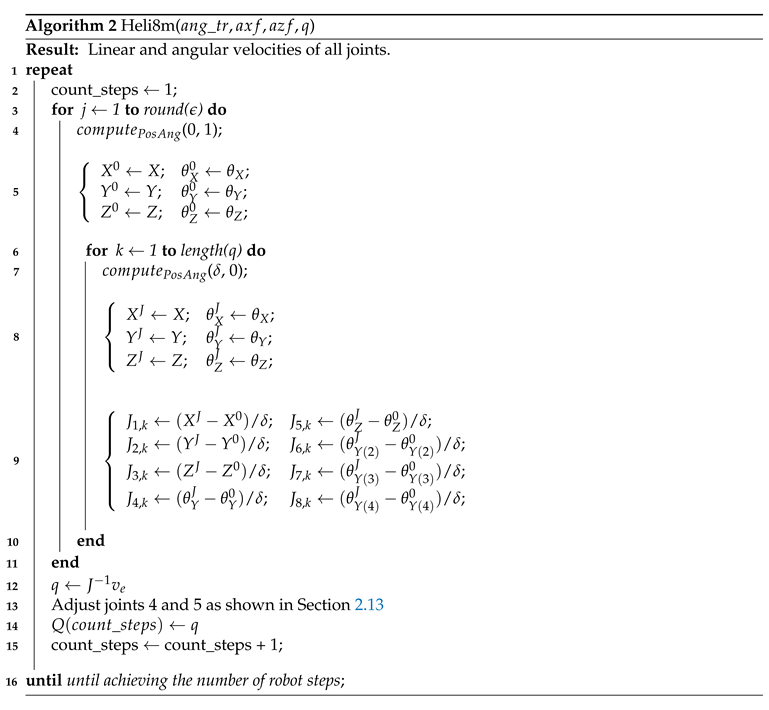
2.11. Jacobian Matrix
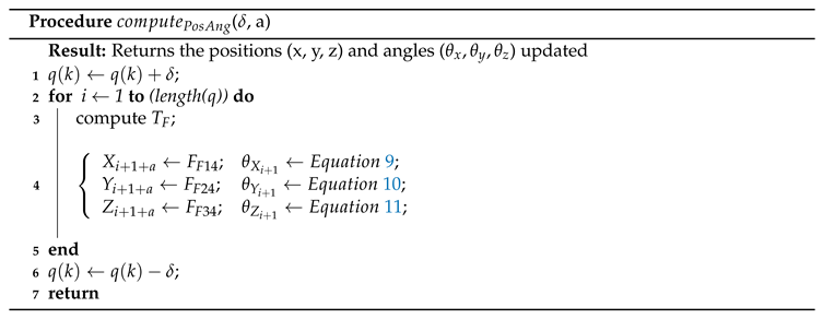
The Heli8m() procedure takes ang_tr, axf, azf, cont_steps, and the velocity vector q as parameters. On line 2, cont_step receives 1, and the program begins execution. In line 3, the program executes a loop that varies from 1 to . In line 4, the system calls . This procedure obtains the x, y and z position values, and the , , and angle values of the joints. The parameter serves to help calculate the partial derivatives of the Jacobian matrix, and the parameter a serves to adjust the indexes of the position and velocity vectors. Line 9 shows the obtainment of the Jacobian matrix by applying the definition of Derivative. In line 12, the vector q receives the product of the inverse Jacobian matrix by the velocity vector of the final effector. Next, there is the adjustment of joints 4 and 5, which rotate the hip. In line 14, the system updates the matrix Q, which contains all the information about the speed of the joints during the steps. Finally, the procedure updates the value of cont_steps in line 15 and it checks if the program has reached the final; if so, the system stops; if it does not, it reruns the loop from line 3.
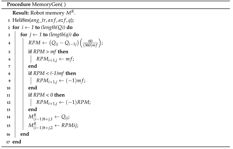
2.12. Robot Memory File
The MemoryGen( ) procedure is responsible for generating the memory of the robot. Initially, it calls Heli8m() procedure, and then in line 2, it traverses a for ranging from 2 to the end of Q matrix. In line 3, the procedure loops through vector q, which calculates the value of motor rotation frequency (RPM), line 4. In line 5, the program checks if the value found exceeds the frequency of motors mf, and if so, RPM receives the value of mf. If the RPM value is less than the lower limit that the engine supports, RPM receives (-1)mf, which is the minimum mf value. In line 11, the program checks if the RPM value is negative; if so, RPM receives the RPM module. Finally, the system generates the MR memory matrix that contains the values of the angular positions and rotation frequency of the motors for each robot joint during the steps.
2.13. Hip Rotation
The hip rotation is an input parameter, this allows you to simplify two degrees of freedom to obtain the reversible kinematics and obtain a Jacobian matrix. This parameter variation is made by adjusting the angles of joints 4 and 5 and follows equation 21.
where, indicates the step number of the robot.
3. The Algorithm
Figure 2 shows the flowchart of the proposed algorithm. Initially, the system is configured as indicated by the Set Inputs block. Then, the system checks whether it is an initial execution or not; if it is the first execution, the system loads the initial population and calculates the inverse kinematics. After the calculus, the system checks whether the parameters are suitable or not, in other words, whether the robot has fallen or not. With the information from the kinematic calculation and the platform behavior, the system calculates the value for the fitness function. The genetic algorithm parameters are adjusted, which means the surviving individuals are used as an entrance for a new generation. The completion of the process occurs when the number of predefined generations is reached.
3.1. The GA Encoding
This work uses the real value representation for genes because it is a continuous distribution rather than a discrete one. Therefore, consider the vector with to be the genotype for a solution with k genes. Figure 3 illustrates a chromosome with three genes, where the genes at locus 1, 2, and 3 represent the robot trunk tilt angle, robot foot horizontal velocity, and robot foot vertical velocity, respectively.
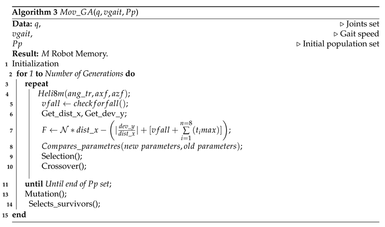
The pseudocode for algorithm 3 takes the set of joints of the robot as input, the walking speed and the initial population, being formed by the set containing the inclination of the trunk and the foot of the robot horizontal and vertical speeds. The output is a list containing the axf, azf and ang_tr optimized values for each generation.
In line 1, the system initializes all variables and proceeds to line 3, where it enters a repetition structure that will be executed until reaches the total number of predefined generations. In line 4, the program calls the Heli8m() function, which is responsible for solving the inverse kinematics of the humanoid. In line 5, the checkforfall () function returns to fall condition, if the robot falls, the vfall variable receives 1 as the value, otherwise, it receives 0, see equation 22.
In line 6, Get_distx and Get_devy are responsible for accessing the displacement values in the sagittal plane and the lateral deviation suffered by the robot during the step. Line 7 shows the calculation of the fitness function F, which is composed of two parts, reinforcement and penalty. The reinforcement part consists of the product between the N factor and the distance roamed in the sagittal plane. The N factor is an estimate given by equation 23. N assumes the maximum value that can be reached by the penalty; this way, the system ensures that any positive displacement will be rewarded. Equation 24 shows the relation between the deviation suffered by the robot due to its displacement. Equation 25 portrays the penalty ratio, in case the servomechanisms torques exceed the maximum allowed. The determination of the maximum value, where indicates the N floor and represents the maximum torque of the servomechanism associated with the joint i.
In line 8, the function Compares_Parameters checks whether the new parameter is better than the previous one. If better, the algorithm keeps the new value, otherwise, the function discards it. In line 9, the algorithm calls the Selection() function through the roulette method. Then, the system executes the Crossover( ) function. After roaming through the entire population, the chromosomes undergo Mutation. In line 14, the Select_survivors() function will contain the new generation individuals. The system continues the execution until it reaches the number of generations predefined at the beginning of the program.
The algorithm of the Crossover( ) procedure describes the sequence of steps for the achievement of crossover between chromosomes. The crossover is made between the axf, azf and ang_tr genes. Initially, the procedure identifies the chromosome with highest aptitude and the lowest aptitude – both are removed from the potentially partners list. Then the system seeks a random partner and matches it with the best element. The result of the crossover substitutes the most weak chromosome.
| Procedure Crossover( ) |
| Result: New chromosome |
| 1 Identifies the chromosome with the highest fitness |
| 2 Identifies the chromosome with the lower fitness |
| 3 Removes and from the suitors list |
| 4 Identifies a potential partner among the rest of the population |
| 5 Returns with to the list of population |
| 6 The new chromosome is given by: ; |
The algorithm of theMutation( ) procedure shows the function that realizes the chromosomes mutation. The entire population set is covered; the best individuals are excluded of the process, characterizing the process of elitism. The mutation rate is given by equation 26, where n{BC} is the number of elements belonging to the set of the best chromosomes and n{Pp} is the number of elements belonging to the set of population .

4. Experimental Setup
The test of the algorithm has four steps, namely: first, IV-A) 3D modeling of the mechanism; second, IV-B) development of the real platform; third, IV-C) development of a simulator for the proposed model; fourth, IV-D) algorithm implementation.
4.1. 3D Model
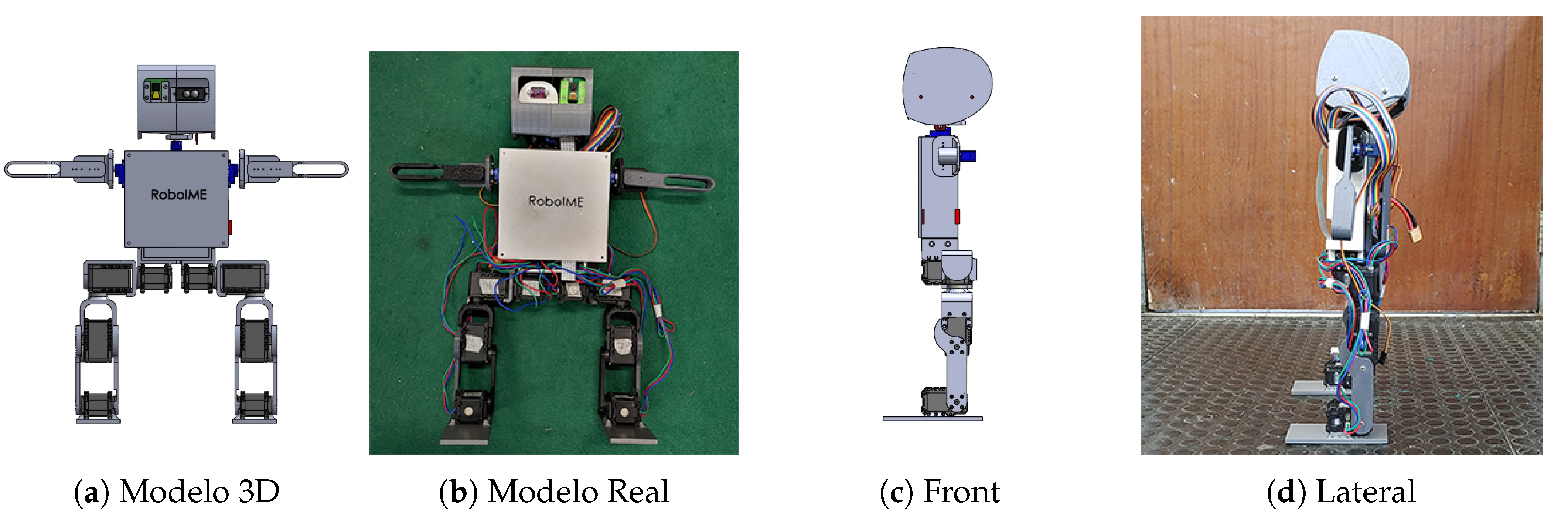
The 3D model of the robot has 14 degrees of freedom distributed as follows: 2 GDL for the right and left ankles, 2 GDL for the right and left knees, 2 GDL for the right and left thighs, 2 GDL for the right and left hips, 4 GDL for the right and left shoulders and 2 GDL for the neck. Using SolidWorks 2020 allowed the modeling and testing of all platform parts before fabrication. Fig. 3a shows the 3D humanoid model.
Figure 4.
Plataforma Humanoide 3D
4.2. Real Platform Model
The real robot model comes from the 3D model. The robot fairing was 100% printed, which facilitated the construction and made the project feasible. The engines used for the legs are Dynamixel AX-12A servomotor and for the arms and neck SG90 engines. The platform operates with a Raspberry Pi 4 board for signal and image processing and a myRio board for interfacing with the engines. The hardware has an inertial sensor, a mini Lidar distance sensor, and a camera to interface with the environment. Figure 3b shows the real platform.
4.3. Simulator
Figure 5, shows the graphical interface for the simulator, it is composed of the model coming from SolidWorks and the Simulink Contact Force Library, version 5.0. In short, the simulator consists of a graphical interface where it is possible to monitor the simulation by moving the robot on a path. The algorithm interfaces with the objects provided by the Simulink and, in this way, captures the information of the forces acting on the joints and on the ground. The realism of the simulation depends on the input parameters, such as the friction provided by the surface and the correct sizing of the pieces and robot components. As a way out, a data is generated containing the related information to the joints positions and engines frequencies. This file will serve as a memory for the real robot. Besides this memory, information regarding the behavior of the humanoid joints is generated.
4.4. Algorithm Implementation
The algorithm was implemented in the MatLab programming language, version R2019b. It integrates the graphical elements of the 3D robot model with the Simscape Multibody Contact Forces Library, made available by MatLab. The program was divided into modules to facilitate the removal of each function in case tests are necessary. For instance: it is possible to perform the kinematic calculation procedure of the robot separately, or remove some of the functions of the genetic algorithm, like Mutation( ), Selection(), and Crossover( ). Table 2 shows the initial population used as input for the algorithm. is the angle of the torso inclination, e are the linear speeds on the x and z axes, according to the reference in Figure 1.
The experiments began with the selection of the initial population and proceeded to execute the algorithm—varying the number of generations while maintaining that population with . The simulation required an Intel(R) Xeon(R) CPU CPU E5-1650 0 processor, with 3.20GHz clock, 16 GB of RAM, and an NVIDIA GF108GL [Quadro 600] graphics card. The simulation runs over Operating System Linux Ubuntu 18.04.5 LTS. Figure 6 graphically shows the sequence of movements that the humanoid performs to accomplish a complete gait cycle. Initially, the robot is inert with its feet parallel. Next, it steps forward with its left leg and rotates the hips to the right. After the rotation, the robot rests its left foot on the ground and performs the opposite movement, moving forward with its right leg. Section 5 shows the graphical analysis of the results obtained with the execution of the algorithm by varying the number of generations. The simulation uses a fixed population of 10 individuals and varies the generations in number. The experiment starts running with 50 generations; after the first execution, it starts to increment the generations by 50, up to 250. The last test used a population of 500 generations. For each set of generations, the section uses the Pearson correlation matrix to verify the strength of the association between variables.
5. Results
In this section, we present a comprehensive evaluation of the proposed gait-optimization algorithm. We begin by demonstrating the global convergence behavior of the genetic algorithm over a long run (500 generations), then examine how varying the number of generations (50, 100, and 500) affects both the fitness and lateral deviation. Next, we consolidate these observations via a correlation analysis and identify the single best individual (generation 421) for deployment. With the optimal parameters in hand, we analyze detailed joint trajectories and center-of-mass motion over eight gait cycles in simulation, and finally validate the approach on the real 14-DoF humanoid platform, showing successful 2 m trials without falls.
5.1. Global Convergence (500 Generations)
Figure 7 shows the evolution of the fitness and lateral deviation over 500 generations. Note how both curves plateau by generation 55, indicating that the GA has converged.
5.2. Effect of Generation Count
5.3. Consolidated Correlation Analysis and Best Individual Choice
Table 3 aggregates Pearson correlations for 50, 100 and 500-generation runs. We see high fitness–distance correlations throughout, while fitness–deviation remains moderate.
Choosing the Best Individual: The peak fitness occurs at generation 421 in the 500-gen run, with deviation only 6.84% above its minimum (found at 150 gens).
5.4. Joint Trajectories (8 Gait Cycles)
Figure 10 plots the optimized joint angles and CoM over eight consecutive steps. Note the rapid settling of ankle and knee after the first cycle, and the nearly constant CoM height.
5.5. Real-Platform Validation
Finally, we loaded the gen. 421 parameters onto the physical 14-DoF humanoid, which successfully walked 2 m in 5/5 trials without falling. Figure 11 shows key frames from start (a–c), middle (d–f) and end (g–i) of one demonstration.
6. Discussion
In this work we have presented a hybrid approach to humanoid gait generation that combines a compact screw-theory kinematic model with a multi-objective genetic algorithm (GA). By exploiting screw parameters instead of the more common Denavit–Hartenberg formulation, we reduced the number of model parameters and simplified the HTM construction, yet still achieved accurate forward and inverse kinematics for a 14-DoF biped.
Our simulation results (Section 5) demonstrate that the GA converges reliably within the first 100–150 generations in terms of overall fitness (step length) and lateral deviation, and fully stabilizes by generation 55 in a 500-gen run (Fig. 7). The high Pearson correlation between fitness and sagittal distance (–) confirms that our objective function successfully rewards long steps, while the moderate correlation with lateral deviation (–) highlights a residual bias toward sacrificing some stability for stride length.
By inspecting all six population-duration scenarios (50, 100, …, 500 generations), we identified generation 421 of the 500-gen run as the best compromise: it attains the highest fitness while keeping deviation within 6.8% of the minimum observed at 150 generations (Table 3). Deploying these parameters on the real robot yielded consistent 2 m trials without falls (Fig. 11), validating the transferability of our solutions from simulation to hardware.
Despite these strengths, several limitations remain. First, our current penalty term for lateral deviation—proportional to —proved only moderately effective. Future work should explore alternative multi-objective schemes (e.g. Pareto-based GA [18]) or dynamic weighting strategies that more aggressively penalize side-to-side drift.
Moreover, we assumed constant friction and neglected inter-joint compliance; extending the model to include joint elasticity, ground compliance and energy consumption metrics would yield a more holistic optimization. Likewise, adding upper-body motion as extra genes (e.g. arm swing, torso yaw) could both improve balance and reduce energy costs, aligning with human-inspired gait strategies [12].
Finally, while screw-theory offered a concise way to derive kinematics, future implementations could incorporate dynamic stability criteria—such as zero-moment-point (ZMP) or divergent component of motion (DCM) control—within the GA loop, enabling simultaneous optimization of kinematics and dynamics.
In summary, our hybrid screw-kinematics + GA framework provides a flexible, model-based learning approach to humanoid walking. With targeted enhancements to the fitness formulation, feedback integration, and dynamic modeling, this methodology has strong potential to produce stable, efficient gaits across a wide range of tasks and terrains.
7. Conclusions
We have introduced a hybrid gait-generation framework that combines a compact screw-theory kinematic model with a multi-objective genetic algorithm to tune humanoid walking parameters automatically. By parameterizing the foot’s half-elliptical swing speeds and the torso pitch angle, our GA simultaneously maximizes sagittal stride length and minimizes lateral deviation. Simulation results demonstrate reliable convergence—plateauing by generation 55 and yielding near-optimal trade-offs by generation 100—across runs of up to 500 generations, with strong correlations between fitness and forward displacement ( 0.74–0.89) and moderate correlations with side-to-side drift ( 0.57–0.68).
We identified generation 421 of a 500-gen run as the best compromise and validated these parameters on a 14-DoF humanoid, which successfully walked 2 m in five consecutive trials without falling. Compared to Denavit–Hartenberg-based methods, our screw-theory formulation reduces the parameter count and streamlines the construction of HTMs. At the same time, the GA obviates the need for manual tuning and explicit dynamic equation solving.
In future work, we will refine the lateral deviation penalty—potentially via Pareto-based or dynamic-weighting schemes—and integrate real-time sensor feedback (IMU, foot pressure) to enable closed-loop adaptation over uneven terrain. Incorporating upper-body motion, energy consumption metrics, and dynamic stability criteria (e.g., Zero-Moment Point, ZMP) directly into the GA fitness function will further enhance robustness and efficiency.
Author Contributions
Conceptualization, F.S.C. and P.F.F.R; methodology, F.S.C.; software, F.S.C. and L.D.P.F; validation, F.S.C., L.D.P.F and P.F.F.R; formal analysis, F.S.C. and P.F.F.R; investigation, F.S.C. and P.F.F.R; resources, F.S.C and P.F.F.R; data curation, F.S.C..; writing—original draft preparation, F.S.C, P.F.F.R; writing—review and editing, F.S.C, M.M.L.F and P.F.F.R; visualization, F.S.C and M.M.L.F; supervision, P.F.F.R; project administration, P.F.F.R; funding acquisition, P.F.F.R. All authors have read and agreed to the published version of the manuscript.
Funding
This research was financed in part by CAPES - Brazil - Finance Code 001 and grant 88881.505193/2020-01
Acknowledgments
The authors would like to express their gratitude to Professors Antonio L. L. Ramos and Aurilla Aurelie Arntzen Bechina for their invaluable guidance, and to undergraduate students Franciele Sembay, José Lauro O. Schramm, Gabriel M. Lima, Ana L. Buze Silva, and Mateus S. Carvalho for their contributions to this project.
Conflicts of Interest
The authors declare no conflicts of interest.
References
- McGeer, T. Passive Walking with Knees. In Proceedings of the Proceedings of the IEEE International Conference on Robotics and Automation, 1990, Vol. 3, pp. 1640–1645. [CrossRef]
- Hirayama, K.; Hirosawa, N.; Hyon, S. Passivity-Based Compliant Walking on Torque-Controlled Hydraulic Biped Robot. In Proceedings of the 2018 IEEE-RAS 18th International Conference on Humanoid Robots (Humanoids), 2018, pp. 1–6. [CrossRef]
- Kajita, S.; Benallegue, M.; Cisneros, R.; Sakaguchi, T.; Morisawa, M.; Kaminaga, H.; Kumagai, I.; Kaneko, K.; Kanehiro, F. Position-Based Lateral Balance Control for Knee-Stretched Biped Robot. In Proceedings of the 2019 IEEE-RAS 19th International Conference on Humanoid Robots (Humanoids), 2019, pp. 17–24. [CrossRef]
- Wiedebach, G.; Bertrand, S.; Wu, T.; Fiorio, L.; McCrory, S.; Griffin, R.; Nori, F.; Pratt, J. Walking on partial footholds including line contacts with the humanoid robot atlas. In Proceedings of the 2016 IEEE-RAS 16th International Conference on Humanoid Robots (Humanoids), 2016, pp. 1312–1319. [CrossRef]
- Wang, M.; Wonsick, M.; Long, X.; Padr, T. In-situ Terrain Classification and Estimation for NASA’s Humanoid Robot Valkyrie. In Proceedings of the 2020 IEEE/ASME International Conference on Advanced Intelligent Mechatronics (AIM), 2020, pp. 765–770. [CrossRef]
- Kajita, S.; Kanehiro, F.; Kaneko, K.; Fujiwara, K.; Harada, K.; Yokoi, K.; Hirukawa, H. Walking Pattern Generation by Preview Control of Zero-Moment Point. In Proceedings of the Proc. IEEE International Conference on Robotics and Automation (ICRA), 2003, pp. 1620–1626. [CrossRef]
- Wang, K.; Wonsick, M.; Long, X.; Padir, T. Fast Online Optimization for Terrain-Blind Bipedal Robot Walking with a Decoupled aSLIP Model. Frontiers in Robotics and AI 2022, 9, 812258. [CrossRef]
- Jeong, H.; Sim, O.; Bae, H.; Lee, K.; Oh, J.; Oh, J.H. Biped walking stabilization based on foot placement control using capture point feedback. In Proceedings of the 2017 IEEE/RSJ International Conference on Intelligent Robots and Systems (IROS), 2017, pp. 5263–5269. [CrossRef]
- Bestmann, M.; Zhang, J. Bipedal Walking on Humanoid Robots through Parameter Optimization. In Proceedings of the RoboCup Symposium, 2022, pp. 1–8.
- Hu, C.; Cheng, T.; Liu, X.; Zhao, J. An Overview on Bipedal Gait Control Methods. IET Collaborative Intelligent Manufacturing 2023, 5, e12080. [CrossRef]
- Holland, J.H. Adaptation in Natural and Artificial Systems: An Introductory Analysis with Applications to Biology, Control and Artificial Intelligence; MIT Press: Cambridge, MA, USA, 1992.
- Szabó, R. Design Approach for Evolutionary Techniques Using GAs: Application for a Biped Robot to Learn to Walk and Rise after a Fall. Mathematics 2023, 11, 2931. [CrossRef]
- Gupta, P.; Pratihar, D.K.; Deb, K. A Knee-Based Multi-Objective Optimization for Gait Cycle of 25-DOF NAO Humanoid Robot. In Proceedings of the Advances in Mechanical Engineering (Springer). Springer, 2024, pp. 47–62.
- Chagas, F.S.; de Farias, L.D.P.; Bechina, A.A.A.; Ramos, A.L.L.; Rosa, P.F.F. Walking Optimization Algorithm for Humanoid Robots Using Genetic Algorithm. In Proceedings of the 2024 10th International Conference on Control, Decision and Information Technologies (CoDIT), 2024, pp. 2348–2353. [CrossRef]
- Tsai, L.W. Robot Analysis and Design: The Mechanics of Serial and Parallel Manipulators, 1st ed.; John Wiley & Sons, Inc.: USA, 1999.
- Lynch, K.M.; Park, F.C. Modern Robotics: Mechanics, Planning, and Control, 1st ed.; Cambridge University Press: USA, 2017.
- Zhong, F.; Wang, T.; Li, Y. IK Analysis of Humanoid Robot Arm by Fusing DH and Screw Theory to Imitate Human Motion. IEEE Access 2023, 11, 66730–66740. [CrossRef]
- Sun, P.; Zhou, J.; Li, Z. Screw-Theoretic Modeling and Gait Planning for a Novel Hybrid Biped Leg Mechanism. Biomimetics 2023, 8, 15. [CrossRef]
- Radosavovic, I.; et al.. Real-World Humanoid Locomotion with Reinforcement Learning. Science Robotics 2024, 9, eadi9579. [CrossRef]
- Ribeiro, L.; Br, R.; Martins, D.; Br, D. Screw-based relative jacobian for manipulators cooperating in a task using assur virtual chains 2009.
Figure 1.
kinematic arrangements of the lower limbs of the robot.
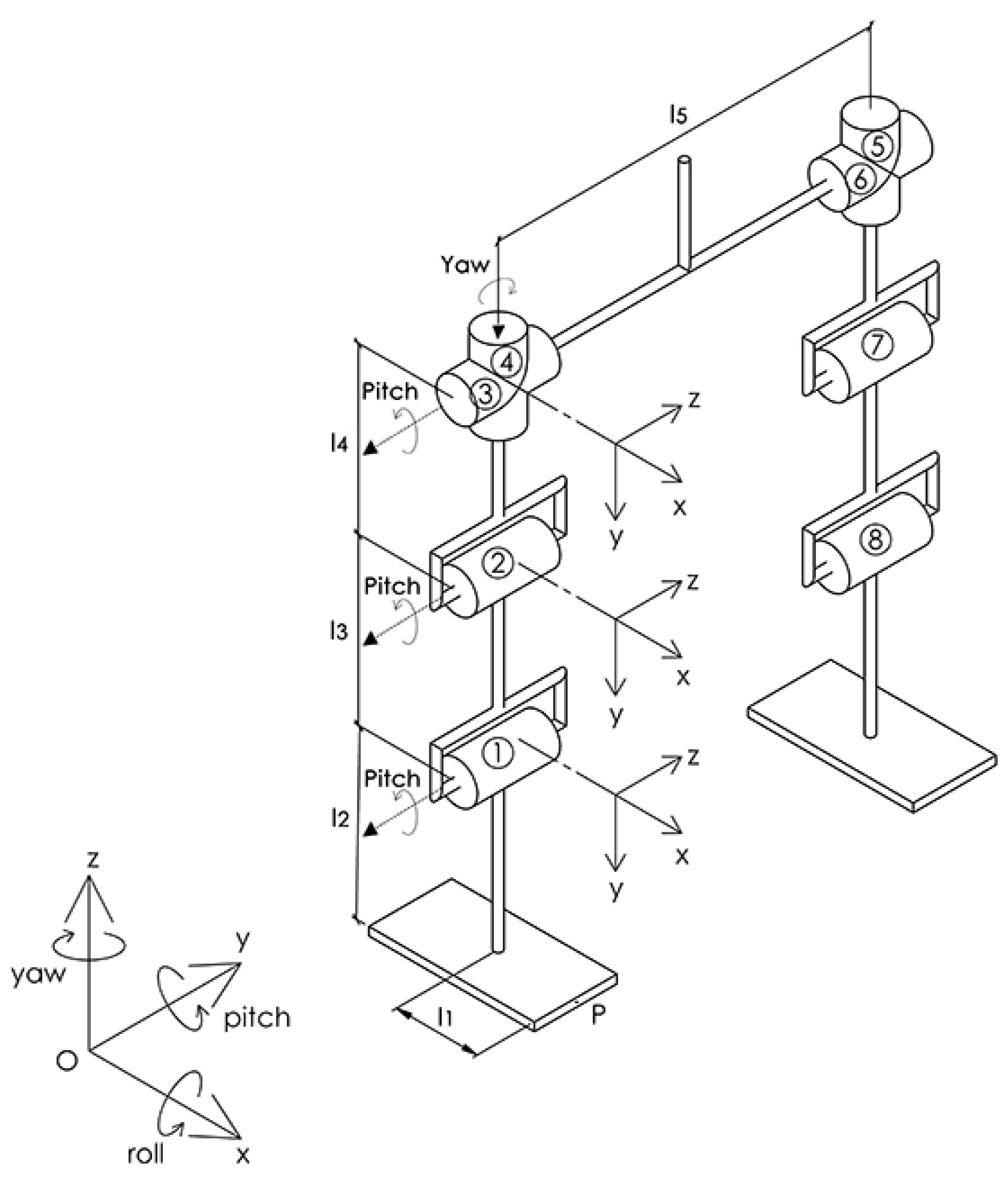
Figure 2.
Flowchart of the proposed algorithm.
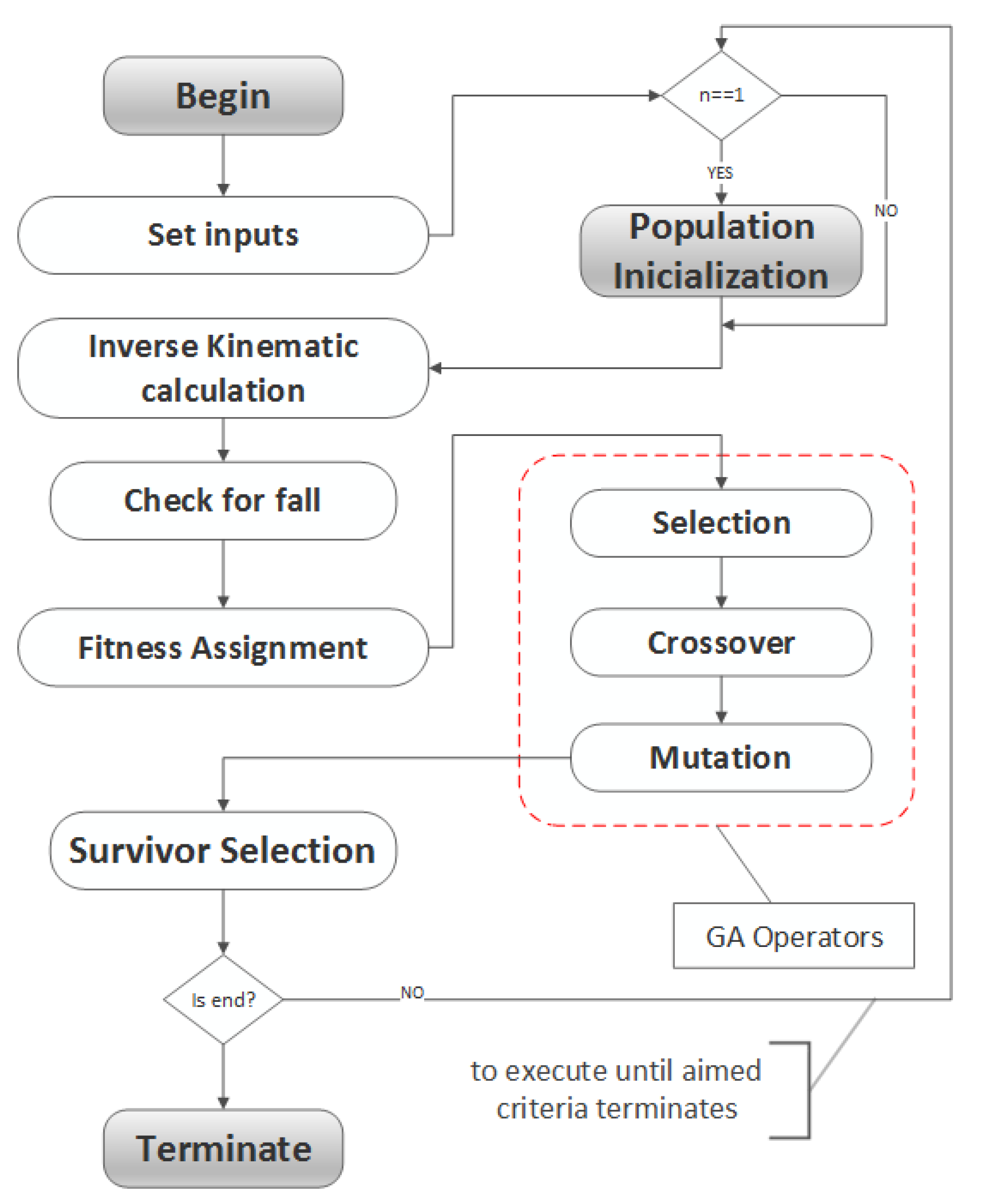
Figure 3.
Chromosome encoding.
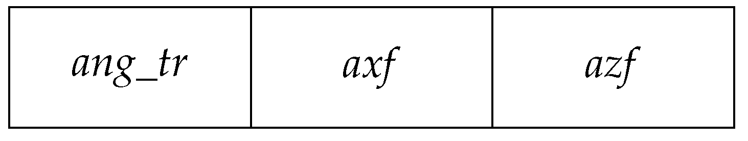
Figure 5.
The graphical interface of the simulator: The orange rectangle indicates the robot objects. The red rectangle shows the Side, Front, Top and Isometric views. The green rectangle makes the variable information available after the simulator runs, and the blue rectangle shows the command window.

Figure 6.
Each block shows the robot in the side, front, top and isometric views. The sequence illustrates a complete gait cycle with optimized walking parameters.
Figure 6.
Each block shows the robot in the side, front, top and isometric views. The sequence illustrates a complete gait cycle with optimized walking parameters.
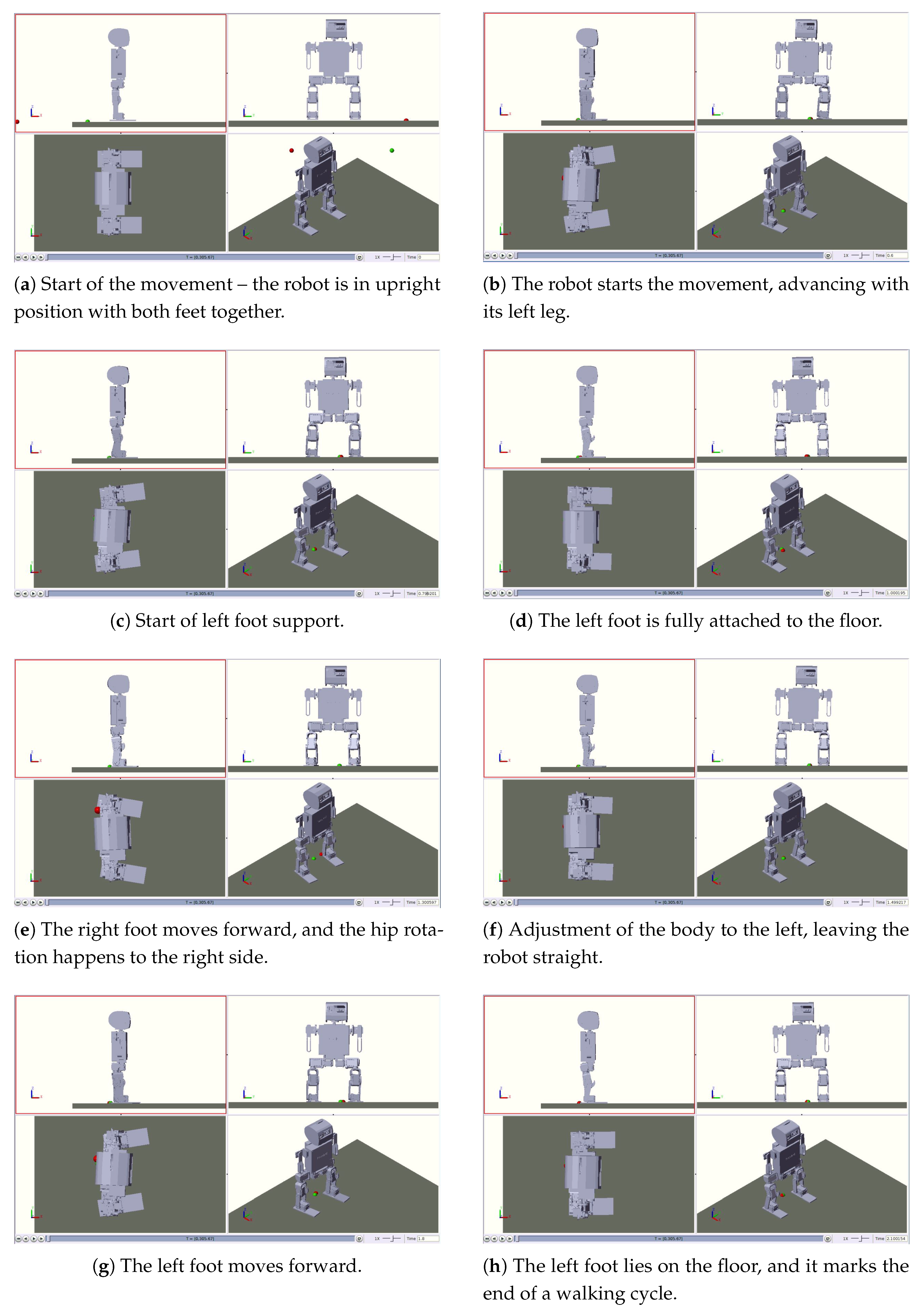
Figure 7.
Convergence of (a) fitness and (b) lateral deviation over 500 generations.
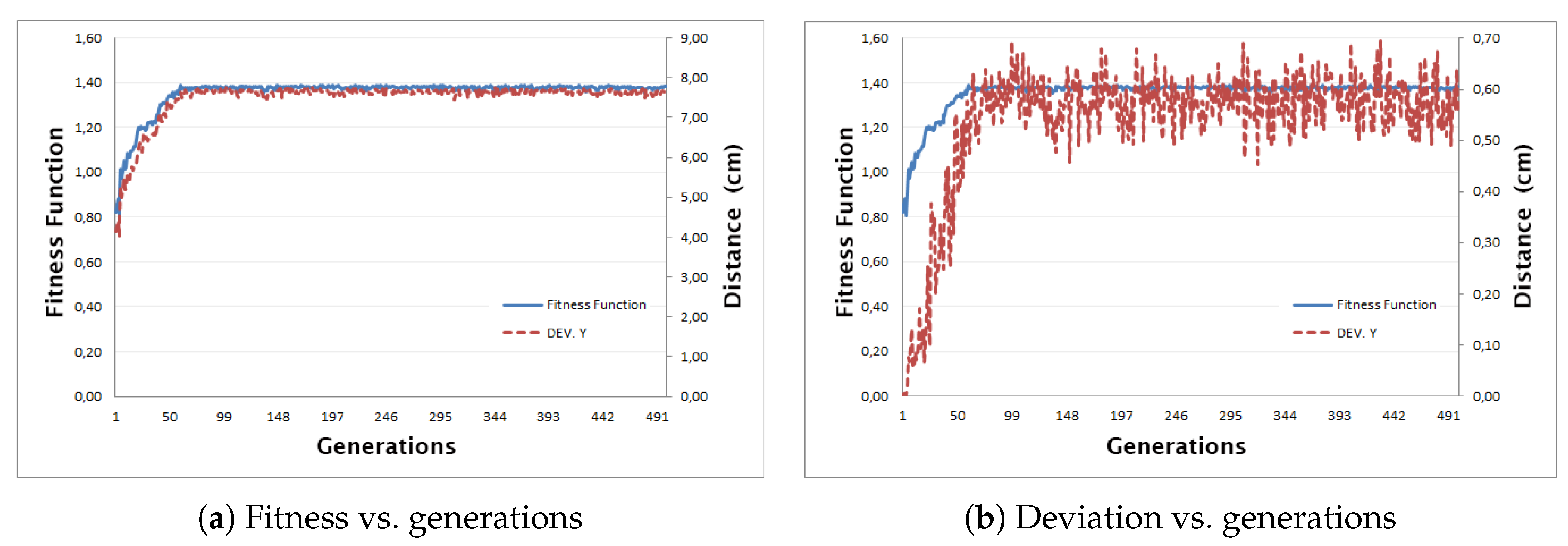
Figure 8.
50-generation run (see Table 3).
Figure 8.
50-generation run (see Table 3).
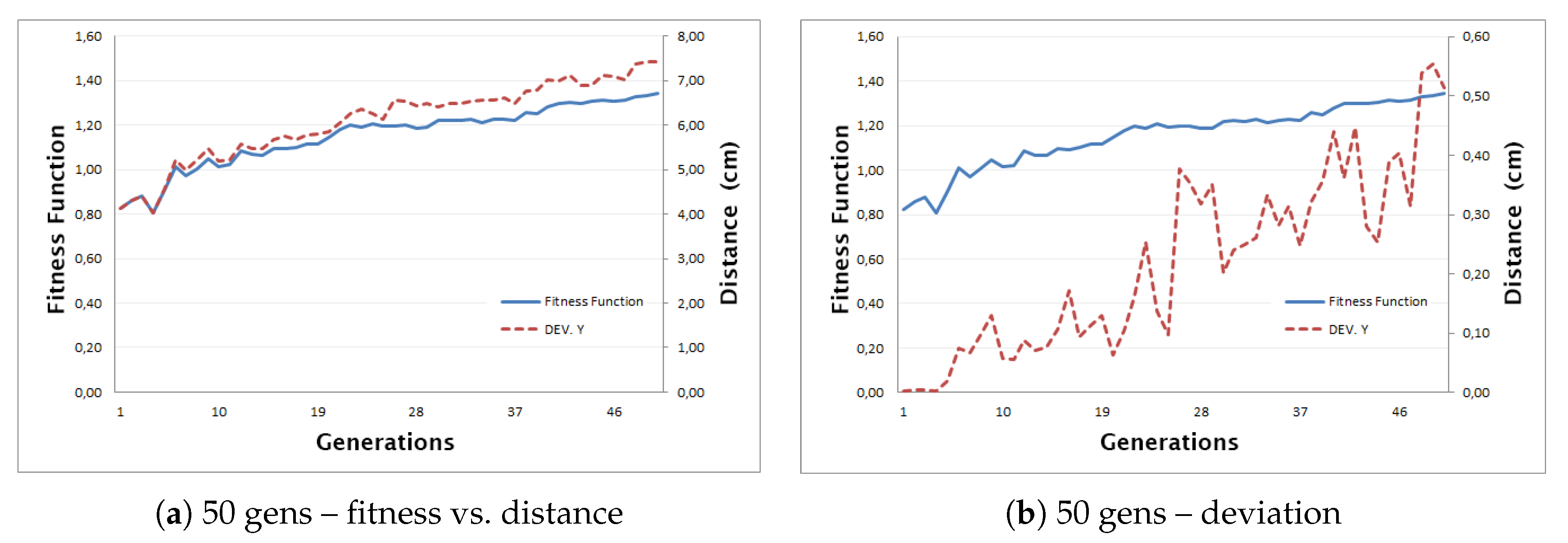
Figure 9.
100-generation run (see Table 3).
Figure 9.
100-generation run (see Table 3).
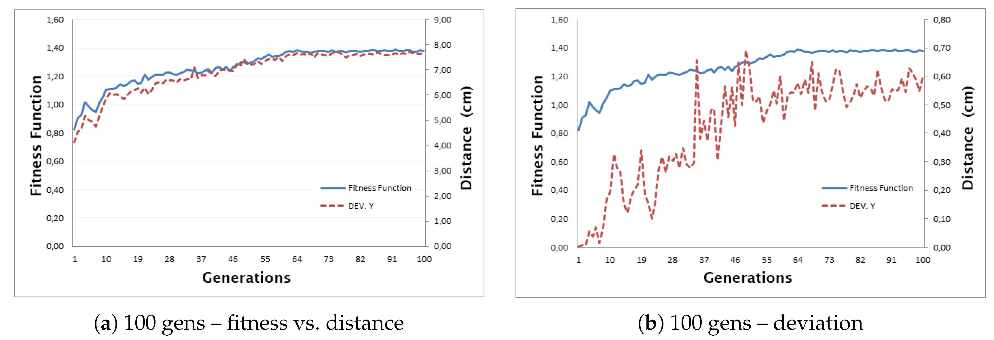
Figure 10.
Optimized joint angle profiles and CoM trajectory over eight gait cycles.

Figure 11.
Key frames from physical-robot gait demonstration (start: a–c; middle: d–f; end: g–i).
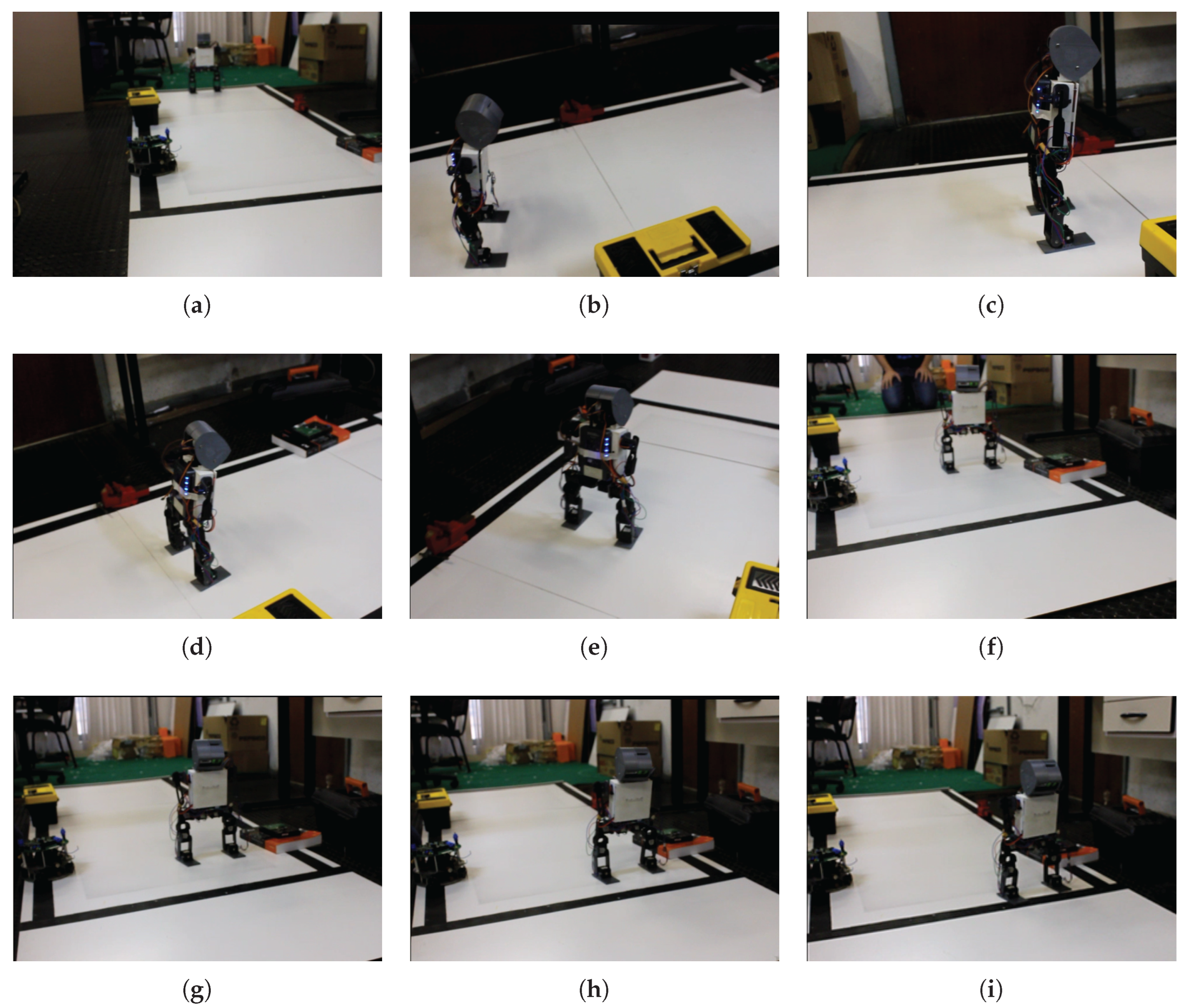

Table 1.
Screw Parameters
| Screw Parameters | Distances | |||||||
|---|---|---|---|---|---|---|---|---|
| 1 | 0 | -1 | 0 | 0 | ||||
| 2 | 0 | -1 | 0 | 0 | ||||
| 3 | 0 | -1 | 0 | 0 | ||||
| 4 | 0 | 0 | -1 | 0 | ||||
| 5 | 0 | 0 | -1 | |||||
| 6 | 0 | -1 | 0 | |||||
| 7 | 0 | -1 | 0 | |||||
| 8 | 0 | -1 | 0 | |||||
Table 2.
Initial population (Gen stands for Generations.)
| Gen. | Gen. | ||||||
|---|---|---|---|---|---|---|---|
| 1 | 5 | 15 | 20 | 6 | 6 | 20 | 30 |
| 2 | 2 | 50 | 50 | 7 | 8 | 80 | 90 |
| 3 | 4 | 25 | 60 | 8 | 12 | 20 | 30 |
| 4 | 1 | 40 | 60 | 9 | 10 | 40 | 25 |
| 5 | 10 | 70 | 50 | 10 | 15 | 60 | 80 |
Table 3.
Summary of fitness–distance and fitness–deviation correlations
| Generations | ||
|---|---|---|
| 50 | 0.8912 | 0.6767 |
| 100 | 0.7444 | 0.6300 |
| 500 | 0.7379 | 0.5736 |
Disclaimer/Publisher’s Note: The statements, opinions and data contained in all publications are solely those of the individual author(s) and contributor(s) and not of MDPI and/or the editor(s). MDPI and/or the editor(s) disclaim responsibility for any injury to people or property resulting from any ideas, methods, instructions or products referred to in the content. |
© 2025 by the authors. Licensee MDPI, Basel, Switzerland. This article is an open access article distributed under the terms and conditions of the Creative Commons Attribution (CC BY) license (http://creativecommons.org/licenses/by/4.0/).
Copyright: This open access article is published under a Creative Commons CC BY 4.0 license, which permit the free download, distribution, and reuse, provided that the author and preprint are cited in any reuse.


