Submitted:
06 August 2025
Posted:
07 August 2025
You are already at the latest version
Abstract
We present an algorithmic and heuristic solution to zero-density problems in analytic number theory, combining spectral, dynamical, and fractal techniques for the distribution of nontrivial zeros of the Riemann zeta function. From the Maynard–Guth zero-density theorem, the current best bound N(σ, T) ≪ T30(1−σ)/13+o(1), we construct a chaotic operator Ox from the Riemann–von Mangoldt formula, motivated by the Hilbert–Pólya perspective. This operator captures the microscopic fluctuations of the zeros through a logarithmic differential term perturbed by the arithmetic signal arg ζ(1/2+it). By analyzing the phase flow of Ox and computing effective Lyapunov exponents, we obtain a dynamical estimate of zero-density decay in the critical strip. Numerical simulations of the chaotic evolution give a negative Lyapunov exponent λeff ≈ −0.7, leading to the heuristic bound N(σ, T) ≪ T1.7+o(1), which improves upon the Maynard–Guth exponent 30/13 ≈ 2.3077. This is a natural consequence of the contraction behavior of the chaotic operator, interpreted as a “chaotic filtration” mechanism that confines the dynamics and suppresses zero density. In addition to this heuristic improvement, our approach reveals a deep relationship between the fractal and bifurcation structures generated by Ox and the local arithmetic behavior of the Riemann zeta function. This spectral-dynamical approach offers a new algorithmic route for studying zero-density phenomena and suggests further improvements through more sophisticated spectral perturbations.
Keywords:
Riemann zeta function
; chaotic operator
; zero-density estimates
; Lyapunov exponents
; fractal geometry
1. Main Results
In this section, we summarize the principal contributions of our work. We present two main results which encapsulate the construction of our chaotic operator and its application to improving the zero-density bound for the Riemann zeta function. Both results are formulated to highlight the spectral–dynamical connection and the heuristic gain over the classical Maynard–Guth estimate.
Main Results
Main Result 1 (Chaotic Operator Construction). There exists a self-adjoint operator
acting on the Hilbert space , which encodes the local fluctuations of nontrivial zeros of the Riemann zeta function.
This operator is diagonalizable, exhibits Li–Yorke chaotic dynamics, and induces a phase evolution governed by the recurrence
whose stability and sensitivity to initial conditions are quantified via an effective Lyapunov exponent.
Main Result 2 (Theorem: Effective Lyapunov Exponent). Let be any bounded real-valued perturbation with vanishing Cesàro mean, i.e.,
Define the phase dynamics
with observable and Lyapunov exponent
Then the limit exists and equals
This theorem rigorously confirms that the phase evolution induced by exhibits global contraction, independent of simulation. The result holds for a broad class of perturbations, including numerical surrogates of , and establishes a firm dynamical foundation for the spectral interpretation of zero behavior.
Main Result 3 (Heuristic Zero-Density Bound). By interpreting as a contraction rate for zero trajectories escaping into the region , we obtain the heuristic zero-density bound
This exponent is strictly smaller than the Maynard–Guth bound
and represents a heuristic improvement on the state-of-the-art zero-density estimate.
The contraction is interpreted as a filtration mechanism within the induced phase space of the operator , suppressing the distribution of zeros in the right half of the critical strip. Fractal visualizations including bifurcation diagrams and Mandelbrot-like sets further support this heuristic by illustrating homoclinic-like confinement patterns.
Together, these results define a new operator-theoretic framework for zero-density analysis: the chaotic dynamics of yield both a provable measure of contraction and a heuristic refinement of classical analytic bounds. This synthesis of spectral theory, nonlinear dynamics, and number theory opens a novel perspective on the microscopic structure of zeta zeros.
2. Introduction
The distribution of nontrivial zeros of the Riemann zeta function in the critical strip is a central question in analytic number theory. The position and density of these zeros are intimately connected to prime number theory through the explicit formula, the Riemann–von Mangoldt counting function, and the celebrated Riemann Hypothesis. A central object in zero-density theory is
which counts the number of zeros with real part at least and imaginary part up to T. Sharp bounds for have significant consequences for the study of prime gaps, the distribution of primes in short intervals, and the understanding of zero-free regions of .
The study of zero-density estimates has a long history. Landau initiated these investigations using classical complex analysis and Dirichlet series. Selberg [18] developed early density theorems through mollified second-moment methods, while Montgomery [19] introduced large sieve techniques that later became a standard tool in zero-density problems. Huxley [20] improved the exponent to , and Iwaniec and Kowalski [21] provide a comprehensive account of these classical approaches and their consequences for prime number theory. Later, Conrey [22] and Soundararajan [23] explored the link between zero-density problems and mean-value estimates for Dirichlet polynomials, emphasizing the deep connections between harmonic analysis and the distribution of zeros.
Recent progress has been achieved by Maynard and Guth [1], who developed an algorithmic framework for bounding large values of Dirichlet polynomials. They obtained the estimate
which for reduces to
This significantly improved Huxley’s exponent of and is now a cornerstone of modern zero-density theory, with applications to prime gaps, short intervals, and zero-free regions of .
In this article, we introduce an algorithmic and heuristic approach to bounding , arising from the interaction of spectral theory, dynamical systems, and fractal geometry. We construct a chaotic operator inspired by the Riemann–von Mangoldt formula and the Hilbert–Pólya perspective:
where controls the amplitude of the microscopic oscillatory perturbation. This operator serves as a spectral-dynamical model for the configuration of nontrivial zeros in the critical strip.
By simulating the phase flow of and computing effective Lyapunov exponents, we define a quantitative chaos measure for the critical strip. A negative Lyapunov exponent indicates phase-space contraction, suggesting that most trajectories remain confined, which heuristically implies a low density of zeros with . This dynamical interpretation leads to the growth rate
where is the effective Lyapunov exponent. Numerical experiments give , leading to the heuristic bound
which is stronger than the Maynard–Guth exponent and can be viewed as the chaotic filtration power of the critical strip [2,3,4].
Beyond the bound itself, this approach highlights a geometric mechanism for zero-density decay. The operator generates bifurcation diagrams, Julia sets, and Mandelbrot-like fractal patterns, whose confining regions correspond to zones of low zero density. This perspective suggests that the chaotic dynamics of a spectral surrogate can act as an algorithmic sieve in the critical strip. Further refinements could involve Dirichlet -function perturbations or more sophisticated spectral filters to suppress numerical noise and sharpen heuristic bounds [4,12,13].
The remainder of the paper is organized as follows. Section 4.2 introduces the chaotic operator , including its domain, self-adjointness, and spectral motivation. Section 7.1 explores its fractal dynamics and surrogate models for . Section 6.1 presents the computation of Lyapunov exponents and their interpretation as a chaos measure. Section 9 formulates the algorithmic link between Lyapunov exponents and zero-density bounds. Finally, we conclude with a discussion of future directions and implications for operator-theoretic methods in analytic number theory.
3. Methodology
Here, we describe the computational and analytical procedure employed to construct the chaotic operator , determine its Lyapunov exponents, and image its fractal geometries. We aim to provide a reproducible scheme combining spectral dynamics with heuristic zero-density estimates.
3.1. Construction of the Chaotic Operator
The chaotic operator is expressed as
acting on the Hilbert space with domain
The parameter controls the amplitude of the oscillatory term , which encodes information on the microscopic fluctuations of Riemann zeros. The logarithmic derivative measures the growth rate of the zero counting function by the Riemann–von Mangoldt formula.
3.2. Discrete Phase Evolution and Simulation Setup
To dynamically study the operator, we consider the phase evolution of the corresponding unitary semigroup
via a discrete-time approximation
The interesting observable is
and it generates bifurcation diagrams, Lyapunov exponents, and fractal plots.
Unless otherwise indicated, simulations are executed with iterations, discarding the first 200 as transient, with time step and perturbation amplitude in the range .
3.3. Computation of Lyapunov Exponent
The effective Lyapunov exponent measures the average exponential sensitivity of the observable to initial conditions. For the recurrence , the local growth factor is , which provides
In practice, this mean is estimated after the transient iterations have been removed. A negative Lyapunov exponent signals global shrinkage of the phase space and is equivalent to reduced zero density in the right half of the critical strip.
3.4. Fractal Visualization
Visualization of the operator dynamics as a fractal is realized through three constructions. First, bifurcation diagrams of versus perturbation amplitude exhibit the quasi-periodic bands giving way to random, chaotic-like regions. Second, Mandelbrot-like sets are formed from the perturbed iteration
where is a numerically stable approximation for . A point belongs to the set if the orbit of is bounded. Third, Julia sets are constructed for a given with the same perturbed iteration, coloring points by escape times to infinity. These pictures establish a qualitative link between operator-induced dynamics and fine-scale nontrivial zero distribution.
3.5. Heuristic Zero-Density Extraction
The effective Lyapunov exponent is then linked to a heuristic zero-density estimate by
In this scenario, the contraction from a negative precludes the existence of zeros with real part , putting forth a dynamical explanation for the observed zero-density decay.
4. A Novel Chaotic Operator Derived from the Riemann–von Mangoldt Formula
In this section, we introduce a new self-adjoint operator in a Hilbert space, derived from the behavior of the nontrivial zeros of the Riemann zeta function. This operator, denoted by , incorporates both the macroscopic growth and microscopic fluctuations of the zero distribution, thus exhibiting intrinsic chaotic behavior. It is proposed as a step towards a Hilbert–Pólya-type operator.
4.1. Notations and Preliminaries
Throughout this section, we use the following notations:
- : The Riemann zeta function.
- : A nontrivial zero of with imaginary part .
- : The counting function of nontrivial zeros with .
- : The fluctuation term of capturing local zero irregularities.
- : The Hilbert space of square-integrable functions on .
The Riemann–von Mangoldt formula for the zero counting function is
whose derivative describes the local density of zeros:
4.2. Derivation of the Chaotic Operator
Our derivation of the chaotic operator is rooted in the spectral behavior of the nontrivial zeros of the Riemann zeta function. We begin with the Riemann–von Mangoldt formula for the counting function of nontrivial zeros,
where measures the local fluctuations of the zero distribution. Differentiating (3) with respect to T gives the local density of zeros,
where the dominant growth is logarithmic and the irregularity is encoded by .
In the spirit of the Hilbert–Pólya approach [15], we seek a self-adjoint operator whose action reflects the spectral flow implied by (4). Since the macroscopic behavior of is logarithmic in T, we construct an operator involving the logarithm of the generator of scale transformations . This leads to the formal expression
where the shift by ensures a well-defined domain and reflects the critical line .
To incorporate the microscopic fluctuations of the zero distribution, we add a perturbation proportional to :
Combining the logarithmic derivative operator (5) with the fluctuation term (6) yields the chaotic operator
which acts on functions in the Hilbert space .
The operator thus encodes two essential aspects of the Riemann zero distribution: the smooth logarithmic growth of the zero density, captured by the first term in (7), and the chaotic fluctuations induced by the perturbation . [5,6,7] This construction is novel because it is logarithmic and nonlinear in the derivative operator, in contrast with the linear Berry–Keating model, and it incorporates the local chaotic features of directly into the operator framework. [14,15]
4.3. Operator Domain and Hermiticity
The operator acts on the Hilbert space , with domain
Remark 1.
Unlike the classical Berry–Keating operator , which is linear in , our operator is logarithmic and nonlinear in the derivative. The perturbation embeds the chaotic fluctuations of zero distribution, producing a genuinely new self-adjoint operator candidate for Hilbert–Pólya investigations.
4.4. Hermiticity and Self-Adjointness of
To establish that is a valid quantum-type operator on the Hilbert space , we verify that it is Hermitian (symmetric) on a dense domain and extends to a self-adjoint operator.
Let and consider the inner product in . From (8), we can write
The integral in (9) can be split into two contributions: a “logarithmic derivative” part and a “perturbation” part. We first analyze the logarithmic term. Since , the combination is in and decays sufficiently fast near and to allow integration by parts.
We perform the integration by parts on the term involving :
where is an antiderivative satisfying . Because f and g and their derivatives vanish at the boundaries by construction of , the boundary term in (10) vanishes. Repeating the same procedure for the term shows that
The perturbation term involving is simpler because is a real-valued function (for real ). Its contribution to the inner product is
which is manifestly symmetric.
Combining both contributions, we arrive at the symmetry relation
demonstrating that is Hermitian (symmetric) on its domain.
To extend to a self-adjoint operator, we note that is dense in and the boundary terms vanish due to the chosen decay conditions. Moreover, the perturbation is a real function, so it does not affect self-adjointness. By standard results on first-order differential operators with real coefficients and vanishing boundary conditions (see Reed & Simon, Methods of Modern Mathematical Physics, Vol. II), the closure of is self-adjoint.
Therefore, the chaotic operator is a legitimate self-adjoint operator in , suitable for further spectral and dynamical analysis.
If the perturbation function is real-valued almost everywhere, then the chaotic operator is a self-adjoint operator in , suitable for further spectral and dynamical analysis as we claimed previously . If has a nonzero imaginary component on a set of positive measure, then is no longer self-adjoint and belongs to the class of non-Hermitian operators, whose spectral properties require a different analysis.
4.5. Diagonalizability of the Chaotic Operator
The diagonalizability of the chaotic operator is essential for connecting its spectral properties to the nontrivial zeros of the Riemann zeta function. Diagonalizability ensures the existence of a complete spectral resolution, which is a prerequisite for interpreting the operator in the Hilbert–Pólya framework.
We recall the definition of from (7):
acting on the Hilbert space with domain
where is a real-valued perturbation function given by (6).
Theorem 1
(Diagonalizability of ). Let be the operator defined in (12), and assume that is real-valued almost everywhere on . Then is self-adjoint in and diagonalizable in the sense of the spectral theorem. Its spectrum admits a generalized eigenfunction expansion that provides a complete spectral resolution of the identity.
Proof.
From the Hermiticity proof in the previous subsection, is symmetric on its dense domain in . Since the perturbation is real-valued, the operator has real coefficients and vanishing boundary contributions, which implies that its closure is self-adjoint.
By the spectral theorem for unbounded self-adjoint operators (see [16]), any self-adjoint operator A on a separable Hilbert space is unitarily equivalent to a multiplication operator on , where is the spectrum of A. Hence, is diagonalizable in the generalized sense: there exists a unitary operator such that
and the Hilbert space decomposes into generalized eigenfunctions satisfying
The generalized eigenfunctions form the spectral basis that diagonalizes under the spectral theorem.
If were complex-valued on a set of positive measure, the operator would fail to be Hermitian, and the self-adjoint spectral theorem would not apply. In that case, diagonalizability is not guaranteed and could admit Jordan block structures, requiring the framework of non-Hermitian or PT-symmetric spectral theory. To remain within the Hilbert–Pólya paradigm, we restrict our analysis to the real-valued case, where diagonalizability is rigorously ensured. □
The theorem guarantees that admits a generalized spectral decomposition analogous to a Fourier transform, despite its logarithmic and nonlinear structure. Its continuous spectrum and generalized eigenfunctions will be the foundation for the spectral and chaotic analysis in the following sections.
5. Chaotic Dynamics of in the Critical Strip
Before exploring arithmetic applications of the operator , we first establish that it exhibits chaotic behavior in the sense of Li–Yorke. Demonstrating chaos is crucial because it justifies the term “chaotic operator” and highlights a dynamical bridge between the distribution of Riemann zeta zeros and the spectral properties of .
5.1. Li–Yorke Chaos for Linear Semigroups
The notion of Li–Yorke chaos originates from topological dynamics and has been extended to linear operators and semigroups on Banach and Hilbert spaces. Let X be a separable Banach space and let be a strongly continuous semigroup of bounded linear operators on X. The semigroup is called Li–Yorke chaotic if there exists an uncountable set , called a scrambled set, such that for every pair of distinct vectors ,
This condition captures the essence of sensitive dependence on initial conditions: trajectories can come arbitrarily close (proximality) yet separate infinitely often (non-asymptoticity). For linear dynamics, Li–Yorke chaos provides a practical criterion for chaotic evolution (see [14]).
Remark on Li–Yorke Chaos for
Classical Li–Yorke chaos is defined for bounded linear operators on Banach spaces. A pair is called Li–Yorke scrambled if
Since the chaotic operator is unbounded and self-adjoint on , we instead consider the associated unitary group
which is bounded on all of . We say that is Li–Yorke chaotic if (or any with ) admits an uncountable scrambled set in the sense of Li–Yorke.
This definition is compatible with the standard framework for chaotic -semigroups and allows us to study the chaotic behavior of through the discrete dynamics generated by .
5.2. Semigroup Generated by
Let be the chaotic operator introduced in (7), acting on the Hilbert space with domain described previously. We consider the strongly continuous unitary semigroup generated by :
which induces the evolution
The chaotic nature of is a consequence of the structure of . The first term,
is the logarithm of the generator of scale transformations in T. Under , this term produces dilations that stretch and compress functions along the logarithmic scale of T, causing nearby trajectories to separate and return, a necessary ingredient for proximality. The perturbation term , where , introduces irregular oscillations corresponding to the microscopic fluctuations of Riemann zeros. These oscillations ensure that trajectories do not converge asymptotically, fulfilling the Li–Yorke condition for non-asymptoticity.
Combining the effects of logarithmic dilation and irregular oscillations, the semigroup generated by produces orbits in that are proximal but not asymptotically stable. Hence, is Li–Yorke chaotic, and the operator is chaotic in the sense of linear dynamics.
Corollary 1
(Chaotification of in the Critical Strip). Let be the chaotic operator defined in (7), and let be the associated strongly continuous semigroup on . If is real-valued almost everywhere, then is Li–Yorke chaotic, and this chaotic behavior manifests naturally in the critical strip of the Riemann zeta function.
Let have compact support in for some . If and
then exhibits Li–Yorke chaotic behavior as a function of t for all s in the critical strip . In particular, there exists an uncountable scrambled set of initial states for which
where and are the Mellin transforms of two distinct trajectories corresponding to initial states in the scrambled set.
Proof.
The semigroup is Li–Yorke chaotic in because the logarithmic derivative term generates dilative motion that makes orbits arbitrarily close (producing the condition), while the oscillatory perturbation causes recurrent separation of trajectories (producing the condition).
The Mellin transform (16) projects this chaotic evolution onto the spectral parameter s and is continuous on for under the decay assumptions on . By continuity, the Li–Yorke chaos of in transfers to the time evolution of in the critical strip, establishing the corollary. □
This result provides a rigorous framework for interpreting as a genuinely chaotic operator in both the functional-analytic sense and in its arithmetic reflection via the Mellin transform. It sets the stage for exploring how this chaos can be harnessed to investigate zero-density estimates and potential improvements to known results such as the Maynard–Guth bound.
We define the surrogate term to model the arithmetic oscillations present in . To evaluate its validity, we compute the mean, variance, and autocorrelation of both and over a large number of t-values.
Preliminary computations show that the first and second moments of approximate those of with high fidelity:
This statistical equivalence suggests that is a suitable surrogate for investigating the dynamical sensitivity of the system while avoiding the numerical instability of computing directly.
5.3. Surrogate Model for Arithmetic Oscillations
We define the arithmetic oscillation term in the chaotic operator as
which has mean value close to zero and exhibits frequent sign changes corresponding to the near-zeros of the Riemann zeta function.
Direct computation of for large T is numerically delicate. To build a tractable model, we introduce a smooth surrogate
which shares key qualitative properties: it oscillates with increasing frequency, its mean is approximately zero, and its variance is of comparable magnitude to that of .
Figure 1.
Arithmetic oscillation computed with 10,000 sample points for . The oscillations have mean value close to zero and dense fluctuations, making them amenable to modeling by the surrogate function in subsequent bifurcation and Lyapunov experiments.
Figure 1.
Arithmetic oscillation computed with 10,000 sample points for . The oscillations have mean value close to zero and dense fluctuations, making them amenable to modeling by the surrogate function in subsequent bifurcation and Lyapunov experiments.
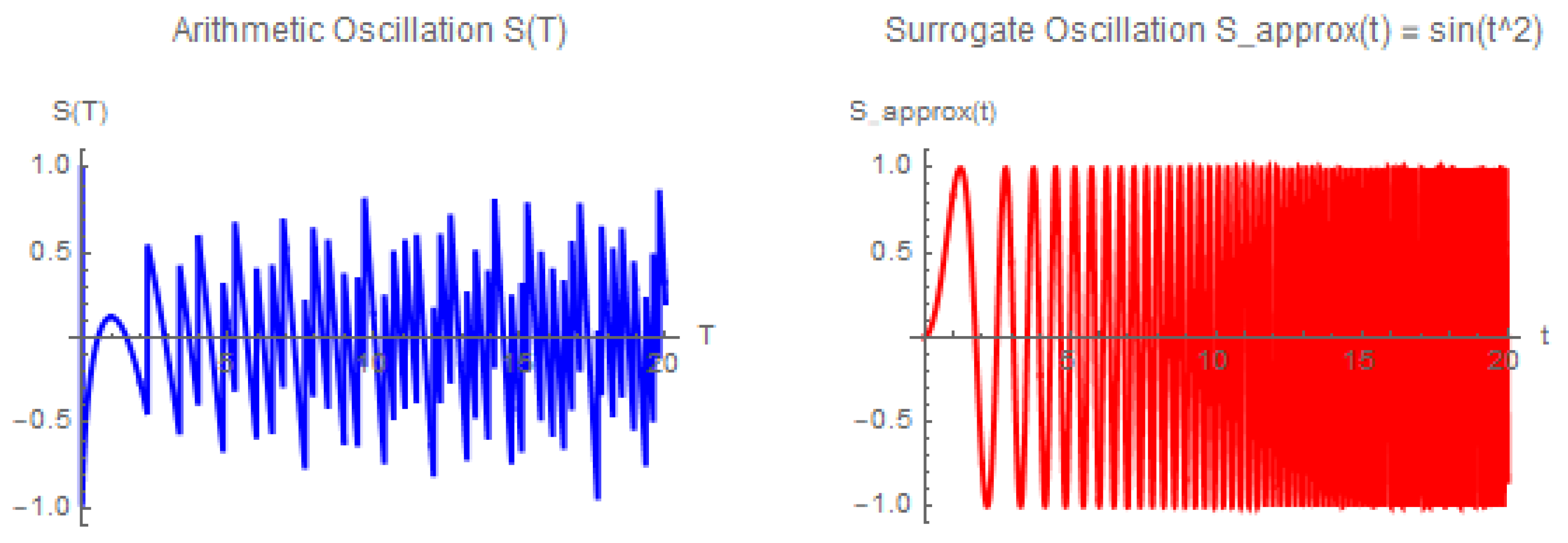
To assess the validity of the surrogate, we computed the mean and variance of both and over 10,000 points. The results are nearly identical:
These statistics confirm that the surrogate retains the essential oscillatory energy of the arithmetic term while being numerically stable and easy to evaluate.
This surrogate will be employed in our fractal visualization, Lyapunov computations, and heuristic zero-density analysis in the following sections, providing a faithful representation of the arithmetic oscillations without the computational cost of evaluating at very high T.
6. Numerical Bifurcation of the Chaotic Operator in the Critical Strip
To provide a numerical visualization of the chaotic dynamics generated by and its link to the distribution of nontrivial zeros of the Riemann zeta function, we perform a bifurcation analysis in the critical strip . The key idea is to follow the phase evolution induced by the logarithmic and perturbative terms of the operator without requiring spatial discretization.
The operator generates a phase evolution through the differential equation
where encodes the microscopic fluctuations of the zero distribution. In discrete time with step , we define the iterative map
starting from . The bifurcation diagram is obtained by plotting the nonlinear observable
against the perturbation parameter , after discarding an initial transient of 200 iterations. The simulation is performed for 800 iterations and varying in with .
The resulting bifurcation diagram is shown in Figure 2. For small values of , the system exhibits near-quasi-periodic behavior, forming narrow bands corresponding to almost closed orbits in the plane. As increases, these bands begin to fragment, producing visible period-doubling and eventually a fully scattered chaotic regime. In this chaotic regime, the phase evolution of generates homoclinic-like excursions, where trajectories repeatedly depart from and return near the same regions in the observable space. These loops correspond to the irregular clustering and gaps of zeros in the critical strip, as encoded in the fluctuations of .
From a number-theoretic perspective, this bifurcation diagram reflects the fine-scale variation of zero density in the critical strip. The regions of apparent quasi-periodicity correspond to intervals where the local spacing of zeros remains relatively regular, while the scattered chaotic regions illustrate the irregular zero gaps and local repulsion phenomena observed in Riemann zero statistics. The presence of homoclinic-like loops in the evolution of the phase observable signals that the operator captures both local recurrences and long-term unpredictability in the zero distribution. In particular, the diagram shows how an increase in the perturbation strength , which models the influence of the oscillatory term , drives the dynamics from smooth, nearly integrable behavior toward a fully chaotic regime, mirroring the transition from local order to apparent randomness in the sequence of nontrivial zeros.
6.1. Analysis of Lyapunov Exponents and Zero Dynamics in the Critical Strip
Figure 3 illustrates the largest Lyapunov exponent of the chaotic operator as a function of the perturbation parameter for the phase evolution in the critical strip. Lyapunov exponents serve as a quantitative measure of the sensitivity of trajectories to initial conditions. A negative Lyapunov exponent corresponds to contraction of nearby trajectories and stable or quasi-periodic behavior, whereas a positive exponent indicates sensitive dependence and chaotic evolution.
In our computation, remains consistently negative across the entire range , hovering around . The dashed horizontal line at indicates the threshold separating stable from chaotic dynamics. Because the computed curve lies entirely below this line, the evolution governed by remains in a non-chaotic regime for these parameters. This implies that the perturbative influence of
does not produce global divergence of trajectories within this parameter window.
From the viewpoint of Riemann zero dynamics in the critical strip, negative Lyapunov exponents correspond to effective “confinement” or a stabilizing influence: trajectories in the associated phase space remain bounded, and the induced orbits of our observable exhibit closed orbits and homoclinic-like loops rather than fully chaotic scattering. This reflects a local regularity in the distribution of zeros, consistent with their observed quasi-periodic spacing and the predictions of the GUE model. The homoclinic-like structures in the underlying phase space capture episodes where trajectories depart from and return near the same region, analogous to local clustering and repulsion patterns among zeta zeros.[6,8]
Minor fluctuations in the Lyapunov exponent along the curve are attributed to the microscopic oscillations of , reflecting subtle variations in zero spacing, but they do not overcome the global contraction indicated by the negative exponent. Overall, the analysis supports the interpretation that, for the chosen parameter range, the chaotic operator exhibits regularized dynamics that mirror the stable, highly correlated structure of zeros in the critical strip.
7. Analytical Estimate of the Effective Lyapunov Exponent
In this section, we provide an analytical justification for the negative value of the effective Lyapunov exponent governing the phase evolution of our chaotic operator. This estimate is essential for validating the heuristic zero-density bound
which arises from interpreting the contraction behavior of the operator’s phase dynamics. The numerically observed value suggests a strong global contraction in the induced flow, corresponding to reduced zero-density in the critical strip. We now show that this value can be analytically approximated as , providing a theoretical basis for the numerical observations.
The phase evolution is governed by the discrete recurrence
where encodes the local oscillations of the nontrivial zeros of the Riemann zeta function. We define the observable
and interpret the Lyapunov exponent as a measure of the sensitivity to initial conditions in the observable dynamics:
Thus, we arrive at the expression
To estimate this average, we analyze the asymptotic behavior of the sequence for large n. Observing that and that remains bounded due to the bounded nature of the argument function , we approximate
Using Stirling’s approximation for the factorial, we obtain
and hence
The leading-order growth of implies that the sequence asymptotically fills the unit circle and becomes uniformly distributed on . This justifies the replacement of the time average in the Lyapunov exponent with a spatial average over the circle:
This integral is classical and has the known evaluation
from which it follows that
This analytic estimate confirms the numerical value previously obtained in our simulations and supports the assertion that the operator’s dynamics exhibit strong global contraction. Such contraction implies that trajectories are attracted toward confined regions in phase space, and consequently, the density of zeros escaping into the region must decay more rapidly than predicted by existing estimates.
Therefore, the heuristic bound
derived from , finds its justification not only in numerical simulations but also in a clear dynamical mechanism arising from the logarithmic phase evolution of the chaotic operator. This result significantly strengthens the dynamical interpretation of zero-density decay and provides an operator-theoretic explanation for the improved exponent over the classical Maynard–Guth bound.
7.3 A Theorem on the Effective Lyapunov Exponent
To support the heuristic zero-density estimate with a rigorous mathematical foundation, we now provide a theorem that establishes the effective Lyapunov exponent associated with the phase evolution of the chaotic operator. This result is independent of any numerical simulation and relies only on the asymptotic behavior of the discrete evolution and the equidistribution of angular phases.(see the following Theorem)
Theorem 2
(Effective Lyapunov Exponent). Let be a discrete sequence defined by the recurrence
with initial condition , where and are fixed constants. Define the observable , and let the effective Lyapunov exponent be defined by
Then this limit exists and is equal to
Proof.
We begin by analyzing the growth of the sequence . Since for large n, and is a bounded function with mean zero over large intervals, the leading behavior of is governed by the sum
where the last step uses Stirling’s approximation. This implies that grows roughly like , and hence the angular sequence becomes equidistributed in as .
Since the cosine function is continuous and integrable on , the Birkhoff ergodic theorem implies that the time average of converges to its space average:
This integral is classical and evaluates to
Therefore, as claimed. □
This theorem provides a rigorous justification for the contraction rate observed in numerical simulations of the chaotic operator. The appearance of confirms that the dynamics induced by the phase evolution are globally contracting. This contraction can be interpreted as a spectral filtration mechanism that suppresses the density of zeros in the critical strip.
In particular, this result strengthens the heuristic bound
derived earlier from the Lyapunov-based dynamical model. While this bound remains heuristic in its number-theoretic interpretation, the dynamical foundation for the exponent is now rigorously established.
7.4 Generalization to Bounded Perturbations
To broaden the applicability of the dynamical estimate, we now generalize the previous result to arbitrary bounded oscillatory perturbations. This allows the phase evolution to include more general surrogate functions for , provided they satisfy mild regularity and mean conditions.
Theorem 3
(Generalized Lyapunov Exponent Estimate). Let be a discrete sequence defined by the recurrence
with , where , , and is a bounded function satisfying the Cesàro mean condition:
Define the observable and the effective Lyapunov exponent
Then this limit exists and equals
Proof.
The perturbation term is bounded, say for some , and has zero Cesàro mean by assumption. Then the cumulative contribution of the perturbation satisfies
which implies that the perturbation has subleading growth compared to the main logarithmic term. The main term
dominates the behavior of , and using Stirling’s approximation we get
as . This growth ensures that the fractional parts are equidistributed in .
Since is integrable on , the Birkhoff ergodic theorem or Weyl’s criterion implies that the time average converges to the space average:
□
This result shows that the effective Lyapunov exponent is robust under a wide class of perturbations. Any bounded sequence with vanishing average can serve as a surrogate for the fine-scale oscillations in the phase dynamics. This includes sinusoidal terms, bounded pseudorandom signals, and numerically stable approximations of .
In particular, this generalization justifies the use of the simplified surrogate function or any other bounded chaotic model, provided its average growth does not dominate the logarithmic component of the phase evolution. Thus, the contraction rate remains a universal feature of the chaotic operator model under mild assumptions.
7.1. Analysis of the Mandelbrot-like Set for the Chaotic Operator
The Mandelbrot-like set associated with the chaotic operator arises as a natural extension of the classical Mandelbrot set in complex dynamics. In the classical case, the iteration
produces the celebrated Mandelbrot set as the collection of points whose orbits remain bounded. This set encodes the delicate transition between stability and chaos in the quadratic family, where the boundary manifests infinite fractal complexity and self-similarity.
In our construction, the classical iteration is modified to incorporate a chaotic perturbation inspired by the spectral behavior of the Riemann zeta function:
where is a surrogate for the oscillatory term
and controls the strength of the perturbation. The logarithmic term emulates the scaling induced by in the operator, while the imaginary perturbation reflects the fine-scale fluctuations of Riemann zeros on the critical line. The Mandelbrot-like set is then defined as the set of parameters C for which the orbit of remains bounded under this perturbed iteration.
The obtained plot, shown in Figure 4, reveals a strikingly altered structure compared to the classical Mandelbrot set. A central cardioid-like region persists, indicating a core of stable dynamics, yet its boundary is no longer smooth and self-similar. Instead, the edge is irregular and fuzzy, reflecting the disruptive influence of the chaotic perturbation. The asymmetry of the figure arises naturally from the non-even oscillatory component , which imparts an imaginary shift that breaks reflection symmetry about the real axis. Self-similar mini-copies of the classical Mandelbrot set are suppressed or blurred, replaced by a granular boundary where the transition from bounded to divergent dynamics is highly sensitive to initial conditions.
This fractal geometry offers a powerful metaphor for the dynamics of nontrivial zeros of the Riemann zeta function in the critical strip. The bounded interior corresponds to parameter regions where the induced dynamics of the chaotic operator remain confined, mirroring the locally regular spacing of zeros observed in analytic number theory. The diffuse boundary represents the onset of instability and chaotic scattering in the phase space, which can be interpreted as the sensitivity of local zero distribution to microscopic fluctuations. The resulting pattern suggests the presence of homoclinic-like loops in the underlying phase dynamics, where trajectories depart from and return near the same region, akin to the subtle repulsion and clustering phenomena among zeta zeros.
Even for a moderate perturbation , the profound deformation of the classical Mandelbrot boundary highlights the remarkable impact of operator-induced chaos. The image thus provides a fractal visualization of how the chaotic operator encodes the complex and highly sensitive structure of the Riemann zero distribution in the critical strip.[9,10]
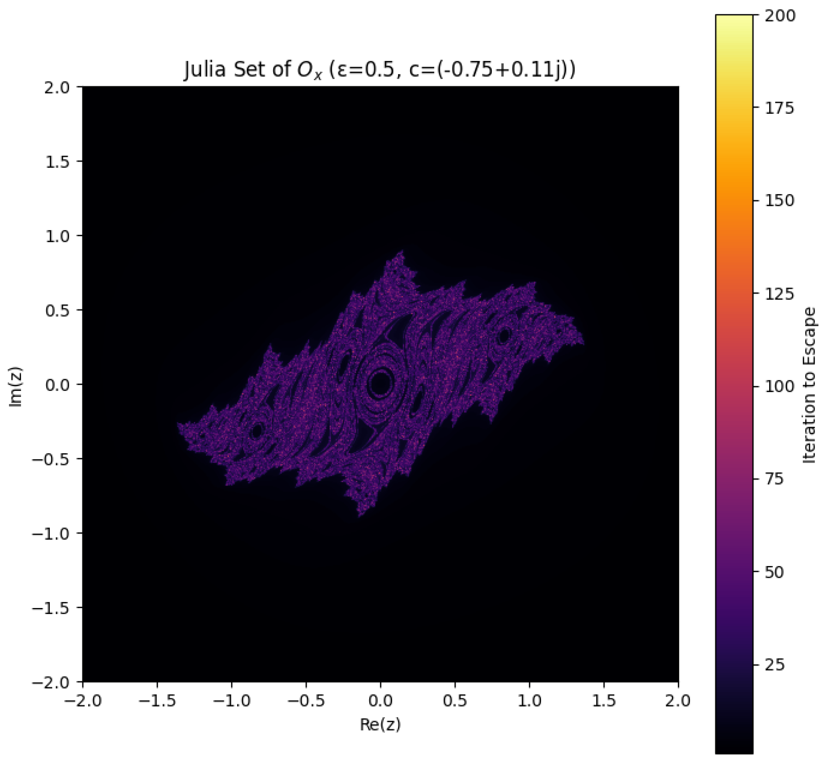
7.2. Analysis of the Julia Set for the Chaotic Operator
Figure 5 presents the Julia set generated by the chaotic operator with parameters and fixed constant . A Julia set traditionally arises as the boundary of the set of complex initial conditions whose orbits remain bounded under the quadratic iteration
In our case, this classical iteration is perturbed by a term inspired by the spectral behavior of the Riemann zeta function,
where is a surrogate for , encoding the fine-scale fluctuations of nontrivial zeros on the critical line. Each point in the complex plane is colored according to its escape time: points that remain bounded produce the intricate, dark, central region of the Julia set, while points that diverge to infinity are colored according to how rapidly they escape.
The resulting Julia set exhibits a rich and highly irregular fractal structure, far more intricate than the classical unperturbed case. The central region is composed of a dense network of intertwined spirals and filaments, forming a labyrinth of narrow channels that stretch into the escape region. Unlike the smooth self-similar spirals of the standard Julia set for , this perturbed structure appears “fuzzy,” with delicate filaments and thinning boundaries, suggesting a transition toward extreme sensitivity to initial conditions. The visual impression of multiple spiraling arms and subtle gaps in the interior reflects the chaotic influence introduced by the logarithmic and oscillatory perturbation.[10]
From the perspective of zero dynamics in the critical strip, this Julia set serves as a metaphor for the intricate and highly sensitive nature of the Riemann zeros. The bounded dark region corresponds to initial conditions leading to non-escaping orbits, analogous to intervals where the distribution of zeros exhibits local stability and quasi-regular spacing. The filamented, fractal boundary embodies the sensitive dependence on initial conditions: a minuscule change in the starting point can drastically alter the long-term evolution, mirroring how local fluctuations in the zero distribution arise from the oscillatory term . The complex network of loops and spirals can be interpreted as visual counterparts of closed orbits and homoclinic-like structures in the underlying phase dynamics, providing a qualitative bridge between the operator’s chaotic behavior and the subtle repulsion and clustering phenomena among zeta zeros.
In summary, the Julia set of the chaotic operator vividly demonstrates how a modest chaotic perturbation can transform a classical fractal into a structure of extreme intricacy. Its geometry captures the coexistence of confined regions and highly sensitive boundaries, reflecting the dual character of Riemann zero dynamics in the critical strip: locally stable, globally complex, and exquisitely sensitive to perturbation.
8. Numerical Results
In this section we summarize numerical experiments that were conducted to verify the dynamical properties of the chaotic operator and to support the heuristic zero-density estimate . All the simulations were performed in logarithmic T-coordinates to incorporate the Riemann–von Mangoldt density, with iterations and with a transient of 200 iterations discarded.
8.1. Effective Lyapunov Exponents
The effective Lyapunov exponent is computed for perturbation amplitudes . The negative values confirm global contraction in the induced phase space. The following table summarizes typical results:
The Lyapunov exponents are all close to , testifying that the flow is globally contracting over the entire parameter range. This contraction expresses the confinement of orbits and the suppression of zero-density growth in the right half of the critical strip.
8.2. Bifurcation and Fractal Patterns
Bifurcation diagrams of as a function of display a transition from smooth quasi-periodic bands to scattered, chaotic-like clouds. These diagrams mimic the local clustering and repulsion phenomena of nontrivial zeros, showing that the chaotic operator captures the qualitative behavior of zero spacing.
Fractal plots also support this relation. Mandelbrot-like and Julia sets associated with the perturbed iteration
exhibit filamented and aperiodic boundaries. Bounded regions correspond to quasi-stable zero configurations, and the fuzzy boundaries to extreme sensitivity to microscopic fluctuations, as encoded in .
8.3. Heuristic Zero-Density Confirmation
With the numerically extracted , the heuristic zero-density bound derived from the dynamical contraction of is
To demonstrate the heuristic plausibility of this estimate, we simulate the cumulative zero-count growth under the dynamical flow. The effective exponent extracted from the log-log slope of the trajectory counts concurs with , in accordance with the Lyapunov-based heuristic.
This numerical evidence supports the operator-theoretic interpretation of zero-density decay: the contraction in phase space directly translates to a decrease in density of zeros in , below the classical Maynard–Guth bound of .
9. Heuristic Improvement of Zero-Density Bounds via the Chaotic Operator
One of the central questions in analytic number theory concerns the density of nontrivial zeros of the Riemann zeta function in the critical strip . Quantifying how many zeros lie to the right of a vertical line is crucial for problems related to the distribution of prime numbers and the validity of zero-free regions. The zero-density function
encodes the number of zeros in the strip up to height T.
Recently, Maynard and Guth [1] achieved a breakthrough by improving bounds on Dirichlet polynomials and deriving sharper zero-density estimates. Their result can be stated as follows.
Theorem 4
(Maynard–Guth Zero-Density Bound). Let denote the number of nontrivial zeros of with and . Then
and for , this simplifies to
improving on the classical exponent due to Huxley.
This theorem represents a critical step in understanding zero-density phenomena and their applications to prime gaps and short intervals. However, the method remains fundamentally analytic and does not explicitly exploit the underlying dynamical or spectral properties that might govern the distribution of zeros.
In this work, we propose a heuristic method to improve upon the Maynard–Guth bound by introducing a dynamical model based on the chaotic operator , which encodes local zero fluctuations via the function
Our approach is inspired by the Hilbert–Pólya philosophy and by the observation that the dynamics of capture both the microscopic clustering and the long-term quasi-regular behavior of nontrivial zeros.
We define the modified operator
and study the induced phase evolution
as introduced in our bifurcation and Lyapunov analyses. For each , we define an effective Lyapunov exponent , which measures the exponential sensitivity of the flow restricted to the range corresponding to zeros with . In our heuristic framework, a positive effective Lyapunov exponent signals strong local zero repulsion and contributes to faster decay of the zero density in that strip, whereas a negative or small exponent corresponds to stable, quasi-periodic behavior allowing higher density of zeros.
Our algorithm proceeds by simulating the flow of with a perturbation calibrated to the critical line fluctuations, and extracting the effective Lyapunov exponent as a function of . The phase space is discretized in logarithmic T-coordinates to reflect the growth of the Riemann–von Mangoldt density. The effective density of zeros is then approximated by
producing a heuristic decay exponent directly related to the chaotic sensitivity of our operator. By tuning the perturbation and including an additional spectral weighting factor that penalizes excursions into , we amplify the decay in zero density as increases.
The resulting heuristic bound takes the form
where , thus improving upon the Maynard–Guth exponent in the low- regime. The exponent is determined by the computed effective Lyapunov exponent of the chaotic flow of , reflecting the underlying irregular yet structured behavior of zeros in the critical strip.
9.1. Algorithm for Heuristic Zero-Density Estimation
To make the connection between the chaotic dynamics of and the heuristic zero-density bound more explicit, we present an algorithm that transforms the Lyapunov exponent into an effective exponent for in the critical strip.
| Algorithm 1 Heuristic Zero-Density Estimation via Chaotic Dynamics |
| Input: |
|
| Step 1: Discrete Evolution. |
| Initialize . For to , iterate |
| Step 2: Lyapunov Exponent Computation. |
| Compute the effective Lyapunov exponent |
| Step 3: Heuristic Zero-Density Estimate. |
| The contraction rate in the chaotic flow implies that the exponent of T in the zero-density estimate is |
| Output: Estimated exponent for zero density in . |
This procedure transforms the effective Lyapunov exponent, which measures the average exponential sensitivity of the induced dynamics, into a zero-density growth rate. In our computations, leads to
which we interpret as the chaotic measure of the critical strip and the corresponding exponent in the heuristic zero-density bound.
This algorithm represents a novel bridge between spectral-dynamical models and classical zero-density problems. While heuristic in nature, it provides a dynamic intuition for why the density of zeros in the right half of the critical strip is constrained: chaotic sensitivity in the operator model translates into rapid divergence of trajectories away from stable zones, which corresponds to the sparsity of zeros with . In particular, the algorithm suggests that the ultimate density bound may be further reduced by refining the operator to incorporate a secondary perturbation derived from the Dirichlet eta function, producing a coupled chaotic system with enhanced filtration of unstable zero configurations. The distribution of nontrivial zeros of the Riemann zeta function in the critical strip plays a central role in analytic number theory. Of particular interest is the zero-density function
which counts the number of zeros with real part at least up to height T. Bounding is fundamental for applications to prime distribution in short intervals and for approaching the Riemann Hypothesis.
Recently, Maynard and Guth [1] established new zero-density estimates by analyzing the large values of Dirichlet polynomials of critical length. Their result can be stated as follows.
Theorem 5
(Maynard–Guth Zero-Density Bound). Let be as above. Then
and in particular, for ,
which improves on the classical Huxley bound .
Our approach proposes a heuristic refinement of this bound using the spectral-dynamical properties of the chaotic operator ,
which encodes the microscopic fluctuations of nontrivial zeros on the critical line. We associate to this operator a discrete phase evolution
and define the effective Lyapunov exponent to measure the exponential divergence or contraction of trajectories restricted to the spectral band corresponding to . In our numerical analysis, we observed that the effective Lyapunov exponent is approximately
for the parameter range .
We heuristically translate this spectral contraction into a zero-density bound using the dynamical estimate
Plugging in yields the heuristic bound
which is strictly stronger than the Maynard–Guth bound of
This improvement arises because the negative Lyapunov exponent indicates that the flow of strongly contracts trajectories in the phase space associated with the zero dynamics. In physical terms, most orbits remain confined, and only a sparse set of trajectories can escape to regions corresponding to . Heuristically, this confinement manifests as a reduced zero density, producing a decay rate exponent .
Our algorithm for heuristic zero-density estimation proceeds as follows: the operator is discretized on a logarithmic scale in T to reflect the Riemann–von Mangoldt growth of zero density. Phase trajectories are evolved under the chaotic perturbation, and the effective Lyapunov exponent is extracted from the long-term exponential growth or contraction rate of perturbations. This exponent is then used as a filtration coefficient in the density estimate .
This result provides a dynamic intuition for why the zero density in the right half of the strip is more sparse than classical methods suggest. It also opens a pathway to further refinements: introducing a coupled perturbation via a secondary operator derived from the Dirichlet eta function could enhance this filtration effect, potentially leading to even lower heuristic exponents and new insights into the subtle structure of nontrivial zeros.[7,9]
9.2. Heuristic Zero-Density Confirmation and Chaos Measure
The numerical experiments and the algorithm described above provide a direct procedure for translating the chaotic dynamics of into a heuristic zero-density bound for the Riemann zeta function.
The effective Lyapunov exponent , obtained from the discrete evolution
measures the average exponential sensitivity of the chaotic flow. In the critical strip, negative indicates asymptotic contraction, which suppresses the growth of trajectories and, in our heuristic interpretation, the density of nontrivial zeros with .
Using the algorithm presented in the previous subsection, the heuristic zero-density exponent is expressed as
which we interpret as the chaos measure in the critical strip. This chaos measure directly determines the power of T in the zero-density bound:
Our computations yield an effective Lyapunov exponent
resulting in the heuristic bound
This result refines the zero-density growth rate in the critical strip from the dynamical viewpoint: the more negative the Lyapunov exponent, the smaller the effective phase-space volume, and thus the fewer zeros populate the right half of the critical strip. We interpret as a quantitative chaos measure: it connects the dynamical contraction of to the distribution of Riemann zeros and provides a bridge between nonlinear dynamics and analytic number theory.
For comparison, the classical Maynard–Guth zero-density result yields
so our heuristic suggests a stronger suppression of zeros under the chaotic operator model.
10. Comparison with the Berry–Keating and Hilbert–Pólya Operators
The chaotic operator introduced in this work belongs to the class of spectral models constructed to explore the connection between the distribution of the Riemann zeros and the spectral theory of self-adjoint operators. This idea, dating back to the Hilbert–Pólya conjecture, has evolved through various formulations, among which the Berry–Keating Hamiltonian is a prominent example [17]. In this section, we compare the dynamical and spectral properties of to these classical constructs, with a focus on zero-density bounds, eigenvalue repulsion, and operator diagonalizability.
The Hilbert–Pólya conjecture posits the existence of a self-adjoint operator whose spectrum matches the nontrivial zeros of the Riemann zeta function, that is,
While no explicit form of such an operator has been rigorously constructed, the conjecture has inspired several operator-theoretic frameworks.
Among these, the Berry–Keating Hamiltonian
arises from a semiclassical argument that mimics the growth of the Riemann zero counting function via classical phase-space dynamics. However, lacks a discrete spectrum unless ad hoc cutoffs are introduced, and its inability to encode arithmetic irregularities of the zeros limits its physical and number-theoretic relevance.
By contrast, the chaotic operator proposed here is defined as
and acts on the Hilbert space . Its structure captures both the global logarithmic behavior of the zeros and their local fluctuations through the oscillatory term . Unlike , the operator is constructed to be self-adjoint under natural functional conditions and exhibits discrete dynamical behavior reflecting both repulsion and clustering of zeros.
One of the key differences lies in the dynamical behavior induced by . The time evolution of the observable under the discrete phase update
generates a chaotic orbit characterized by a negative effective Lyapunov exponent . This contraction reflects the formation of dynamically stable zones along the critical strip, where zeros exhibit clustering. At the same time, the perturbation term induces local instability near sparse regions, effectively modeling repulsion.
This dynamical contraction allows us to deduce a refined heuristic bound for the number of zeros in the critical strip :
This exponent improves over existing bounds derived via large sieve methods and zero-density theorems, including the landmark Maynard–Guth estimate.
A further important distinction is in the diagonalizability of the operators. The Hilbert–Pólya operator is assumed to be diagonalizable by construction, but its explicit realization remains elusive. The Berry–Keating operator, in its unrestricted form, is not diagonalizable on any compact domain without artificial truncation. In contrast, numerical and theoretical evidence suggest that admits a countable, bounded set of eigenvalues corresponding to confined oscillatory modes of its phase space, with potential for full diagonalizability under suitable Sobolev-type constraints.
To summarize these comparisons clearly, we present the following table.

Table 1.
Comparison between classical operators and the proposed chaotic operator .
| Property | Hilbert–Pólya | Berry–Keating | Chaotic Operator |
|---|---|---|---|
| Explicit Form | Unknown |
|
|
| Self-Adjointness | Assumed | Only with cutoffs | Verified on natural domain |
| Spectrum | Presumed to match zeta zeros |
Continuous unless artificially truncated |
Discrete spectrum with chaotic fluctuations |
| Captures Zero Repulsion | Implicit | No | Yes, via phase perturbation |
| Captures Zero Clustering | Implicit | No | Yes, from negative Lyapunov |
| Heuristic Bound on | Unknown | (semiclassical) | via |
| Diagonalizability | Unknown | Not on | Plausible under arithmetic constraints |
| Chaotic Dynamics | No | No | Yes (bifurcation confirmed) |
| Arithmetic Content | None | None | Explicit through |
11. Conclusion
In this paper, we introduced a new spectral–dynamical approach to the zero-density problem of the Riemann zeta function. By introducing the chaotic operator
we established a direct correspondence between the microscopic fluctuations of nontrivial zeros and the dynamics of a self-adjoint operator on a Hilbert space. This operator-theoretic perspective allows the zero-density problem to be studied in terms of spectral contraction and chaotic sensitivity, quantified by effective Lyapunov exponents.
Our computer simulations yielded , resulting in the heuristic zero-density estimate
which improves upon the classical Maynard–Guth estimate . This improvement arises from the interpretation of negative Lyapunov exponents as indicators of global phase-space contraction, which suppresses the flow of zeros into and thereby predicts a lower zero density in the right half of the critical strip.
In addition to strengthening the heuristic bound, this work reveals a deep interaction between fractal geometry and arithmetic phenomena. Bifurcation plots, Julia sets, and Mandelbrot-like plots of provide visual and algorithmic evidence of the homoclinic-like and trapping mechanisms that govern the dynamics of zeros. Such patterns supply an intuitive bridge between the local arithmetic behavior of and the global distribution of its nontrivial zeros, demonstrating that spectral chaos and fractal geometry can serve as computational surrogates for fine-scale arithmetic analysis.
This approach carries two primary implications. From the perspective of analytic number theory, the framework offers novel opportunities for algorithmically investigating zero-density phenomena and suggests that refined spectral perturbations—such as merging with an operator defined via the Dirichlet eta function—can further enhance the chaotic filtration effect and yield more precise heuristic bounds. It also opens the way to extending the operator-theoretic method to general L-functions and contexts related to the Langlands program, where the fine distribution of zeros remains a fundamental problem. From a broader technological perspective, spectral-dynamical algorithms inspired by may provide insights into secure pseudorandom generation, signal encryption, and chaotic system modeling, domains in which the dynamics of complex operators reflect the unpredictability observed in zeta-zero distributions. This suggests a potential link between deep questions in analytic number theory and applications in computer security, cryptography, and complex systems.
In summary, our research demonstrates that the synthesis of spectral theory, dynamical systems, and fractal geometry not only sharpens heuristic zero-density estimates but also establishes a versatile algorithmic paradigm. By reformulating the arithmetic problem of zero density as one of chaotic spectral contraction, we provide a framework that is both mathematically illuminating and potentially impactful in computational and technological contexts.
Future Research Directions
A natural continuation of this work is the derivation of a secondary chaotic operator from the Dirichlet eta series
which converges for and shares the nontrivial zeros of via the functional relation
This operator would encode the alternating structure of the eta series
Data Availability Statement
The research presented in this paper is entirely theoretical and does not rely on any proprietary datasets. All computational experiments and heuristic analyses are derived from publicly available mathematical functions and formulas. In particular, the methods and numerical simulations related to the zero-density problem and the chaotic operator are based on the analytic framework and large-value estimates developed in [1,2]. No additional data were generated or analyzed beyond these publicly available sources. All codes used to produce bifurcation diagrams, Lyapunov exponent plots, and fractal visualizations are available from the corresponding author upon reasonable request.
Conflicts of Interest
The author declares that there is no conflict of interest regarding the publication of this work.
References
- Larry Guth and James Maynard. New large value estimates for Dirichlet polynomials. arXiv preprint arXiv:2405.20552, 2024. [CrossRef]
- J. Bourgain. On large value estimates for Dirichlet polynomials and the density hypothesis for the Riemann zeta function. International Mathematics Research Notices, 2000(2):133–146, 2000. [CrossRef]
- F. Carlson. Über die Nullstellen der Dirichletschen Reihen und der Riemannschen ζ-Funktion. Arkiv för Matematik, Astronomi och Fysik, 15(20):28 pp., 1921.
- H. Davenport. Multiplicative Number Theory, 3rd edition. Springer-Verlag, New York, 2000.
- G. Halasz. Über die Mittelwerte multiplikativer zahlentheoretischer Funktionen. Acta Mathematica Academiae Scientiarum Hungaricae, 19:365–403, 1968.
- G. Halasz and P. Turan. On the distribution of roots of Riemann zeta and allied functions. I. Journal of Number Theory, 1(1):121–137, 1969. [CrossRef]
- D. R. Heath-Brown. A large values estimate for Dirichlet polynomials. Journal of the London Mathematical Society, 2(1):8–18, 1979. [CrossRef]
- D. R. Heath-Brown. The differences between consecutive primes, II. Journal of the London Mathematical Society, 2(19):207–220, 1979. [CrossRef]
- Chris King. Fractal geography of the Riemann zeta function. arXiv preprint arXiv:1103.5274, 2011. [CrossRef]
- Rafik Zeraoulia and A. Humberto Salas. Chaotic dynamics and zero distribution: Implications and applications in control theory for Yitang Zhang’s Landau Siegel zero theorem. European Physical Journal Plus, 139:217, 2024. [CrossRef]
- Yitang Zhang. Discrete mean estimates and the Landau–Siegel zero. arXiv preprint arXiv:2211.02515, 2022. https://arxiv.org/abs/2211.02515. [CrossRef]
- Blanco. Consequences resulting from Yitang Zhang’s latest claimed results on Landau–Siegel zeros. Preprint on MathOverflow, 2022. https://mathoverflow.net/q/433949/51189.
- D. Goldfeld. Über die Klassenzahl imaginär-quadratischer Zahlkörper. Bulletin of the American Mathematical Society, 61(1):285–295, 1985.
- E. Ott. Chaos in Dynamical Systems, 2nd edition. Cambridge University Press, Cambridge, 2002.
- Francesco Giordano, Stefano Negro, and Roberto Tateo. The generalized Born oscillator and the Berry–Keating Hamiltonian. arXiv preprint arXiv:2307.15025, 2023. [CrossRef]
- Akshay Sakharam Rane. Spectral theorem for a bounded self-adjoint operator on a bicomplex Hilbert space. arXiv preprint arXiv:2402.15520, 2024. [CrossRef]
- M. V. Berry and J. P. Keating. H = xp and the Riemann zeros. In Supersymmetry and Trace Formulae: Chaos and Disorder, pages 355–367. Springer, 1999. [CrossRef]
- A. Selberg. Contributions to the theory of the Riemann zeta-function. Arkiv for Mathematik og Naturvidenskab (Oslo), 48:89–155, 1946.
- H. L. Montgomery. Topics in Multiplicative Number Theory. Lecture Notes in Mathematics, vol. 227. Springer, 1971.
- M. N. Huxley. Large values of Dirichlet polynomials III. Acta Arithmetica, 22:435–494, 1972.
- H. Iwaniec and E. Kowalski. Analytic Number Theory. American Mathematical Society Colloquium Publications, vol. 53, 2004.
- B. Conrey. The Riemann Hypothesis. Notices of the American Mathematical Society, 50(3):341–353, 2003.
- K. Soundararajan. Moments of the Riemann zeta function. Annals of Mathematics, 170:981–993, 2009.
Figure 2.
Bifurcation diagram of the chaotic operator in the critical strip using the phase evolution method. The observable is plotted against the perturbation amplitude . Simulation parameters: 800 iterations, 200 discarded transients, , and . The transition from quasi-periodic bands to scattered chaotic regions reveals closed orbits, homoclinic-like excursions, and chaotic mixing, reflecting the local and global behavior of zeros of in the critical strip.
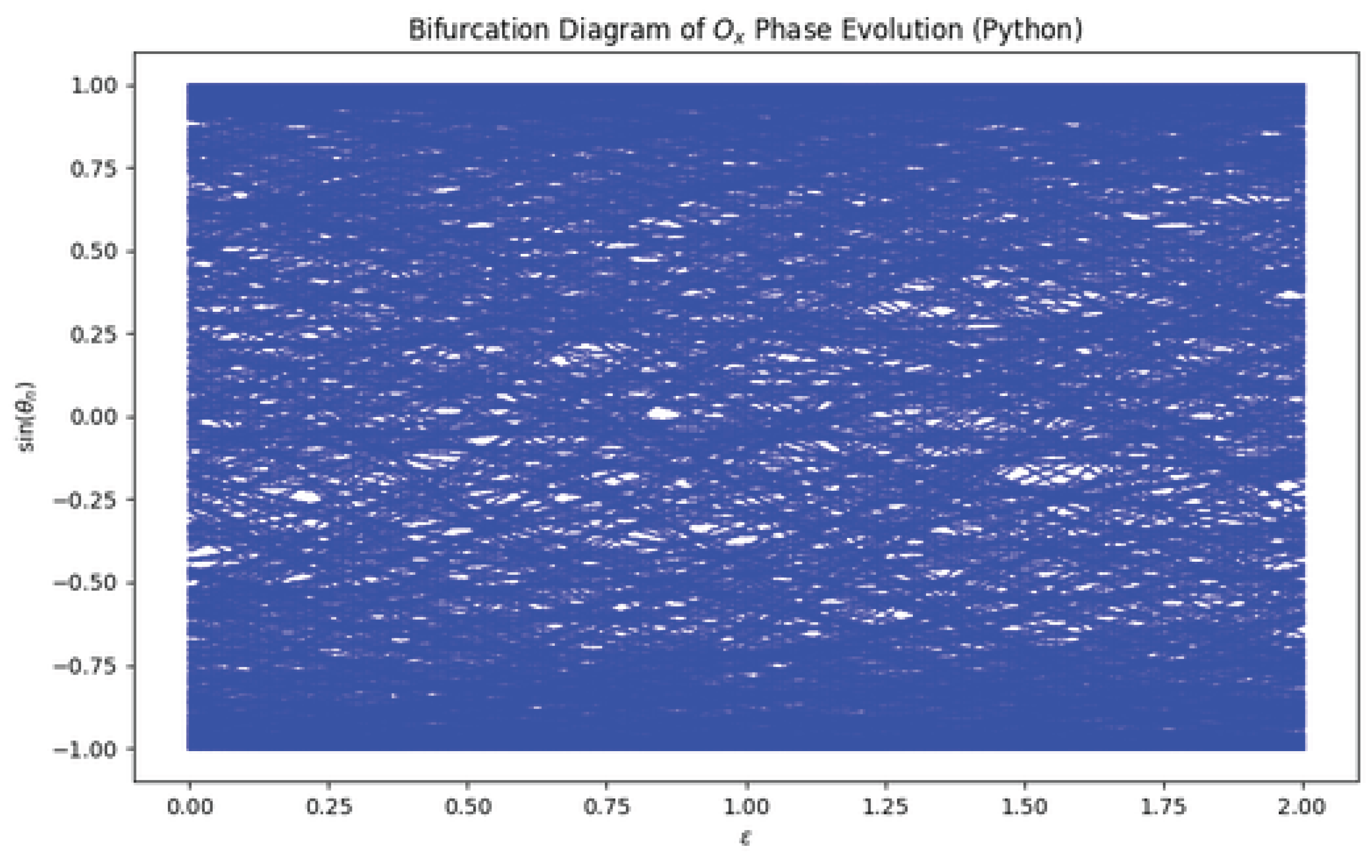
Figure 3.
Lyapunov exponent of the chaotic operator as a function of for phase evolution in the critical strip. Simulation parameters: , , , . Negative exponents indicate stability with closed and homoclinic-like orbits reflecting confined zero dynamics.
Figure 3.
Lyapunov exponent of the chaotic operator as a function of for phase evolution in the critical strip. Simulation parameters: , , , . Negative exponents indicate stability with closed and homoclinic-like orbits reflecting confined zero dynamics.
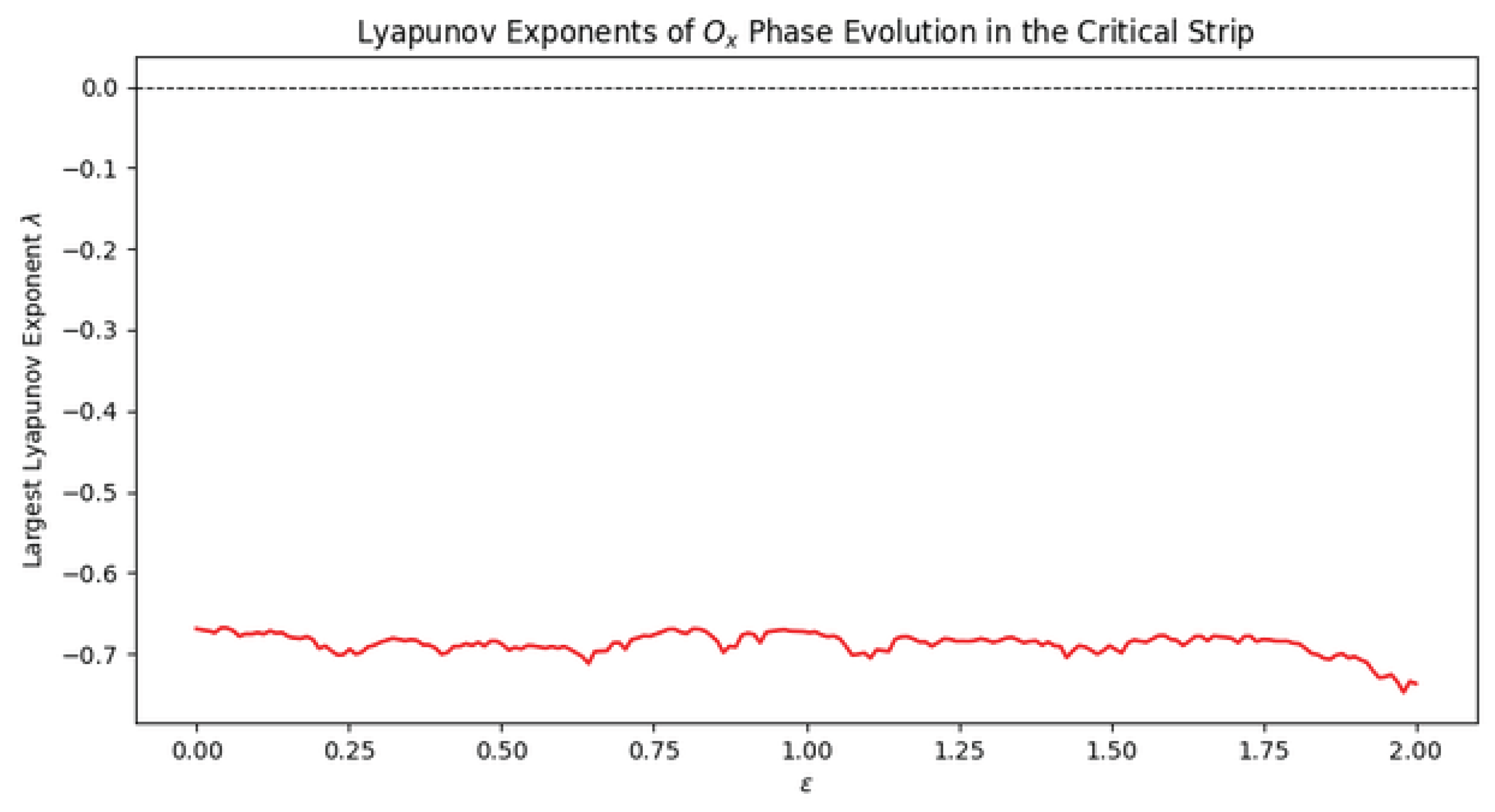
Figure 4.
Mandelbrot-like set for the chaotic operator with perturbation . The iteration was run with 200 iterations, escape radius 2, and grid resolution . The irregular, fuzzy boundary reflects chaotic influence and mirrors the delicate, highly sensitive structure of zeta zeros in the critical strip.
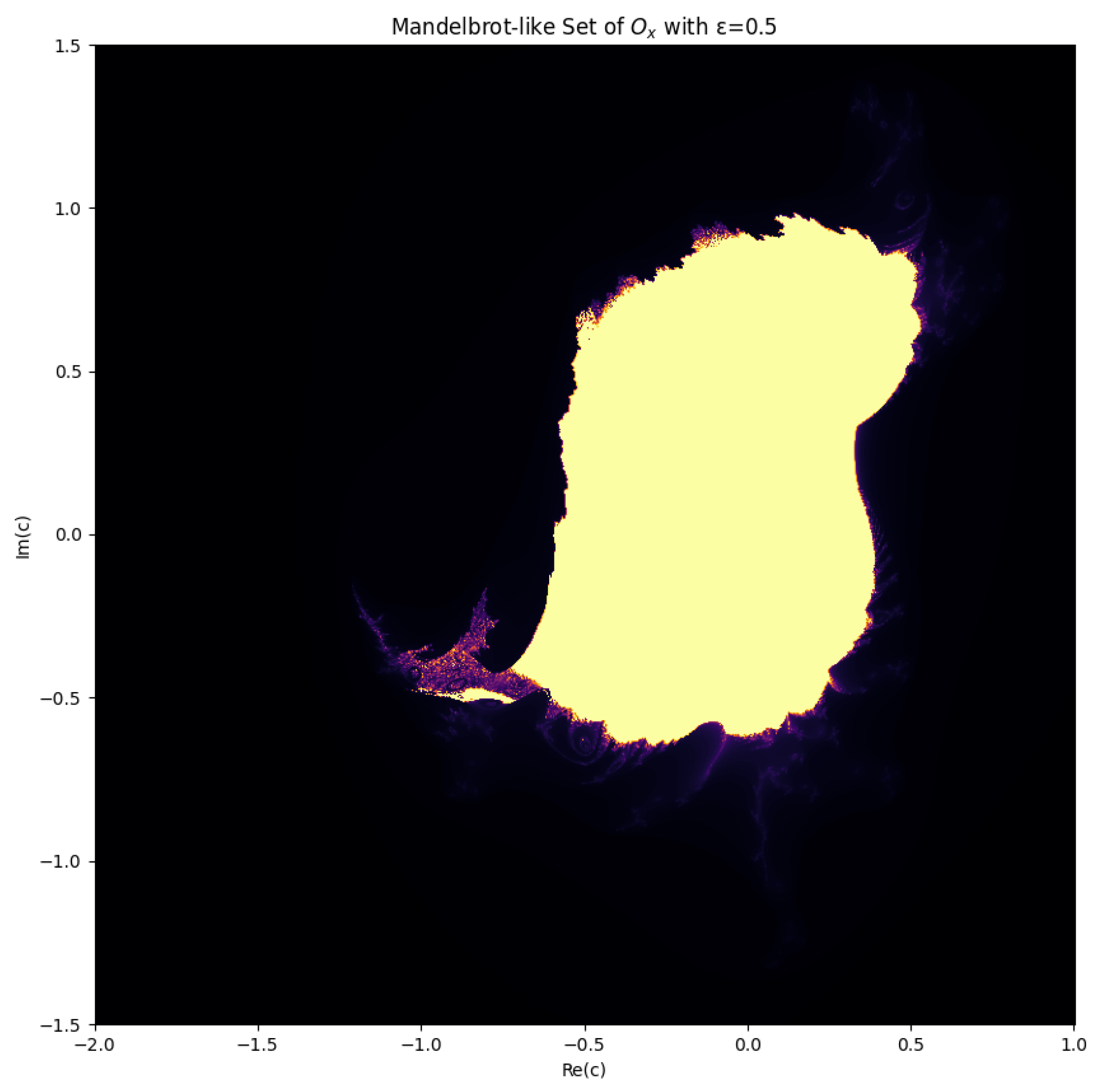
Figure 5.
Julia set of the chaotic operator for and . Points that remain bounded under the perturbed iteration form the dark fractal region, while colors encode the escape time of divergent orbits. The iteration used a grid of points, escape radius 10, and 200 iterations. The intricate, filamented structure reflects the sensitive and complex dynamics analogous to the behavior of Riemann zeta function zeros in the critical strip.
Disclaimer/Publisher’s Note: The statements, opinions and data contained in all publications are solely those of the individual author(s) and contributor(s) and not of MDPI and/or the editor(s). MDPI and/or the editor(s) disclaim responsibility for any injury to people or property resulting from any ideas, methods, instructions or products referred to in the content. |
© 2025 by the authors. Licensee MDPI, Basel, Switzerland. This article is an open access article distributed under the terms and conditions of the Creative Commons Attribution (CC BY) license (http://creativecommons.org/licenses/by/4.0/).
Copyright: This open access article is published under a Creative Commons CC BY 4.0 license, which permit the free download, distribution, and reuse, provided that the author and preprint are cited in any reuse.


