
Submitted:
05 August 2025
Posted:
06 August 2025
You are already at the latest version
Abstract
Decentralized security architectures powered by distributed ledger technology (DLT) have become prominent solutions for elevated security in Web 3.0. The IOTA Tangle is an open-source DLT, available for the Internet of Things (IoTs), as transactions can be carried out freely. IOTA 2.0 is the recent version of the IOTA Tangle, yet its local snapshot mechanism has certain drawbacks — security violations, increased costs and a lack of centralized coordination. Specifically, the situation-unaware decision for pruning increases the cost for energy service providers in the smart meter setting. Data analytics becomes infeasible due to the localized pruning policies. To address these issues, we develop a deep-Q actor-critique network-based cooperative pruning algorithm for IOTA 2.0 that preserves cryptographic properties for stored data in every edge server, namely, first and second preimage resistance, collision resistance and integrity. Our informal security analysis against active adversaries reveals the satisfaction of the security properties. Extensive simulation using the Monte Carlo method unveils that the proposed method is efficient regarding 30% improvement in storage reduction and 35% improvement in energy reduction, committing to the lower bound in solution. Our study quantifies the cost benefits of the proposed algorithms for five random cities with varying population densities for the years 2025 to 2029. We implement and test the algorithms in a real-world setting to benefit diverse stakeholders. Our solutions can be adopted by energy companies for cost-benefit and the IOTA Tangle foundation for future up-gradation of its snapshot mechanism.
Keywords:
IOTA tangle
; Web 3.0
; blockchain security
; blockchain for IoT
; smart meters
; energy trading
1. Introduction
Web 3.0 is the next evolution in Internet technology, shifting the paradigm of centralized trusted architecture to decentralized architecture with the utility of Artificial Intelligence [1]. Blockchain is the underlying technology in Web 3.0 that fosters decentralized trust on the Internet, controlling identities and data by users rather than companies. Smart contracts, decentralized finance, and bitcoin are examples of blockchain applications [2]. Industries are adopting blockchain in their service architecture as it facilitates a unique dimension of user autonomy. Blockchains are categorized into three types: public, private and consortium. The public blockchain is decentralized and open, such as Bitcoin, Ethereum and Solana. The private blockchain is permissioned. For example, Hyperledger Fabric, Alibaba blockchain, IBM blockchain, Microsoft Azure blockchain, Meta blockchain and Google Cloud blockchain are private blockchain offerings from big tech companies. The consortium blockchains, like R3 Corda and Quorum, are partially decentralized. Needless to say the sole purpose of blockchain is lost when they are offered as a service on a payment basis. However, targeting the Internet of Things (IoTs), the IOTA Tangle is an open-source Distributed Ledger Technology (DLT) where there are no miners and chargeable transactions like Ethereum 1. Especially, as the transactions (smart meter readings) and utility are not charged, anyone can use the stack to avail of free blockchain in their service architecture. On the flip side, it is under development, which means that people are actively researching to improve it from known vulnerabilities and bottlenecks in deployment [3].
Differing from the traditional blockchain with the proof of work (PoW) and Proof of Stake (PoS), the IOTA Tangle works by Directed Acyclic Graph (DAG). Every transaction in the Tangle network is referred to as a site (approved). Accordingly, the first approved transaction is the genesis site in the network. To add new transactions in the Tangle, transactions are locally verified (signature) by a node. To add the verified transactions (site) in the network, the local node attaches the transaction (tip) to two sites with the tip (not yet approved). Thereafter, the Tip Selection Algorithm (TSA) executes the process to approve the tip in order to convert it to a site [4]. It is noted that every site in the Tangle carries the specifics of a traditional blockchain, say transaction hashes, block signature and Merkle root. The recent version of the IOTA Tangle is IOTA 2.0 (Coordicide), and its previous version is IOTA 1.5 (Chrysalis). Using conventional blockchain for the energy industry is in practice [5], and its applicability is even wider, starting from the energy-producing sector to the energy-selling market [6].
We consider a network architecture with the IoT setting, shown in Figure 1 where the smart meters from homes and industries are connected to the edge servers via LORA technology. The edge servers are rented by the energy companies from cloud service providers (CSPs), such as Amazon Web Services (AWS), Microsoft Azure, Oracle Cloud and Google Cloud. CSPs and energy companies are in a software-level agreement (SLA). Energy companies utilize IOTA 2.0 as the blockchain architecture (Tangle network) to offer services, like smart contracts and smart meter users. Particularly, the Tangle network utilizes a deep Q actor-critic network-enables a reinforcement learning algorithm, where the actor (DQ-AN) and critic (DQ-CN) jointly work to obtain the optimal policy of storage, energy and pruning frequency. By pruning, we mean removing expired blocks. For this, an agent trains the network to minimize the loss by updating the parameters, and the agent works in a model-free architecture using the replay memory as a minibatch for sampling the (state, action, reward) tuple. Our architecture is an extension of the blockchain architecture considered for the smart meter application [7]. Notably, blockchain technology is widely applied in the energy sector, focusing the energy trading [8].
When IOTA 2.0 is utilized, energy providers cannot attain security, cost-effectiveness, and data analytics capability, which are prominent in securing the network and offering sophisticated services to users from the supplier’s point of view. For optimizing the network, the pre-Chrysalis version used the global snapshot mechanism, facilitating network-wide coordination. The global snapshot requires a coordinator to carry out the task, and it demands network-wide consistency to attain the pruning. Nonetheless, IOTA 2.0, is upgraded by the local snapshots where individual nodes can execute the pruning to optimize the storage 2. Though the local snapshot mechanism solves the issue of the requirement for a global coordinator and the process for maintaining network-wide unanimity, further improvement is still required to safeguard the security of the network. Specifically, the local snapshot is governed by static rules, i.e., nodes execute the pruning decision when the threshold limit for the storage is reached locally. This decision can lead to over-pruning or under-pruning, violating the storage requirement of minimum transactions to safeguard the security of the network. Also, as the global snapshot is deprecated in IOTA 2.0, we highlight that the lack of a coordinator can lead to failure in data analytics, blocking the utility of machine learning methods for electricity price forecasting [9]. Figure 2 shows the problems associated with the local snapshots and how they are overcome in the proposed method by the Actor-Critic-based Deep Q network. Considering the challenges faced by the local snapshot mechanism in IOTA 2.0, we pose the following question: "How can pruning decisions in IOTA 2.0 be made secure and efficient in decentralized edge networks?" This research question opens avenues to solve the problem in two-fold: developing methods to minimize the cost of the energy providers and developing methods to solve the issues associated with the local snapshot mechanism of IOTA 2.0. As optimising the storage directly reduces the number of edge servers and imposing security constraints while reducing the storage prevents the adversarial attacks, this research question is worth solving.
By answering the research question, we lay out the following contributions of this article:
- We formulate the cost optimization problem as a function of the storage, energy and pruning frequency optimization for optimizing the policy of energy and storage consumption and pruning frequency, respectively. Precisely, we optimize storage and energy by strictly satisfying security constraints in sub-problem 1. Then, we jointly optimize the pruning frequency in sub-problem 2, where constraints are relaxed to attain a feasible solution.
- We develop Actor-Critic method-based deep reinforcement learning algorithms (DQACN) for deep policy optimization, working cooperatively when they are deployed in the edge servers with a cloud service provider.
- Extensively, we perform the Monte Carlo simulation to gain confidence in the performance improvement of proposed algorithms over conventional local snapshots, global snapshots, ordinary deep Q network and random elimination methods.
- We implement and test the proposed algorithms to evaluate their performance robustly in the real-world environment.
The remainder of the article is organized as follows: Section 2 presents the related work. Section 3 presents problem formulation, introducing IOTA 2.0. Section 4 put forth the solution approach, convergence proofs for the proposed algorithms and formal security analysis in the universal composability framework. The next section (Section 5) evaluates the proposed algorithms and other methods using the Monte Carlo simulation. Section 6 carries out the implementation study of the proposed algorithm in a real-world setting. Finally, the work is concluded in Section 7.
2. Related Work
Aiming to present the taxonomy in storage optimization of the blockchain, the study [10] categorizes storage optimization in blockchain into three types: replication-based, redaction-based and content-based. Storage optimization in conventional blockchains is targeted by replication-based methods, whereas the redaction-based and content-based methods find optimization in the service and application layers. This study clarifies that storage optimization in the IOTA Tangle has not been done, so we take our breadth-first approach towards optimizing the storage and its associated cost in the IOTA Tangle by preserving security.
Xu et al. [11] presented the storage optimization in blockchain. Their work formulates the objective function as a multi-objective function, and their storage model captures the disk space of the servers used in the cloud environment. However, they propose the genetic algorithm-based solution approach, which usually takes a longer time to find the global optimum solution.
Zuo et al. [12] put forth a three-level, involving IoT devices, a base station and a cloud server, Stackelberg game-based optimal cloud resource utilization model involving IoT devices, base station, and cloud server. This method shows how to cooperatively allocate cloud resources for blockchain storage. Moreover, it lays out the resource allocation model, computing service pricing model and computing, storage and communication model. This work captures mining in the blockchain; however, their work does not involve optimizing the blockchain itself, which directly contributes to the storage space.
Targeting the minimization of energy consumption and carbon emission, Alofi et al. [13] studied the multi-objective optimization for the Bitcoin environment. Their work considers a variety of objectives ranging from reputation to carbon emissions. They present the Pareto front for the different combinations of objective functions, minimizing the convex function with the obtained hypervolume set. Nonetheless, they used the evolutionary algorithm as the solution approach, which takes a longer time to converge and is unsuitable for the considered application in the edge-based cloud network.
Akrasi-Mensah et al. [14] discussed the usage of the deep reinforcement learning algorithm for solving storage optimization in the cloud. Specifically, they considered a blockchain network for the cloud where storage cost is optimized. The solution approach consists of an Actor-Critic method-based optimal policy selection algorithm. Though this approach presents the applicability of the deep reinforcement algorithm as the solution approach, this method does not consider edge networks, i.e., the method applies to the traditional cloud network model.
Zhou et al. [15] presented a way of optimizing the storage cost in the blockchain. The problem is formulated as a multi-objective optimization and reduced to the block selection problem. For optimizing the blockchain, the storage model captures the blockchain as individual blocks with a finite size. Their solution approach considers the traditional deep Q network, which overcomes the curse of dimensionality in the conventional reinforcement learning methods. However, the blocks in the blockchain do not capture the nuance of transactions, signatures and the Merkle root of the block, which is essential to assess the security of the optimization.
Considering a consortium blockchain network, Tanis et al. [16] proposed a cooperative framework for energy trading using the Nash equilibrium [17]. In contrast to the traditional single-energy model, this work takes into account the multi-energy model. Q-algorithm in reinforcement learning is used to solve the nonlinear multi-objective optimization. However, this work does not consider storage optimization, though it leverages the cooperative framework.
In general, in the storage optimization of the blockchain and the granularity of modeling the blocks (precise modeling of components of a block/site) in the blockchain are absent, though optimization for improving throughput is evident [18]. Importantly, security constraints have not been considered to preserve security. Further, blockchain optimization for the edge-assisted cloud network has not been considered, specifically implementing the IOTA Tangle. Cost optimization for energy service providers renting the cloud server from CSPs using the IOTA Tangle network is not reported in the literature, which is a thriving market.
3. Problem Formulation
In this section, we formulate the energy model and storage model of IOTA 2.0 (Coordicide), followed by formulating optimization problems for energy cost, storage cost and pruning frequency. While IOTA 2.0 does not use the proof of work of the traditional blockchain, it retains many features of the blockchain, such as signature computation and Merkle root retention for transactions (sites), so we introduce the features of IOTA 2.0 and compare them with the conventional blockchain. Then, we prove that the presented optimization problem is NP-hard.
3.1. IOTA 2.0 (Coordicide)
IOTA 2.0 is referred to as a Tangle rather a blockchain since the network is formed by a DAG. Transactions in IOTA 2.0 are called sites. Each site is referenced by two previous transactions (tips). When a node wants to add a transaction, it places the site (unapproved transaction) in the tangle by referring to two previous tips (approved transactions). Then, the Tip Selection Algorithm (TSA) approves the added site to a tip with the help of the referenced two tips. Thus, every site in the tangle is referenced by two tips.
The proof of work is replaced by the mana-based system and Fast Probabilistic Consensus (FPC). Mana is a reputation-based resource bound with every node. This is introduced to have a full-fledged decentralization, as the coordinator in the previous version (IOTA 1.5) is replaced. Every node generates mana by holding IOTA tokens (stake-based) and through its activity (transactions). There are two types of manas, viz, access mana and consensus mana. The access mana determines the node’s access to the network, that is, the number of transactions issued by the node. Consensus mana defines the weight of the node when it participates in voting during FPC. The mana of a node is used for at least three purposes: protection, control and weighing. Briefly, Mana prevents the Sybil attack by giving importance to token ownership. This prevents malicious nodes from gaining disproportionate access in the tangle by creating fake identities. Mana regulates the transaction issuance rate. Nodes with higher mana are preferred during network congestion. Consensus mana of every node carries wight during voting in FPC. That is, nodes with higher consensus mana have an advantage in conflict resolution as their votes are weighed higher. Table A1 (Appendix B) compares IOTA 2.0 with the proof of work (PoW) and proof of stake (PoS) of the traditional blockchain.
Remark: While the coordinator (centralized and recommended in IOTA 1.5) is deprecated in IOTA 2.0, deployment of the global coordinator has some benefits. For instance, aggregated data retention for future data analytics can be easily accomplished with such a central coordinator though it does not hold any important roles centrally, like the global snapshot (pruning decision is centrally coordinated).
3.2. Energy Model
Let the total number of edge servers be . Out of the edge servers, a subset of servers () is responsible for carrying out FPC. Table 1 elaborately presents the different notations and their meaning. The pruning decision for optimizing the storage relates to energy consumption.
The cost for edge servers rented by the energy companies depends on the energy consumed by the tangle network. Therefore, it is essential to precisely model the energy cost associated with the tangle network. Without loss of generality, we present the energy cost for the tangle network as the cost incurred for transaction, tip, consensus and pruning.
The total energy consumption across all edge servers at time n in IOTA 2.0 is given by.
The cost associated with a transaction can be decomposed into the cost incurred for the hash computation, signature computation, attaching cost and the number of transactions. Accordingly, Equation (2) presents the transaction cost for the server.
The consensus cost is presented in Equation (3).
where denotes the mana, and it is given in (4). We assume the smart meters delegate their mana to the edge servers (pledging) as they have limited computing resources. The mana of server i at time n is updated to include pledged mana from the smart meters in the below equation that presents the time evolution model of the mana. This equation, also, captures the notion of decreasing mana of a server in the event of inactivity.
The energy associated with tip selection for server i at time n in IOTA 2.0 can be expressed as follows:
The energy associated with pruning operations (local snapshot pruning in IOTA 2.0) for server i at time n in IOTA 2.0 is given by:
3.3. Storage Model
The storage dynamics over time are captured by the storage model of the time evolution equation. For the discrete time instance n, the storage is given by , i.e., storage contributed from the previous time instance, where . Equation (9) depicts the total storage contributed at n by the server, where and denotes the storage size per transaction and coefficient for the transaction of the server, respectively.
The quantity of storage freed by pruning is modeled in the Equation (10). specifies the storage cost eliminated by pruning, and denotes the act of pruning done at the server at the instance n.
3.4. Problem Formulation
In this study, our aim is to optimize storage and energy as they directly contribute to the cost of an edge server, thereby increasing the monetary benefit. The key performance indicator of the objective function is linked to the cost-benefit. While optimizing the storage and energy, constraints, namely security constraints, software level agreement (SLA), bill settlement and retention of historical data have to be strictly satisfied. Therefore, we formulate sub-problem 1 (SP 1) to optimize the storage and energy by strictly meeting these constraints (constraint satisfaction problem (CP)). Sub-problem 1 is formulated to optimize storage and energy individually. Then, in the sub-problem 2 (SP 2), we jointly optimize the pruning frequency, energy and storage. We formulate each objective function using regret, as the regret-based formulation captures dynamic scenarios in comparison with the usual static formulation. The proposed optimisation is replication-based.
In the above equation, represents the cost at time t, and specifies the best possible cost in hindsight. By Equation (14), we intend to minimize the energy consumption by choosing the best policy from the set of policies , where , i.e. a mapping function from state to action (refer to next section).
SP 1:
Security constraints for a 256-bit security level are presented in . In , presents the security constraint for the first preimage resistance (given a hash, finding its input is computationally infeasible). This constraint imposes search space complexity bounded to computation time for a hash (), i.e., when time , . presents the security constraint for the second pre-image resistance, that is, given a hash and its input, finding its second input is computationally infeasible. presents the constraint for collision resistance property, that is, finding two distinct inputs for the same hash output is computationally infeasible. Due to the birthday paradox, is reduced to . presents the integrity constraint. We assume that 1 billion hashes can be produced in a second, though in Bitcoin mining, 1 trillion hashes per second are produced. Accordingly, the minimum values obtained are in the order of . For the integrity, the maximum value is obtained in the order of as IOTA 2.0 uses Winternitz One-Time Signatures (WOTS), which accounts for 1 million signature verifications per second. presents the pruning constraints on blocks that are settled for bills. is 1 if the bill is settled; otherwise, its value is 0, indicating not ready for pruning. presents the number of blocks retailed as part of the historical data. Constraints from to present software level agreement (SLA) constraints. Electricity and cloud service providers agree on an SLA to rent resources. Specifically, depicts the storage capacity of the edge server should not exceed its maximum capacity. presents the constraint that at the cloud level, the minimum storage has to be ensured for future audits. insists the pruning frequency should not exceed its limit as it increases energy consumption. presents at the cloud, minimum storage has to be ensured for analytics purposes. ensures the retention of local historical data for the smart meter.
Now that we present the objective function based on the regret definition (refer to Equation (13)) for energy optimization.
ensures the minimum energy is allotted to maintain security. In particular, ensures energy consumption for the first pre-image resistance. assures the energy consumption for the second pre-image resistance. ensures the energy consumption for maintaining the collision resistance property. warrant the energy consumption for maintaining the integrity. confirms only if pruning is allowed bill after bill settlement. corroborates that energy is allotted for retaining the relevant blocks as historical data. and meet the energy consumption of the edge server does not exceed its maximum capacity, and the energy capacity of the cloud is allotted to meet its minimum energy utilization. The pruning frequency should not consume much energy. This is met in . While allocates the minimum energy consumption for maintaining the historical data, prevents that energy reduction from falling below the minimum level of energy for maintaining the historical data. The final constraint ensures the balance between the energy used by cloud and edge w.r.t. the energy maintained for retaining historical data.
SP 2:
We jointly optimize the pruning frequency by considering the energy consumption and storage consumption costs, and turning security constraints into the objective function.
In Equation (16), , and are weights for energy consumption, storage and security at time n, respectively. and are energy and storage at hindsight. is the objective function capturing the security constraint. is the objective capturing the security constraints. Precisely, the first pre-image resistance term is covered in . The second pre-image resistance is absorbed by the term . The collision resistance and integrity are modelled by the terms and , respectively. are the weights for these security properties. From Equation (18), is the best known pruning frequency at hindsight. Equation (18a) imposes a constraint for pruning energy, i.e. total pruning energy should not exceed the maximum energy. The pruning should not be overwhelmed, and it is met in the constraint (18b) by ensuring minimum blocks. At any instance, should be more than the number of blocks retained as historical data (Equation (18c)).
We show that SP 2 is NP-hard as it includes SP 1 and its components as constraints. The problem of finding the optimal pruning frequency is an NP-hard problem. We prove that the Pruning Optimization Decision Problem (PODP) is NP-hard by reducing it to the Boolean Satisfiability Problem (SAT), which is NP-complete (PODP is polynomial-time reducible to SAT).
Decision Problem formulation: Given N edge servers, time slot T, pruning decisions , costs , and threshold K, does there exist a pruning schedule such that:
subject to the constraints of SP 2. The proof is presented in Appendix A.
4. Solution Approach Based on Deep Q Actor Critic Network (DQACN)
Figure 3 depicts the architecture of the deep Q actor-critic network in which the actor network is optimized by the gradient ascent method, and the critic network is optimized by the gradient descent method. Initially, the agent observes the state of the environment, and it utilizes the actor network. (policy function network) to take action based on transition probabilities. The action is applied to the environment, resulting in a new state and reward. Then, the critic network evaluates the new state value and current state value by computing the temporal difference (TD) error, followed by tuning the critic and actor networks. The problem of selecting a random server is solved by using the SoftMax probability function , i.e., this function turns the energy cost of every server into the probability distribution, where servers can be selected by knowing their lowest probability score. Once the server is selected, it is allowed to solve optimization problems in order to find the cost-efficient storage, energy and pruning frequency. The server broadcast its solutions to the remaining servers. The recipient servers check whether the received solutions satisfy the constraints. If the constraints are satisfied, then other servers accept the current solution; otherwise, they reject the new solution. Once the pruning is executed locally, the edge server updates the retained data to the rented cloud server, facilitating future data analytics.
Now, we present the state encoding variables, action space encoding variables, and reward and penalty to deploy the deep Q actor-critic network-based agent, representing the environment. The state for server k at time n is defined as follows, and it is common for SP 1 and SP 2. Note that for the mana state, we consider the old value and the recent value, as backlog and finalized, respectively:
The action space server k at time n is defined for SP1 and SP 2 as:
The reward for the agent is defined as the negative of the total cost minus a penalty for violating constraints. For SP 1 and SP 2, the reward is defined as below.
Let the total cost be .
- For Algorithm 1 (SP 1):
- For Algorithm 2 (SP 2):
The penalty term accounts for violations of key constraints, e.g., security constraints. This ensures that the agent chooses the appropriate pruning frequency by respecting constraints and other objectives.
We brief out the working of Algorithm 1 and Algorithm 2. We note that Algorithm 1 must be executed to preserve the security, before Algorithm 2 is executed. Algorithm 1 solves SP 1, thereby producing the solution for optimal storage and energy cost. Then, Algorithm 2 consumes the solution of Algorithm 1 and produces the optimal pruning frequency. We discuss the generic layout of Algorithms 1 and 2. At first, parameters are initialised, and the softmax probabilities are calculated for the edge servers. Then, storage and energy in hindsight are proposed, and the regret for those is computed. If the regrets for the storage and energy are non-negative, it is discarded. Otherwise, the solution is accepted. Then, the actor and critic networks are updated, and this process is iterated for the maximum number of iterations. In Algorithm 1, the parameters of the actor-critic network are initialised in all edge servers (Steps 3 to 6). Among the edge servers, a server () is selected (Steps 8 to 11) by the choice of SoftMax probability function (Step 10). Steps 13 and 14 present the environment to the agent (now, server). Using the storage and energy equations, the agent proposes a new value for the storage and the energy by respecting the strict constraints (Steps 15 and 16). In Steps 17 and 18, the agent evaluates the regret. The agent finalises the storage and energy value in Step 19, which is broadcast to other servers. From Steps 21 to 28, other servers evaluate the solution, i.e. whether the new value for the storage and energy satisfies the constraints. The solution is accepted by the remaining servers if the constraints are satisfied (from Steps 29 to 33). In Step 35, the agent computes the advantage function as the computation of the temporal difference learning (the function is computed by targeting future reward as the dominant factor rather than the immediate reward). Additionally, the agent works out such a step by bootstrapping. Step 36 shows the gradient descent step of the critic network with the learning rate (), whereas Step 37 shows the gradient ascent step of the actor network. At last, the agent outputs the storage and energy values. Note that here the value of the pruning frequency is still null, and it is solved in Algorithm 2. Until Step 11, the agent follows the steps of Algorithm 1. In Step 14, the agent turns the security constraints into part of the objective function. Step 18, additionally, includes the pruning frequency. In contrast to Algorithm 1, the agent updates its actor and critic network parameters after Step 29 by evaluating the advantage function. Then, the new solution is broadcast to the remaining edge servers. From Steps 30 to 38, the edge servers are updating their actor and critic parameters as per the received solution. Finally, every edge server gets the updated storage value, energy value and pruning value.
Next, we analyse the convergence of the algorithms to depict whether the algorithms attain such solutions in sub-linear time, as the regret assures such efficiency.
| Algorithm 1 Storage and Energy Optimization (SP 1) with Softmax-based Random Server Selection and Actor-Critic Evaluation |
|
| Algorithm 2 Joint Pruning Optimization (SP 2) with Softmax-based Random Server Selection and Actor-Critic Evaluation |
|
4.1. Convergence Proof
While the deep Q actor-critic-based method is used for solving optimization problems in different contexts, we attempt to present the formulated regret functions indeed converge to the optimal solution in sub-linear time.
We present the assumption for proving theorems in Appendix A.
Theorem 1.
Under the assumptions of finite state and action spaces, bounded rewards, Robbins-Monro learning rates, and an ergodic MDP, Algorithm 1 converges to a locally optimal policy for SP1, minimizing energy and storage costs subject to constraints to , with sublinear regret .
The proof of this theorem is presented in the appendix section (Appendix A).
Theorem 2.
Under the assumptions of finite spaces, bounded rewards, Robbins-Monro learning rates, an ergodic MDP, Lipschitz continuity, and bounded security costs, Algorithm 2 converges to a locally optimal policy forming a Nash equilibrium for SP2, jointly optimizing pruning frequency, energy, and storage, with sublinear regret .
The proof is presented in Appendix A.
Now, we show that the proposed algorithm for SP 1 truly satisfies security properties, namely, first pre-image resistance, second pre-image resistance, collision resistance and integrity against active adversaries.
4.2. Adversary Model
We consider the Dolev-Yao adversary model for the adversary . can overhear communications between the smart meters and edge servers, taking the passive role. The attack surface for the adversary is considered at the edge servers. In the active role, can substitute fake transactions in the storage held at every edge server. The adversary can violate the first preimage resistance, i.e., it can find the inputs for a targeted hash. By violating the second preimage resistance property, can identify the other inputs that share the same hash value. In the event of breaking the collision resistance property, the adversary can find other inputs for a targeted input and hash. While counterfeating the integrity, can substitute fake transactions to claim that they are legitimate.
4.3. Formal Security Analysis
We formally analyze how Algorithm 1 safeguards security against a classical active adversary using the universal composability framework, so we start with the relevant terminology of the framework. We claim the sense of security for the only properties claimed in the below propositions. The security is attained by satisfying the properties.
- Real World: Parties execute the protocol (Algorithm 1) in the presence of an adversary .
- Ideal World: Parties interact with an ideal functionality that securely implements the desired behavior, with a simulator emulating the adversary.
- Security Definition: A protocol UC-realizes if, for any adversary , there exists a simulator such that every environment cannot distinguish the real-world execution (with and ) from the ideal-world execution (with and ).
Refer to Appendix A for the ideal functionality ().
- Proposition 1: Algorithm 1 ensures the first preimage resistance with non-negligible probability.
- Proposition 2: Algorithm 1 satisfies the second preimage resistance with non-negligible probability.
- Proposition 3: Collision resistance with non-negligible probability is achieved by Algorithm 1.
- Proposition 4: Integrity with non-negligible probability is ratified by Algorithm 1.
We prove the propositions by showing that Algorithm 1 UC-realizes , satisfying the respective security property (refer to Appendix A for the proofs).
5. Simulation and Analysis
In this section, to asses the effectiveness of the proposed algorithms, we ask the following sub-research questions (SRQs):
- SRQ 1: How much efficiency is attained by DQACN (Algorithm 1 and Algorithm 2) w.r.t. the local snapshot mechanism in IOTA 2.0?
- SRQ 2: How far do DQACN (Algorithm 1 and Algorithm 2) satisfy the constraints strictly?
- SRQ 3: What is the cost-benefit of the proposed algorithms over local snapshot in IOTA 2.0?
To answer SRQ 1, we perform the Monte Carlo simulation as per the network setting of IOTA 2.0. Moreover, we simulate the network behavior of the IOTA 2.0 to capture the actual effectiveness of the proposed algorithms. We consider the local and global snapshots supported in IOTA 2.0 and IOTA 1.5, respectively, and the deep Q network and random elimination methods for comparison.
We consider a random process of transactions sent by the smart meters received by edge servers, with the IOTA Tangle network between smart meters and edge servers. We capture the input variables with the appropriate probability distribution, modeling the activity of the mana with the appropriate probability distribution.
Refer Appendix C for the probability distributions considered for the random process.
We use the values specified in Table A3 for different parameters. As we considered the temporal difference learning method in the actor-critic network, the network learns the optimal policy by bootstrapping (initial guess followed by iterative refinement), attaining convergence in the critic network. Figure 4 presents the simulation result. 1 in Figure 4 demonstrates the total cost, whereas Sub-figures 2 and 3 show the storage and energy costs, respectively. In the three sub-figures, Algorithm 2 (Alg 2) outperforms all schemes, typically consuming lower cost than the local snapshot. Sub-figure 1 depicts the total cost w.r.t. increasing edge servers, summing the energy cost and storage cost presented in sub-figures 2 and 3, respectively. When the edge server reaches 100, Algorithm (Alg 1) attains approximately 50% cost reduction in comparison with the local snapshot as it is driven by the static pruning rules. Alg 2 shows the cost reduction of 60% when compared with the local snapshot. This reduction trend is reflected in the ordinary deep-Q network as well; however, the actor-critic-based method outperforms all methods, namely local and global snapshots, random elimination and deep Q method.
In Sub-figure 2, the proposed algorithms’ storage cost is almost zero for proposed algorithms because of the aggressive pruning frequency. This trend shifts for increasing servers due to the time evolution model of the storage function and security constraint satisfaction. Sub-figure 3 demonstrates the energy cost of the proposed algorithms, showing lower consumption of energy. Notably, Algorithm 2 consumes the least energy, whereas the global snapshot incurs the highest energy cost. Remaining methods contribute to the middle values between the proposed algorithms and the global snapshot.
Sub-figure 4 shows the amount of pruning frequency versus the number of servers where the highest values are attained by the random elimination since the pruning decisions are not cost aware; however, the least value comes from the local snapshot because of static rules, say prune only if the storage capacity exceeds 85% of the total storage. Proposed algorithms have higher pruning frequencies to optimize the storage and energy costs.
Sub-figure 5 shows the total cost in relation to transaction volume, with Algorithm 1 performing best by minimizing costs, followed by Algorithm 2 in energy consumption. Sub-figure 6 indicates that both Algorithms 1 and 2 achieve the same lowest storage cost. Sub-figure 7 highlights that Algorithms 1 and 2 outperform others in energy costs. Regarding pruning frequency, the local snapshot shows the lowest costs, but effective pruning decisions are necessary for optimal savings, leading to a higher pruning frequency in the proposed algorithms. Sub-figures 9, 10, and 11 demonstrate the quick convergence of pruning decisions for total cost, storage cost, and energy cost in the proposed algorithms compared to others.
SRQ 2 is answered in Sub-figure 12. For all the pruning decisions, Algorithm 1 strictly satisfies all constraints. Algorithm 2 occasionally satisfies the constraints, whereas the remaining methods, such as local and global snapshots, and the deep Q method, do not satisfy constraints, resulting in security violations and infeasibility in data analytics.
We answer SRQ 3 as follows. We consider five cities, namely Amsterdam, Beijing, Cincinnati, Delhi and Milan for our study. The profile of the cities, including population, smart meter usage, number of edge servers used and renting rate, are depicted in Table A4 (Appendix C). We present the case for Amsterdam. For all cities, we consider the rental rate of the edge server as 5000 USD/year (Appendix C).

Table 2.
Average Cost Savings Using Algorithms 1 and 2 for Smart Meters in Five Cities (USD, 2025-2029).
Table 2.
Average Cost Savings Using Algorithms 1 and 2 for Smart Meters in Five Cities (USD, 2025-2029).
| City | 1-Year | 2-Year | 3-Year | 4-Year | 5-Year |
|---|---|---|---|---|---|
| Amsterdam | 5,585,700 | 11,171,400 | 16,757,100 | 22,342,800 | 27,928,500 |
| Beijing | 136,652,240 | 273,304,480 | 409,956,720 | 546,608,960 | 683,261,200 |
| Cincinnati | 1,857,440 | 3,714,880 | 5,572,320 | 7,429,760 | 9,287,200 |
| Delhi | 204,978,360 | 409,956,720 | 614,935,080 | 819,913,440 | 1,024,891,800 |
| Milan | 8,693,120 | 17,386,240 | 26,079,360 | 34,772,480 | 43,465,600 |
6. Implementation Study
In this section, we implement the proposed algorithms to answer the following research question.
SRQ 4: What is the effectiveness of the proposed algorithms in the actual edge server environment?
SRQ 5: How do energy and other industries, and the IOTA community benefit from this research?
To answer SRQ 4, we consider the following environment for implementing and testing the proposed algorithms: Linux (operating system type), x86_64 (processor), Intel(R) Xeon(R) CPU @ 2.20GHz (processor brand and operating frequency), 12 GB (RAM) and 2 (CPU cores). We use Python 3 as the programming language for the implementation. In order to assess the proposed algorithms in a real-world setting, we implement the IOTA node with mana and the DQACN agent. We consider the test cases mentioned in Table A2. We test the algorithms to know what extent the storage, energy and pruning frequency are used to understand their baseline operation. For this case, we measure the memory consumed, energy consumed and pruning fraction held initially. To check the robustness of the algorithm towards growing transactions, we subject the second case, which is detailed in Table A2 (Appendix B). To check the security assurance of the proposed algorithms, we use the third test case. To understand the reliability of the algorithms, we use the final test case. Figure A1 (Appendix B) shows the result of the test cases. It is apparent that all of the test cases succeeded, making the proposed algorithms suitable for real-world deployment.
Our developed algorithms can be found in the link 3, and the algorithms can be used for the real-time deployment, or it can serve as the guideline for extended implementation. This answers our SRQ 5. We made the developed algorithms as a standalone file ("dr_agent.py") so that it can be easily used for deployment. Our implementation can be used by the energy companies for the upgradation. Also, the IOTA Tangle foundation can use the developed algorithms as an alternative for the local snapshot.
7. Conclusions
This article identifies key limitations associated with the local snapshot of IOTA 2.0, particularly security violations and the infeasibility of data analytics. We proposed two algorithms based on the deep Q actor-critic network in reinforcement learning. Algorithm 1 optimizes storage cost and energy cost by strictly satisfying constraints (inclusive of security constraints) for a random edge sever, and the solutions are accepted by the remaining servers provided that constraints are satisfied, and Algorithm 2 optimizes pruning frequency without the restriction on the constraint satisfaction. Monte Carlo simulation confirms the practical efficacy of the proposed algorithms. Typically, a significant amount of improvement in efficiency is attained by the algorithms, satisfying security requirements. The study evaluated the cost-benefit of the proposed algorithms by considering five cities. This article studied the real-world implementation of the proposed algorithms and made the algorithms available, ready for real-world deployment. The solutions proposed in this article can benefit the IOTA Tangle foundation for upgrading its future snapshot mechanism. Further, this research can benefit energy companies renting CSPs by following the proposed algorithms over the conventional local snapshot in IOTA 2.0.
Acknowledgments
Funded in part by the European Union (EU), Grant Agreement no. 101095717 (SECURED). Views and opinions expressed are those of the authors and do not necessarily reflect those of the EU or the Health and Digital Executive Agency. Neither the EU nor the granting authority are responsible for them.
| 1 | |
| 2 | |
| 3 |
Appendix A.
Appendix A.1. Proof for the NP-Hardness of SP 2
Proof.
We reduce the problem, beginning from SAT. Given a SAT instance with v variables and m clauses: Set , in Equation (19). Map variable to server . Let if , 0 if . For each clause , the cost is defined as if is not satisfied (all literals false), 0 otherwise. Set . Set . This satisfies constraints.
If SAT is satisfiable, there exists such that all clauses are satisfied (), so , and PODP returns "True". If SAT is not satisfiable, at least one clause is unsatisfied (), so , and PODP returns "False."
The time complexity associated with the construction takes . Since SAT is NP-complete and reduces to PODP in polynomial time, PODP is NP-hard, which is NP-complete. Thus, the optimization problem (SP 2) is NP-hard. □
Appendix A.2. Assumptions
Finite Spaces (A1): To ensure bounded space for the agent, let the state spaces S and action spaces A are finite and discrete [19]. This makes the finite landscape for the agent to explore and make decisions.
Bounded Rewards (A2): Reward r satisfies [20]. This ensures the reward is finite and convergent rather than being divergent.
Learning Rates (A3): The learning rate satisfies , , and a.k.a. Robbins-Monro learning rates [21]. The divergent condition indicates that the learning step is not stuck with local optimality, whereas the convergent condition implies that the learning step indeed converges to a stationary point.
Ergodic Markov Decision Process (MDP) (A4): The MDP has a stationary distribution [20]. By the property of the ergodicity, the time average equals the ensemble average, that is, the statistical property observed in different states (pruning decision) is equal to the time average of the system.
Lipschitz Continuity (A5): is Lipschitz continuous with constant L [22]. In other words, the gradient of the function is continuous and it is bounded by a constant.
Convex Weights (A6): , . This condition underscores the importance of the objective function, meaning that every objective function in a joint optimization problem contributes to certain importance.
Bounded Security (A7): is continuous and bounded. This assumption ensures that security constraints converted to the objective function have a finite landscape while exploring for solutions.
Appendix A.3. Proof of Theorem 1:
Proof.
We prove Theorem 1 by establishing the convergence of the Actor-Critic method in Algorithm 1, leveraging the Policy Gradient Theorem [23] and TD(0) convergence [24].
We begin with A1 and A2.
The critic updates the value function using TD(0) (initial guess):
The TD error’s expectation is:
By [24], TD(0) is a contraction mapping with factor :
Given the Robbins-Monro conditions (A3), converges almost surely to parameters yielding [20].
The actor updates:
The policy gradient theorem states:
Since as the critic converges, the gradient is unbiased.
Server selection uses:
By Jensen’s inequality for the concave function :
As stabilizes, favors low-cost servers, ensuring exploration [19].
Regret is given by:
The performance difference lemma [25] gives:
With for improvements and constraints enforced, increases. By Lipschitz continuity (A5), .
As , , and the ergodic MDP (A4) ensures convergence to a local optimum satisfying to .
Thus, Algorithm 1 converges to with sublinear regret. □
Appendix A.4. Proof of Theorem 2:
Proof.
We prove Theorem 2 using cooperative Actor-Critic convergence [26] and Nash equilibrium properties [27].
The reward is (A7 holds in addition to A2):
where is bounded (, ) (A7).
As in SP1:
TD(0) ensures [24].
The actor updates:
with , and:
A solution is accepted if:
This ensures cooperative improvement, approximating a Nash equilibrium [27].
For the convex combination:
This bounds the expected cost, stabilizing optimization.
Regret is:
Cooperative updates ensure:
By Lipschitz continuity:
As , (A3), and .
At convergence, no server can improve unilaterally, forming a Nash equilibrium [26].
Thus, Algorithm 2 converges to with sublinear regret. □
Appendix A.5. Ideal Functionality F PRUNE:
We define an ideal functionality that captures the secure pruning mechanism for IOTA 2.0, ensuring the cryptographic properties claimed in Propositions 1–4. The functionality interacts with edge servers (), smart meters (), and a CSP, handling transactions and pruning while enforcing security.
-
Initialization:
- Stores a ledger of transactions , where , is the Winternitz One-Time Signature (WOTS), and is the Merkle root.
- Maintains storage and energy for each server at time n.
- Security parameters: (hash length), ensuring preimage resistance, collision resistance (birthday paradox), and integrity for WOTS.
-
Transaction Submission:
-
On input from :
- –
- Compute , , and update Merkle root.
- –
- If H is collision-resistant () and verifies, add to .
- –
- Send to for storage, updating .
-
-
Pruning Request:
-
On input from :
- –
-
Check constraints:
- *
- (historical data retention).
- *
- (pruning limit).
- *
- Bills settled ().
- *
- Security: Ensure pruning retains first/second preimage resistance, collision resistance, and integrity (via sufficient transactions for hash/Merkle checks).
- –
- If valid, remove fraction of transactions, updating .
- –
- Output .
-
-
Adversary Interaction:
- can submit fake transactions .
-
rejects if:
- –
- (first preimage resistance).
- –
- but (second preimage/collision resistance).
- –
- fails WOTS verification (integrity).
- can query , but cannot modify valid entries.
-
Output:
- Return updated , , and to , , and CSP, ensuring no security violations.
This functionality ensures pruning preserves cryptographic properties by rejecting adversarial attempts to violate preimage resistance, collision resistance, or integrity.
Appendix A.5.1. Proof of Proposition 1
Algorithm 1 ensures that an adversary cannot find an input such that for a given hash with non-negligible probability.
- Ideal World: In , submits . The functionality checks , rejecting if false. Since H is modeled as a random oracle with output space, , ensuring first preimage resistance.
- Real World: Algorithm 1 prunes transactions while ensuring , retaining enough transactions to maintain hash security (constraint : ). The hash function H (e.g., SHA-256) is preimage-resistant, and pruning decisions enforce sufficient storage to verify .
- Simulator : simulates ’s view by generating transactions using a random oracle H. If submits , computes and forwards to , which rejects unless . Since uses the same H, the probability of finding such that remains .
- Indistinguishability: The environment sees identical outputs in both worlds: valid transactions are stored, and invalid ones rejected. The constraint ensures enough data to enforce preimage resistance, matching ’s rejection of fake inputs.
- Algorithm 1 UC-realizes for first preimage resistance, as ’s success probability is negligible ().
Appendix A.5.2. Proof of Proposition 2
Algorithm 1 sanctions cannot find such that with non-negligible probability.
- Ideal World: rejects if but . For a random oracle H, , ensuring second preimage resistance.
- Real World: Algorithm 1’s constraint () ensures pruning retains transactions to verify . The hash function’s second preimage resistance guarantees that finding with is computationally infeasible.
- Simulator : simulates ’s view, computing for valid transactions. If submits , computes and forwards to , which rejects unless , with probability .
- Indistinguishability: cannot distinguish real and ideal worlds, as both reject with . Algorithm 1’s storage constraints ensure verification data persists, aligning with .
- Algorithm 1 UC-realizes for second preimage resistance, with ’s success probability .
Appendix A.5.3. Proof of Proposition 3
Algorithm 1 satisfies cannot find such that with non-negligible probability.
- Ideal World: rejects pairs if and . For a random oracle, the birthday paradox bounds , ensuring collision resistance.
- Real World: Algorithm 1 enforces (), retaining transactions to detect collisions. The hash function’s collision resistance ensures finding with requires operations.
- Simulator : generates for valid transactions. If submits , computes , , forwarding to , which rejects if . The probability of a collision is .
- Indistinguishability: Both worlds reject collisions identically, with Algorithm 1’s constraints ensuring sufficient storage for hash verification, matching .
- Algorithm 1 UC-realizes for collision resistance, with ’s success probability .
Appendix A.5.4. Proof of Proposition 4
Algorithm 1 ratifies that cannot substitute fake transactions to violate integrity with non-negligible probability.
- Ideal World: verifies transactions via WOTS signatures () and Merkle roots. If submits , it’s rejected unless verifies for and matches ’s Merkle root. WOTS ensures .
- Real World: Algorithm 1 uses WOTS signatures and Merkle roots, with constraint () ensuring enough transactions remain to verify integrity. Pruning only occurs for settled bills (), preserving valid data.
- Simulator : simulates ’s view, generating valid . If submits , checks via WOTS and forwards to , which rejects invalid signatures. Forgery probability is .
- Indistinguishability: sees identical ledger updates, with both worlds rejecting fake transactions. Algorithm 1’s constraints ensure that signature verification data persists.
- Algorithm 1 UC-realizes for integrity, with ’s success probability .
Appendix B.
Figure A1.
Test Cases Result.
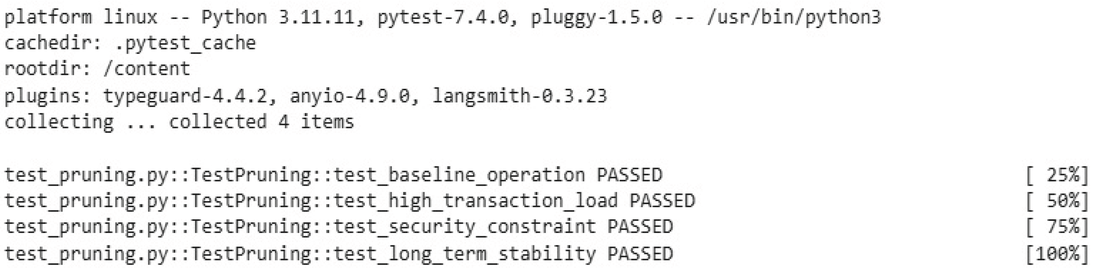
Table A1.
Comparison between IOTA 2.0 and Traditional Blockchain Consensus Mechanisms.
| Metrics | IOTA 2.0 (Mana & FPC) | Blockchain (PoW) | Blockchain (PoS) |
|---|---|---|---|
| Consensus Mechanism | Mana (reputation-based) + FPC (voting-based) | PoW (hash-based) | PoS (stake-based) |
| Energy Consumption | Low | High | Low |
| Storage | Low | High | High |
| Decentralization | High | High | High |
| Scalability | High | Low | Moderate |
| Sybil Protection | Mana | Computational power | Stake |
| Pruning | Local snapshot | Possible | Possible |
Table A2.
Test Cases for IOTA 2.0 Pruning with DQACN.
| Test Case | Description | Parameters | Test Result |
|---|---|---|---|
| Baseline Operation | Run a single edge server with simulated IOTA transactions for 1 hour. | - Storage usage (MB) - Energy usage (CPU %)- Pruning frequency () | Pass |
| High Transaction Load | Simulate 10,000 transactions/hour on 3 edge servers. | - Storage reduction (%) - Energy reduction (%) - Mana value | Pass |
| Security Constraint | Inject 1000 fake transactions; monitor pruning impact. | - Storage for security (MB) - Collision resistance () - Preimage resistance ( 1 & 2) () | Pass |
| Long-Term Stability | Run 5 edge servers for 24 hours with variable transaction rates (1000–5000/hour). | - Storage usage - Energy usage - Agent’s regret (Is it sublinear?) | Pass |
Appendix C.
Table A3.
Simulation Values.
| Notation | Value |
|---|---|
| N | 10-100 |
| 1000-10000 | |
| 0 to 1 | |
| 1000 | |
| 5000 (base) | |
| 5000 × 0.6 = 3000 (base) | |
| 0 to 1000 | |
| 0.9 | |
| 0.1 | |
| 0.4 | |
| 0.4 | |
| 0.2 | |
| 0.05 | |
| Uniform(0.01, 0.1) | |
| 0.0001 |
The pruning decision should be proportional to the mana, i.e. servers receiving more transactions have to prune frequently. The base pruning rate is modeled by the beta distribution in Equation (A22) with the gamma () distribution:
creates the skewed value, leading to the lower pruning rate. The pruning frequency is scaled further with the ratio of finalized messages by FPC and unpruned messages, and normalizing the factor, enabling active servers to prune more. The mana decay in the energy model is as follows. The energy consumption for mana management by server i at time n, accounting for both transaction issuance and decay updates, is given by:
is the number of decay updates, modeled as , with . The Poisson distribution for and is defined by the probability mass function:
The Uniform distribution for is defined by the probability density function:
To handle the network congestion, the transaction rate () of the server is controlled according to its mana value. This is given by below equation.
is the base transaction rate for server i, is the maximum mana across all servers at time n and represents the total network transaction rate at the previous time step . The FPC query rate for server i at time n, scaled by conflict rate, is given by:
is the baseline FPC query rate, is the additional query rate per conflict, is the conflict rate at time n.
Amsterdam Illustration:
We present the example calculation for Amsterdam. For the population of 900,000 ([28]), a 70% smart meter rate ([29]) yields 630,000 smart meters (900,000 × 0.7). Each 50,000 meters requires one edge server ([30]), so there are 630,000 / 50,000 = 12.6 (13) servers. With a rental rate of $5,000 USD per year for an edge server, the baseline rental cost is 13 × $5,000 = $65,000. Without optimization, operational costs become $5,040,000 annually (630,000 × $8/meter, IOTA 2.0), offset savings of $3,780,000 (630,000 × $6/meter, billing efficiency), resulting in a net baseline savings of $3,715,000 ($3,780,000 - $65,000). Algorithm 1, optimizing storage and energy individually, applies a 35% energy reduction and 30% storage reduction (applying lower bound to the solution), increasing savings to $5,475,450 ($3,715,000 × 1.474, reflecting combined energy and storage benefits), a 47.4% gain over the baseline (($5,475,450 - $3,715,000) / $3,715,000 × 100 = 47.4%). Algorithm 2, jointly optimizing pruning frequency, energy, and storage, applies a 40% energy reduction and 35% storage reduction, yielding $5,695,950 ($3,715,000 × 1.534), a 53.4% increase (($5,695,950 - $3,715,000) / $3,715,000 × 100 = 53.4%). Averaging these, the 1-year savings become ($5,475,450 + $5,695,950) / 2 = $5,585,700, reflecting a 50.4% improvement (($5,585,700 - $3,715,000) / $3,715,000 × 100 = 50.4%). This analysis highlights the significant cost efficiency of the cooperative deep Q actor-critic approach, scalable to a 5-year average of $27,928,500 ($5,585,700 × 5), offering substantial benefits for energy providers in smart meter deployments. For the remaining cities, the cost saving for 1 year to 5 years is highlighted in Table 2. From our analysis, it is apparent that energy providers can obtain enormous cost benefits. The cost-benefit is enormously high for highly populated cities like Delhi and Beijing.
Table A4.
Smart Meter Deployment Across Five Cities (as on 2025).
| City | Population | Smart Meters [29] | Edge Servers [30] | Renting Rate |
|---|---|---|---|---|
| Amsterdam | 900,000 [28] | 630,000 | 13 | 5,000 |
| Beijing | 22,000,000 [31] | 15,400,000 | 308 | 5,000 |
| Cincinnati | 300,000 [32] | 210,000 | 5 | 5,000 |
| Delhi | 33,000,000 [33] | 23,100,000 | 462 | 5,000 |
| Milan | 1,400,000 [34] | 980,000 | 20 | 5,000 |
References
- Wan, S.; Lin, H.; Gan, W.; Chen, J.; Yu, P.S. Web3: The Next Internet Revolution. IEEE Internet of Things Journal 2024, 11, 34811–34825. [Google Scholar] [CrossRef]
- Liu, Z.; Xiang, Y.; Shi, J.; Gao, P.; Wang, H.; Xiao, X.; Wen, B.; Li, Q.; Hu, Y.C. Make Web3.0 Connected. IEEE Transactions on Dependable and Secure Computing 2022, 19, 2965–2981. [Google Scholar] [CrossRef]
- Bu, G.; Gürcan, Ö.; Potop-Butucaru, M. G-IOTA: Fair and confidence aware tangle. In Proceedings of the IEEE INFOCOM 2019 - IEEE Conference on Computer Communications Workshops (INFOCOM WKSHPS); 2019; pp. 644–649. [Google Scholar] [CrossRef]
- Guo, F.; Xiao, X.; Hecker, A.; Dustdar, S. Characterizing IOTA Tangle with Empirical Data. In Proceedings of the GLOBECOM 2020 - 2020 IEEE Global Communications Conference; 2020; pp. 1–6. [Google Scholar] [CrossRef]
- Koštál, K.; Bahar, M.N.; Numyalai, S.; Ries, M. Beyond Integration: Advancing Electricity Metering with Secure and Transparent Blockchain-IoT Solutions. In Proceedings of the 2024 47th International Conference on Telecommunications and Signal Processing (TSP); 2024; pp. 324–331. [Google Scholar] [CrossRef]
- Bhavana, G.; Anand, R.; Ramprabhakar, J.; Meena, V.; Jadoun, V.K.; Benedetto, F. Applications of blockchain technology in peer-to-peer energy markets and green hydrogen supply chains: a topical review. Scientific Reports 2024, 14, 21954. [Google Scholar] [CrossRef] [PubMed]
- Tang, W.; Xie, X.; Huang, Y.; Qian, T.; Li, W.; Li, X.; Xu, Z. Exploring the potential of IoT-blockchain integration technology for energy community trading: Opportunities, benefits, and challenges. CSEE Journal of Power and Energy Systems 2025. [Google Scholar]
- Wang, H.; Ma, S.; Guo, C.; Wu, Y.; Dai, H.N.; Wu, D. Blockchain-based power energy trading management. ACM Transactions on Internet Technology (TOIT) 2021, 21, 1–16. [Google Scholar] [CrossRef]
- O’Connor, C.; Collins, J.; Prestwich, S.; Visentin, A. Electricity price forecasting in the irish balancing market. Energy Strategy Reviews 2024, 54, 101436. [Google Scholar] [CrossRef]
- Heo, J.W.; Ramachandran, G.S.; Dorri, A.; Jurdak, R. Blockchain data storage optimisations: a comprehensive survey. ACM Computing Surveys 2024, 56, 1–27. [Google Scholar] [CrossRef]
- Xu, M.; Feng, G.; Ren, Y.; Zhang, X. On cloud storage optimization of blockchain with a clustering-based genetic algorithm. IEEE Internet of Things Journal 2020, 7, 8547–8558. [Google Scholar] [CrossRef]
- Zuo, Y.; Jin, S.; Zhang, S.; Zhang, Y. Blockchain storage and computation offloading for cooperative mobile-edge computing. IEEE Internet of Things Journal 2021, 8, 9084–9098. [Google Scholar] [CrossRef]
- Alofi, A.; Bokhari, M.A.; Bahsoon, R.; Hendley, R. Optimizing the energy consumption of blockchain-based systems using evolutionary algorithms: A new problem formulation. IEEE Transactions on Sustainable Computing 2022, 7, 910–922. [Google Scholar] [CrossRef]
- Akrasi-Mensah, N.K.; Agbemenu, A.S.; Nunoo-Mensah, H.; Tchao, E.T.; Ahmed, A.R.; Keelson, E.; Sikora, A.; Welte, D.; Kponyo, J.J. Adaptive storage optimization scheme for blockchain-IIoT applications using deep reinforcement learning. IEEE Access 2022, 11, 1372–1385. [Google Scholar] [CrossRef]
- Zhou, Y.; Ren, Y.; Xu, M.; Feng, G. An improved nsga-iii algorithm based on deep q-networks for cloud storage optimization of blockchain. IEEE Transactions on Parallel and Distributed Systems 2023, 34, 1406–1419. [Google Scholar] [CrossRef]
- Tanis, Z.; Durusu, A. Cooperative Behaviors and Multienergy Coupling through Distributed Energy Storage in the Peer-to-Peer Market Mechanism. IEEE Access 2025. [Google Scholar] [CrossRef]
- Kreps, D.M. Nash equilibrium. In Game theory; Springer, 1989; pp. 167–177.
- Ma, J.; Zhang, X.; Li, X. Demystifying Blockchain Scalability: Sibling Chains with Minimal Interleaving. In Proceedings of the International Conference on Security and Privacy in Communication Systems. Springer; 2023; pp. 265–286. [Google Scholar]
- Sutton, R.S.; Barto, A.G. Reinforcement Learning: An Introduction, 2nd ed.; MIT Press: Cambridge, MA, 2018. [Google Scholar]
- Bertsekas, D.P.; Tsitsiklis, J.N. Neuro-Dynamic Programming; Athena Scientific: Belmont, MA, 1996. [Google Scholar]
- Tsitsiklis, J.N. Asynchronous Stochastic Approximation and Q-Learning. Machine Learning 1994, 16, 185–202. [Google Scholar] [CrossRef]
- Konda, V.R.; Tsitsiklis, J.N. Actor-Critic Algorithms. SIAM Journal on Control and Optimization 2000, 42, 1143–1166. [Google Scholar] [CrossRef]
- Sutton, R.S.; McAllester, D.A.; Singh, S.P.; Mansour, Y. Policy Gradient Methods for Reinforcement Learning with Function Approximation. In Proceedings of the Advances in Neural Information Processing Systems 12 (NIPS 1999); Solla, S.A.; Leen, T.K.; Müller, K.R., Eds. MIT Press; 2000; pp. 1057–1063. [Google Scholar]
- Tsitsiklis, J.N.; Van Roy, B. An Analysis of Temporal-Difference Learning with Function Approximation. IEEE Transactions on Automatic Control 1997, 42, 674–690. [Google Scholar] [CrossRef]
- Kakade, S. A Natural Policy Gradient. In Proceedings of the Advances in Neural Information Processing Systems 14 (NIPS 2001); Dietterich, T.G.; Becker, S.; Ghahramani, Z., Eds. MIT Press; 2002; pp. 1531–1538. [Google Scholar]
- Williams, R.J. Simple Statistical Gradient-Following Algorithms for Connectionist Reinforcement Learning. Machine Learning 1993, 8, 229–256. [Google Scholar] [CrossRef]
- Filar, J.; Vrieze, K. Competitive Markov Decision Processes; Springer: New York, NY, 1997. [Google Scholar] [CrossRef]
- UN Population Division. World Urbanization Prospects, 2018. 2018 Revision.
- International Energy Agency. Smart Meters in Buildings, 2023.
- AWS IoT Architecture Guidelines, 2023.
- National Bureau of Statistics of China. China Statistical Yearbook, 2023.
- U.S. Census Bureau. American Community Survey, 2023. 2023 Estimates.
- UN Data. India Population Projections, 2023.
- Eurostat. Urban Population Statistics, 2023.
Figure 1.
Overall Architecture.
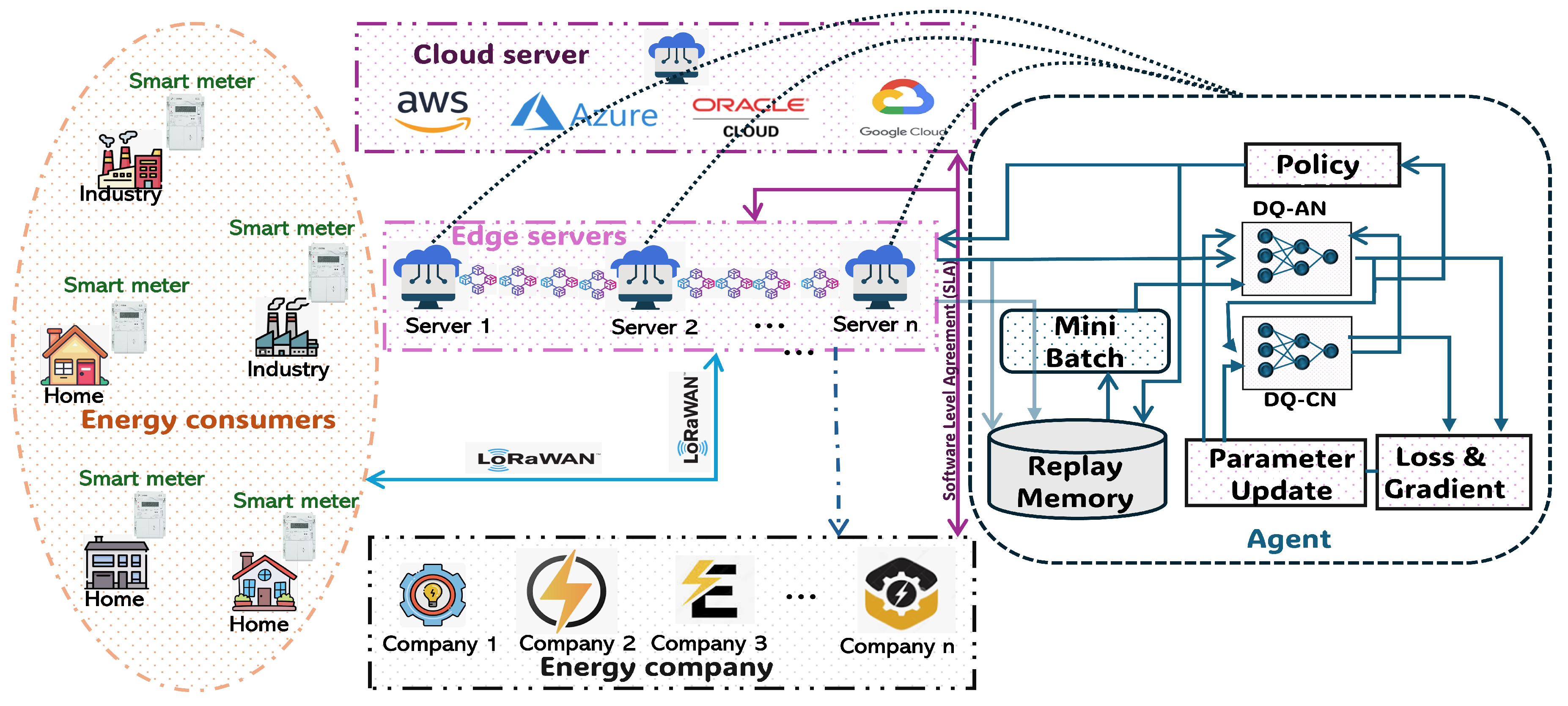
Figure 2.
Issues in Local Snapshot.
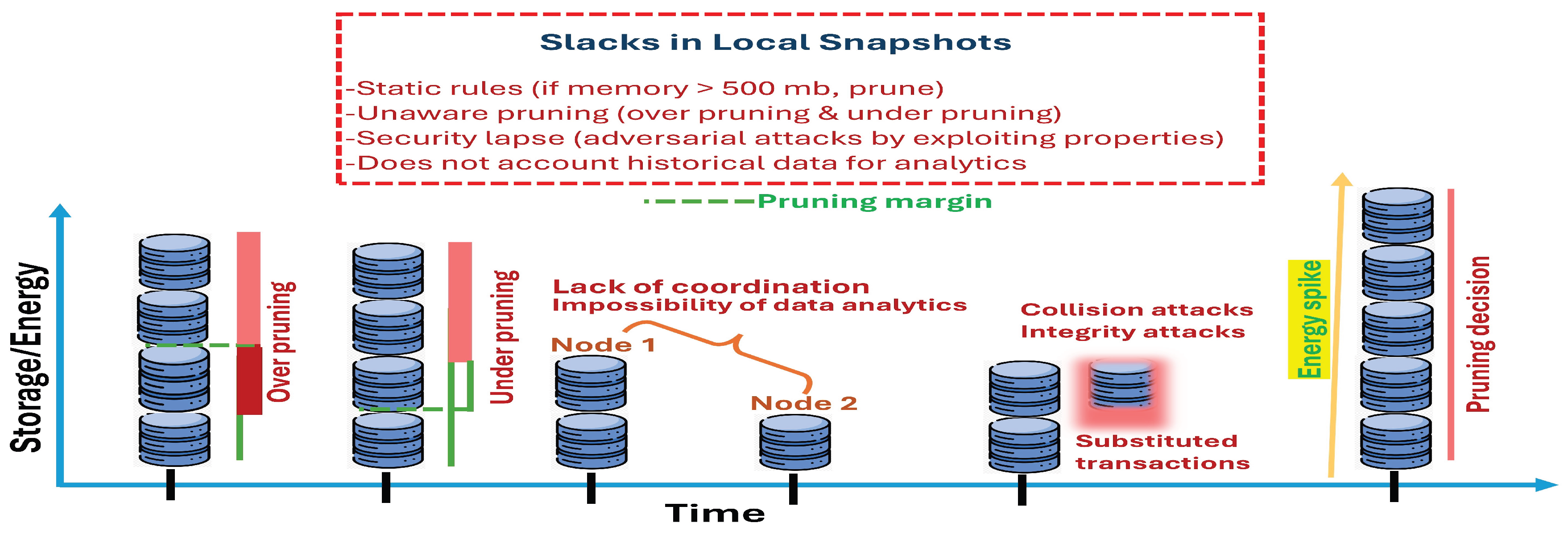
Figure 3.
Deep Q Actor-Critic Network Architecture with Method.
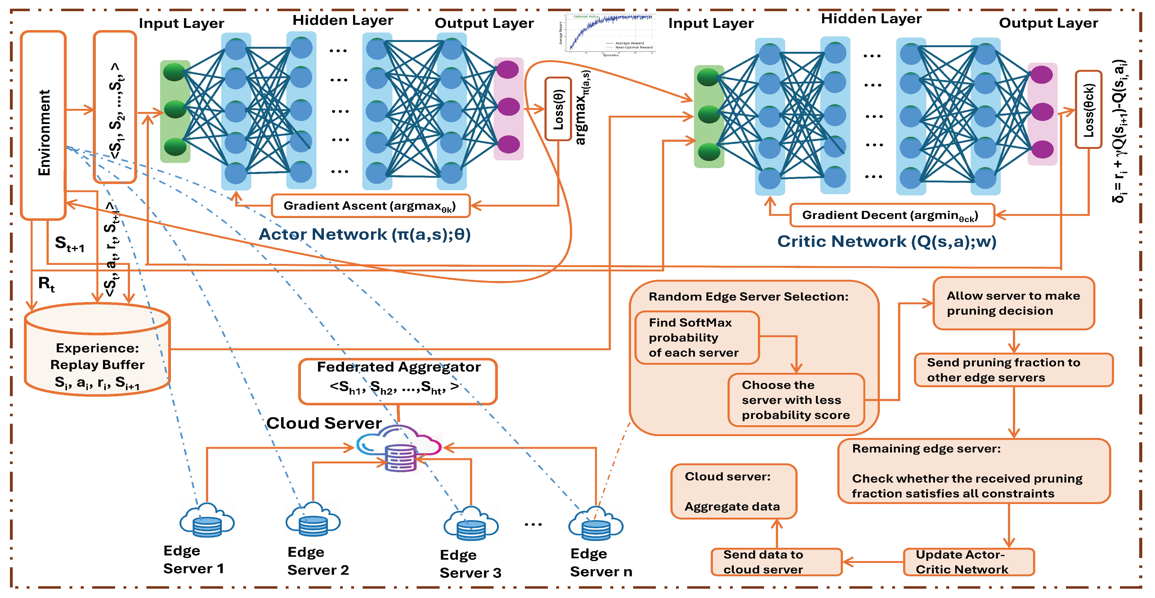
Figure 4.
Simulation Result: Edge servers Vs Total Cost (1), Storage Cost (2), Energy Cost (3) and Pruning Frequency (4), Transactions Vs Total Cost (5), Storage Cost (6), Energy Cost (7) and Pruning Frequency (8), Pruning Frequency Vs Total Cost (9), Storage Cost (10), Energy Cost (11) and Constraints Satisfaction (12).
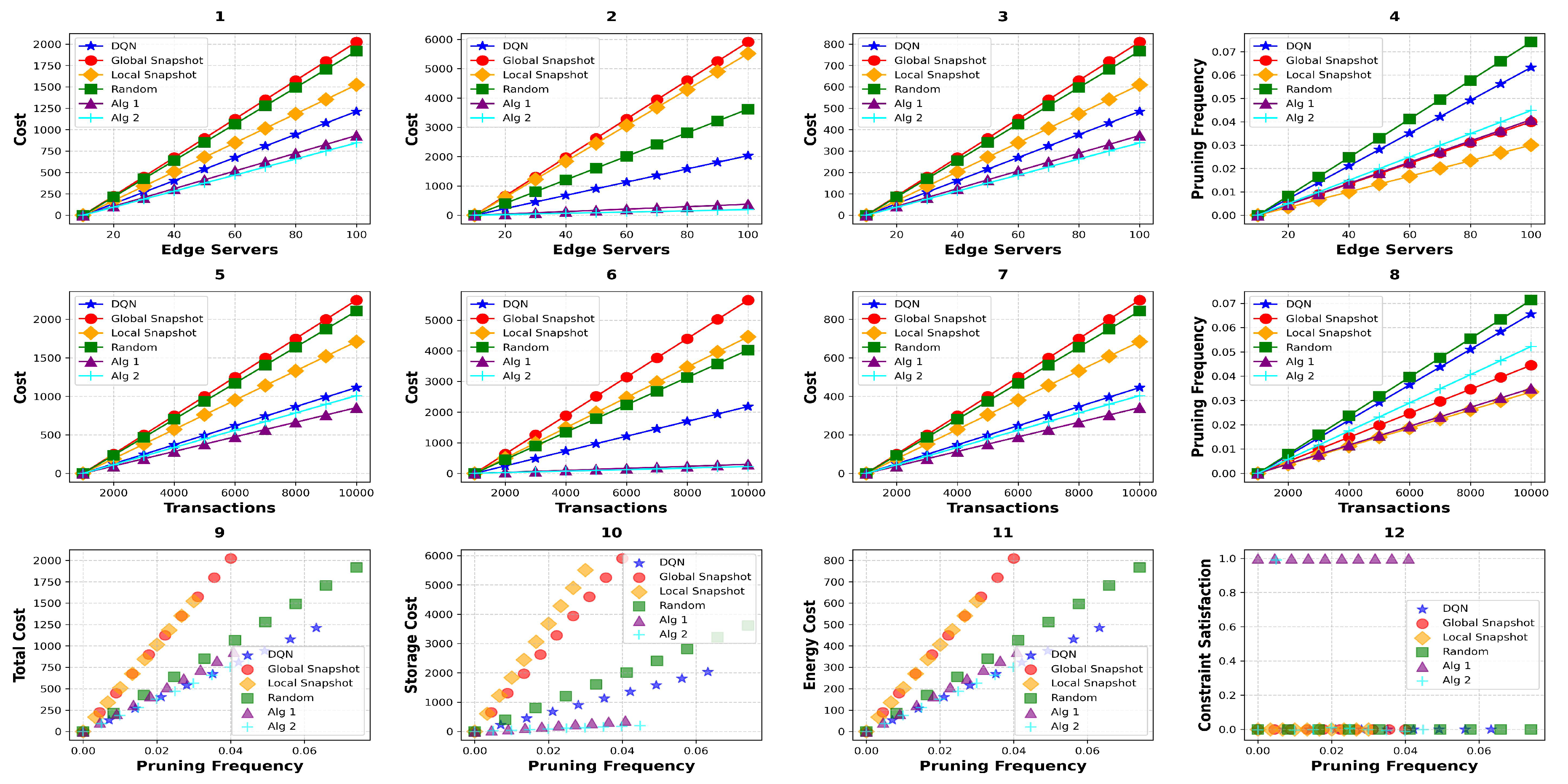
Table 1.
Nomenclature.
| Notation | Description |
|---|---|
| Generic Variables | |
| N | Total number of edge servers |
| n | Time |
| Subset of edge servers participating in FPC consensus at time n | |
| Energy cost per hash computation | |
| Energy cost per signature computation | |
| Energy cost per pruning operation | |
| Energy cost per FPC query/vote operation at server i | |
| Energy cost per mana update operation at server i | |
| Energy cost per message attachment operation at server i | |
| Efficiency factor of server i | |
| Mana of server i at time n | |
| Nodes involved in the consensus (binary variable) | |
| Mana decay rate | |
| Mana scaling factor | |
| Set of smart meters pledging mana to server i | |
| Message Variables | |
| Number of messages processed by server i at time n | |
| Number of hash computations per message at server i | |
| Number of signature verifications per message at server i | |
| Number of FPC queries/votes by server i at time n | |
| Number of mana updates due to message issuance by server i at time n | |
| Number of mana decay updates by server i at time n | |
| Pruning Variables | |
| Fraction of messages pruned by server i at time n | |
| Total unpruned messages at server i at time n | |
| Number of finalized messages at server i at time n | |
Disclaimer/Publisher’s Note: The statements, opinions and data contained in all publications are solely those of the individual author(s) and contributor(s) and not of MDPI and/or the editor(s). MDPI and/or the editor(s) disclaim responsibility for any injury to people or property resulting from any ideas, methods, instructions or products referred to in the content. |
© 2025 by the authors. Licensee MDPI, Basel, Switzerland. This article is an open access article distributed under the terms and conditions of the Creative Commons Attribution (CC BY) license (http://creativecommons.org/licenses/by/4.0/).
Copyright: This open access article is published under a Creative Commons CC BY 4.0 license, which permit the free download, distribution, and reuse, provided that the author and preprint are cited in any reuse.


