
Submitted:
05 August 2025
Posted:
06 August 2025
You are already at the latest version
Abstract
Mathematical modeling is indispensable in oncology for unraveling the complex interplay between tumor growth, vascular remodeling, and therapeutic resistance. Here, we address the critical need for integrative frameworks capturing bidirectional feedback between hypoxia-driven angiogenesis and stochastic resistance evolution, an aspect often treated in isolation by previous continuum or agent-based models. We develop a novel hybrid partial differential equation–agent-based model (PDE-ABM) formulation unifying reaction-diffusion equations for oxygen, drug, and tumor angiogenic factor (TAF) with Gillespie-driven stochastic phenotype switching and discrete vessel-agent dynamics. Our work fills a methodological gap by providing the first rigorous well-posedness proof for this class of coupled systems, alongside detailed numerical analysis of discretization schemes and derivation of analytically tractable mean-field PDE limits via moment-closure techniques. The mean-field limit unifies the hybrid system into one PDE system, linking stochastic microdynamics with deterministic macrodynamics. By combining mathematical rigor with biologically interpretable outputs, our framework establishes a foundation for predictive multiscale oncology models and enables future data-driven therapeutic design.
Keywords:
mathematical oncology
; tumor resistance
; angiogenesis
; hypoxia
; hybrid and multiscale modeling
; reaction-diffusion equations
; agent-based model
; mean-field limit
; stochastic phenotypic switching
1. Introduction
Cancer remains a leading cause of global mortality, accounting for 16.8% of all deaths and 22.8% of noncommunicable diseases-related deaths [1]. Despite advances in targeted therapy, immunotherapy, and radiotherapy, therapeutic resistance persists as the primary barrier to achieving durable cures, often resulting in relapse or refractory disease [2]. Here, we focus on how resistance mechanisms—particularly those driven by tumor angiogenesis—undermine current treatments and perpetuate poor prognosis. Resistance arises from both intrinsic tumor heterogeneity (e.g., spatial and temporal genetic diversity [3]) and adaptive responses to therapy, with the tumor microenvironment (TME) playing a pivotal role. Among these factors, dysregulated angiogenesis emerges as a critical facilitator of resistance. Tumors hijack pro-angiogenic pathways (e.g., vascular endothelial growth factor/vascular endothelial growth factor receptor (VEGF/VEGFR), hypoxia-inducible factor 1 (HIF-1)) to sustain growth, while suppressing anti-angiogenic signals (e.g., thrombospondin-1 (TSP-1)) [4]. This "angiogenic switch" not only fuels tumor progression but also establishes a resilient vascular niche that evades therapy. Although anti-angiogenic agents (e.g., bevacizumab) initially improve progression-free survival by blocking VEGF, their long-term efficacy is limited by rapid resistance [5,6]. Critically, tumors activate compensatory pathways (e.g., fibroblast growth factor 2 (FGF-2), Interleukin-8 (IL-8), and Angiopoietin-2 (ANGPT-2)) to restore angiogenesis [7], while stromal components (e.g., tumor-associated macrophages (TAMs), myeloid-derived suppressor cells (MDSCs)) further sustain vascular remodeling via cytokine secretion [8]. These findings reveal a paradox: angiogenesis inhibition may inadvertently select for more aggressive, adaptive phenotypes. To overcome this challenge, we argue that disrupting the dynamic crosstalk between tumor cells and the angiogenic TME is essential. Recent studies suggest that combinatorial targeting of both VEGF and compensatory pathways (e.g., FGF-2/IL-8) may delay resistance [9]. However, a systematic framework to predict tumor adaptive responses and optimize combination regimens is still lacking. In this study, we propose a computational hybrid model to identify vulnerabilities in angiogenic networks and investigate the bidirectional coupling between angiogenesis and tumor resistance evolution. To address this need, we first contextualize existing modeling paradigms that inform such integrative frameworks.
Continuum models efficiently capture bulk tumor growth and transient dynamics. The Keller-Segel framework describes cell migration via partial differential equations (PDEs), where endothelial cells follow chemical gradients [10]. Such models assume continuous cell densities, overlooking individual cell heterogeneity. The Fisher-KPP equation [11,12] links proliferation and motility to model tumor spread as reaction-diffusion waves, but cannot resolve rare stochastic events like resistance mutations. Discrete models track individual cell behaviors and microenvironment heterogeneity. Anderson et al. [13] pioneered agent-based models (ABMs) to simulate capillary sprouting through stochastic tip-cell migration rules, but lack coupling to continuum metabolite fields (e.g., oxygen gradients) and microenvironmental feedback (e.g., hypoxia-driven angiogenesis). Despite these advances, both approaches face inherent limitations: Continuum models lack single-cell resolution for stochastic events (e.g., mutations, phenotype switching) and spatiotemporal heterogeneity, while discrete models are computationally prohibitive for large-scale dynamics (e.g., diffusion, fluid flow). This dichotomy motivates hybrid frameworks that transcend scale constraints.
Hybrid discrete-continuum (HDC) models integrate agent-based rules with reaction-diffusion equations to reflect cancer’s multiscale nature [14,15,16]. Some hybrid models address drug resistance evolution. Gevertz et al. [17] coupled continuous drug and oxygen fields with agent-based tumor dynamics to study preexisting and acquired resistance, but assumed stationary vessels, uniform resistance acquisition capacity, and continuous drug administration. Picco et al. [18] modeled environmentally mediated drug resistance (EMDR) using drug and signaling fields, generating EMDR by increasing vascular density but neglecting vascular remodeling. Other hybrid models coupled tumor growth with angiogenesis [19,20]. Macklin et al. [21] developed a multiscale framework integrating extracellular matrix, angiogenesis, and tumor progression. Despite these innovations, a critical gap persists: Most models simulate vascular remodeling or resistance in isolation, omitting spatiotemporal feedback where vessel adaptation alters resistance trajectories. One exception is Wang et al. [22], which proposed a hybrid model coupling hypoxia-induced angiogenesis with resistance selection, but left unresolved three limitations: (i) inadequate mathematical analysis of the hybrid system, insufficient numerical scheme analysis, and absence of derived mean-field limits for agent dynamics. Our work directly addresses these gaps while extending their framework.
We advance the hybrid paradigm in [22] through three innovations: First, we introduced a spatially resolved model unifying stochastic phenotypic switching via a Gillespie algorithm to capture drug-induced resistance transitions. Second, we incorporate metabolite-regulated angiogenesis where vessel agents respond to dynamic hypoxia (o) and tumor angiogenic factor (TAF) (c) gradients. Third, we establish bidirectional coupling enabling emergent feedback between hypoxia, angiogenesis, and resistance evolution. Consequently, this framework yields three contributions: rigorous mathematical analysis of the coupled PDE-ABM system and numerical analysis of PDE discretization schemes; integration of exact stochastic resistance (Gillespie ABM) with physics-driven angiogenesis (PDE-coupled ABM); and derivation of analytically tractable continuum mean-field limits from discrete rules. The mean-field limit integrates the hybrid system into one PDE system, linking stochastic microdynamics with deterministic macrodynamics. It motivates innovative hybrid numerical schemes that selectively retain the full ABM structure in critical regions while replacing it with efficient PDE surrogates elsewhere. By unifying PDE analysis, stochastic analysis, and numerical analysis, our framework moves beyond descriptive modeling to establish rigorous mathematical foundations for hybrid PDE-ABM systems.
The paper is structured as follows: Section 2 details the hybrid formulation. Section 3 links our model to classical mathematical biology frameworks and outlines contributions. Section 4 provides mathematical analysis of the coupled system. Section 5 presents numerical analysis, including consistency, stability, convergence, and conservation properties. Section 6 concludes.
2. Material & Methods
Building on the Introduction’s biological foundations, we formalize a hybrid PDE-ABM with bidirectional coupling between continuum fields (TAF, drug, oxygen) and discrete agents (tumor and vessel cells). Reaction-diffusion equations govern TAF (c), drug (d), and oxygen (o) dynamics. Endothelial cell (n) migration follows increasing TAF concentrations via the chemotaxis equation:
Discrete tumor and vessel agents interact with the TME through stochastic rule-based ABM dynamics. We denote tumor, normoxic, hypoxic, tip, and vessel agent sets at time t as , , , , and , respectively. Local oxygen levels partition the tumor population into normoxic () and hypoxic () subpopulations. Full model details appear in [22]. We present the non-dimensionalized system for ; the original dimensional system and non-dimensionalization procedure derive from Appendix A.
Here, , , , are diffusion coefficients; is the chemotactic sensitivity; is the saturation parameter; , , are decay rates; , are cellular uptake rates; , are supply rates from blood vessels; and , are production/uptake rates of TAF. , are characteristic functions that equal 1 within disks of cellular radius :
Here, denote the position center of a and v. We choose a closed domain with boundary and impose homogeneous Neumann conditions:
where is the outward unit normal at .
Tumor and vessel agents evolve on a lattice discretizing the ABM domain into squares of side length . Tip cell motion uses the Von Neumann neighborhood structure (four orthogonal neighbors), while agent-microenvironment interactions use the Moore structure (eight neighbors including diagonals).
We construct a PDE domain with boundary approximating . Appendix B details the mapping and the numerical derivation of the discrete lattice in the ABM. Briefly, define the open -neighborhood of with . Convolve its characteristic with a compactly supported mollifier , and set
for small ensuring . This yields a domain whose boundary is proximal to . We obtain the discrete approximation by sampling on the ABM lattice, thresholding at level , and identifying boundary agents as those with Moore neighbors outside . Algorithm A1 summarizes the construction.
Each tumor cell has state:
denoting position, local oxygen, accumulated drug, DNA damage, death threshold, age, and maturation time. Each tip cell b has state:
for position and age since the last branching. Agent states update via Markov processes under the time discretization of :
where is the Markov transition operator [22]. Algorithm A2 summarizes the transition operator for each mark x. for tumor and endothelial tip cells. Local cell density includes tumor-vessel interactions in our current model:
We decouple phenotype switching from cell division. Unlike classical mutation models linking resistance acquisition to division events, stochastic transitions occur through continuous-time Markov processes independent of division cycles. Mutation elevates the death threshold, DNA repair rate, and oxygen consumption rate but reduces the proliferation rate. Phenotypic traits
take sensitive () and resistant () values:
Cells stochastically switch between these states according to the reaction channels
where baseline rates and , drug sensitivity coefficients and , sensitive-to-resistant mutation rate and resistant-to-sensitive mutation rate
govern phenotypic switching. Each tumor cell bears a phenotypic mark , updated independently of the cell cycle via the Gillespie algorithm [23]. Waiting times follow an exponential distribution with mean (: total propensity):
| Algorithm 1 Stochastic phenotype switching via the Gillespie Direct Method |
|
Each switching event selects the reacting agent by propensities, flips its phenotype (), and updates time-dependent quantities. Algorithm 1 encapsulates phenotype switching procedures. This Gillespie framework permits resistance emergence independent of cell division, capturing stochastic gene expression fluctuations. It thus recovers resistance in rare subpopulations that deterministic ordinary differential equation (ODE)/PDE models average out, and naturally quantifies treatment schedule effects on resistance probability and timing. Table 1 summarizes all parameters in our hybrid PDE-ABM, categorized by continuum PDEs, discrete ABM rules, and numerical implementation.
Our model uniquely captures bidirectional feedback: how hypoxia induces angiogenesis, which alters drug delivery and selects for resistance. The theoretical framework justifies how small changes in local oxygen or vessel density can produce nonlinear shifts in resistance trajectories. These feedback mechanisms align with clinical observations where anti-angiogenic therapies may paradoxically increase resistance risk. Thus, the model could be used to explore: (i) critical thresholds in vessel remodeling that shift tumor response from chemosensitive to chemoresistant, and (ii) timing effects, e.g., whether anti-angiogenic pre-treatment amplifies or delays resistant onset.
3. Connection to Classical Mathematical Biology Frameworks and Contributions
Having formalized our multiscale framework, we contextualize its biological relevance through its mathematical lineage. This section demonstrates that limiting cases of our hybrid PDE-ABM system reduce rigorously to three foundational frameworks: Keller-Segel chemotaxis, Fisher-KPP invasion waves, and Galton-Watson branching processes. These connections are mathematically exact. For a small chemokine concentration c such that , the endothelial cell equation simplifies to the classical Keller-Segel form:
Our model generalizes Keller-Segel by incorporating nonlinear chemotactic saturation and ABM coupling.
While endothelial migration follows chemotactic principles, tumor proliferation exhibits distinct spatiotemporal dynamics. This divergence aligns with the Fisher-KPP paradigm, governed by the equation:
where denotes density, D diffusion, growth rate, and K carrying capacity. Under normoxic conditions () and negligible drug (), tumor density equation (Equation (4.5) reduces to
This predicts traveling wavefronts with minimal speed . Crucially, our full model extends this framework by incorporating microenvironmental heterogeneity (oxygen gradients, drug distribution), which distorts wavefronts into clinically observed asymmetric invasion patterns.
Complementing continuum-scale dynamics, cellular-scale proliferation exhibits stochastic foundations. Absent spatial coupling and microenvironmental feedback (e.g., well-mixed conditions), tumor lineage expansion follows a Galton-Watson branching process. A normoxic cell divides with probability or dies with probability in time interval . yielding the offspring distribution:
For two phenotypes (drug-sensitive S, drug-resistant R), this extends to a two-type Galton-Watson process with expected offspring matrix:
Crucially, classical branching models restrict phenotypic switching to division events. In contrast, our framework implements phenotype switching via a continuous-time Markov process simulated using the Gillespie algorithm (Algorithm 1), enabling asynchronous phenotype evolution independent of the cell cycle. Figure 1 illustrates interactions between branching proliferation and stochastic phenotype switching.
Our mathematically rigorous, biologically grounded HDC framework extends classical theories through multiscale feedback, stochastic switching, and microenvironmental coupling. It advances hybrid modeling by integrating agent-based stochastic phenotypic switching, continuum reaction-diffusion metabolite fields, and bidirectional vascular-resistance coupling. We provide analytical guarantees for model well-posedness, numerical robustness, and mean-field limits. Our contributions distinguish themselves from existing oncology hybrid models (e.g., [39,40,41]) in four key aspects:
- (i)
- Mean-Field Limits: Unlike direct continuum PDE-ABM coupling or variance reduction methods [39,40], we prove convergence from the stochastic agent-based description to a deterministic PDE limit using chemical master equations (CMEs) and moment closures. This yields a unified continuum system (4.6), linking stochastic microdynamics to deterministic macrodynamics. It motivates innovative hybrid numerical schemes retaining ABM structures in critical regions while employing efficient PDE surrogates elsewhere.
- (ii)
- Well-Posedness Analysis: While most stochastic-hybrid models prioritize computation over analytical soundness [40,41], we establish complete well-posedness for our hybrid PDE-ABM system. This includes the existence, uniqueness, and regularity of weak solutions (Theorems 1-3), plus analysis of numerical schemes: consistency (Section 5.2), conditional stability (Theorem 6), convergence (Theorem 7), nonnegativity (Theorem 8) and mass conservation (Theorem 9).
- (iii)
- Stochastic-Deterministic Feedback: Unlike [39], who model virus spread in lung tissue, our hybrid system couples cell phenotype switching, angiogenic fields, and vascular remodeling. This reveals nonlinear resistance dynamics driven by environment-phenotype feedback, underpinned by rigorous mathematics and mean-field approximations.
- (iv)
- Clinical interpretability: While stochastic interacting particle fields (SIPFs) [41] or variance reduction techniques [40] emphasize algorithmic efficiency, our model explicitly links parameters (e.g., mutation rates, oxygen thresholds, drug uptake) to clinical outcomes (e.g., tumor front speed, resistance emergence). This offers a framework for optimizing treatment timing and dosage.
Thus, our work uniquely combines mathematical rigor (well-posedness, mean-field limits) with biologically interpretable hybrid modeling, delivering methodological novelty and translational potential beyond current stochastic-hybrid cancer models.
4. Mathematical Analysis of the Coupled PDE-ABM System & Results
Biological motivation supports the hybrid model design, but rigorous mathematical analysis remains essential to establish its validity and predictive reliability. This section systematically investigates the coupled PDE-ABM framework through three analytical pillars: (i) well-posedness of the PDE-ABM system (Section 4.1), guaranteeing solution existence, uniqueness, and regularity; (ii) master equation and mean-field analysis (Section 4.2), connecting discrete stochastic dynamics to deterministic continuum-scale approximations; and (iii) validity regimes for moment closure approximations, linking microscopic randomness with macroscopic behavior. This triad ensures mathematical robustness for therapeutic applications, including chemotherapy optimization and anti-angiogenic interventions.
4.1. Well-Posedness
We establish existence, uniqueness, and regularity of weak solutions for the coupled PDE-ABM system governing the continuous fields . Without agent interactions, the PDEs reduce to a classical linear parabolic system with guaranteed well-posedness. We formalize this foundation using the Lions–Gelfand triple framework [Theorem 10.9 [42]; see [43] for detailed proofs.
Lemma 1
(J.-L. Lions). Let be a Gelfand triple, with V and H Hilbert spaces and V densely and continuously embedded into H. The scalar product and norm for H are and , and the norm for V is . Let . Suppose for almost every , is a time-dependent bilinear form satisfying:
- (i)
- For all , the function is measurable.
- (ii)
- for almost every and all .
- (iii)
- for almost every and all .
where , M, and C are constants. Then for and , there exists a unique function
satisfying the weak formulation:
with initial condition .
We now apply this result to the coupled reaction-diffusion equations on the finite time interval :
where and incorporates agent-dependent reaction terms:
We omit the analysis of the endothelial density equation:
Classical two-dimensional Keller–Segel systems exhibit chemotactic blow-up, that is, unbounded density in finite time [44,45], but admit global solutions under small-mass conditions. In particular, consider the following parabolic-elliptic Keller-Segel system:
where is the outward unit normal to and denotes the spatial average of n. Assume the initial mass satisfies:
Then, a global-in-time weak solution exists under the following conditions:
- (i)
- Bounded domain case: If U is a bounded, connected domain and ,
- (ii)
- Whole space case: If , with and .
Discrete agents represent the endothelial population in our hybrid formulation, replacing continuous density and further regularizing dynamics. Each tip occupies at most one lattice site. Vessel elongation occurs with a fixed period , and branching requires the tip cell age to exceed the threshold (). Anastomosis stabilizes the system: tip encounters cause emerging, reducing the tip count. These rules ensure a finite agent population and prevent uncontrolled mass concentration, consistent with lattice-based chemotaxis ABMs [13,28,47,48]. We thus focus our analysis on the subsystem. To manage PDE-ABM coupling, we introduce:
Assumption A1
(PDE-ABM Coupling).
- (i)
- The spatial domain is bounded with boundary .
- (ii)
- The initial data is nonnegative and belongs to .
- (iii)
- For all and lattice sites :
Assumption A1 (iii) imposes a uniform local density bound, not global agent boundedness, as tumor proliferation may increase over time. This aligns with the biological crowding constraint in ABM rules: lattice sites accommodate finitely many agents within radius , and cell division halts at local density . Consequently, global agent growth does not compromise the local boundedness of PDE source terms, which is essential for coupled system well-posedness.
We define the weak formulation by seeking satisfying and for each , with:
and initial conditions . Here denotes the inner product, and is the duality pairing.
Theorem 1
(Existence and Uniqueness of Weak Solutions). Assumption A1 guarantees unique weak solutions for the coupled PDE-ABM system (4.1) with:
Proof.
Apply Lemma 1 to each component via the Gelfand triple and coercive, bounded bilinear forms for . □
We rigorously couple ABM and PDE dynamics through time discretization and operator splitting:
Theorem 2
(Well-posedness of the Coupled PDE-ABM System). Under Assumption A1 on with time steps :
- (i)
- The PDE subsystem admits a unique weak solution with Theorem 1 regularity.
- (ii)
- The ABM subsystem defines càdlàg Markov process almost surely for agent marks
Proof.
Use mathematical induction over intervals . For , Theorem 1 establishes existence, uniqueness, and regularity on with initial data and fixed agent . Assume the result holds on . For :
- (i)
- Solve the parabolic subsystem on :which has unique weak solutions by Theorem 1.
- (ii)
- Evolve ABM marks on via:where is the Markov transition operator. Piecewise constant agent trajectories with right-continuous and left limits ensure the càdlàg Markov property.
Induction extends the result to . □
Remark 1
(Justification of Stepwise Decoupling). Theorem 2 solves the PDE subsystem on each interval with fixed agent configuration . This approach directly implements the hybrid model’s operator–splitting scheme: PDE fields evolve continuously via (4.3) on . While agent updates occur discretely at . Consequently, PDE source terms are piecewise constant in time, preserving well-posedness as a linear parabolic problem on each subinterval. The ABM update (2.2) defines a Markov map at mesh points.
Since the alternating-update rule defines the hybrid model itself, no splitting error accumulates. The piecewise-constant ABM forcing is an exact model component. The induction argument formalizes this sequential construction, guaranteeing existence and uniqueness on each and hence on .
We examine the decoupled system to highlight the ABM’s role. The resulting linear parabolic PDEs with Neumann boundary conditions admit a classical solution via spectral decomposition of the Neumann Laplacian (proof in [49]):
Theorem 3
(Well-Posedness of Sole PDE System). The system
admits a unique classical solution:
where the Neumann Laplacian eigenbasis satisfies:
with eigenvalues . Coefficients are . Each is spatially smooth for and temporally analytic for .
The spectral result confirms that without ABM interactions, the PDE subsystem maintains full regularity and decouples completely. In the coupled system, agent density constraints ensure well-posedness despite nonlinear agent-driven reaction terms. Thus, our hybrid framework is both analytically well-posed and biologically interpretable, providing a solid foundation for clinical applications.
Weak solution existence establishes a rigorous mathematical foundation for hybrid models integrating microscopic interactions with macroscopic behaviors. The proof of well-posedness for the coupled PDE-ABM system guarantees that the model behaves predictably under biologically relevant conditions, e.g., bounded agent density due to cell crowding and realistic spatial constraints. This is critical for ensuring that simulated phenomena like angiogenesis, hypoxia-driven resistance, and spatial tumor heterogeneity reflect biological processes rather than numerical artifacts. From a clinical perspective, this mathematical well-posedness lays the foundation for future optimization of treatment regimens (e.g., dosing schedules) within a consistent modeling framework.
4.2. Master Equation Formulation and Mean-Field Limit
Having established deterministic well-posedness, we now analyze stochastic aspects of agent dynamics. Integrating stochastic agent-based dynamics within a continuum PDE framework requires principled linkages between microscopic randomness and macroscopic observables. The CME provides this foundation by capturing the probabilistic evolution of the agent state space. This section derives a lattice-based CME for the hybrid PDE-ABM system, computes first-order moment equations, and establishes conditions justifying a deterministic mean-field approximation. By unifying the hybrid PDE-ABM into a continuous description (4.6), our model connects microscale interactions with macroscale dynamics, replacing the computationally demanding ABM structure in dense tumor regions with an efficient PDE solver.
We analyze a coarse-grained mesoscopic representation of the ABM component. Consider a regular lattice with spacing over the spatial domain. The local agent density function denotes the tumor agent count at site and time t.
Let represent the discrete ABM configuration at time t. A continuous-time Markov process on governs the stochastic evolution of , with state-dependent transition rates determined by agent rules, including proliferation, death, motility, and phenotypic switching.
Let denote the probability mass function over all ABM configurations. The CME governing the evolution of is:
where denotes the transition rate from configuration to . Each transition corresponds to elementary stochastic events with specific forms:
- (i)
- Brownian Movement: each cell jumps to neighboring site at ratewhere denotes the Von Neumann neighborhood (four orthogonal neighbors) of . The coefficient originates from the Fokker-Planck equation for tumor agents undergoing Brownian motion: with independent standard Brownian motions.
- (ii)
- Regulated Proliferation: Using the Heaviside function H to identify normoxic states, only normoxic cells proliferate at rate
- (iii)
- Drug-Induced Death: Apoptosis occurs at constant rate : .
- (iv)
- Mutation: mutation preserves cell counts per voxel, and thus does not appear in the CME.
Define the expected local agent density:
The cádlág property yields:
The CME governs the change rate due to proliferation, death, and movement:
This equation is unclosed because first-order moments depend on higher-order correlations through nonlinear functions. A tractable macroscopic approximation requires closure. The mean-field approximation assumes statistical independence between agent states, providing the first-moment closure:
Applying this closure yields:
Define the density gives , producing the CME for :
The deterministic approximation holds under the law of large numbers when local agent populations are large and suppress fluctuations. The continuum limit yields the macroscopic density equation:
where . In the continuum limit, the local cell count is
where and denote tumor and vessel agent spatial densities. The uniform bound implies the tumor cell density constraint:
where begin the disk area. The maximum local cell count follows as
thus .
Therefore, applying first-order moment closure yields a deterministic approximation of the tumor density dynamics. This closure is valid under large-population and weak-correlation regimes.
Theorem 4
(Mean–Field Limit for the Tumor Cell Density). Let denote tumor cell agent counts evolving under the stochastic rules in Section 2 on a lattice with spacing . Assume:
- (i)
- Initial agent positions and states are i.i.d. with macroscopic density .
- (ii)
-
The maximum local occupancy satisfieswhere is the maximal local cell–vessel occupancy value and the cell radius.
Then, as and , the tumor cell density satisfies:
Here is the macroscopic carrying capacity, H the Heaviside function, the positive part, and d the drug concentration. Diffusion arises from cellular Brownian motion; the reaction term models normoxic proliferation and drug-induced apoptosis.
Theorem 4 provides the leading–order deterministic approximation via first–order moment closure. Agent-based simulations are computationally intensive for tumor populations. The mean-field limit unifies the hybrid model into a computationally efficient continuum description:
The mean-field equation (4.6) allows one to interpret complex, stochastic agent-based behavior through simpler, deterministic PDEs. This bridge from microscale (single-cell events like stochastic phenotype switching) to macroscale (tumor cell density evolution) enables: (i) analytical estimation of tumor front velocity, aiding prognosis (e.g., time to vascular invasion or metastatic risk), (ii) sensitivity to environmental factors (e.g., hypoxia, drug gradients) to be encoded directly in continuous equations, which may inform spatially-resolved treatment planning, and (iii) approximate solutions in real time, supporting integration into clinical decision-support tools, where full ABM simulations may be computationally prohibitive. On the other hand, mean-field approximations neglect fluctuations, so we clarify valid parameter regimes and biological relevance.
Remark 2
(Validity Regime of the Moment Closure). Equation (4.5) uses first–order moment closure , neglecting second-order moments and higher–order cumulants. This requires:
- (i)
- Large local populations: per site , making demographic noise under central limit scalings;
- (ii)
- Weak correlations:Negligible spatial correlations between neighboring voxels at scale , ensured by fast mixing (large ε) or weakly interactions.
Fluctuations then contribute only corrections, so (4.5) captures population dynamics to leading order.
Biologically, these hold in dense tumor regions where local interactions average stochasticity. They fail in:
- (i)
- Early growth stages, invasion fronts, or metastatic niches with small and non-negligible extinction;
- (ii)
- Strongly heterogeneous microenvironments where correlations and clustering invalidate the weak–fluctuation assumption.
Solutions include second-order moment closure (e.g., pair approximations) or hybrid models retaining ABM structures in critical regions while using PDE surrogates elsewhere. These are active multiscale modeling research areas.
5. Numerical Analysis & Results
We rigorously evaluate the numerical properties of the hybrid PDE-ABM scheme. First, we detail the discretization framework for both continuous and agent-based components. We then analyze consistency, stability, and convergence, verifying critical biological features including nonnegativity and mass conservation. Finally, we validate theoretical convergence through grid refinement tests.
5.1. Hybrid Time-Stepping Framework
We discretize a square computational domain of area using a uniform Cartesian grid with m, yielding a mesh. We evolve TAF, drug, and oxygen fields via a semi-implicit alternating direction implicit (ADI) scheme, updating reaction terms explicitly. Endothelial cell density advances using an explicit forward Euler method (5.1), subject to the CFL condition from Theorem 6.
We select the endothelial cell PDE time step to ensure stability:
where denotes the chemotactic flux supremum norm for our parameters. Choosing ( s) with provides a conservative stability margin.
We update the ABM component with a larger time step (s), which is synchronized with the PDE component at each interval. The hybrid time-stepping balances computational efficiency with stability for stiff PDE-ABM couplings. All simulations enforce homogeneous Neumann boundary conditions.
Table 2 summarizes the numerical parameters and scheme configurations.
We detail the numerical scheme for endothelial cell chemotaxis. The discretization employs second-order central differences in space and forward Euler integration in time [22]. The chemotaxis-diffusion equation yields deterministic and probabilistic formulations. The deterministic update is:
where F and G encode chemotactic drift computed at cell edges via linear interpolation.
For ABM compatibility, we express the update probabilistically:
with transition probabilities:
The implementation uses five intervals
We normalize such that (Assumption A2). Drawing , cells move according to the interval containing r. Sampling from with directional selection via (5.4) is equivalent to the sampling from post-normalization.
Assumption A2
(Unity Summation). After computing from (5.3), we normalize:
We implement the ADI method for TAF, drug, and oxygen equations (2.1). For a general reaction diffusion system , the ADI scheme is:
where and , denote second-order central differences.
5.2. Consistency Verification
Section 5.1 established the discretization framework. We now examine approximation fidelity through a consistency analysis, quantifying local truncation errors. The endothelial chemotaxis scheme (5.1) and the ADI scheme yields:
Appendix D details derivations. The endothelial scheme has truncation error, indicating first-order temporal and second-order spatial accuracy. The ADI scheme achieves , reflecting second-order convergence. These distinct characteristics motivate adaptive time-stepping for endothelial components while permitting larger ADI steps.
For grid discretization , define the discrete p-norm ():
We establish iterative norm control:
Theorem 5
(Discrete Energy Bound). Under one-sided homogeneous Neumann boundary approximation (5.15) on , the scheme satisfies:
Proof.
For any ,
Cauchy-Schwartz inequality and yield:
Equations (5.5) and (5.6), and mass conservation (5.16) imply:
Given and (Assumption A2), Jensen’s inequality applied to Equation (5.2) gives:
Thus:
The difference expands as:
using one-sided Neumann approximations (5.15). The difference satisfies:
Assuming bounded first-order partial derivatives of c, we have . Similarly, . The extra terms thus bound by . □
We simulate truncation errors by excluding tumor and vessel agents (initialized to zero). This simplifies the TAF, drug, and oxygen PDEs to:
Homogeneous Neumann conditions apply on . We use the ghost point method to handle Neumann conditions, e.g., at , we have for .2 This treatment introduces error, in alignment with truncation error of the ADI scheme. We use the following exact solutions as initial conditions:
We compute convergence order via:
where is the local truncation error for at resolution h. Figure 2 demonstrates convergence. Table 3 lists orders for with . Observed orders approach 2, confirming ADI’s second-order spatial accuracy.
In summary, the endothelial discretization exhibits truncation error (first-order time, second-order space). The ADI scheme (second-order time and space). These results align with theory and substantiate the convergence results in subsequent sections.
5.3. Stability Enforcement
While consistency guarantees alignment between the discretization and governing equations, it does not ensure that bounded or biologically meaningful solutions over time. This subsection analyzes the numerical stability of the explicitly discretized endothelial cell scheme, which exhibits conditional stability. We invoke the Lax–Richtmyer equivalence theorem to confirm convergence.
Theorem 6
(Conditional Stability). The ADI scheme maintains unconditional stability for pure linear diffusion. The finite difference scheme for endothelial chemotaxis (Equation 5.1) achieves conditional stability under the time step constraint:
Subject to the additional constraints:
all motility probabilities remain non-negative.
Proof.
Define the auxiliary expressions:
It follows that
The requirement
ensures . Express from Equation (5.3) as:
Equation (5.9) yields:
The constraint becomes:
Equation (5.10) bounds :
Under (5.11), this necessarily implies:
This constitutes the chemotaxis CFL condition, where originates from diffusion-dominated constraints in two dimensions. With nonnegative and (Assumption A2), update (5.2) forms a convex combination. Thus:
Boundedness of the maximum norm over all time k establishes stability under the CFL and grid conditions. □
Figure 3 visualizes the stability criteria, showing the admissible region. This empirically validates Theorem 6’s CFL-type condition ensuring nonnegative . The theorem further guarantees that the update forms a convex combination, preserving endothelial density nonnegativity. This maintains biological realism and prevents unphysical numerical artifacts like negative concentrations.
Consistency and conditional stability imply convergence via the Lax-Richtmyer equivalence theorem for linear initial value problems.
Theorem 7
(Convergence). Let be the exact endothelial chemotaxis solution and its numerical approximation. Under Theorem 6’s time step constraints and sufficient regularity of n and c, the scheme converges with:
5.4. Biological Constraints Preservation
In addition to consistency, stability, and convergence, biological realism requires that the numerical scheme preserves the nonnegativity intrinsic to the modeled system. We now analyze whether the discretization maintains nonnegativity for endothelial cell densities. The explicit update scheme takes the form of a convex combination of neighboring cell densities:
where and (Assumption A2), provided the CFL condition holds. This structure guarantees:
Theorem 8
(Nonnegativity). The finite difference update preserves nonnegativity of at each time step, assuming nonnegative initial data and satisfaction of the CFL constraints (5.7) and (5.8).
The second biological constraint is the conservation law, such as mass conservation or population invariance. Numerical schemes must respect this constraint, particularly in the absence of sources, sinks, or boundary fluxes. We therefore verify whether the total endothelial cell count remains constant under the proposed numerical scheme. Summing the probabilistic motility update (5.1) over all grid points , with , yield:
We expand the second right-hand side term as:
The telescoping summations simplify to:
We impose homogeneous Neumann boundary conditions using one-sided approximations:
for . At , this yields:
Analogous conditions hold at other boundaries: implies , implies , and implies . Combining (5.12)–(5.14) with these boundary conditions ensures exact mass conservation for pure diffusion or chemotaxis processes:
Theorem 9
(Discrete Mass Conservation for Cell Density Update). Let denote the discrete approximation of endothelial cell density at time step k and grid point . Under the probability finite difference scheme (5.2) and one-sided Neumann approximation (5.15), the total mass is conserved:
The Neumann boundary conditions reflect biologically plausible zero-flux constraints at tissue boundaries. This mass conservation property ensures that endothelial cell mass remains invariant up to machine precision in the absence of external sources or sinks, maintaining physical and biological realism.
Having established the analytical and qualitative properties of the numerical scheme, we conduct a spatial grid refinement study to empirically validate the consistency and stability results derived in Section 5.2-Section 5.4. This test simulates the system in the absence of tumor and vessel agents.
We evaluate grid spacings with fixed time steps for PDE updates and for ABM decisions (disabled here). The simulation runs until , and convergence is measured using the step-change metric at each time step k:
where c and o represent TAF and oxygen concentrations, respectively. We choose
as initial conditions. No drug treatment or cellular dynamics are applied. Figure 4 shows that decays consistently across grid levels. Beyond , the decay becomes nearly linear on a logarithmic scale, with least-squares regression revealing closely matched slopes for all resolutions. This confirms the scheme’s temporal stability and spatial consistency. Table 4 reports numerical values at and estimated convergence slopes.
In summary, the hybrid numerical framework, combining explicit probabilistic updates for endothelial dynamics with ADI-based diffusion solvers, demonstrates mathematical consistency, conditional stability, and convergence. Rigorous verification of non-negativity, mass conservation, and discrete energy control ensures biologically faithful and numerically reliable simulations of tumor growth and vascular remodeling.
6. Discussion
This study introduced a hybrid PDE-ABM framework (HDC model) that rigorously couples stochastic cell-level dynamics with tissue-scale continuum processes. Our approach formalizes a hybrid methodology with precise mathematical guarantees for formulation, numerical discretization, and closed-form mean field representation. We analyze the well-posedness of the hybrid model and provide comprehensive numerical evidence for its consistency, stability, convergence, and conservation properties. The model integrates stochastic phenotypic switching, metabolite-regulated angiogenesis, and hypoxia-resistance feedback, thereby addressing key limitations in previous hybrid tumor models. Earlier studies often relied on heuristic simulations without mathematical and numerical analysis or treated angiogenesis and resistance in isolation [17,22]. Our framework extends the work by Wang et al. [22] by embedding an exact Gillespie-based mutation and phenotype switching algorithm with drug-modulated mutation rates, deriving a continuum mean-field limit that connects discrete rules to continuum equations, and establishing mathematical well-posedness and numerical robustness for the hybrid scheme. The mean-field limit integrates the hybrid model into a unified PDE system (4.6), which motivates hybrid numerical schemes that retain full ABM structure in critical regions and replace it with efficient PDE surrogates elsewhere. These methodological advances enable rigorous and robust multi-scale tumor modeling not achieved in previous descriptive or simulation-based studies.
Beyond its methodological contributions, the HDC model yields several biological and clinical insights. First, model-predicted resistance timelines can inform adaptive therapy protocols designed to suppress or delay resistance [50,51]. Second, simulations of oxygen gradients can guide hypoxia-targeted interventions and optimize the application of hypoxia-activated prodrugs, which may enhance the efficacy of subsequent chemotherapy or radiotherapy [52,53,54,55]. Third, our framework also motivates experimental validation and calibration, such as in vitro tracking of endothelial tip cell dynamics and resistance evolution. Designed for integration with experimental and clinical data, the model supports a translational modeling pipeline. For example, oxygen partial pressure measurement or PET imaging with 18F-FMISO can calibrate the simulated oxygen distribution , while microvessel density measurements from CD31-stained immunohistochemistry can validate the vascular network generated by ABM [52,56]. Time-resolved single-cell RNA-seq data under treatment provide drug-induced mutation rates by linking transcriptional states to phenotypic transitions. Longitudinal MRI during therapy offers radiomic profiles (e.g., tumor volume changes) for comparison with simulated resistance trajectories [57,58]. By supporting multi-scale calibration and validation, the model enables in silico exploration of therapy optimization strategies.
Several simplifying assumptions in the current framework merit consideration. First, simulations and analysis occur in a two-dimensional domain, which reduces the complexity of three-dimensional vascular geometry and cell-TME interactions compared to in vivo tumors. Extending the framework to three dimensions would capture the full complexity of tumor vasculature but requires greater computational resources. Second, the model treats TAF and oxygen dynamics with simplified production, diffusion, and uptake mechanisms. Actual angiogenesis involves multiple signaling pathways such as VEGF and Dll4/Notch [59]), and diverse cell phenotypes including stalk cells [60] and pericytes [61]), which are not explicitly represented. Including these features may enhance biological fidelity. Third, the immune system remains unmodeled, even though immune infiltration, suppression, and therapy-induced immunogenicity are recognized as critical regulators of tumor evolution and resistance. This omission limits the model’s applicability to immunotherapy scenarios. Finally, the model does not account for pharmacokinetic or pharmacodynamic effects, nor does it simulate treatment-induced vascular normalization or off-target toxicity. Incorporating these elements would improve clinical relevance. Despite these simplifications, the current framework offers a tractable and mathematically robust platform for multiscale tumor dynamics, serving as a foundation for future biological extensions and clinical applications.
Future work can extend this foundation in several directions. Extending to three-dimensional geometries will allow investigation of how vascular topology and spatial drug gradients influence resistance dynamics. Incorporating additional microenvironmental features, such as interstitial fluid flow and matrix density, can improve predictions of drug distribution and cell motility. Beyond single-agent therapy, simulating sequential and combination therapies, particularly integrating immunotherapy and anti-angiogenic strategies, could identify schedules that exploit transient vessel normalization to suppress resistance. Linking model predictions with patient-specific imaging, such as DCE-MRI, would support personalized therapy strategies. Finally, the mean-field derivation also enables reduced ODE/PDE systems that approximate complex spatial-stochastic dynamics and facilitate analytical control strategies.
In summary, the proposed HDC model establishes a rigorous and extensible framework for coupling discrete stochastic cell behavior with continuum tissue-scale dynamics. By uniting mathematical rigor, multiscale biological realism, and translational capacity, this work advances the field from descriptive hybrid models to predictive, clinically actionable in silico platforms for adaptive cancer therapy.
Author Contributions
Conceptualization, Louis Shuo Wang and Jiguang Yu; methodology, Louis Shuo Wang, Jiguang Yu and Shijia Li; software, Louis Shuo Wang and Jiguang Yu; validation, Louis Shuo Wang, Zonghao Liu and Shijia Li; formal analysis, Louis Shuo Wang and Jiguang Yu; investigation, Louis Shuo Wang, Jiguang Yu and Shijia Li; resources, Zonghao Liu; data curation, Louis Shuo Wang; writing—original draft preparation, Louis Shuo Wang and Jiguang Yu; writing—review and editing, Louis Shuo Wang, Shijia Li and Zonghao Liu; visualization, Louis Shuo Wang and Shijia Li; supervision, Zonghao Liu; project administration, Zonghao Liu. All authors have read and agreed to the published version of the manuscript.
Funding
The research of Louis Shuo Wang and Jiguang Yu is partially supported by the National Natural Science Foundation of China, Tianyuan Fund for Mathematics. (Project No. 12426516). This article was written while the above authors were visiting the Tianyuan Mathematical Center in Central China (Hubei); it is a pleasure for them to thank this institution for its kind hospitality. The research of Zonghao Liu is funded by the Major Scientific Research Program for Young and Middle-aged Health Professionals of Fujian Province, China (Grant No. 2021ZQNZD009).
Institutional Review Board Statement
Not applicable.
Informed Consent Statement
Not applicable.
Data Availability Statement
No new data were created or analyzed in this study. Data sharing is not applicable to this article. All parameter values are validated using experimental data sets from peer-reviewed publications (see Table 1). They are available under the CC-BY 4.0 license.
Conflicts of Interest
The authors declare no conflicts of interest.
Abbreviations
The following abbreviations are used in this manuscript:
| TME | Tumor microenvironment |
| VEGF | Vascular endothelial growth factor |
| TSP-1 | Thrombospondin-1 |
| VEGFR | Vascular endothelial growth factor receptor |
| HIF-1 | Hypoxia-inducible factor 1 |
| FGF-2 | Fibroblast growth factor 2 |
| IL-8 | Interleukin-8 |
| ANGPT-2 | Angiopoietin-2 |
| PDE | Partial differential equation |
| ABM | Agent-based model |
| HDC | Hybrid discrete-continuous |
| TAM | Tumor-associated macrophage |
| MDSC | Myeloid-derived suppressor cell |
| EMDR | Environmentally mediated drug resistance |
| TAF | Tumor angiogenic factor |
| CME | Chemical master equation |
| ADI | Alternating direction implicit |
| ODE | Ordinary differential equation |
Appendix A. Nondimensionalization
We begin with the dimensional system for tumor cell density (n), TAF (c), drug (d), and oxygen (o):
Here, , , , are diffusion rates; , , are decay rates; , are cellular uptake rates; , are supply rates from blood vessels; and , are production and uptake rates of TAF, respectively. The function represents the chemotactic sensitivity, where is the chemotactic saturation coefficient and corresponds to the half-maximal concentration.
To nondimensionalize the system, we introduce representative scales for the length (L), time (), and concentrations of all variables :
In this scaling, D is a representative diffusion rate, chosen to be comparable to the oxygen diffusion rate , and is the maximal oxygen concentration in the TME. We select L as the typical distance between the implanted tumor and vessels in experimental setups [62], which aligns the diffusion time with the cell cycle duration [37]. The resulting dimensionless parameter groups are:
Dropping the tildes for notational simplicity yields the dimensionless system used in our study, as shown in Equation (2.1).
Appendix B. Implementation of Discrete ABM Lattice U ^ ABM
This section details the mapping of the ABM domain, , to a PDE domain with boundary, and the construction of the ABM lattice . The ABM domain is , discretized into squares of side length . Our objective is to construct a small open neighborhood of with boundary, such that its corresponding discrete lattice is identical to the direct discretization of .
We fix a sufficiently small , specifically , and define the -neighborhood of the unit square as:
Here is the Euclidean distance from a point to a set . Let be a standard radial mollifier supported in the unit disk, such as:
where the constant C normalizes the integral . For a given smoothing parameter , we define the scaled mollifier . We then convolve the characteristic function of , denoted , with this mollifier:
The resulting function is , with its values in the range . It is equal to 1 everywhere inside . We select a small such that . This allows us to define the PDE domain as:
Since is smooth and is a regular value, the Regular Level Set Theorem [Corollary 5.14 [63] ensures that the boundary is a curve (i.e., every point of this curve has an open neighborhood that is the graph of a diffeomorphism). Our choice of guarantees that , making a close approximation of . We obtain the discrete approximation by sampling on the ABM lattice with spacing , applying a threshold at , and identifying boundary agents as those with Moore neighbors outside the defined domain. Algorithm A1 summarizes these steps.
| Algorithm A1 Construction of the discrete agent-based domain approximating the smooth PDE domain |
|
Appendix C. Description of the Markov Transition Operator F x,k
At each discrete time step, every agent’s state x is updated via the Markov transition operator , which depends on the microenvironmental fields and the agent’s current state:
Algorithm A2 summarizes the state transitions for tumor and endothelial tip cells.
| Algorithm A2 Markov transition operator for tumor and vessel agents |
|
Appendix D. Computation of Local Truncation Error
We compute the local truncation error for the explicit finite difference scheme and the semi-implicit ADI scheme.
First, applying Taylor expansions to the central difference scheme (5.1)
Applying Taylor expansions in time and space gives:
Combining the expansions yields:
We approximate the chemotaxis fluxes using finite differences:
To approximate the midpoint fluxes, we use Taylor expansions of and c:
similar expansions hold for , , and . Combining the Taylor expansions above, we obtain the following update for the discrete fluxes:
where the second-order error coefficients are given by
Thus, the local truncation error is:
Next, we analyze the ADI scheme for a generic reaction-diffusion equation . The two-step ADI scheme is:
By substituting the exact solution into the scheme and expanding all terms using Taylor series around , we can analyze the error. For the first half step, expanding both sides gives:
Substituting these into the first half-step yields
Thus, the local truncation error of the first half-step is
Similarly, for the second half-step:
This yields a local truncation error for the second half-step of
Summing both half-step errors, the total local truncation error becomes
Thus, the leading-order truncation error satisfies
References
- Bray, F.; Laversanne, M.; Sung, H.; Ferlay, J.; Siegel, R.L.; Soerjomataram, I.; Jemal, A. Global cancer statistics 2022: GLOBOCAN estimates of incidence and mortality worldwide for 36 cancers in 185 countries. CA: A Cancer Journal for Clinicians 2024, 74, 229–263. [Google Scholar] [CrossRef] [PubMed]
- Vasan, N.; Baselga, J.; Hyman, D.M. A view on drug resistance in cancer. Nature 2019, 575, 299–309. [Google Scholar] [CrossRef] [PubMed]
- Australian Pancreatic Cancer Genome Initiative. ; ICGC Breast Cancer Consortium.; ICGC MMML-Seq Consortium.; ICGC PedBrain.; Alexandrov, L.B.; Nik-Zainal, S.; Wedge, D.C.; Aparicio, S.A.J.R.; Behjati, S.; Biankin, A.V.; et al. Signatures of mutational processes in human cancer. Nature 2013, 500, 415–421. [Google Scholar] [CrossRef]
- Hanahan, D.; Folkman, J. Patterns and Emerging Mechanisms of the Angiogenic Switch during Tumorigenesis. Cell 1996, 86, 353–364. [Google Scholar] [CrossRef]
- Wang, N.; Jain, R.K.; Batchelor, T.T. New Directions in Anti-Angiogenic Therapy for Glioblastoma. Neurotherapeutics 2017, 14, 321–332. [Google Scholar] [CrossRef]
- Lugano, R.; Ramachandran, M.; Dimberg, A. Tumor angiogenesis: causes, consequences, challenges and opportunities. Cellular and Molecular Life Sciences 2020, 77, 1745–1770. [Google Scholar] [CrossRef]
- Incio, J.; Ligibel, J.A.; McManus, D.T.; Suboj, P.; Jung, K.; Kawaguchi, K.; Pinter, M.; Babykutty, S.; Chin, S.M.; Vardam, T.D.; et al. Obesity promotes resistance to anti-VEGF therapy in breast cancer by up-regulating IL-6 and potentially FGF-2. Science Translational Medicine 2018, 10, eaag0945. [Google Scholar] [CrossRef]
- Shojaei, F.; Wu, X.; Zhong, C.; Yu, L.; Liang, X.H.; Yao, J.; Blanchard, D.; Bais, C.; Peale, F.V.; Van Bruggen, N.; et al. Bv8 regulates myeloid-cell-dependent tumour angiogenesis. Nature 2007, 450, 825–831. [Google Scholar] [CrossRef]
- Bergers, G.; Hanahan, D. Modes of resistance to anti-angiogenic therapy. Nature Reviews Cancer 2008, 8, 592–603. [Google Scholar] [CrossRef]
- Arumugam, G.; Tyagi, J. Keller-Segel Chemotaxis Models: A Review. Acta Applicandae Mathematicae 2021, 171, 6. [Google Scholar] [CrossRef]
- Wang, S.E.; Hinow, P.; Bryce, N.; Weaver, A.M.; Estrada, L.; Arteaga, C.L.; Webb, G.F. A Mathematical Model Quantifies Proliferation and Motility Effects of TGF-β on Cancer Cells. Computational and Mathematical Methods in Medicine 2009, 10, 71–83. [Google Scholar] [CrossRef]
- Simpson, M.J.; McCue, S.W. Fisher–KPP-type models of biological invasion: open source computational tools, key concepts and analysis. Proceedings of the Royal Society A: Mathematical, Physical and Engineering Sciences 2024, 480, 20240186. [Google Scholar] [CrossRef]
- Anderson, A.; Chaplain, M. Continuous and Discrete Mathematical Models of Tumor-induced Angiogenesis. Bulletin of Mathematical Biology 1998, 60, 857–899. [Google Scholar] [CrossRef] [PubMed]
- Zangooei, M.H.; Habibi, J. Hybrid multiscale modeling and prediction of cancer cell behavior. PLOS ONE 2017, 12, e0183810. [Google Scholar] [CrossRef]
- Wang, Z.; Butner, J.D.; Kerketta, R.; Cristini, V.; Deisboeck, T.S. Simulating cancer growth with multiscale agent-based modeling. Seminars in Cancer Biology 2015, 30, 70–78. [Google Scholar] [CrossRef] [PubMed]
- Zheng, X.; Wise, S.; Cristini, V. Nonlinear simulation of tumor necrosis, neo-vascularization and tissue invasion via an adaptive finite-element/level-set method. Bulletin of Mathematical Biology 2005, 67, 211–259. [Google Scholar] [CrossRef] [PubMed]
- Gevertz, J.L.; Aminzare, Z.; Norton, K.A.; Perez-Velazquez, J.; Volkening, A.; Rejniak, K.A. Emergence of Anti-Cancer Drug Resistance: Exploring the Importance of the Microenvironmental Niche via a Spatial Model, 2014. 1: Version Number; 1. [CrossRef]
- Picco, N.; Milne, A.; Maini, P.; Anderson, A. The role of environmentally mediated drug resistance in facilitating the spatial distribution of residual disease., 2024. [CrossRef]
- Wise, S.; Lowengrub, J.; Frieboes, H.; Cristini, V. Three-dimensional multispecies nonlinear tumor growth—I. Journal of Theoretical Biology 2008, 253, 524–543. [Google Scholar] [CrossRef]
- Frieboes, H.B.; Jin, F.; Chuang, Y.L.; Wise, S.M.; Lowengrub, J.S.; Cristini, V. Three-dimensional multispecies nonlinear tumor growth—II: Tumor invasion and angiogenesis. Journal of Theoretical Biology 2010, 264, 1254–1278. [Google Scholar] [CrossRef]
- Macklin, P.; McDougall, S.; Anderson, A.R.A.; Chaplain, M.A.J.; Cristini, V.; Lowengrub, J. Multiscale modelling and nonlinear simulation of vascular tumour growth. Journal of Mathematical Biology 2009, 58, 765–798. [Google Scholar] [CrossRef]
- Wang, L.S.; Liu, Z.; Liang, Y.; Wang, J.; Yu, J. Multiscale Modeling of Tumor Angiogenesis and Resistance Evolution: A Hybrid PDE–ABM Framework for Cancer Prediction and Therapy Planning. Preprints 2025, 2025, 2025072175. [Google Scholar] [CrossRef]
- Gillespie, D.T. Exact stochastic simulation of coupled chemical reactions. The Journal of Physical Chemistry 1977, 81, 2340–2361. [Google Scholar] [CrossRef]
- Mac Gabhann, F.; Popel, A.S. Differential binding of VEGF isoforms to VEGF receptor 2 in the presence of neuropilin-1: a computational model. American Journal of Physiology-Heart and Circulatory Physiology 2005, 288, H2851–H2860, Publisher: American Physiological Society. [Google Scholar] [CrossRef] [PubMed]
- Addison-Smith, B.; McElwain, D.; Maini, P. A simple mechanistic model of sprout spacing in tumour-associated angiogenesis. Journal of Theoretical Biology 2008, 250, 1–15, Publisher: Elsevier BV. [Google Scholar] [CrossRef] [PubMed]
- Takahashi, G.H.; Fatt, I.; Goldstick, T.K. Oxygen Consumption Rate of Tissue Measured by a Micropolarographic Method. The Journal of General Physiology 1966, 50, 317–335, Publisher: Rockefeller University Press. [Google Scholar] [CrossRef]
- Billy, F.; Ribba, B.; Saut, O.; Morre-Trouilhet, H.; Colin, T.; Bresch, D.; Boissel, J.P.; Grenier, E.; Flandrois, J.P. A pharmacologically based multiscale mathematical model of angiogenesis and its use in investigating the efficacy of a new cancer treatment strategy. Journal of Theoretical Biology 2009, 260, 545–562, Publisher:Elsevier BV,. [Google Scholar] [CrossRef]
- Anderson, A.R.A. Anderson, A.R.A. A Hybrid Multiscale Model of Solid Tumour Growth and Invasion: Evolution and the Microenvironment. In Single-Cell-Based Models in Biology and Medicine; Anderson, A.R.A., Chaplain, M.A.J., Rejniak, K.A., Eds.; Birkhäuser Basel: Basel, 2007; pp. 3–28. [Google Scholar] [CrossRef]
- Hinow, P. A spatial model of tumor-host interaction: Application of chemotherapy. Mathematical Biosciences and Engineering 2009, 6, 521–546. [Google Scholar] [CrossRef]
- Melicow, M.M. The three steps to cancer: A new concept of cancerigenesis. Journal of Theoretical Biology 1982, 94, 471–511, Publisher: Elsevier BV. [Google Scholar] [CrossRef]
- Chmielecki, J.; Foo, J.; Oxnard, G.R.; Hutchinson, K.; Ohashi, K.; Somwar, R.; Wang, L.; Amato, K.R.; Arcila, M.; Sos, M.L.; et al. Optimization of Dosing for EGFR-Mutant Non–Small Cell Lung Cancer with Evolutionary Cancer Modeling. Science Translational Medicine 2011, 3. Publisher: American Association for the Advancement of Science (AAAS). [Google Scholar] [CrossRef]
- Chignola, R.; Foroni, R.; Franceschi, A.; Pasti, M.; Candiani, C.; Anselmi, C.; Fracasso, G.; Tridente, G.; Colombatti, M. Heterogeneous response of individual multicellular tumour spheroids to immunotoxins and ricin toxin. British Journal of Cancer 1995, 72, 607–614, Publisher: Springer Science and Business Media LLC. [Google Scholar] [CrossRef]
- Demicheli, R.; Pratesi, G.; Foroni, R. The Exponential-Gompertzian Tumor Growth Model: Data from Six Tumor Cell Lines in Vitro and in Vivo. Estimate of the Transition point from Exponential to Gompertzian Growth and Potential Cinical Implications. Tumori Journal 1991, 77, 189–195, Publisher: SAGE Publications. [Google Scholar] [CrossRef]
- Twentyman, P.R. Response to chemotherapy of EMT6 spheroids as measured by growth delay and cell survival. British Journal of Cancer 1980, 42, 297–304, Publisher: Springer Science and Business Media LLC. [Google Scholar] [CrossRef]
- Sakuma, J. Cell kinetics of human squamous cell carcinomas in the oral cavity. The Bulletin of Tokyo Medical and Dental University 1980, 27, 43–54. [Google Scholar] [PubMed]
- Wilson, G.; McNally, N.; Dische, S.; Saunders, M.; Des Rochers, C.; Lewis, A.; Bennett, M. Measurement of cell kinetics in human tumours in vivo using bromodeoxyuridine incorporation and flow cytometry. British Journal of Cancer 1988, 58, 423–431, Publisher: Springer Science and Business Media LLC. [Google Scholar] [CrossRef] [PubMed]
- Chignola, R.; Foroni, R. Estimating the Growth Kinetics of Experimental Tumors From as Few as Two Determinations of Tumor Size: Implications for Clinical Oncology. IEEE Transactions on Biomedical Engineering 2005, 52, 808–815, Publisher: Institute of Electrical and Electronics Engineers (IEEE). [Google Scholar] [CrossRef] [PubMed]
- Flandoli, F.; Leocata, M.; Ricci, C. The Mathematical modeling of Cancer growth and angiogenesis by an individual based interacting system. Journal of Theoretical Biology 2023, 562, 111432, Publisher: Elsevier BV,. [Google Scholar] [CrossRef]
- Marzban, S.; Han, R.; Juhász, N.; Röst, G. A hybrid PDE–ABM model for viral dynamics with application to SARS-CoV-2 and influenza. Royal Society Open Science 2021, 8, 210787. [Google Scholar] [CrossRef]
- Lejon, A.; Mortier, B.; Samaey, G. Variance-reduced simulation of stochastic agent-based models for tumor growth, 2015. Version Number: 3. [CrossRef]
- Hu, B.; Wang, Z.; Xin, J.; Zhang, Z. A Stochastic Interacting Particle-Field Algorithm for a Haptotaxis Advection-Diffusion System Modeling Cancer Cell Invasion, 2024. Version Number: 1. [CrossRef]
- Brezis, H. Functional Analysis, Sobolev Spaces and Partial Differential Equations; Springer New York: New York, NY, 2011. [Google Scholar] [CrossRef]
- Lions, J.L.; Kenneth, P.; Magenes, E. Non-Homogeneous Boundary Value Problems and Applications: Vol. 1; Springer Berlin Heidelberg, 2012.
- Jäger, W.; Luckhaus, S. On explosions of solutions to a system of partial differential equations modelling chemotaxis. Transactions of the American Mathematical Society 1992, 329, 819–824. [Google Scholar] [CrossRef]
- Horstmann, D.; Winkler, M. Boundedness vs. blow-up in a chemotaxis system. Journal of Differential Equations 2005, 215, 52–107. [Google Scholar] [CrossRef]
- Calvez, V.; Carrillo, J.A. Volume effects in the Keller–Segel model: energy estimates preventing blow-up. Journal de Mathématiques Pures et Appliquées 2006, 86, 155–175. [Google Scholar] [CrossRef]
- Anderson, A.R.A. A hybrid mathematical model of solid tumour invasion: the importance of cell adhesion. Mathematical Medicine and Biology: A Journal of the IMA 2005, 22, 163–186, Publisher: Oxford University Press (OUP),. [Google Scholar] [CrossRef]
- Anderson, A.R.A.; Chaplain, M.A.J.; McDougall, S. A Hybrid Discrete-Continuum Model of Tumour Induced Angiogenesis. In Modeling Tumor Vasculature; Jackson, T.L.L., Ed.; Springer New York: New York, NY, 2012; pp. 105–133. [Google Scholar] [CrossRef]
- Wang, L.S.; Yu, J. Nonlinear Coupling of Chemotactic Reaction-Diffusion and Social Opinion Clustering: A Cross-Disciplinary Framework, 2025. [CrossRef]
- Balch, C.; Huang, T.H.M.; Brown, R.; Nephew, K.P. The epigenetics of ovarian cancer drug resistance and resensitization. American Journal of Obstetrics and Gynecology 2004, 191, 1552–1572. [Google Scholar] [CrossRef]
- Markman, J.L.; Rekechenetskiy, A.; Holler, E.; Ljubimova, J.Y. Nanomedicine therapeutic approaches to overcome cancer drug resistance. Advanced Drug Delivery Reviews 2013, 65, 1866–1879. [Google Scholar] [CrossRef] [PubMed]
- Harris, B.; Saleem, S.; Cook, N.; Searle, E. Targeting hypoxia in solid and haematological malignancies. Journal of Experimental & Clinical Cancer Research 2022, 41, 318. [Google Scholar] [CrossRef] [PubMed]
- Sun, X.; Xing, L.; Deng, X.; Hsiao, H.T.; Manami, A.; Koutcher, J.A.; Clifton Ling, C.; Li, G.C. Hypoxia targeted bifunctional suicide gene expression enhances radiotherapy in vitro and in vivo. Radiotherapy and Oncology 2012, 105, 57–63. [Google Scholar] [CrossRef]
- Sharma, A.; Arambula, J.F.; Koo, S.; Kumar, R.; Singh, H.; Sessler, J.L.; Kim, J.S. Hypoxia-targeted drug delivery. Chemical Society Reviews 2019, 48, 771–813. [Google Scholar] [CrossRef] [PubMed]
- Bottsford-Miller, J.N.; Coleman, R.L.; Sood, A.K. Resistance and Escape From Antiangiogenesis Therapy: Clinical Implications and Future Strategies. Journal of Clinical Oncology 2012, 30, 4026–4034. [Google Scholar] [CrossRef]
- Wang, Y.; Dong, L.; Zhong, H.; Yang, L.; Li, Q.; Su, C.; Gu, W.; Qian, Y. Extracellular Vesicles (EVs) from Lung Adenocarcinoma Cells Promote Human Umbilical Vein Endothelial Cell (HUVEC) Angiogenesis through Yes Kinase-associated Protein (YAP) Transport. International Journal of Biological Sciences 2019, 15, 2110–2118. [Google Scholar] [CrossRef]
- Cappellesso, F.; Orban, M.P.; Shirgaonkar, N.; Berardi, E.; Serneels, J.; Neveu, M.A.; Di Molfetta, D.; Piccapane, F.; Caroppo, R.; Debellis, L.; et al. Targeting the bicarbonate transporter SLC4A4 overcomes immunosuppression and immunotherapy resistance in pancreatic cancer. Nature Cancer 2022, 3, 1464–1483. [Google Scholar] [CrossRef]
- Fuhr, V.; Vafadarnejad, E.; Dietrich, O.; Arampatzi, P.; Riedel, A.; Saliba, A.E.; Rosenwald, A.; Rauert-Wunderlich, H. Time-Resolved scRNA-Seq Tracks the Adaptation of a Sensitive MCL Cell Line to Ibrutinib Treatment. International Journal of Molecular Sciences 2021, 22, 2276. [Google Scholar] [CrossRef]
- Lobov, I.; Mikhailova, N. The Role of Dll4/Notch Signaling in Normal and Pathological Ocular Angiogenesis: Dll4 Controls Blood Vessel Sprouting and Vessel Remodeling in Normal and Pathological Conditions. Journal of Ophthalmology 2018, 2018, 1–8. [Google Scholar] [CrossRef]
- Gerhardt, H. VEGF and endothelial guidance in angiogenic sprouting. Organogenesis 2008, 4, 241–246. [Google Scholar] [CrossRef] [PubMed]
- Stapor, P.C.; Sweat, R.S.; Dashti, D.C.; Betancourt, A.M.; Murfee, W.L. Pericyte Dynamics during Angiogenesis: New Insights from New Identities. Journal of Vascular Research 2014, 51, 163–174. [Google Scholar] [CrossRef] [PubMed]
- Balding, D.; McElwain, D. A mathematical model of tumour-induced capillary growth. Journal of Theoretical Biology 1985, 114, 53–73, Publisher: Elsevier BV. [Google Scholar] [CrossRef] [PubMed]
- Lee, J.M. Smooth Manifolds. In Introduction to Smooth Manifolds; Springer New York: New York, NY, 2013; Vol. 218, pp. 1–31. Series Title: Graduate Texts in Mathematics. [CrossRef]
| 1 | Our endothelial PDE is parabolic–parabolic. Experimental observations of large chemoattractant diffusion coefficients justify the quasi–steady-state approximation , reducing the system to parabolic–elliptic Keller–Segel form. The small-mass global existence criteria then apply. We will rigorously derive analogous results for the full parabolic–parabolic case in future work. |
| 2 | However, mass conservation (see Section 5.4) requires one-sided approximations for Neumann conditions, e.g., at , we have , which introduces first-order error . In contrast, the ghost point method introduces second-order error but does not strictly preserve mass. Unless otherwise stated, we use one-sided approximation for our Neumann boundary conditions. |
Figure 1.
ABM representation of tumor cell proliferation and phenotype switching. Drug-sensitive (S) and drug-resistant (R) cells undergo stochastic phenotype transitions () governed by mutation rates and . These transitions occur independently of cell division events and follow branching processes within each phenotypic state.
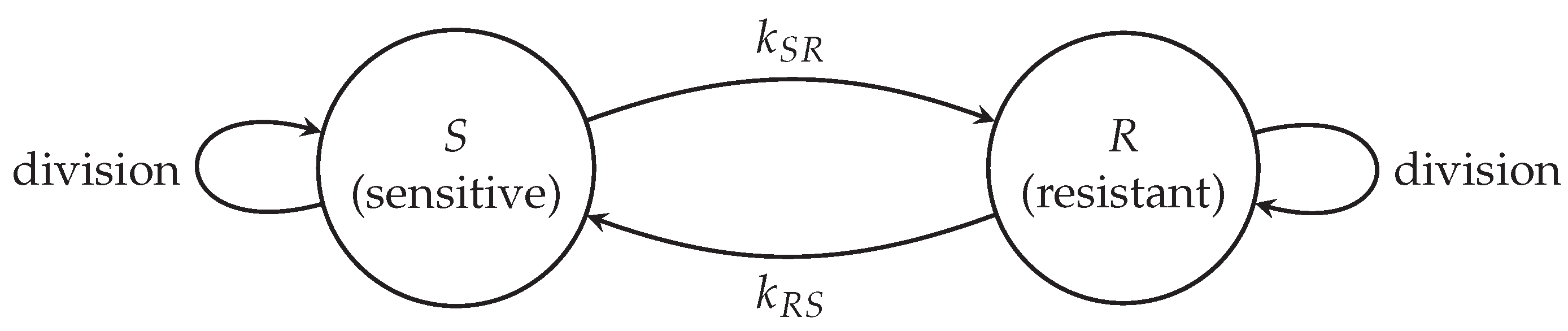
Figure 2.
Local truncation error convergence for c, d, and o using ADI across , validating second-order spatial accuracy.
Figure 2.
Local truncation error convergence for c, d, and o using ADI across , validating second-order spatial accuracy.
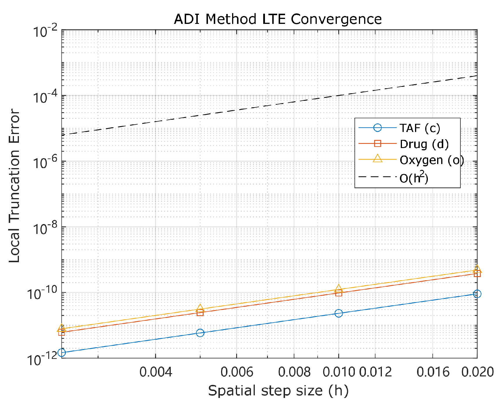
Figure 3.
Stability condition characterization. Admissible region consistent with Theorem 6’s CFL-type bound.
Figure 3.
Stability condition characterization. Admissible region consistent with Theorem 6’s CFL-type bound.
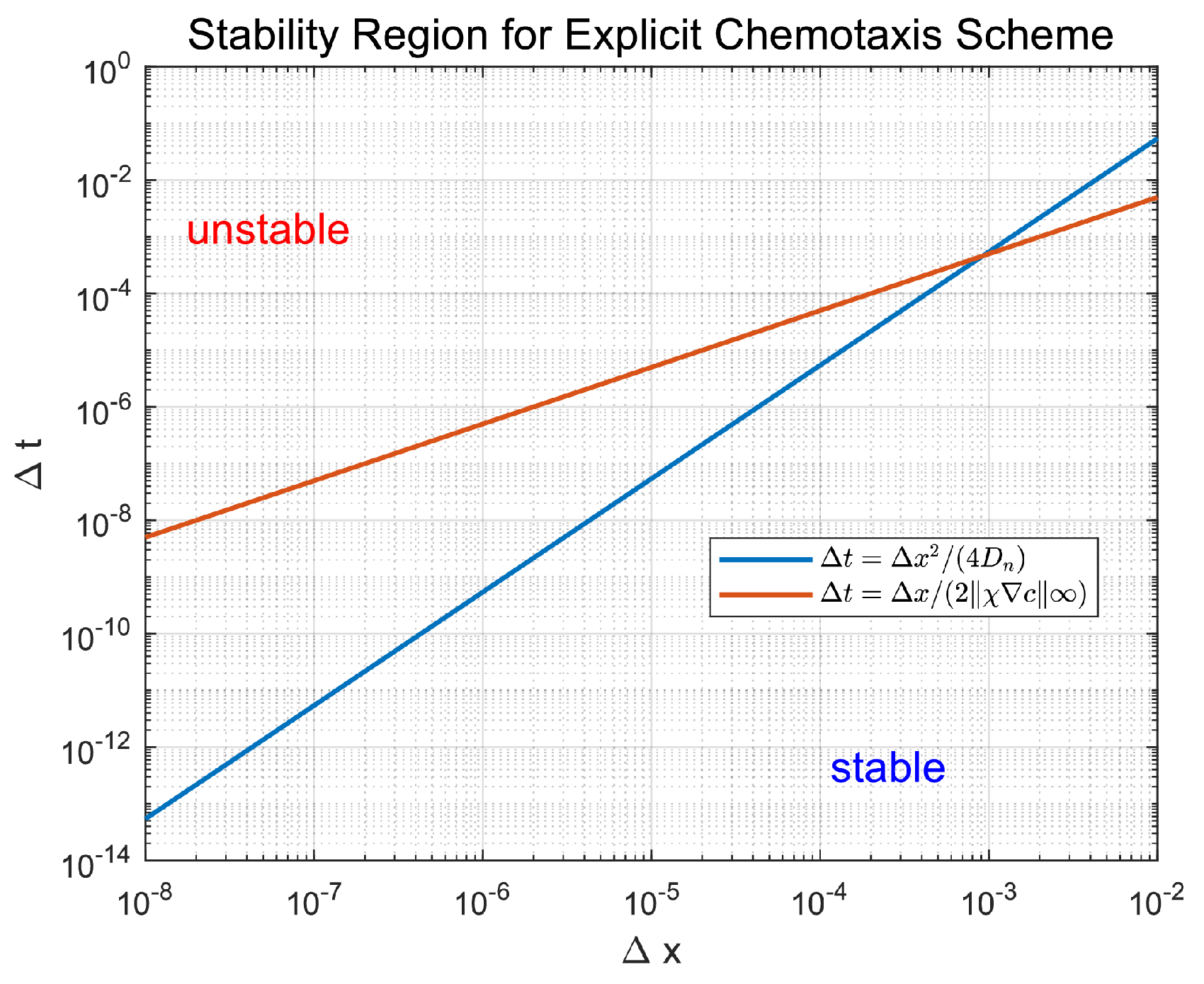
Figure 4.
The maximum norm for the oxygen and TAF fields is shown plotted against t, for grid spacings , , and . Fixed time steps and are used. The near-identical decay slopes beyond verify asymptotic stability and second-order spatial consistency of the PDE solver.
Figure 4.
The maximum norm for the oxygen and TAF fields is shown plotted against t, for grid spacings , , and . Fixed time steps and are used. The near-identical decay slopes beyond verify asymptotic stability and second-order spatial consistency of the PDE solver.
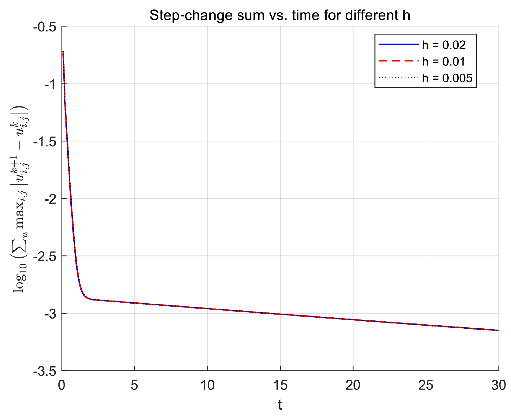

Table 1.
Table 1 provides the complete parameters for the hybrid model. It categorizes parameters into partial differential equation (PDE) systems, agent-based models (ABMs), and numerical parameters. Entries marked "n/a" denote non-applicable or unavailable parameters.
Table 1.
Table 1 provides the complete parameters for the hybrid model. It categorizes parameters into partial differential equation (PDE) systems, agent-based models (ABMs), and numerical parameters. Entries marked "n/a" denote non-applicable or unavailable parameters.
| Parameter | Description | Dimensional Value | Non-Dimensional Value | Source |
|---|---|---|---|---|
| PDE Parameters | ||||
| Endothelial cell diffusion coefficient | [13] | |||
| Tumor angiogenic factor (TAF) diffusion coefficient | 0.12 | [24,25] | ||
| Drug diffusion coefficient | Scaled | 0.5 | Scaled | |
| Oxygen diffusion coefficient | 0.64 | [26] | ||
| Max chemotactic sensitivity | 0.38 | [13] | ||
| Chemotaxis saturation parameter | Scaled | 0.6 | [13] | |
| TAF decay rate | 0.002 | [27] | ||
| Drug decay rate | Scaled | 0.01 | [17] | |
| Oxygen decay rate | 0.025 | [28] | ||
| TAF production rate | [29] | |||
| TAF uptake rate | n/a, nondimensionalized | 0.1 | [13] | |
| Drug uptake rate by tumor cells | Scaled | 0.5 | [17] | |
| Oxygen uptake rate by tumor cells | 34.39 | [17] | ||
| Drug supply rate from vessels | Scaled | 2 | [17] | |
| Oxygen supply rate from vessels | Calibrated | 3.5 | Calibrated | |
| U | Spatial domain | n/a | n/a | Bounded subset of with boundary |
| ABM Parameters | ||||
| Cell radius for tumor and endothelial cells | 0.005 | [30] | ||
| Characteristic functions for tumor and vessel agents | n/a | [22] | ||
| , , , , | Tumor, normoxic, hypoxic, tip and vessel cell sets at time t | n/a | n/a | [22] |
| , , | Positions of , , at time t | n/a | n/a | [22] |
| , , , , , | Local oxygen, drug level, damage, death threshold, age, and cell cycle for tumor cell | n/a | n/a | [22] |
| Tip cell b’s age | n/a | n/a | [22] | |
| Phenotype marks (sensitive S or resistant R) | n/a | n/a | Gillespie algorithm | |
| Tumor movement rate | Modeling choice | 0.01 | Modeling choice | |
| Maximum oxygen level | 1 | [29] | ||
| Hypoxia threshold for tumor cells | Threshold setting | 0.25 | [29] | |
| Apoptosis threshold for tumor cells | Threshold setting | 0.05 | [29] | |
| Sensitive-to-resistant mutation rate | n/a | Gillespie algorithm | ||
| Resistant-to-sensitive mutation rate | n/a | Gillespie algorithm | ||
| Total propensity | n/a | n/a | Gillespie algorithm | |
| DNA Damage clearance rate | Scaled | 0.2 | [17] | |
| Death threshold ratio | 100–1000 | 100–1000 | [31] | |
| Cell cycle duration | 0.56-0.69 | [32,33,34,35,36,37] | ||
| Normoxic proliferation rate | Derived from | 1.0082-1.2323 | Derived | |
| Crowding threshold for proliferation | Modeling choice | 10 | [38] | |
| Tip cell branching age threshold | Scaled | 0.5 | [13] | |
| Branching intensity coefficient | Modeling choice | 1 | [38] | |
| Endothelial cell remaining stationary or moving left, right, down, or up probabilities | n/a | n/a | [22] | |
| Numerical Parameters | ||||
| Spatial discretization step | m | 0.01 | Courant–Friedrichs–Lewy (CFL) condition | |
| PDE Temporal discretization step | s | 0.005 | CFL condition | |
| ABM update time step | s | 0.1 | Modeling choice | |
| Domain side length | m | 1 | [22] | |
| Grid size | n/a | 99 | Modeling choice | |
| Domain smoothing radius | n/a | Algorithm 1 | ||
| Domain threshold for | n/a | Small | Algorithm 1 | |
Table 2.
Discretization parameters and numerical schemes for the hybrid PDE-ABM system. ADI handles reaction-diffusion fields while endothelial chemotaxis updates explicitly under the CFL constraint.
Table 2.
Discretization parameters and numerical schemes for the hybrid PDE-ABM system. ADI handles reaction-diffusion fields while endothelial chemotaxis updates explicitly under the CFL constraint.
| Parameter | Value | Description |
|---|---|---|
| Domain size | Physical size | |
| 1 | Nondimensional domain length | |
| Grid spacing | ||
| PDE time step | ||
| ABM update interval | ||
| Grid points | 100 | Grid node count |
| PDE scheme | ADI (semi-implicit) | Diffusion implicit, reaction explicit |
| PDE scheme n | Euler (explicit) | Subject to CFL condition |
| Boundary conditions | Neumann (no-flux) | All boundaries |
| Stability | Verified | CFL satisfied |
Table 3.
Computed local truncation error orders for across spatial resolutions.
| h | ||||
|---|---|---|---|---|
| n/a | n/a | n/a |
Table 4.
Maximum temporal step changes and logarithmic decay rates from Figure 4 for spatial resolutions . All simulations use fixed and (see Table 2). Least-squares slopes of are computed over . The consistent magnitudes and slopes confirm spatial consistency and numerical stability.
| Grid spacing h | Step size | Step size | Max norm at | Slope of |
|---|---|---|---|---|
Disclaimer/Publisher’s Note: The statements, opinions and data contained in all publications are solely those of the individual author(s) and contributor(s) and not of MDPI and/or the editor(s). MDPI and/or the editor(s) disclaim responsibility for any injury to people or property resulting from any ideas, methods, instructions or products referred to in the content. |
© 2025 by the authors. Licensee MDPI, Basel, Switzerland. This article is an open access article distributed under the terms and conditions of the Creative Commons Attribution (CC BY) license (http://creativecommons.org/licenses/by/4.0/).
Copyright: This open access article is published under a Creative Commons CC BY 4.0 license, which permit the free download, distribution, and reuse, provided that the author and preprint are cited in any reuse.


