A PDE Model of Glioblastoma Progression: the Role of Cell Crowding and Resource Competition in Proliferation and Diffusion

1. Introduction

Glioblastoma, the most aggressive form of primary brain tumor, remains one of the most challenging malignancies to address in both clinical practice and biomedical research [1]. This cancer is distinguished by its rapid proliferation, diffuse infiltration into healthy brain tissue, and marked resistance to conventional therapeutic modalities [2,3,4]. Despite significant efforts to improve treatment strategies, including maximal surgical resection, temozolomide-based chemotherapy, and radiotherapy, the median survival for glioblastoma patients remains dismally low, rarely exceeding 15 months [5]. Factors contributing to this grim prognosis include the tumor’s remarkable heterogeneity, its ability to evade immune surveillance, and its reliance on complex interactions within the tumor microenvironment. Collectively, these challenges highlight an urgent need for innovative approaches that go beyond traditional therapeutic paradigms [6,7,8,9].

A critical aspect of glioblastoma’s complexity lies in its invasive nature. Unlike many solid tumors, glioblastoma cells infiltrate diffusely into surrounding brain tissue, often migrating far beyond the visible tumor margins observed in imaging [10,11]. This behavior severely limits the efficacy of surgical resection and contributes to inevitable tumor recurrence. Additionally, glioblastoma exhibits significant intratumoral heterogeneity at the genetic, epigenetic, and phenotypic levels, leading to varied responses to therapy and the emergence of treatment-resistant subpopulations. Understanding and addressing this intricate biological behavior necessitate advanced tools capable of capturing its underlying dynamics [12,13].

In this regard, mathematical modeling and computational simulation have emerged as powerful frameworks for studying glioblastoma. By leveraging mathematical abstractions, these approaches enable researchers to synthesize biological data into coherent models that describe tumor behavior at multiple scales, from molecular signaling pathways to macroscopic tumor growth. These models serve several critical purposes: they provide insights into the mechanisms driving tumor progression, offer predictive capabilities for treatment outcomes, and suggest novel therapeutic targets. Importantly, mathematical models are not confined to theoretical exploration, but they can also be directly integrated with experimental data to refine hypotheses, improve model accuracy, and support clinical decision-making [14,15,16,17,18,19].

Numerous researchers have made significant contributions to the mathematical modeling of glioblastoma, developing a diverse array of frameworks to study its growth, invasion, and therapeutic responses. For example, Stein et al. [20] proposed a model that quantitatively describes the evolution of both the invasive and central radii of glioblastoma over time, linking tumor morphology to its underlying dynamics. This work laid a foundation for understanding how macroscopic tumor growth reflects biological processes at smaller scales. Conte and Surulescu [21] advanced this field further by presenting a multiscale model that incorporates tissue anisotropy, capturing the heterogeneous nature of the brain environment and its impact on glioblastoma invasion. Such models illustrate the importance of integrating spatial and structural complexities into computational frameworks.

Reviews of glioblastoma modeling efforts have further enriched the field by synthesizing existing approaches and identifying gaps in knowledge. For instance, Falco et al. [22] provided a comprehensive analysis of various mathematical models, categorizing them based on their biological assumptions and computational methodologies. Their work highlighted the progress achieved in areas such as reaction-diffusion models, agent-based simulations, and multiscale modeling, while also emphasizing the need for more refined models that account for tumor-microenvironment interactions and adaptive resistance mechanisms. Similarly, studies by Hatzikirou et al. [19], Engwer et al. [23], Kumar et al. [24], Jørgensen et al. [25] have introduced novel frameworks that address specific aspects of glioblastoma dynamics, including the stochastic nature of cell migration [26], angiogenesis, and the impact of therapeutic interventions. Regarding the modeling of the angiogenic mechanisms supporting tumor invasion, we mention the fine model developed by Gandolfi et al. [27], which accounts for vessel cooption and chemotaxis stimulated by pro-angiogenic factors.

Beyond theoretical advancements, mathematical models have practical implications for glioblastoma research and treatment. By simulating various therapeutic scenarios, these models can identify optimal dosing regimens, predict the likelihood of recurrence, and evaluate the efficacy of combination therapies. Furthermore, they provide a platform for testing hypotheses about glioblastoma biology, such as the role of hypoxia in driving tumor invasion or the impact of phenotypic plasticity on resistance. As experimental techniques continue to generate high-resolution data, from single-cell transcriptomics to live imaging of tumor growth, mathematical models are poised to integrate these datasets into predictive tools for precision oncology. For these reasons, glioblastoma represents a critical frontier for mathematical modeling and computational simulation. By synthesizing biological knowledge with mathematical rigor, these approaches offer a unique perspective on the complex interplay of factors driving glioblastoma progression and resistance. The continued refinement of these models, coupled with advances in experimental and clinical research, holds great promise for transforming our understanding of this devastating disease and improving outcomes for patients.

In this work, we address the mathematical modeling and simulation of glioblastoma spread. Building upon our previous studies [28,29], we aim to advance the current understanding of glioblastoma dynamics through a more robust theoretical framework. The work by Pompa et al. [28] introduced an Agent-Based Model (ABM) to simulate glioblastoma infiltration into healthy brain tissue, accounting for cell motility and proliferation rates influenced by internal energy levels. In the subsequent study by Borri et al. [29], the glioblastoma infiltration was described by means of a continuum-scale PDE-based approach, comparing different probability distributions in reproducing experimental data on the spatial spread of grioblastoma cells. In the present study, we deepen the PDE-based data analysis introduced in Borri et al. [29], improving the model formulation and focusing on different aspects of cell physiology. Specifically, we propose an improved reaction-diffusion PDE formulation that better captures the essential features of glioblastoma growth and diffusion, along with a model-based characterization of the tumor core and invasion front radii. Moreover, we investigate the effect of cell crowding and resource competition in the limitation of cell growth and diffusion, showing their relevant role in the tumour spread.

Organization. The paper is structured as follows. Section 2 introduces the mathematical tools and concepts used throughout the work. Section 3 presents the glioblastoma infiltration modeling framework and the experimental data employed. Section 4 outlines the optimization problem for parameter identification. Simulation results and their discussion are provided in Section 5. Finally, Section 6 offers concluding remarks.

Notation. In the paper we adopt the following notation. We denote by ${\mathbb{R}}_{+}$ the set of nonnegative real numbers. Given a vector field $f:{\mathbb{R}}^n\to {\mathbb{R}}^n$ the divergence operator in Cartesian coordinates is defined by $div\left(F\right)={\sum }_{i=1}^n{\displaystyle \frac{\partial F_i}{\partial x_i}}$, while the Laplace operator of a function $f:{\mathbb{R}}^n\to \mathbb{R}$ is defined by ${\nabla }^{2}f={\sum }_{i=1}^n{\displaystyle \frac{{\partial }^{2}f}{\partial x_i^2}}$. We define by $\delta \left(x^0\right)$ the Dirac delta function centered at $x^0\in {\mathbb{R}}^n$. If x is a vector in ${\mathbb{R}}^n$, then its Euclidean norm is given by $\parallel x\parallel$, namely $x^{\top }x={\parallel x\parallel }^2$. We denote by I the identity matrix of appropriate dimension.

2. Mathematical Framework

We illustrate in this section the mathematical framework for describing higher-dimensional/complexity models that exhibit certain properties of symmetry and/or isotropy, similar to those explored later in this study.

2.1. Stochastic differential equations and the Fokker-Planck equation

A Stochastic Differential Equation (SDE) of an n-dimensional Itô process $X\left(t\right)=(X_1\left(t\right),\dots ,X_n\left(t\right))$ is given by

$$dX\left(t\right)=-b\left(X\left(t\right)\right)dt+\sigma dW\left(t\right),X\left(0\right)\sim p_0,$$

(1)

where $W\left(t\right)$ is an n-dimensional Wiener process, $b\left(x\right):{\mathbb{R}}^n\to {\mathbb{R}}^n$ is the drift term, $\sigma :=\sqrt{2D}$ with $D>0$ the so-called diffusion coefficient, $p_0\left(x\right)$ a multidimensional initial ($t=0$) probability density function with $x={[x_1\dots x_n]}^{\top }\in {\mathbb{R}}^n$ the vector of Cartesian coordinates in the n-dimensional space ($n\in \{1,2,3\}$). At each subsequent time $t>0$, the particles are observed to be distributed non-uniformly throughout space, according to a probability density function $p:{\mathbb{R}}_{+}\times {\mathbb{R}}^n\to {\mathbb{R}}_{+}$. It is well known that this underlying probability density function p satisfies the Fokker-Planck equation

$${\displaystyle \frac{\partial p(t,x)}{\partial t}}=div(\left(b\left(x\right)p(t,x)\right)+D{\nabla }^{2}p(t,x),p(0,x)=p_0\left(x\right).$$

(2)

Since the solution $p(t,x)$ to (2) is a probability density on ${\mathbb{R}}^n$ for almost every fixed time t, then $p(t,x)\ge 0$ for almost every $(t,x)\in {\mathbb{R}}_{+}\times {\mathbb{R}}^n$ and ${\int }_{{\mathbb{R}}^n}p(t,x)d{x}_1\dots d{x}_n=1$ for every $t\ge 0$.

In some particular cases, it is possible to give the explicit expression of the stationary probability density function satisfying the Fokker-Plank equation (2). For instance, if the drift coefficient is given by a vector field $b\left(x\right)=\nabla \mathsf{\Psi }\left(x\right)$[30], where $\mathsf{\Psi }:{\mathbb{R}}^n\to {\mathbb{R}}_{+}$ is a smooth function that meets suitable conditions [31], there exists a unique stationary solution $p_s\left(x\right)$ to the Fokker–Planck equation, which is given by the Gibbs density function

$$p_s\left(x\right)=Z^{-1}exp(-D^{-1}\mathsf{\Psi }\left(x\right)),$$

(3)

where the coefficient Z is given by the expression

$$Z:={\int }_{{\mathbb{R}}^n}exp(-D^{-1}\mathsf{\Psi }\left(x\right))dx<+\infty .$$

(4)

Furthermore, if the drift term is zero, namely $b\left(x\right)=0$, and the diffusion is still constant as in (2), the process $\left\{X\right(t\left)\right\}$ in (1) is given by

$$dX\left(t\right)=\sigma dW\left(t\right),X^0\sim p_0,$$

(5)

and it is a shifted n-dimensional Wiener process if $p_0\left(x\right)=\delta \left(x^0\right)$, with $x^0\in {\mathbb{R}}^n$. As a consequence, the condition (4) for the existence and uniqueness of the stationary solution fails, and the solution to the Fokker-Planck equation (2), which reduces to

$${\displaystyle \frac{\partial p(t,x)}{\partial t}}=D{\nabla }^{2}p(t,x),p(0,x)=\delta \left(x^0\right),$$

(6)

is the Gaussian density

$$p(t,x)={\displaystyle \frac{1}{{\left(2\pi {\sigma }^{2}t\right)}^{n/2}}}{e}^{-{\displaystyle \frac{1}{2}}{\displaystyle \frac{\parallel x-x^0{\parallel }^2}{{\sigma }^{2}t}}},$$

(7)

describing a continuous-time random walk with mean $x^0$ and covariance ${\sigma }^{2}tI$, linearly increasing with time. It is clear that, since the independent variable x is the vector of the Cartesian coordinates, the latter model implicitly assumes spherical symmetry, as the density centered at $x^0$ exhibits such a kind of symmetry.

The stochastic model reported in this section provides the basic mathematical framework describing the mechanism underlying the ensemble diffusion process characterizing a population with random mobility of the single individuals, which we will extend to more refined models in the remainder of the paper.

2.2. Fisher equation

In this section we present another PDE model which is typically used to describe the spread of a cell population: the Fisher equation [32,33]. This model is actually an extension of the one given above in Eq. (2) since, in addition to the diffusion process, it accounts for the net balance between mass production and elimination. In an n-dimensional space it is given by

$${\displaystyle \frac{\partial u(t,x)}{\partial t}}=div(\left(v\left(x\right)u(t,x)\right)+D{\nabla }^{2}u(t,x)+gu(t,x)\left(1-{\displaystyle \frac{u(t,x)}{u_{m}ax}}\right),u(0,x)=u_0\left(x\right),$$

(8)

where the solution $u:{\mathbb{R}}_{+}\times {\mathbb{R}}^n\to \mathbb{R}$ is the scalar field representing, for example, population density or concentration at position $x\in {\mathbb{R}}^n$ and time $t>0$. Similarly as before, the vector $v\left(x\right):{\mathbb{R}}^n\to {\mathbb{R}}^n$ is a drift term, the constant $D>0$ is the diffusion coefficient, while $g>0$ is the proliferation rate constant, and $u_{m}ax$ is the local carrying capacity of the cells representing the maximal cell density that can be reached by the solution u (at any point), related to environmental and nutrient conditions, as well as to cell competition. Unlike the Fokker-Planck equation, which is a partial differential equation (PDE) describing the evolution of a probability density function typically derived from an underlying Itô process accounting only for motility aspects, the Fisher equation is a reaction-diffusion equation that models both spread and proliferation of a biological population. This is essentially obtained by considering the additive logistic-type growth term to the previous Fokker-Plank equation (suitably scaling the probability density to the cell/mass density).

3. Glioblastoma Infiltration Modeling

We now leverage the mathematical framework developed in the preceding section to formulate suitable macroscopic/mesoscopic models that capture the experimental time-behaviour of a Glioblastoma tumour mass. In particular, from the paper by Stein et al. [20] we retrieved experimental data on cell density and on two radii characterizing the time-volution of the tumour mass. So, we propose three different models with the aim of explicitly reproducing these kinds of variables. Moreover, the three proposed models intentionally exhibit increasing complexity (from the one given in SubSection 3.2.1 to the last one in SubSection 3.2.3) exploited to highlight the impact on the tumour evolution of specific physiological processes, as cell proliferation, and some mechanisms limiting both diffusion and proliferation (like cell crowding and resource competition). All the proposed models incorporate the following key features:

• polar coordinate formulation: because of the assumption of symmetry and isotropy of cell movements (already assumed in Pompa et al. [28]) within the tumour mass we can reduce the spatial dependency to only the radial coordinate;
• model outputs reproducing the available data on two different cell lines: U87WT (already considered in [28]) and U87$\Delta$EGFR, which is a common mutation (data reported in Stein et al. [20], see the next section); the proposed models are specified to the different cell lines by means of a suitable parameter estimation.

3.1. Data Collection

In this study, we utilize the experimental data provided by Stein et al. [20], related to the two glioblastoma cell lines U87WT and U87$\Delta$EGFR (a common mutation variant). In that work, the data were extracted through image processing of digital photomicrographs taken at the midplane of spheroids. We consider the following data:

• the invasive radius, ${\overline{R}}_{inv}$, of a tumor that represents the maximum distance that a single tumor cell or a small group of tumor cells can migrate from the primary tumor mass into the surrounding tissue. It is a key parameter in cancer invasion studies, reflecting the ability of malignant cells to infiltrate the extracellular matrix (ECM), evade immune responses, and establish metastases. In [20] it is defined as the farthest distance from the center at which the azimuthally averaged gradient magnitude reaches half of its maximum value;
• the core radius, ${\overline{R}}_{core}$, refers to the central region of the tumor where cell proliferation is significantly reduced or halted due to limited nutrient and oxygen availability. This region is often characterized by hypoxia, necrosis, or quiescence, depending on the severity of the nutrient and waste diffusion limitations. In Stein et al. [20] the region is defined as the collection of pixels exhibiting an intensity level of $0.12$ on a grayscale image—where 0 corresponds to the darkest pixel and 1 to the brightest—centered around the tumor spheroid;
• the radial cell density at day 3 (expressed in [${\mathrm{cells/cm}}^3$]), function of the radius $r>0$, that is denoted by $\overline{u}(\overline{t},r)$ with $\overline{t}=3$; it is extracted based on the concentration of darker pixels observed in the digital photomicrograph data.

Specifically, we aim to replicate the experimental trends shown in Figure 2 (panels A–C) of Stein et al. [20], which include: the temporal evolution of the invasive radius (panel A) and the core radius (panel B) of the tumor from day 0 to day 7, and the radial cell density profile at day 3 (panel C).

3.2. Radial Distribution Models of Invasive Cells

In this section we propose three different models for the radial position of the invasive tumour cells on a three-dimensional space ($n=3$), under the hypothesis of spherical symmetry. In particular, we describe by means of PDEs the spatial distribution of the cell density $u(t,r)$ (measurement unit [${\mathrm{cells/cm}}^3$]), with $u:{\mathbb{R}}_{+}\times \mathbb{R}\to \mathbb{R}$, where the spatial dependence of u is reduced to the single radial coordinate r, because of the spherical symmetry hypothesis. Under this simplifying assumption, the Laplace operator in the 3D space becomes

$${\nabla }^{2}u(t,r)={\displaystyle \frac{2}{r}}{\displaystyle \frac{\partial u(t,r)}{\partial r}}+{\displaystyle \frac{{\partial }^{2}u(t,r)}{\partial r^2}},$$

(9)

because the derivatives with respect to the angle coordinates are trivially zero ($\partial \theta /\partial r=\partial \varphi /\partial r=0$). All the proposed models have zero drift terms.

The models are then complemented by initial and boundary conditions as follows. Concerning the initial condition, we set $u(0,r)=u_0\left(r\right)$ with

$$u_0\left(r\right)=\left\{\begin{array}{cc}\overline{u},\hfill & \mathrm{for}r\le R_0,\hfill \\ 0,\hfill & \mathrm{for}r>R_0,\hfill \end{array}\right.$$

(10)

where $R_0$ is the initial radius of the implanted tumor mass and $\overline{u}>0$ the related (constant) cell density. As far as the boundary conditions are concerned, the cell density is subject to the common zero flux conditions at $r=0$ because of the domain symmetry, i.e. ${\displaystyle \frac{\partial u(t,r)}{\partial r}}{|}_{r=0}=0$. Assuming also that the cell density is zero far from the tumour mass, we impose the second boundary condition $u(t,\infty )=0$.

According to the definition given in [20] based on grayscale images, we mathematically define the core radius $R_{c}ore\left(t\right)$ and the invasive radius$R_{i}nv\left(t\right)$ at time $t>0$, for all the proposed models, as

$$R_{core}\left(t\right):=min\left\{\overline{r}:\left(1-{\displaystyle \frac{u(t,\overline{r})}{u(t,0)}}\right)\ge 0.12\right\},R_{inv}\left(t\right):=min\left\{\overline{r}:\left(1-{\displaystyle \frac{u(t,\overline{r})}{u(t,0)}}\right)\ge 0.98\right\}.$$

(11)

The intuition behind the formulae (11) is that, at each time t, core and invasive radii are defined as the radial coordinates such that the cell density at these points decreases to $88\%$ and $2\%$, respectively, of the cell density $u(t,0)$ in the tumour center. These definitions are different and simpler with respect to the one proposed in [29], given in terms of percentile of the tumor cell cumulative distribution function. In particular, the $12\%$ threshold set for the core radius definition matches the value $0.12$ of the normalized light intensity chosen in [20] to identify the core from the grey-scale images obtained from digital photomicrographs of the corresponding spheroid (see also SubSection 3.1), while the $98\%$ value for the invasive radius has been calibrated in this work; however, note that the chosen threshold for the invasive radius is in agreement with the ones chosen in [20], ranging in the interval $(0.98,1)$. Note that at the initial time (tumour implantation) $R_{c}ore\left(0\right)=R_{i}nv\left(0\right)=R_0$.

As mentioned in Section 3.1, the core and the invasive radii are increasing in the observation period, so a steady-state model of cell distribution would not be realistic. Therefore, we focus on three different time-varying models for the cell density $u(t,r)$: i) a Pure Diffusive (PD) model (i.e., the Fokker-Planck equation), ii) a model combining Diffusion and Growth (DG), with a standard logistic-type limitation factor of cell growth due to nutrient availability (i.e., the Fisher equation), and iii) a more refined model accounting for limitations of both diffusion and growth, which introduces more general modulation factors representing the impact of cell crowding and resource competition (Modulated Growth and Diffusion model, MDG).

3.2.1. Pure Diffusion Model (PD)

The simplest non-stationary model we can define for the position of tumor cells, defined by a process $\left\{X\right(t\left)\right\}$, is the pure diffusive case exploited in (5) (no drift or cell proliferation), where we assume that the origin of the Cartesian frame is set in the center of the tumor spheroid. Thus, under the symmetry hypothesis of the 3D domain, the associated PDE in radial coordinates describing the cell density distribution is given by

$${\displaystyle \frac{\partial u}{\partial t}}=D\left({\displaystyle \frac{2}{r}}{\displaystyle \frac{\partial u(t,r)}{\partial r}}+{\displaystyle \frac{{\partial }^{2}u(t,r)}{\partial r^2}}\right),$$

(12)

with initial and boundary condition reported in Section 3.2. For this model, the parameters to be identified are ${\mathsf{\Theta }}^{PD}:=\{D,\overline{u}\}$, where $\overline{u}$ is defined in (10), that are computed through an optimization problem (see Section 4). In the following, we denote by $u^{PD}(t,r)$ the solution to the pure diffusion equation.

Notice that, in view of the pure diffusion process considered, the total number of cells M (i.e. the tumour mass) is constant over time (since no cell birth/death processes are taken into account by the model) and it is given by the relation $M:={\int }_{{\mathbb{R}}^n}u(t,r)dV={\int }_{{\mathbb{R}}^n}u(0,r)dV$, where $dV$ is the infinitesimal volume element in spherical coordinates and $n=3$ (i.e., $dV=r^{2}sin\theta d\theta d\varphi dr$ where $\theta$, $\varphi$ are the angle coordinates). According to the previous definition, we have $M=4\pi {\int }_0^{R_0}\overline{u}{r}^{2}dr=\left({\displaystyle \frac{4}{3}}\pi R_0^3\right)\overline{u}$. It is also interesting to notice that, as the corresponding probability density function of the tumour population $p(t,r)$ is characterized by the basic property ${\int }_{{\mathbb{R}}^n}p(t,r)dV=1$, the total number of cells M represents a constant coefficient for rescaling the cell density to the probability density function (and vice-versa), i.e., $p(t,r)=u(t,r)/M$. Moreover, if the initial condition of Eq. (12) is set as in Eq. (6) (describing the probability density p of the population), i.e. $u(0,r)=M\delta \left(0\right)$ (the whole tumour population is trivially concentrated in $r=0$ at $t=0$), it is interesting to look at the related stochastic process given by $\rho \left(t\right):=\parallel X\left(t\right)\parallel$, which has a noncentral chi distribution given by

$$\rho \left(t\right)=\sqrt{\sum _{i=1}^n{X}_i^2}\sim p_{PD}(t,r):=e^{-{\displaystyle \frac{r^2/\left({\sigma }^{2}t\right)+{\lambda }^2}{2}}}{\displaystyle \frac{r^{n/2}\lambda }{{\left(\sigma \sqrt{t}\right)}^{(n+2)/2}{\lambda }^{n/2}}}{J}_{n/2-1}\left({\displaystyle \frac{\lambda r}{\sigma \sqrt{t}}}\right),t\ge 0,r>0,$$

(13)

where $\lambda ={\displaystyle \frac{1}{\sigma \sqrt{t}}}\sqrt{{\sum }_{i=1}^n{x_i^0}^2}$, with $x^0=\left(x_1^0,\dots ,x_n^0\right)$ the initial condition, and $J_{\alpha }(·)$ the Bessel functions of the first kind ([34]). Although the model (12) provides a simple basis for comparison and allows for approximate computations over a short time horizon, its underlying behavior is not realistic given the invasive and reproductive nature of tumor cells. In the following subsections, the model will be properly extended to account for the growing cancer cell population.

3.2.2. Diffusion and Growth Model (DG)

A more detailed model consists in considering the reaction-diffusion equation by Fisher, given above in Section 2.2. According to the assumptions given in Section 3.2 and neglecting additional cell movement sources out of the diffusion (i.e., $v=0$), the Fisher equation in radial coordinates becomes

$$\begin{array}{cc}\hfill {\displaystyle \frac{\partial u(t,r)}{\partial t}}& =D\left({\displaystyle \frac{2}{r}}{\displaystyle \frac{\partial u(t,r)}{\partial r}}+{\displaystyle \frac{{\partial }^{2}u(t,r)}{\partial r^2}}\right)+gu(t,r)\left(1-{\displaystyle \frac{u(t,r)}{u_{max}}}\right),\hfill \end{array}$$

(14)

with initial and boundary condition reported in Section 3.2. In the following, we denote by $u^{DG}(t,r)$ the solution to the Fisher model equation (14), which depends on the parameters ${\mathsf{\Theta }}^{DG}:=\{D,\overline{u},g,u_{max}\}$ that are computed through an optimization problem (see Section 4). Note that model (14) extends the simple pure-diffusion one (12) because of the presence of the logistic term reproducing the net cell proliferation coming from a birth/death balance.

3.2.3. Modulated Diffusion and Growth Model (MDG)

The final model we propose is an enhanced version of the previous Fisher model, extending the modulation of the proliferation rate constant g (already present in Eq. (14)) and introducing a further modulation of the diffusion constant D. As explained in the seminal paper [27], in crowded environments there is an increasing impairment of cell movement and an increasing inhibition of cell proliferation as cell density increases. Such phenomena are likely to follow different laws with respect to cell density. As done in [27,35], in the last proposed model we take both these phenomena into account by multiplying proliferation rate constant and diffusion coefficient by means of the following limiting factor

$${\left(1-{\displaystyle \frac{u}{u_{max}}}\right)}^{\alpha },\alpha >0.$$

However, we assume that the extent of the limitation can be different for the diffusion and the proliferation, and then we assume that the exponent $\alpha$ can be different (in principle) for the two mechanisms. According to this modeling setting, we give the following modified Fisher equation

$$\begin{array}{cc}\hfill {\displaystyle \frac{\partial u(t,r)}{\partial t}}& =D{\left(1-{\displaystyle \frac{u(t,r)}{u_{m}ax}}\right)}^{{\alpha }_D}\left({\displaystyle \frac{2}{r}}{\displaystyle \frac{\partial u(t,r)}{\partial r}}+{\displaystyle \frac{{\partial }^{2}u(t,r)}{\partial r^2}}\right)+gu(t,r){\left(1-{\displaystyle \frac{u(t,r)}{u_{m}ax}}\right)}^{{\alpha }_g},\hfill \end{array}$$

(15)

with initial and boundary condition reported in Section 3.2. In the following, we denote by $u^{MDG}(t,r)$ the solution to model equation (15), depending on the parameters ${\mathsf{\Theta }}^{MDG}=\{D,\overline{u},g,u_{max},{\alpha }_g,{\alpha }_D\}$ that are computed through an optimization problem (see Section 4).

Remark 1. 

As a final remark on the proposed modeling framework, we highlight that, as already mentioned above, the pure diffusion model (13) does not incorporate any aspects of cell proliferation, so we expect a worse performance in the fitting of the time-varying quantities, such as the core and invasive radii. We also note that the extended modulation of cell proliferation and diffusion introduced in model (15) (due to cell crowding and competition to resources) gives to this model more degrees of freedom w.r.t. model (14) in reproducing the experimental data.

4. Parameter Identification

In this section, we discuss the optimization problem used to identify the model parameters. We consider the three sets of data:

i) 

$m_u={\left\{\overline{u}(\overline{t},r_k)\right\}}_{k=1}^{N_u}$ representing the radial distribution of cell density on days $t=\overline{t}=3$, measured at different spatial points $r_k$ with a sample size $N_u$;

ii) 

$m_{core}={\left\{{\overline{R}}_{c}ore\left(t_k\right)\right\}}_{k=1}^{N_{core}}$ representing the core radius at different times $t_k$, with a sample size $N_{core}$;

iii) 

$m_{inv}={\left\{{\overline{R}}_{i}nv\left(t_k\right)\right\}}_{k=1}^{N_{inv}}$ representing the invasive radius at different times $t_k$, with a sample size $N_{inv}$.

All data are retrieved from Stein et al. [20]. Denoting by $u^{\Sigma }(t,r)$ the solution of model $\Sigma$, with $\Sigma \in \{PD,DG,MDG\}$, for any time $t>0$ and radius $r>0$, as well as by ${\mathsf{\Theta }}^{\Sigma }$ and by $R_{core}^{\Sigma }$, $R_{inv}^{\Sigma }$ the vector of related parameters and, respectively, the core and invasive radii (computed according to Eqs. (11) and to the solution $u^{\Sigma }(t,r)$), we define the following optimization problem for the estimation of ${\mathsf{\Theta }}^{\Sigma }$:

$$\begin{array}{cc}\hfill \underset{{\mathsf{\Theta }}^{\Sigma }}{min}{\epsilon }_u^{\Sigma }\sum _{k=1}^{N_u}& ∥\overline{u}(\overline{t},r_k)-u^{\Sigma }(\overline{t},r_k)∥+{\epsilon }_{c}or{e}^{\Sigma }\sum _{k=1}^{N_{core}}∥{\overline{R}}_{c}ore\left(t_k\right)-R_{c}or{e}^{\Sigma }\left(t_k\right)∥\hfill \\ \hfill & +{\epsilon }_{inv}^{\Sigma }\sum _{k=1}^{N_{inv}}∥{\overline{R}}_{i}nv\left(t_k\right)-R_{i}n{v}^{\Sigma }\left(t_k\right)∥.\hfill \end{array}$$

(16)

As the available experimental data are characterized by high differences of magnitude orders and cardinality, the factors weighting the square errors in (16) are set equal to the squared inverse of the product between the cardinality and the mean value of each data set, i.e.

$${\epsilon }_u^{\Sigma }={\displaystyle \frac{1}{{\left(N_u\langle m_u\rangle \right)}^2}},{\epsilon }_{c}or{e}^{\Sigma }={\displaystyle \frac{1}{{\left(N_{core}\langle m_{core}\rangle \right)}^2}},{\epsilon }_{i}n{v}^{\Sigma }={\displaystyle \frac{1}{{\left(N_{inv}\langle m_{inv}\rangle \right)}^2}},$$

(17)

where $\langle ·\rangle$ is the arithmetic mean operator.

5. Simulation Results

The three presented PDE models have been numerically solved in the domain $\mathsf{\Omega }=[0,R_{\infty }]$, where $R_{\infty }$ has been chosen far from the center of the tumour mass ($R_{\infty }=1$ cm, one order of magnitude larger than the highest radius at which the cell density is measured) and in the time span $[0,7]$ days, using the MATLAB solver pdepe (MATLAB^® 2024). The initial tumour radius $R_0$ was fixed at $250\mu$m, value common to the two cell lines and directly measured from the images of the tumour spheroids reported in [20].

The three least-square problems described in Section 4 (minimization of the weighted sum of squared differences between observed and predicted variables) have been solved using the MATLAB^® routine fminsearch for both the available sets of data on the U87WT and U87$\Delta$EGFR cell lines.

Table 1 reports the values of the estimated model parameters, solutions of the three optimization problems, while Figure 1 and Figure 2 show the corresponding best fit of the experimental data (cell density function at $t=3$ days, $R_{c}ore\left(t\right)$ and $R_{i}nv\left(t\right)$ for $t=1,\dots ,7$) for both cell lines, obtained for the three models with optimal parameters. We incidentally note that the estimated diffusion coefficients agree with the values reported in the literature, ranging in the interval ($4.17·{10}^{-7},8.33·{10}^{-6}$) ${\mathrm{cm}}^2$/h [36,37]. Also the estimated proliferation rate constants are basically in agreement with literature data (estimated doubling time around 20 h [20]).

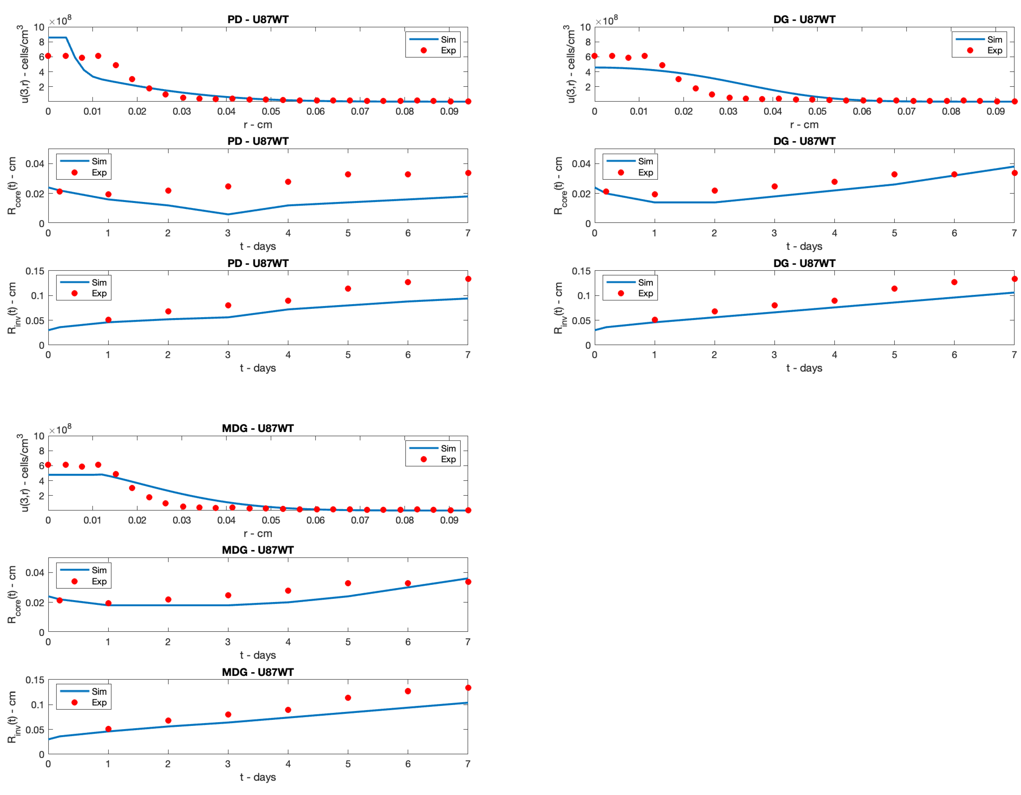
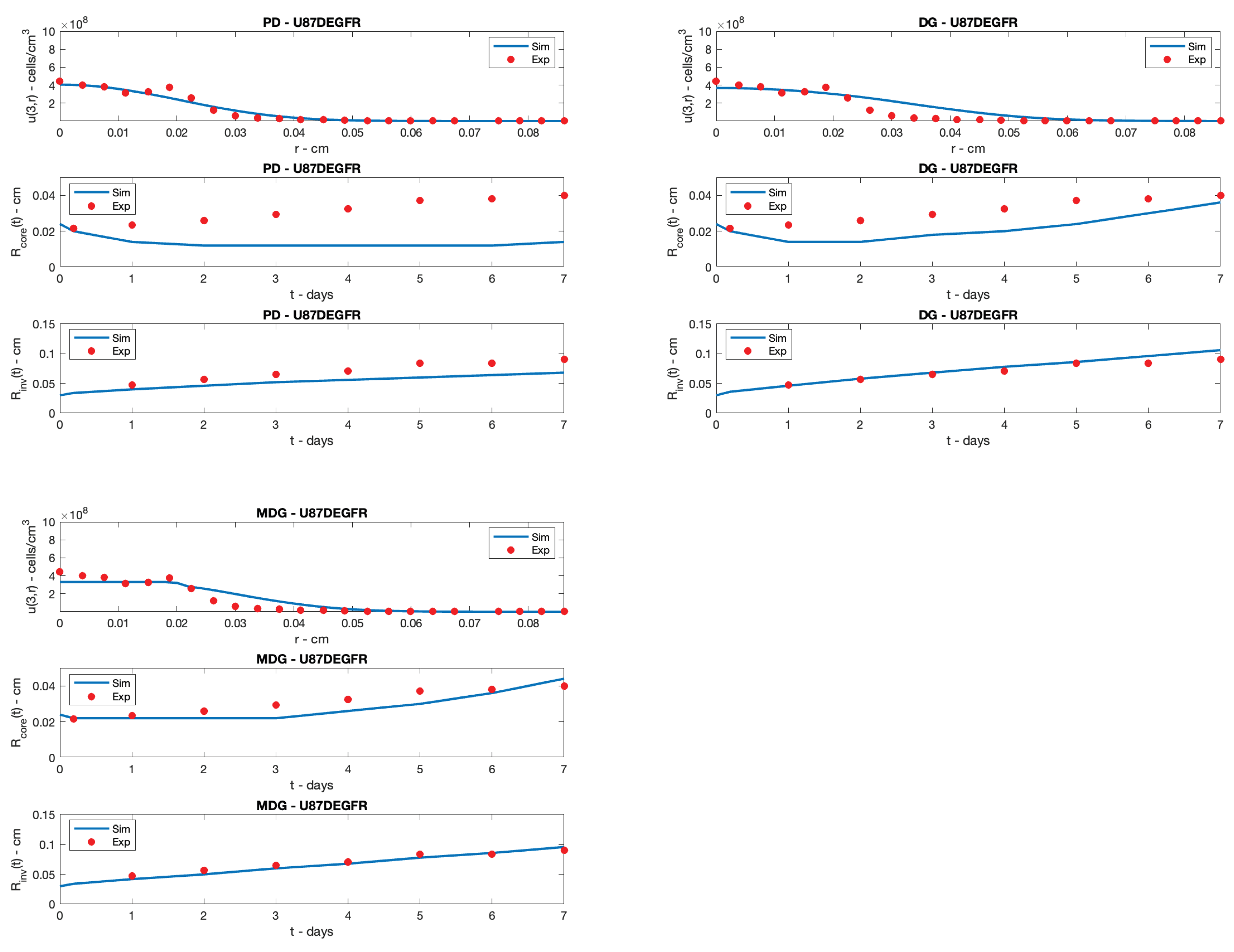
Figure 1. Cell line U87WT: best fit of the experimental cell density at days and of core and invasive radii exploiting the three models; top panel: pure diffusion model (PD); central panel: diffusion-growth model (DG); lower panel: modulated diffusion-growth model (MDG). Red circles: experimental data; blue line: model simulation.

Figure 1. Cell line U87WT: best fit of the experimental cell density at days and of core and invasive radii exploiting the three models; top panel: pure diffusion model (PD); central panel: diffusion-growth model (DG); lower panel: modulated diffusion-growth model (MDG). Red circles: experimental data; blue line: model simulation.

Figure 2. Cell line U87DEGFR: best fit of the experimental cell density at days and of core and invasive radii exploiting the three models; top panel: pure diffusion model (PD); central panel: diffusion-growth model (DG); lower panel: modulated diffusion-growth model (MDG). Red circles: experimental data; blue line: model simulation.

Figure 2. Cell line U87DEGFR: best fit of the experimental cell density at days and of core and invasive radii exploiting the three models; top panel: pure diffusion model (PD); central panel: diffusion-growth model (DG); lower panel: modulated diffusion-growth model (MDG). Red circles: experimental data; blue line: model simulation.

Looking at the fitting results of Figure 1 and Figure 2, as expected the PD model, although coarsely reproducing the cell density profile, cannot follow the time behavior of the data ${\overline{R}}_{core}$ and ${\overline{R}}_{inv}$. In contrast, the other two models show better performances. In particular, it is readily appreciable that the MDG model fits all the data (cell densities and radii of both lines) better than the simpler DG model. So, accounting for the modulation of cell proliferation and diffusion improves the experimental data reproduction.

6. Conclusions

Glioblastoma remains a significant challenge in both clinical practice and research due to its aggressive nature and resistance to current treatments. Mathematical modeling provides a valuable tool to understand the complex dynamics of this disease and to support the development of new therapeutic strategies. In this study, we introduce an improved mathematical model for glioblastoma infiltration. Using a partial differential equation (PDE) framework, we describe the time and space evolution of cancer cell density, capturing both the proliferative and diffusion aspects of the tumor mass, particularly focusing on their limitation due to cell crowding and competition. Numerical simulations support the theoretical results and show good agreement with existing data from the literature. In particular, the data fitting shows an improved data reproduction when the limitation of cell diffusion and growth is taken into account, proving the relevant impact of the considered mechanisms in the tumour spread process.

The proposed theoretical framework can help improve the understanding of tumor progression and guide the development of potential therapeutic approaches. The model is designed to be flexible and can be extended to study different cell physiology mechanisms and different types of cell subpopulations, interactions between the tumor and the immune system, and personalized treatment strategies. In particular, this modelling framework can be useful for predicting tumor evolution in relation to vascularization. Since angiogenesis is a key factor in glioblastoma progression, providing oxygen and nutrients that sustain tumor growth and invasion, future studies could include vascularization dynamics in the model to better quantify how the tumor adapts to its microenvironment. This extension would enhance the model’s predictive ability and support the design of more effective treatments that target both tumor cells and their vascular network.

References

- Louis, D.; Perry, A.; Wesseling, P.; Brat, D.; Cree, I.; Figarella-Branger, D.; Hawkins, C.; Ng, H.K.; Pfister, S.; Reifenberger, G.; et al. The 2021 WHO Classification of Tumors of the Central Nervous System: a summary. Neuro Oncol 2021, 23, 1231–51. [Google Scholar] [CrossRef] [PubMed]
- Farina, H.; Muzaffar, K.; Perveen, K.; Malhi, S.; Simjee, S. Glioblastoma Multiforme: A Review of its Epidemiology and Pathogenesis through Clinical Presentation and Treatment. Asian Pac J Cancer Prev 2017, 18, 3–9. [Google Scholar]
- Tan, A.; Ashley, D.; Lopez, G.; Malinzak, M.; Friedman, H.; Khasraw, M. Management of glioblastoma: state of the art and future directions. CA Cancer J Clin. 2020, 299–312. [Google Scholar] [CrossRef]
- Musielak, E.; Krajka-Kuzniak, V. Lipidic and Inorganic Nanoparticles for Targeted Glioblastoma Multiforme Therapy: Advances and Strategies. Micro 2025, 5. [Google Scholar] [CrossRef]
- Wirsching, H.G.; Weller, M. Glioblastoma. Malignant Brain Tumors: State-of-the-Art Treatment 2017, pp. 265–288.
- Rui, Z.; Hongmei, H.; Xiande, W. Novel neutrophil targeting platforms in treating Glioblastoma: Latest evidence and therapeutic approaches. International Immunopharmacology 2025, 150, 114173. [Google Scholar]
- Rončević, A.; Nenad, K.; Anamarija, S.K.; Robert, R. Why Do Glioblastoma Treatments Fail? Future Pharmacology 2025, 5. [Google Scholar] [CrossRef]
- Xiaolin, L.; Xiao, L.; Xiaonan, L.; Maorong, Z.; Nannan, L.; Juan, L.; Qi, Z.; Cheng, Z.; Yuxin, W.; Zhengcong, C.; et al. Synergistic strategies for glioblastoma treatment: CRISPR-based multigene editing combined with immune checkpoint blockade. Nanobiotechnol 2025, 23. [Google Scholar]
- Neyran, K.; Gozde, K.; Serkan, A.; Gokcen, C.; Ahmet, I.I.; Gozde, Y. Evaluating Immunotherapy Responses in Neuro-Oncology for Glioblastoma and Brain Metastases: A Brief Review Featuring Three Cases. Cancer Control 2025, 32. [Google Scholar]
- Jackson, G.A.; Adamson, D.C. Similarities in Mechanisms of Ovarian Cancer Metastasis and Brain Glioblastoma Multiforme Invasion Suggest Common Therapeutic Targets. Cells 2025. [Google Scholar] [CrossRef]
- Saketh R., K.; Dunja, G.; Daniele, T.; Lucy J., B.; Ting, G.; Andreas Christ Sølvsten, J.; Ciaran, S.H.; Melanie, C.; Tammy L., K.; Jack A., W.; et al. Detecting glioblastoma infiltration beyond conventional imaging tumour margins using MTE-NODDI. Imaging Neuroscience 2025. [Google Scholar]
- Correia, C.D.; Sofia M., C.; Alexandra, M.; Filipa, E.; Ana Luísa, D.S.C.; Marco A., C.; Mónica T., F. dvancing Glioblastoma Research with Innovative Brain Organoid-Based Models. Cells 2025, 14. [Google Scholar] [CrossRef]
- Odangowei Inetiminebi, O.; Timipa Richard, O.; Elekele Izibeya, A.; Racheal Bubaraye, E.; Marcella Tari, J.; Ebimobotei Mao, B. Chapter 1 - Radiogenomics and genetic diversity of glioblastoma characterization. In Radiomics and Radiogenomics in Neuro-Oncology; Saxena, S.; Suri, J.S., Eds.; Academic Press, 2025; pp. 3–34.
- Ray Zirui, Z.; Ivan, E.; Michal, B.; Andy, Z.; Benedikt, W.; Bjoern, M.; John S., L. Personalized predictions of Glioblastoma infiltration: Mathematical models, Physics-Informed Neural Networks and multimodal scans. Medical Image Analysis 2025, 101, 103423. [Google Scholar]
- Kim, Y.; Jeon, H.; Othmer, H. The Role of the Tumor Microenvironment in Glioblastoma: A Mathematical Model. IEEE Transactions on Biomedical Engineering 2017, 64, 519–527. [Google Scholar] [CrossRef] [PubMed]
- Kar, N.; Özalp, N. A fractional mathematical model approach on glioblastoma growth: tumor visibility timing and patient survival. Mathematical Modelling and Numerical Simulation with Applications 2024, 4, 66–85. [Google Scholar] [CrossRef]
- Marek, B.; Monika J., P.; Mariusz, B.; Juan, B.B.; Urszula, F. Dual CAR-T cell therapy for glioblastoma: strategies to cure tumour diseases based on a mathematical model. 2025, 113, 1637–1666. [Google Scholar]
- Cacace, F.; Conte, F.; d’Angelo, M.; Germani, A.; Palombo, G. Filtering linear systems with large time-varying measurement delays. Automatica 2022, 136, 110084. [Google Scholar] [CrossRef]
- Hatzikirou, H.; Deutsch, A.; Schaller, C.; Simon, M.; Swanson, K. Mathematical modelling of glioblastoma tumour development: a review. Mathematical Models and Methods in Applied Sciences 2005, 15, 1779–1794. [Google Scholar] [CrossRef]
- Stein, A.M.; Demuth, T.; Mobley, D.; Berens, M.; Sander, L.M. A mathematical model of glioblastoma tumor spheroid invasion in a three-dimensional in vitro experiment. Biophysical journal 2007, 92, 356–365. [Google Scholar] [CrossRef] [PubMed]
- Conte, M.; Surulescu, C. Mathematical modeling of glioma invasion: acid-and vasculature mediated go-or-grow dichotomy and the influence of tissue anisotropy. Applied Mathematics and Computation 2021, 407, 126305. [Google Scholar] [CrossRef]
- Falco, J.; Agosti, A.; Vetrano, I.G.; Bizzi, A.; Restelli, F.; Broggi, M.; Schiariti, M.; DiMeco, F.; Ferroli, P.; Ciarletta, P.; et al. In silico mathematical modelling for glioblastoma: A critical review and a patient-specific case. Journal of clinical medicine 2021, 10, 2169. [Google Scholar] [CrossRef]
- Engwer, C.; Knappitsch, M.; Surulescu, C. A multiscale model for glioma spread including cell-tissue interactions and proliferation. Mathematical Biosciences & Engineering 2015, 13, 443–460. [Google Scholar]
- Kumar, P.; Li, J.; Surulescu, C. Multiscale modeling of glioma pseudopalisades: contributions from the tumor microenvironment. Journal of Mathematical Biology 2021, 82, 1–45. [Google Scholar] [CrossRef]
- Jørgensen, A.C.S.; Hill, C.S.; Sturrock, M.; Tang, W.; Karamched, S.R.; Gorup, D.; Lythgoe, M.F.; Parrinello, S.; Marguerat, S.; Shahrezaei, V. Data-driven spatio-temporal modelling of glioblastoma. Royal Society Open Science 2023, 10, 221444. [Google Scholar] [CrossRef]
- Borri, A.; d’Angelo, M.; Palumbo, P. Self-regulation in a stochastic model of chemical self-replication. International Journal of Robust and Nonlinear Control 2023, 33, 4908–4922. [Google Scholar] [CrossRef]
- Gandolfi, A.; Franciscis, S.; d’Onofrio, A.; Fasano, A.; Sinisgalli, C. Angiogenesis and vessel co-option in a mathematical model of diffusive tumor growth: The role of chemotaxis. Journal of Theoretical Biology 2021, 512, 110526. [Google Scholar] [CrossRef]
- Pompa, M.; Panunzi, S.; Borri, A.; De Gaetano, A. An Agent-Based Model of Glioblastoma Infiltration. In Proceedings of the 2023 IEEE 23rd International Symposium on Computational Intelligence and Informatics (CINTI). IEEE; 2023; pp. 383–390. [Google Scholar]
- Borri, A.; d’Angelo, M.; D’Orsi, L.; Pompa, M.; Panunzi, S.; De Gaetano, A. Stochastic modeling of glioblastoma spread: a numerical simulation study. In Proceedings of the 13th International Workshop on Innovative Simulation for Healthcare and 21st International Multidisciplinary Modeling & Simulation Multiconference (IWISH 2024), Tenerife, Spain, September 18–20 2024. [Google Scholar]
- Jordan, R.; Kinderlehrer, D.; Otto, F. The variational formulation of the Fokker–Planck equation. SIAM journal on mathematical analysis 1998, 29, 1–17. [Google Scholar] [CrossRef]
- Risken, H. The Fokker-Planck Equation, 1996.
- Tikhomirov, V.M. A Study of the Diffusion Equation with Increase in the Amount of Substance, and its Application to a Biological Problem. 1991.
- Swanson, K.R.; Bridge, C.; Murray, J.; Alvord Jr, E.C. Virtual and real brain tumors: using mathematical modeling to quantify glioma growth and invasion. Journal of the neurological sciences 2003, 216, 1–10. [Google Scholar] [CrossRef]
- Abramowitz, M.; Stegun, I.A. Handbook of mathematical functions with formulas, graphs, and mathematical tables; Vol. 55, US Government printing office, 1968.
- Swanson, K.R.; Rockne, R.C.; Claridge, J.; Chaplain, M.A.; Jr, E.C.A.; Anderson, A. Quantifying the role of angiogenesis in malignant progression of gliomas: in silico modeling integrates imaging and histology. Cancer Research 2011, 71, 7366–75. [Google Scholar] [CrossRef]
- Hegedus, B.; Zàch, J.; Cziròk, A.; Lôvey, J.; Vicsek, T. Irradiation and Taxol treatment result in non-monotonous, dose-dependent changes in the motility of glioblastoma cells. J Neurooncol 2004, 67, 147–157. [Google Scholar] [CrossRef]
- Demuth, T.; Hopf, N.J.; Kempski, O.; Sauner, D.; Herr, M.; Giese, A.; Perneczky, A. Migratory activity of human glioma cell lines in vitro assessed by continuous single cell observation. Clin Exp Metastasis 2000, 18, 589–597. [Google Scholar] [CrossRef]