
Submitted:
24 July 2025
Posted:
25 July 2025
You are already at the latest version
Abstract
Tumor drug resistance involves intrinsic cellular mechanisms, microenvironmental regulation, and epigenetic alterations. Hypoxia, drug distribution, and microvascular heterogeneity critically mediate resistance within the tumor microenvironment (TME). We develop a hybrid discrete–continuous (HDC) model coupling agent-based tumor and endothelial cell dynamics with partial differential equations (PDEs) governing oxygen, cytotoxic drug, and tumor angiogenic factor (TAF) evolution. This framework integrates hypoxia-driven angiogenesis and resistance dynamics to address how microenvironmental feedback shapes resistant phenotype emergence and spatial distribution during chemotherapy. Our system models tumor cells stochastically proliferating, migrating, and mutating in response to local oxygen and drug concentrations. Endothelial tip cells remodel vasculature via TAF-gradient-driven chemotaxis. Simulations indicate that hypoxia-induced angiogenesis causes uneven drug penetration and creates niches that support resistant subclones. These findings highlight a complex interplay between vascularization and resistance evolution. This work bridges reaction-diffusion-chemotaxis PDEs and agent-based modeling to capture tumor-vascular interactions and microenvironmentally mediated resistance, providing spatial predictions for intervention design.
Keywords:
hybrid PDE–ABM modeling
; multiscale framework
; tumor microenvironment
; therapeutic resistance
; angiogenesis
; mathematical oncology
; therapy optimization
; hypoxia
; spatial heterogeneity
; tumor evolution
1. Introduction
Understanding how spatially variable drug penetration and hypoxia shape tumor evolution is essential to improve cancer therapy and motivates the development of multiscale mathematical models. Chemotherapy and targeted therapy are the main cancer treatments, especially in patients ineligible for curative surgery or those requiring perioperative intervention [1,2,3,4,5,6,7]. Nevertheless, their efficacy is often impaired by drug resistance [8]. This process is complex and is caused by intrinsic processes, i.e., preexisting genetic alterations, or by acquired modifications, e.g., therapy-generated mutations, epigenetic reprogramming, or microenvironmental selection [8,9,10,11,12]. As the disease advances and treatments continue, most of the tumors exhibit ongoing evolutionary dynamics in reaction to therapy. This gives rise to multiple drug-resistant subclones and treatment failure [13,14]. Additionally, heterogeneity of the tumor microenvironment (TME), e.g., hypoxic regions and heterogeneous drug delivery, significantly affects drug distribution and uptake. These heterogeneities promote resistant clones’ survival and dominance [15,16,17]. Modeling cell type competition, drug stress survival patterns, and tumor growth in a temporally and spatially heterogeneous microenvironment is thus most crucial for the prediction of therapy response as well as the design of personalized, effective treatment plans.
To address these challenges, researchers increasingly use mathematical modeling to study resistance mechanisms and predict treatment outcomes quantitatively [18,19]. Mathematical approaches encompass genetic, epigenetic, and microenvironmental drivers of resistance [20]. They also include evolutionary dynamics [21] and use multi-omics data with machine learning [22]. Spatial differences and environmental interactions, such as low oxygen levels, are key resistance factors [23,24,25]. Low oxygen occurs when blood flow does not meet the metabolism of rapidly growing tumors. This activates survival pathways driven by hypoxia-inducible factor- (HIF-) and encourages blood vessel growth through vascular endothelial growth factor (VEGF) [26,27,28]. Pathological neovascularization partially alleviates oxygen deficits but creates heterogeneous drug distribution landscapes that select resistant phenotypes.
This interplay between vascular dynamics and therapy resistance motivates mathematical work on angiogenesis and resistance evolution [29,30,31,32,33]. Early models employed reaction-diffusion systems to describe tumor-induced vessel formation and validated traveling wave solutions for vessel tips [34,35]. The Keller-Segel model describes biased movement of cells (e.g., endothelial cells) in response to chemical gradients such as tumor angiogenic factor (TAF). The original equations are [36]:
Here, n denotes cell density, c chemoattractant concentration, and diffusion coefficients and chemical kinetics. Subsequent angiogenesis models introduced thermodynamically consistent continuum descriptions of interfacial growth. A key contribution [37] couples endothelial proliferation and VEGF diffusion:
where and denote time-dependent extracellular and capillary lumen volumes, and corresponding VEGF concentrations, with appropriate boundary conditions at (endothelial layer interface) and (tumor surface).
Agent-based models (ABMs) are based on these studies. They simulate how individual cells act within heterogeneous microenvironments. ABMs can show processes at various levels, ranging from molecular signaling to tissue characteristics. This ability helps us examine cancer progression, immune interactions, and responses to therapy [38,39,40]. ABMs show how microenvironmental niches affect drug resistance [24], how spatial limits influence residual disease [41], and how both internal and external factors impact drug resistance [42]. Despite these developments, few models can combine dynamic changes in blood vessel adaptation with growing tumor resistance during treatment. This gap makes it hard to understand how angiogenesis influences selective pressures.
Continuum models, for example, reaction-diffusion systems, can capture overall tumor dynamics but cannot capture single-cell stochasticity. Agent-based approaches address heterogeneity but lack rigorous coupling to continuum-scale physics. To bridge this gap, we propose a hybrid discrete-continuous (HDC) framework coupling agent-based tumor/endothelial cell dynamics with reaction-diffusion-chemotaxis equations for oxygen, drug, and TAF:
Here n denotes endothelial cell density, represents TAF (c), drug (d), and oxygen (o) fields, the chemotactic function, and , source/sink terms. Tumor cell agents have state variables:
with random motility via Wiener processes:
Vessel agents follow:
The discrete component simulates tumor cells (proliferation, apoptosis, mutation, motility) and endothelial cells (chemotaxis, branching, anastomosis). The continuous component models diffusion, decay, production, and uptake of biochemical fields, incorporating chemotaxis and cellular consumption/production. This integration analyzes how vascular remodeling influences drug penetration, hypoxia-driven adaptation, and clonal competition, elucidating feedback loops between angiogenesis and resistance. We discretize the endothelial chemotaxis equation using probabilistic finite differences and solve reaction-diffusion equations via semi-implicit alternating direction implicit (ADI) methods. Simulations reproduce hypoxia-induced angiogenesis and investigate preexisting versus spontaneous mutations in resistance evolution.
The remainder of the paper is organized as follows. Section 2 presents modeling and computational techniques; namely, Section 2.1 advances the partial differential equation (PDE) formulation, Section 2.2 the agent-based approach to tumor and vessel cells, and Section 2.3 the numerical discretization of the model. Section 3 presents simulations of the impact of angiogenesis on resistance evolution and optimal drug delivery strategies. Section 4 discusses biological implications, e.g., reconciliation of mutually contradictory experimental results, and posits possible model extensions. Section 5 closes the research.
2. Materials & Methods
2.1. PDE Model for Continuous Fields
We model tumor progression and angiogenesis using spatially resolved reaction-diffusion equations for endothelial cells n, TAF c, drug d, and oxygen o, where each field couples to discrete tumor cells () and vessel sites (). We denote the collection of tumor cells and vessel agents at time t by and , respectively. Tumor cells partition into normoxic () and hypoxic () subpopulations, with local environments mediating angiogenic signaling and drug resistance.
Endothelial cells undergo diffusive and chemotactic migration:
where denotes the diffusion coefficient and is the chemotactic sensitivity function. This adheres to receptor-kinetics law [43,44,45,46,47], where is the maximal chemotactic coefficient and modulates TAF sensitivity.
TAF dynamics combine diffusion, decay, hypoxic cell secretion, and vessel uptake:
The indicator functions and are 1 within radius of tumor cell a or vessel agent v, and 0 otherwise:
The positions and denote the centers of hypoxic tumor cell and vessel site at time t. Parameter represents the TAF diffusion rate, the natural decay rate, the production rate per hypoxic tumor cell, and the endothelial uptake rate.
Drug dynamics include diffusion, degradation, uptake by tumor cells, and delivery by vessels:
Here, is the diffusion rate, the decay rate, the tumor cell uptake rate, and the time-dependent vessel supply rate.
Oxygen follows analogous dynamics, but with feedback-limited vessel supply:
where is the diffusion rate, the decay rate, the tumor and endothelial cell uptake rate, the vessel supply rate, and the saturation concentration. This feedback mechanism suppresses oxygen release at high concentrations.
Homogeneous Neumann boundary conditions ensure mass conservation in the isolated tissue domain:
where is the unit outward normal vector on the boundary . The chemotaxis equation (2.1) is discretized using the forward Euler method, while the remaining reaction-diffusion equations are solved via an alternating direction implicit (ADI) scheme. The governing processes incorporated in each PDE are summarized in Table 1.
We non-dimensionalize the system using characteristic scales for length L, diffusion time , and field concentrations (). These are summarized in Table 2. Here, D denotes a representative diffusion coefficient, chosen such that s for a spatial scale m.
With
we obtain the non-dimensionalized systems by dropping the tildes:
All fields satisfy homogeneous Neumann (no-flux) boundary conditions in dimensionless form:
Table 3 gives an overview of all model parameters used in the study, both for the PDE system, the ABM, and non-dimensionalization. Each parameter is listed with a brief description of how it enters the modeling framework.
We list all assumptions in our work:
- (i)
- Tumor cells consume oxygen and TAF at fixed rates.
- (ii)
- Drug diffusion and decay are assumed isotropic and linear.
- (iii)
- Angiogenic tip cells follow TAF gradients via chemotaxis.
- (iv)
- Mutation is modeled as a neutral stochastic process.
- (v)
- DNA repair is included but lacks mechanistic biochemical modeling.
Quantitative estimation of critical parameters predicts whether reaction or diffusion dominates. Key biological implications arise: high decay () or uptake () rates induce spatial heterogeneity, forming hypoxic cores and hypoxia-driven resistance when diffusion is low (). Pathologic vasculature generates low and ; upon normalization, this predicts poor tumor response to hypoxia-targeted and vascular normalization therapies. Optimal dosing regimens are defined by drug properties: low diffusivity () prevents penetration, so local delivery or carriers are necessary; rapid decay () necessitates high infusion rates due to short half-life; and high uptake () leads to saturation, best with chronic low-dose over pulsed high-dose schedules.
This PDE model gives a rigorous mathematical framework for tumor growth and resistance to therapy, grounded in biological mechanisms. Reaction-diffusion equations model heterogeneity in the microenvironment by diffusion, decay, and local production/consumption, accounting for effects like hypoxic cores where blood vessels poorly supply certain regions, limited penetration of drugs, and TAF-induced chemotactic angiogenesis. The bidirectional PDE-ABM coupling enables multiscale modeling of cellular heterogeneity: cells respond to local signaling fields while dynamically altering them via production and consumption. This computationally efficient multiscale framework readily extends to incorporate advanced cellular behaviors and microenvironment interactions.
2.2. Agent-Based Model
2.2.1. Tumor Dynamics
Tumor cells are modeled as discrete agents on a 2D lattice that interact with continuum microenvironmental fields governed by PDEs (Section 2.1). Each cell follows a set of biologically motivated and mathematically explicit rules for proliferation, apoptosis, mutation, and motility. Spatial interactions among agents and their motility are constrained by the lattice neighborhood structure. Figure 1 compares two such structures: the Von Neumann neighborhood, comprising the four adjacent lattice sites (left, right, down, up), and the Moore neighborhood, consisting of all eight surrounding sites, including diagonals.
We characterize each tumor cell by:
where is the center position of the cell, the oxygen concentration, the accumulated drug level, the drug-induced DNA damage, the death threshold, the time elapsed since thelast division, and the maturation time to achieve proliferation competence.
We assign each cell a unique lineage identifier , where:
- (i)
- is the index of the ancestor cell,
- (ii)
- records the branching decision at the j-th division,
- (iii)
- counts mitotic generations since initiation.
The initial population () has identifiers . For any n-generation cell with , mitosis produces two -generation daughter cells with:
Tumor cells move passively through Brownian dynamics:
where (dimensionless) regulates noise strength. Positions update via Euler-Maruyama:
This random movement, together with division-induced daughter cell displacement, is the only migration mechanism.
At each time step, tumor cells sense local chemical fields:
DNA damage evolves through:
where is the DNA repair rate. Cell death occurs when . The death threshold follows:
where is the resistance factor ( fixed for preexisting resistance, mutation-dependent otherwise).
Cells are classified according to oxygen level :
- (i)
- Normoxic () if ,
- (ii)
- Hypoxic () if ,
- (iii)
- Apoptotic (removed immediately from ) if , where are critical thresholds.
Cells age only when normoxic:
Normoxic cells divide when , where maturation time depends on division rate :
We express the local cell density, , in terms of the indicator function , which merely checks whether a point x lies within a circular region (a ball) of radius , centered at the origin:
This measurement of density at the cell’s position, , plays a crucial part in determining whether a cell can divide or not. If the density at the cell’s position is greater than some threshold , then the cell will not divide at this time step. It keeps the same age it has now and must wait until the next time step before trying again. In 2D, when cells are disks that interact with one another through forces like those of the Lennard-Jones potential, they spontaneously organize into close-packed hexagonal patterns [25]. In the ideal close-packed arrangement, this pattern restricts each cell to roughly six immediate neighbors, so one would naively choose to allow for close-packing. Tumor cells are more densely packed than this. To allow for denser packing arrangements without permitting cells to overlap too much, we choose the cutoff .
When the density is within acceptable levels, for example, if , the cell continues to divide. It divides into two daughter cells, which are denoted and , and they each inherit new spatial coordinates according to the division process:
where and are spatial discretizations. If overlaps with existing cell center positions , is resampled until a valid non-overlapping position is found. We propose an alternative daughter placement rule: one daughter inherits the mother’s position, while the other occupies a random vacant site in the Moore neighborhood. Division is blocked if no space is available, retaining the mother in the proliferative phase.
Upon division, daughter cells and inherit half of the mother cell a’s damage and drug load:
and reset their age to 0. The oxygen levels in daughter cells depend on local oxygen concentrations. Daughter cells retain their mother’s death threshold, proliferation rate, and oxygen consumption rate.
We initialize the zeroth-generation cells with the state vector:
with days, , and for all in preexisting resistance scenario. For spontaneous mutation, we set .
Existing mutation models include:
- (i)
- Random mutation, where one of predefined phenotypes is selected with equal probability during mutation [54];
- (ii)
- Linear mutation, where phenotypes evolve deterministically along a predefined trajectory of increasing resistance and aggressiveness. Although linear mutation avoids abrupt phenotypic jumps, it enforces a deterministic progression toward aggressive phenotypes, disregarding microenvironmental selection pressures.
To address these limitations, we introduce a neutral, non-directional mutation algorithm that prevents abrupt trait shifts and enables unbiased phenotypic evolution. Mutations follow a Poisson process with intensity per cell per time step:
Every cell attribute changes with some random multiplier:
with bounds ensuring biologically plausibility:
Note that mutations are not directly coupled with cell proliferation. Instead, they are the result of internal cell mechanisms and environmental stresses [62]. We simulate this using a Poisson process, modeling the memoryless property of mutation events. This serves to decouple mutation timing consistently, both analytically tractable and reproducible, regardless of a cell’s division history.
2.2.2. Angiogenesis Dynamics
Endothelial tip cells and vessel cells are modeled as discrete agents and , respectively, where angiogenesis is driven by chemotaxis, branching, and anastomosis. The set denotes all tip cells at time t. Each tip cell b is characterized by:
where denotes spatial coordinates and tracks time since last branching. The unique identifier records lineage from branching events. The tip cell age evolves as:
Tip cells migrate on a lattice via chemotaxis-diffusion dynamics, with movement probabilities (stationary), (left), (right), (down), and (up) derived from the TAF gradient (see Section 2.3):
These probabilities govern directional movement on a discrete grid with Von Neumann neighborhoods, coupling discrete agents to continuum PDE dynamics.
We model tip branching as a Poisson process with intensity dependent on TAF concentration:
where denotes the baseline branching rate, represents the maximum TAF concentration, and H is the Heaviside function ensuring branching occurs only after maturity time days. A branching event occurs if , at least one Moore neighbor is vacant, and
Upon branching, one daughter cell remains at the original location, while the other occupies a randomly selected vacant Moore neighbor, with both resetting their age to 0.
Anastomosis occurs when a migrating tip enters a site occupied by another tip or vessel agent. The invading tip ceases migration and branching, converting into a vessel segment and contributing to a closed-loop vascular network. This mechanism yields a dynamically evolving vascular network with loops and branches, consistent with physiological neovascularization.
Endothelial tip cell proliferation follows a fixed doubling time hours, with each division event elongating the vascular sprout by one cell length. The model tracks tip cell proliferation explicitly, disregarding non-tip endothelial cell proliferation since their contribution to sprout elongation is identical.
The motion of an individual endothelial cell at the capillary sprout tip governs the entire sprout’s movement because the remaining endothelial cells lining the sprout wall are contiguous [52]. Thus, the cumulative paths of tip cells define the angiogenic network:
Each lattice site intersecting becomes a vessel agent , modeled as a circle of radius inscribed in that site. These vessel agents act as sources of oxygen and drug delivery in the PDEs, coupling the PDE model and ABM. The current formulation, however, excludes explicit mechanical interactions (e.g., Lennard-Jones potentials) between endothelial and tumor cells. This simplification isolates chemotactic and proliferative angiogenic dynamics from mechanical effects. Although these interactions could be incorporated via established force models, their exclusion here facilitates a focused study of tumor evolution under microenvironmental regulations.
For clarity and reproducibility, we summarize the angiogenesis module per time step: each tip cell moves probabilistically via (derived from diffusion-chemotaxis dynamics), and anastomosis occurs if the destination site is occupied. Branching follows a Poisson process with probability . Newly migrated, fused, and branched cells are converted to vessel segments, and the tip cell list and vessel agent collection are updated accordingly.
2.2.3. Biological and Modeling Implications
Hybrid models that integrate agent-based dynamics with continuum reaction–diffusion processes are critical for studying tumor proliferation, angiogenesis, and response to treatment in dynamic TME. We list the biological significance:
- (i)
- Multiscale Coupling Validity: The result ensures that stochastic cell-scale events (division, migration, vessel remodeling) can be consistently embedded into tissue-scale PDE frameworks.
- (ii)
- Predictive Stability: The simulation results on hypoxic zones, nutrient distribution, and vascular remodeling demonstrate mathematical robustness rather than being numerical artifacts.
- (iii)
- Groundwork for Control and Optimization: Well-formulated mathematical model creates possibilities to study therapeutic methods such as chemotherapy scheduling and anti-angiogenic therapy through a rigorous mathematical oncology framework.
The mathematical basis ensures that the simulation results accurately represent stable model behaviors. This result confirms that hybrid PDE–ABM systems are mathematically sound and biologically credible for modeling complex tumor–vasculature interactions.
2.3. Discretization Framework
Building upon the mathematical framework established in Section 2.1 and Section 2.2, we now detail the computational methodology. This section rigorously analyzes discretization schemes, stability properties, and conservation laws essential for simulating coupled tumor-vascular dynamics.
To simulate the coupled tumor-vascular dynamics governed by (2.2)-(2.4), we implement a hybrid numerical strategy. Specifically, we solve the reaction-diffusion equations that govern the drug, oxygen, and TAF fields (Eqs. 2.2-2.4) using an ADI method, which offers unconditional stability and allows for longer time steps than explicit methods. The endothelial cell equation (Eq. 2.1) includes a nonlinear chemotactic flux, and we employ a forward Euler method with a CFL-constrained time step. This scheme reflects the model’s multiscale nature, enabling robust simulation of emergent vascular structures.
A regular Cartesian grid containing nodes spans the tissue region with equal spacing m. The PDE solver operates with a fixed time step of (corresponding to s). The ABM runs with a coarser time step (s), and is synchronized with the PDE solver at each interval. This time-step difference follows multiscale modeling principles to ensure accurate interaction between continuous fields and discrete agents.
We discretize the endothelial cell equation.
using central differences:
The nonlinear chemotaxis term is discretized using a probabilistic finite difference method inspired by the HDC framework [52,63,64]. This method encodes the directional bias of cell movement as a movement probability within a Von Neumann neighborhood, which is consistent with biological chemotaxis behavior.
The chemotactic term is discretized as follows:
where the chemotactic fluxes are defined by
with half-index values approximated by linear interpolation, for example:
The same approach applies to calculating the values of and in the remaining directions. Substituting these expressions, we get the following discrete scheme:
To interpret this update probabilistically, we recast the scheme as a weighted sum of contributions from local Von Neumann neighborhoods:
where is proportional to the probability of remaining stationary, and through correspond to movement into the four Von Neumann neighboring grid points.
The movement probabilities are derived as:
Here, the chemotactic sensitivity is modeled as . These probabilistic coefficients account for both diffusion (symmetric contributions) and chemotaxis (biased contributions via centered differences), driving net movement toward higher TAF concentrations.
To implement movement based on these coefficients, we interpret them as discrete probabilities. These coefficients define the likelihood of each possible movement direction, enabling a stochastic update of cell positions at each time step based on local chemotactic cues and diffusion. Specifically, we compute five movement probabilities: for remaining stationary and –– for movement to the Von Neumann neighbors (left, right, down, up, respectively; see Figure 2a). Non-negative values for probabilities are achieved by setting negative values to zero before normalizing all values so that . The uniform distribution provides random numbers which determine movement direction through comparison with the cumulative distribution of . Specifically, the cell moves in the direction corresponding to the interval containing the sampled value:[52,63,64]
This representation ensures the partitioning of the unit interval by cumulative probabilities.
To validate the directional behavior of the chemotactic flux field in Eq. 2.1, we visualize the flux field under a representative tumor-derived TAF distribution . As illustrated in Figure 2b, the flux vectors align with the gradient of the TAF concentration field , consistently pointing toward the chemotactic source. This spatial alignment confirms the correct implementation of the discretized flux term and demonstrates directional consistency under the assumed tumor-induced configuration of the TAF field.
To efficiently solve the diffusion-dominated PDEs that govern other quantities (e.g., Equations (2.2)–(2.4)), we employ the ADI method [65]. It is unconditionally stable for linear diffusion and computationally efficient on large spatial grids.
At each time step, we solve two sequential tridiagonal systems: first implicit in the x-direction and explicit in y, then swapped. We handle reaction terms explicitly. To remain consistent with the chemotaxis update in Equation (2.1), we adopt a uniform time step of ; however, larger time steps such as can also be used for efficient long-term simulations without stability constraints from diffusion terms.
Assume a reaction-diffusion equation of the form
Then the ADI method is implemented as follows:
where is the intermediate solution at time . and are the second-order central difference operators in the x and y directions, respectively. This hybrid explicit-implicit approach strikes a balance between stability and computational efficiency for complex reaction-diffusion dynamics.
3. Results
3.1. Parameterization and Non-dimensionalization
To establish biologically relevant scales while ensuring numerical stability, we non-dimensionalize the model using characteristic length m, time s with a representative diffusion rate D, cell density [54], and concentration [52]:
The non-dimensionalization framework facilitates direct comparison of scaled dynamics across systems and yields the dimensionless parameters summarized in Table 4. These parameters integrate experimental measurements, established literature values, and calibrated constants tailored for tumor-vascular modeling. The numerical stability of the model required key parameter calibrations such as TAF production rate () and oxygen uptake rate (). The model uses a dimensionless time unit of to represent s to match biological observations [56,57,58,59,60,61]. Furthermore, we calibrated the oxygen supply () to model the saturation of growth under hypoxic conditions, which acts as the primary control factor for angiogenesis and tumor growth behavior.
3.2. Agent-based Simulation Design
We implement an agent-based simulation framework that couples PDEs for oxygen, TAF, and drug diffusion with agent-based rules for tumor and vessel dynamics. This hybrid approach links spatial concentration fields to stochastic cellular behaviors. Endothelial motility responds to TAF gradients via probabilistic direction sampling. Tumor and vessel cells evolve through mutation, branching, anastomosis, and apoptosis. Although simplified to 2D for computational tractability, the design preserves spatially heterogeneous behaviors characteristic of 3D systems [54], enabling vascular network emergence.
3.3. Emergent Vascularization and Tumor Growth
We simulate emergent vascularization and tumor-independent angiogenesis by prescribing a linear TAF field , consistent with previous models [66]. This initialization induces vessel formation on a time scale of approximately s, in agreement with experimental data [34]. Simulations reveal non-perfusing and nonfunctional self-loops ( of anastomosis events) [67] and traveling wave propagation of vessel fronts (Figure 3), matching theoretical predictions [34,35,66]. The brush border pattern forms near the tumor source at , where the intensification of branching occurs along with increased tip density [52]. The oxygen supply rate controls the long-term growth behavior because low supply levels () stop growth, yet high levels () lead to unlimited growth; while a moderate level () maintains a stable, hypoxia-dominated equilibrium state. This oxygen-limited steady state limits future tumor growth and influences drug response and resistance trajectories.
Figure 4 and Figure 5 show the tumor-vascular feedback loop: exponential expansion induces core hypoxia (Figure 4), hypoxia-driven TAF secretion triggers angiogenesis, and oxygen consumption fluctuations continue until supply and demand are balanced. This vascular template lays the foundation for therapeutic research.
3.4. Therapy Without Resistance
We simulate treatment in the absence of resistance to establish a baseline therapeutic response. Under continuous drug infusion (), tumors are fully eradicated (Figure 6). Apoptosis transiently releases space, restoring normoxia and enabling regrowth. As cell divisions resume, damage is diluted via symmetric partitioning between daughter cells, reducing intracellular drug burden by half. This interplay between damage accumulation, cell death, and proliferative dilution gives rise to oscillatory dynamics in average damage levels. These cycles reflect a balance between drug-induced cytotoxicity and damage dilution through synchronized mitosis.
3.5. Passive and Active Resistance Mechanisms
Introducing preexisting resistance fundamentally alters treatment outcomes. As shown in Figure 7, resistant clones—defined by elevated death thresholds—eventually dominate under lower clearance conditions (). At low clearance rates (), sensitive cells are eliminated, while resistant cells persist through oscillatory apoptosis-division dynamics driven by damage accumulation and proliferative dilution. Intermediate clearance () accelerates resistance without oscillation. At maximal clearance (), damage is fully repaired at each time step, rendering therapy ineffective and preserving both sensitive and resistant populations.
Spatially (Figure 8), resistant cells preferentially localize near vasculature under low clearance (), exploiting oxygen-rich sanctuaries where proliferation-enabled dilution offsets linear drug damage accumulation. As clearance increases, spatial bias diminishes and tumor distributions become more homogeneous, consistent with reduced therapy efficacy.
Spontaneous mutations complement preexisting resistance by enabling adaptive evolution and conferring active resistance during treatment. Empirical studies estimate stem cell mutation rates per division to lie between –[68,69]. We model mutation events as a Poisson process with intensities per time step , assuming all mutation initiate at therapy onset. Tumor dynamics exhibit strong sensitivity to the mutation rate . For , resistance emerges progressively, sustaining tumor burden via cycles of apoptosis and regrowth (Figure 9). In contrast, results in eventual eradication.
Temporal profiles of oxygen uptake and proliferation (Figure 10) reveal a self-reinforcing feedback loop: rapidly proliferating cells generate more mutations, while highly resistant mutants preferentially survive. This bidirectional coupling accelerates the dominance of fast-cycling, drug-resistant phenotypes. The resulting co-selection produces coupled evolutionary trajectories, as evidenced by the spatial co-localization of high proliferation and resistance traits in Figure 11 and Figure 12. Notably, oxygen consumption undergoes neutral drift under weak selection, in contrast to proliferation and resistance, which are strongly co-selected.
3.6. Comparative Strategy Evolution
We assess the clinical implications of our mechanistic model through the evaluation of seven iso-dosed regimens, including both pulsed and continuous protocols with different resistance scenarios. Table 5 presents a summary of treatment plans and their results at various combinations of resistance mechanism and mutation rate. The continuous administration of high-dose therapy () achieves universal success, while pulsed and low-dose regimens do not work even when mutation rates are moderate (). Three fundamental factors combine to determine treatment success: resistance level, mutation rate, and dosing protocol. The success of intermediate dose regimens depends on low mutation rates and the absence of preexisting resistance, which highlights the need for treatment approaches based on evolutionary dynamics.
4. Biological Implications and Future Directions
Our model conceptualizes tumor resistance as an emergent phenotype driven by mutation, drug exposure, and microenvironmental heterogeneity. This framework matches clinically observed dynamics that occur in non-small cell lung cancer (NSCLC) with epidermal growth factor receptor (EGFR)–mutant. The T790M mutation, when co-occurring with activating mutations L858R or exon 19 deletions, confers both therapeutic resistance and enhanced oncogenicity [70,71]. Paradoxically, experimental studies demonstrate that T790M creates a growth disadvantage [55], implying synergistic tumor-promoting activities arise from non-T790M genetic alterations that enable aggressive phenotypic shifts. Our simulations successful demonstrate this contradiction through two mechanisms: (i) higher mutation rates confer survival advantages, which reducs treatment efficacy (Figure 9), and (ii) proliferation and resistance traits become mutually reinforced leading to simultaneous emergence and the spatial co-localization of highly proliferative, resistant cells (Figure 10, Figure 11 and Figure 12).
Although molecular mechanisms remain abstracted, these emergent dynamics directly inform clinical translation strategies. We treat T790M not as a discrete genetic driver, but as a survival-enhanced phenotype with therapy-altered dynamics. This abstraction captures divergent outcomes (regression or progression) without detailed EGFR pharmacodynamics, supporting the hypothesis that tumor fate depends equally on spatial ecology and genetics.
To transform this phenotypic abstraction into precision oncology tools, we propose coupling intracellular signaling models with our hybrid PDE–ABM framework. The simulation of resistance mutations, including EGFR T790M in NSCLC, phosphoinositide 3-kinase (PI3K)/protein kinase B (AKT) in breast cancer, and mitogen-activated protein kinase (MAPK) in melanoma, can be performed through modular ordinary differential equations (ODEs) or logic-based networks that control cellular decisions. The modular system governs cellular decisions about division, apoptosis, and repair based on extracellular oxygen levels and drug concentrations, which connect genotypic information to phenotypic characteristics within our spatial ecology framework.
Operationalizing this integration requires scalable computational methods. Tools like MaBoSS, BioNetGen, or PySB could embed molecular systems biology within agent-based platforms, simulating mutation-specific dynamics (e.g., constitutively active EGFR or phosphatase and tensin homolog (PTEN) loss) alongside spatially varying therapy. This would enable predictions of resistance, synergy, and adaptive responses.
Collectively, these extensions would advance multiscale simulations of combined therapies and resistance evolution, providing mechanistic insights into combination strategies, evolutionary steering, and sequential regimens tailored to pathway-specific vulnerabilities. Key extensions include: (i) in silico validation of anti-angiogenic/cytotoxic combinations supporting [72,73]; (ii) vascular intravasation/extravasation models capturing dissemination [74,75]; (iii) incorporation of metabolic reprogramming [76,77], TME remodeling [78,79], and stemness enhancement [80,81] to model collaborative resistance; and (iv) vascular permeability modulation via addressing current extravasation assumptions and reflecting clinical variability in vascular permeability [82,83,84,85,86,87,88,89]. While these extensions enhance predictive capacity, our current framework already delivers critical insights into resistance evolution, as consolidated below.
5. Discussion and Conclusions
The core understanding from these findings reveals that the HDC model proves that hypoxia-vascularization-drug gradient interactions control resistant subclone development as well as their spatial patterns throughout chemotherapy. Hypoxia-driven angiogenesis restores oxygen levels while simultaneously producing uneven drug distribution patterns that establish evolutionary "safe zones" where resistant phenotypes thrive and expand to become dominant. Therapeutic resistance emerges through dynamic connections between vascular plasticity and microenvironmental selection mechanisms.
These mechanistic understanding extends prior spatial cancer evolution models [24,41,52,90], yet advance the field by explicitly coupling angiogenic remodeling with resistance evolution within a unified framework. Unlike compartmental or continuum models that neglect stochastic cellular events or handle static vasculature, our model reproduces tip cell sprouting, anastomosis, and hypoxic cores, validating biological relevance.
Basic models fail to properly describe the intricate relationship between vascularization and resistance. The positive relationship between vessel density and drug penetration exists, although densely packed tissue with high interstitial pressure reduces perfusion according to Jain et al. [91]. Resistance still emerges in well-perfused tumor regions through random mutations, yet the slower emergence rate makes DNA repair kinetics and mutation rates essential for in vivo calibration.
The study demonstrates both nuanced findings along recognized limitations about tumor analysis and modeling. 2D domain analysis and simulation oversimplify 3D tumor complexity, even though it retains computational tractability, yet the angiogenesis module abstracts key molecular pathways like VEGF signaling and endothelial-pericyte interactions. The model improves its prediction power through additional biochemical details, but this advancement requires more parameters, together with increased computational resources. Additionally, single-drug assumptions with uniform pharmacodynamics contrast with clinical combination therapies.
The model delivers usable principles that extend across different scientific fields despite its operational constraints. Mathematical biologists receive a flexible and rigorous framework that connects stochastic and deterministic processes. Cancer researchers obtain a mechanistic understanding of why anti-angiogenic treatments may fail to achieve long-term resistance prevention while showing initial drug delivery enhancements. Medical practitioners, along with pharmaceutical developers, must develop time-based drug protocols that focus on particular microenvironmental areas to achieve enduring therapeutic success. Public discussion gains value through this model because it disproves basic misconceptions that link more blood vessels to improved outcomes.
By unifying previously isolated modeling approaches (e.g., discrete evolutionary modeling, dynamic vascular remodeling), we reveal emergent behaviors like angiogenesis’s paradoxical dual role in both therapeutic success and failure. This foundational framework prioritizes mechanistic plausibility over data-fitting, with credibility established through validation against: (i) tumor progression from avascular to vascular stages (Figure 4 and Figure 5), (ii) TAF-driven angiogenesis wave propagation (see Figure 3 and [34,35,66]), and (iii) established principles of drug heterogeneity in pharmacokinetics and pharmacodynamics [92,93,94].
Advancing this framework into patient-specific predictive tools requires: (i) genomics-informed calibration of mutation rates () based on EGFR-mutant NSCLC sequencing data [95], (ii) validation of vascular architectures using dynamic contrast-enhanced magnetic resonance imaging (DCE-MRI) [96,97,98], and (iii) integration of pharmacokinetic heterogeneity via modeling [82,83,84,85,86,87,88,89].
Ultimately, this work establishes a biologically grounded mathematical framework that interconnects angiogenesis, hypoxia, drug distribution, and resistance evolution. By elucidating how vascular adaptation may inadvertently foster treatment failure, we emphasize the critical need for spatially informed therapies—repositioning hybrid modeling from mechanistic explanatory tools to predictive engines guiding cancer discoveries and precision oncology envisioned in this Special Issue.
Author Contributions
Conceptualization, Louis Shuo Wang and Jiguang Yu; methodology, Louis Shuo Wang, Jiguang Yu and Ye Liang; software, Louis Shuo Wang and Ye Liang; validation, Louis Shuo Wang, Zonghao Liu and Ye Liang; formal analysis, Louis Shuo Wang and Jiguang Yu; investigation, Louis Shuo Wang, Jiguang Yu and Zonghao Liu; resources, Zonghao Liu; data curation, Louis Shuo Wang; writing—original draft preparation, Louis Shuo Wang and Jiguang Yu; writing—review and editing, Louis Shuo Wang and Jiguang Yu; visualization, Louis Shuo Wang and Ye Liang; supervision, Zonghao Liu and Jianmin Wang; project administration, Louis Shuo Wang and Jiguang Yu. All authors have read and agreed to the published version of the manuscript.
Funding
The research of Louis Shuo Wang and Jiguang Yu is partially supported by the National Natural Science Foundation of China, Tianyuan Fund for Mathematics. (Project No. 12426516). The research of Zonghao Liu and Jianmin Wang is funded by the Major Scientific Research Program for Young and Middle-aged Health Professionals of Fujian Province, China (Grant No. 2021ZQNZD009).
Institutional Review Board Statement
Not applicable.
Informed Consent Statement
Not applicable.
Data Availability Statement
This study establishes a platform for investigating vascular-resistance coupling. All data and parameters are validated using experimental data sets from peer-reviewed publications (see Table 4). The numerical simulation code outputs are publicly available at https://github.com/Louis-shuo-wang/Cancer-MDPI/tree/main to ensure reproducibility. They are available under the CC-BY 4.0 license.
Conflicts of Interest
The authors declare no conflicts of interest.
Abbreviations
The following abbreviations are used in this manuscript:
| PDE | Partial differential equation |
| ABM | Agent-based model |
| TME | Tumor microenvironment |
| TAF | Tumor angiogenic factor |
| VEGF | Vascular endothelial growth factor |
| HIF- | Hypoxia-inducible factor |
| HDC | Hybrid discrete-continuous |
| ADI | Alternating direction implicit |
| EGFR | Epidermal growth factor receptor |
| NSCLC | Non-small cell lung cancer |
| PI3K | Phosphoinositide 3-kinase |
| AKT | Protein kinase B |
| MAPK | Mitogen-activated protein kinase |
| ODE | Ordinary differential equation |
| PTEN | Phosphatase and tensin homolog |
| DCE-MRI | dynamic contrast-enhanced magnetic resonance imaging |
References
- Vogel, A.; Meyer, T.; Sapisochin, G.; Salem, R.; Saborowski, A. Hepatocellular carcinoma. The Lancet 2022, 400, 1345–1362. [Google Scholar] [CrossRef]
- Harbeck, N.; Gnant, M. Breast cancer. The Lancet 2017, 389, 1134–1150. [Google Scholar] [CrossRef] [PubMed]
- Gordhandas, S.; Zammarrelli, W.A.; Rios-Doria, E.V.; Green, A.K.; Makker, V. Current Evidence-Based Systemic Therapy for Advanced and Recurrent Endometrial Cancer. Journal of the National Comprehensive Cancer Network 2023, 21, 217–226. [Google Scholar] [CrossRef]
- Kaseb, A.O.; Hasanov, E.; Cao, H.S.T.; Xiao, L.; Vauthey, J.N.; Lee, S.S.; Yavuz, B.G.; Mohamed, Y.I.; Qayyum, A.; Jindal, S.; et al. Perioperative nivolumab monotherapy versus nivolumab plus ipilimumab in resectable hepatocellular carcinoma: a randomised, open-label, phase 2 trial. The Lancet Gastroenterology & Hepatology 2022, 7, 208–218. [Google Scholar] [CrossRef] [PubMed]
- Grant, C.; Hagopian, G.; Nagasaka, M. Neoadjuvant therapy in non-small cell lung cancer. Critical Reviews in Oncology/Hematology 2023, 190, 104080. [Google Scholar] [CrossRef]
- Smyth, E.C.; Nilsson, M.; Grabsch, H.I.; Van Grieken, N.C.; Lordick, F. Gastric cancer. The Lancet 2020, 396, 635–648. [Google Scholar] [CrossRef]
- Semenova, Y.; Burkitbayev, Z.; Kalibekov, N.; Digay, A.; Zhaxybayev, B.; Shatkovskaya, O.; Khamzina, S.; Zharlyganova, D.; Kuanysh, Z.; Manatova, A. The Evolving Role of Chemotherapy in the Management of Pleural Malignancies: Current Evidence and Future Directions. Cancers 2025, 17, 2143. [Google Scholar] [CrossRef]
- Jin, P.; Jiang, J.; Zhou, L.; Huang, Z.; Nice, E.C.; Huang, C.; Fu, L. Mitochondrial adaptation in cancer drug resistance: prevalence, mechanisms, and management. Journal of Hematology & Oncology 2022, 15. [Google Scholar] [CrossRef]
- Gonçalves, A.C.; Richiardone, E.; Jorge, J.; Polónia, B.; Xavier, C.P.; Salaroglio, I.C.; Riganti, C.; Vasconcelos, M.H.; Corbet, C.; Sarmento-Ribeiro, A.B. Impact of cancer metabolism on therapy resistance – Clinical implications. Drug Resistance Updates 2021, 59, 100797. [Google Scholar] [CrossRef]
- Holohan, C.; Van Schaeybroeck, S.; Longley, D.B.; Johnston, P.G. Cancer drug resistance: an evolving paradigm. Nature Reviews Cancer 2013, 13, 714–726. [Google Scholar] [CrossRef] [PubMed]
- Boulos, J.C.; Yousof Idres, M.R.; Efferth, T. Investigation of cancer drug resistance mechanisms by phosphoproteomics. Pharmacological Research 2020, 160, 105091. [Google Scholar] [CrossRef]
- Malla, R.; Bhamidipati, P.; Samudrala, A.S.; Nuthalapati, Y.; Padmaraju, V.; Malhotra, A.; Rolig, A.S.; Malhotra, S.V. Exosome-Mediated Cellular Communication in the Tumor Microenvironment Imparts Drug Resistance in Breast Cancer. Cancers 2025, 17, 1167. [Google Scholar] [CrossRef]
- Skourti, E.; Seip, K.; Mensali, N.; Jabeen, S.; Juell, S.; ynebråten, I.; Pettersen, S.; Engebraaten, O.; Corthay, A.; Inderberg, E.M.; et al. Chemoresistant tumor cell secretome potentiates immune suppression in triple negative breast cancer. Breast Cancer Research 2025, 27. [Google Scholar] [CrossRef]
- Li, X.; Zhang, C.; Mei, Y.; Zhong, W.; Fan, W.; Liu, L.; Feng, Z.; Bai, X.; Liu, C.; Xiao, M.; et al. Irinotecan alleviates chemoresistance to anthracyclines through the inhibition of AARS1-mediated BLM lactylation and homologous recombination repair. Signal Transduction and Targeted Therapy 2025, 10. [Google Scholar] [CrossRef] [PubMed]
- Li, Q.; Yang, C.; Li, J.; Wang, R.; Min, J.; Song, Y.; Su, H. The type I collagen paradox in PDAC progression: microenvironmental protector turned tumor accomplice. Journal of Translational Medicine 2025, 23. [Google Scholar] [CrossRef] [PubMed]
- Saha, S.; Bhat, A.; Kukal, S.; Phalak, M.; Kumar, S. Spatial heterogeneity in glioblastoma: Decoding the role of perfusion. Biochimica et Biophysica Acta (BBA) - Reviews on Cancer 2025, 1880, 189383. [Google Scholar] [CrossRef]
- Belotti, D.; Pinessi, D.; Taraboletti, G. Alternative Vascularization Mechanisms in Tumor Resistance to Therapy. Cancers 2021, 13, 1912. [Google Scholar] [CrossRef]
- Altrock, P.M.; Liu, L.L.; Michor, F. The mathematics of cancer: integrating quantitative models. Nature Reviews Cancer 2015, 15, 730–745. [Google Scholar] [CrossRef] [PubMed]
- Yin, A.; Moes, D.J.A.; Van Hasselt, J.G.; Swen, J.J.; Guchelaar, H.J. A Review of Mathematical Models for Tumor Dynamics and Treatment Resistance Evolution of Solid Tumors. CPT: Pharmacometrics & Systems Pharmacology 2019, 8, 720–737. [Google Scholar] [CrossRef]
- Sun, X.; Hu, B. Mathematical modeling and computational prediction of cancer drug resistance. Briefings in Bioinformatics 2018, 19, 1382–1399. [Google Scholar] [CrossRef]
- Goldman, A.; Kohandel, M.; Clairambault, J. Integrating Biological and Mathematical Models to Explain and Overcome Drug Resistance in Cancer, Part 2: from Theoretical Biology to Mathematical Models. Current Stem Cell Reports 2017, 3, 260–268. [Google Scholar] [CrossRef]
- Li, L.; Zhao, T.; Hu, Y.; Ren, S.; Tian, T. Mathematical Modelling and Bioinformatics Analyses of Drug Resistancefor Cancer Treatment. Current Bioinformatics 2024, 19, 211–221. [Google Scholar] [CrossRef]
- Picco, N.; Sahai, E.; Maini, P.K.; Anderson, A.R. Integrating Models to Quantify Environment-Mediated Drug Resistance. Cancer Research 2017, 77, 5409–5418. [Google Scholar] [CrossRef]
- Gevertz, J.L.; Aminzare, Z.; Norton, K.A.; Perez-Velazquez, J.; Volkening, A.; Rejniak, K.A. Emergence of Anti-Cancer Drug Resistance: Exploring the Importance of the Microenvironmental Niche via a Spatial Model, 2014. Version Number; 1. [CrossRef]
- Flandoli, F.; Leocata, M.; Ricci, C. The Mathematical modeling of Cancer growth and angiogenesis by an individual based interacting system. Journal of Theoretical Biology 2023, 562, 111432. [Google Scholar] [CrossRef]
- Liu, L.; Yu, J.; Liu, Y.; Xie, L.; Hu, F.; Liu, H. Hypoxia-driven angiogenesis and metabolic reprogramming in vascular tumors. Frontiers in Cell and Developmental Biology 2025, 13. [Google Scholar] [CrossRef] [PubMed]
- Bai, M.; Xu, P.; Cheng, R.; Li, N.; Cao, S.; Guo, Q.; Wang, X.; Li, C.; Bai, N.; Jiang, B.; et al. ROS-ATM-CHK2 axis stabilizes HIF-1α and promotes tumor angiogenesis in hypoxic microenvironment. Oncogene 2025, 44, 1609–1619. [Google Scholar] [CrossRef] [PubMed]
- Rankin, E.B.; Giaccia, A.J. The role of hypoxia-inducible factors in tumorigenesis. Cell Death & Differentiation 2008, 15, 678–685. [Google Scholar] [CrossRef]
- Billy, F.; Ribba, B.; Saut, O.; Morre-Trouilhet, H.; Colin, T.; Bresch, D.; Boissel, J.P.; Grenier, E.; Flandrois, J.P. A pharmacologically based multiscale mathematical model of angiogenesis and its use in investigating the efficacy of a new cancer treatment strategy. Journal of Theoretical Biology 2009, 260, 545–562. [Google Scholar] [CrossRef] [PubMed]
- Jackson, T.L.; Byrne, H.M. A mathematical model to study the effects of drug resistance and vasculature on the response of solid tumors to chemotherapy. Mathematical Biosciences 2000, 164, 17–38. [Google Scholar] [CrossRef]
- Bodzioch, M.; Bajger, P.; Foryś, U. Angiogenesis and chemotherapy resistance: optimizing chemotherapy scheduling using mathematical modeling. Journal of Cancer Research and Clinical Oncology 2021, 147, 2281–2299. [Google Scholar] [CrossRef]
- Sun, X.; Bao, J.; Shao, Y. Mathematical Modeling of Therapy-induced Cancer Drug Resistance: Connecting Cancer Mechanisms to Population Survival Rates. Scientific Reports 2016, 6. [Google Scholar] [CrossRef]
- Spill, F.; Guerrero, P.; Alarcon, T.; Maini, P.K.; Byrne, H.M. Mesoscopic and continuum modelling of angiogenesis. Journal of Mathematical Biology 2015, 70, 485–532. [Google Scholar] [CrossRef]
- Balding, D.; McElwain, D. A mathematical model of tumour-induced capillary growth. Journal of Theoretical Biology 1985, 114, 53–73. [Google Scholar] [CrossRef]
- Byrne, H.M.; Chaplain, M.A.J. Mathematical models for tumour angiogenesis: Numerical simulations and nonlinear wave solutions. Bulletin of Mathematical Biology 1995, 57, 461–486. [Google Scholar] [CrossRef]
- Murray, J.D. Mathematical biology. 1: An introduction; Number 17 in Interdisciplinary applied mathematics, Springer-Verlag GmbH: Berlin Heidelberg, 2004. [Google Scholar]
- Giverso, C.; Ciarletta, P. Tumour angiogenesis as a chemo-mechanical surface instability. Scientific Reports 2016, 6. [Google Scholar] [CrossRef] [PubMed]
- Norton, K.A.; Gong, C.; Jamalian, S.; Popel, A.S. Multiscale Agent-Based and Hybrid Modeling of the Tumor Immune Microenvironment. Processes 2019, 7, 37. [Google Scholar] [CrossRef]
- West, J.; Robertson-Tessi, M.; Anderson, A.R. Agent-based methods facilitate integrative science in cancer. Trends in Cell Biology 2023, 33, 300–311. [Google Scholar] [CrossRef]
- Biomathematics Laboratory, Department of Applied Mathematics, School of Mathematical Science, Tarbiat Modares University, Tehran, Iran. .; Jamali, Y. Modeling the Immune System Through Agent-based Modeling: A Mini-review. Immunoregulation 2024, 6, 3–12. [Google Scholar] [CrossRef]
- Picco, N.; Milne, A.; Maini, P.; Anderson, A. The role of environmentally mediated drug resistance in facilitating the spatial distribution of residual disease., 2024. [CrossRef]
- Yang, H.; Lin, H.; Sun, X. Multiscale modeling of drug resistance in glioblastoma with gene mutations and angiogenesis. Computational and Structural Biotechnology Journal 2023, 21, 5285–5295. [Google Scholar] [CrossRef]
- Lapidus, I.; Schiller, R. Model for the chemotactic response of a bacterial population. Biophysical Journal 1976, 16, 779–789. [Google Scholar] [CrossRef]
- Lauffenburger, D.; Kennedy, C.R.; Aris, R. Traveling bands of chemotactic bacteria in the context of population growth. Bulletin of Mathematical Biology 1984, 46, 19–40. [Google Scholar] [CrossRef]
- Sherratt, J.A. Chemotaxis and chemokinesis in eukaryotic cells: The Keller-Segel equations as an approximation to a detailed model. Bulletin of Mathematical Biology 1994, 56, 129–146. [Google Scholar] [CrossRef]
- Woodward, D.; Tyson, R.; Myerscough, M.; Murray, J.; Budrene, E.; Berg, H. Spatio-temporal patterns generated by Salmonella typhimurium. Biophysical Journal 1995, 68, 2181–2189. [Google Scholar] [CrossRef] [PubMed]
- Olsen, L.; Sherratt, J.A.; Maini, P.K.; Arnold, F. A mathematical model for the capillary endothelial cell-extracellular matrix interactions in wound-healing angiogenesis. IMA journal of mathematics applied in medicine and biology 1997, 14, 261–281. [Google Scholar] [CrossRef]
- Melicow, M.M. The three steps to cancer: A new concept of cancerigenesis. Journal of Theoretical Biology 1982, 94, 471–511. [Google Scholar] [CrossRef]
- Mac Gabhann, F.; Popel, A.S. Differential binding of VEGF isoforms to VEGF receptor 2 in the presence of neuropilin-1: a computational model. American Journal of Physiology-Heart and Circulatory Physiology 2005, 288, H2851–H2860. [Google Scholar] [CrossRef]
- Addison-Smith, B.; McElwain, D.; Maini, P. A simple mechanistic model of sprout spacing in tumour-associated angiogenesis. Journal of Theoretical Biology 2008, 250, 1–15. [Google Scholar] [CrossRef]
- A spatial model of tumor-host interaction: Application of chemotherapy. Mathematical Biosciences and Engineering 2009, 6, 521–546. [CrossRef]
- Anderson, A. Continuous and Discrete Mathematical Models of Tumor-induced Angiogenesis. Bulletin of Mathematical Biology 1998, 60, 857–899. [Google Scholar] [CrossRef] [PubMed]
- Takahashi, G.H.; Fatt, I.; Goldstick, T.K. Oxygen Consumption Rate of Tissue Measured by a Micropolarographic Method. The Journal of General Physiology 1966, 50, 317–335. [Google Scholar] [CrossRef] [PubMed]
- A Hybrid Multiscale Model of Solid Tumour Growth and Invasion: Evolution and the Microenvironment. Single-Cell-Based Models in Biology and Medicine; Birkhäuser Basel: Basel, 2007; pp. 3–28. [Google Scholar] [CrossRef]
- Chmielecki, J.; Foo, J.; Oxnard, G.R.; Hutchinson, K.; Ohashi, K.; Somwar, R.; Wang, L.; Amato, K.R.; Arcila, M.; Sos, M.L.; et al. Optimization of Dosing for EGFR-Mutant Non–Small Cell Lung Cancer with Evolutionary Cancer Modeling. Science Translational Medicine 2011, 3. [Google Scholar] [CrossRef]
- Chignola, R.; Foroni, R.; Franceschi, A.; Pasti, M.; Candiani, C.; Anselmi, C.; Fracasso, G.; Tridente, G.; Colombatti, M. Heterogeneous response of individual multicellular tumour spheroids to immunotoxins and ricin toxin. British Journal of Cancer 1995, 72, 607–614. [Google Scholar] [CrossRef]
- Demicheli, R.; Pratesi, G.; Foroni, R. The Exponential-Gompertzian Tumor Growth Model: Data from Six Tumor Cell Lines in Vitro and in Vivo. Estimate of the Transition point from Exponential to Gompertzian Growth and Potential Cinical Implications. Tumori Journal 1991, 77, 189–195. [Google Scholar] [CrossRef]
- Twentyman, P.R. Response to chemotherapy of EMT6 spheroids as measured by growth delay and cell survival. British Journal of Cancer 1980, 42, 297–304. [Google Scholar] [CrossRef]
- Sakuma, J. Cell kinetics of human squamous cell carcinomas in the oral cavity. The Bulletin of Tokyo Medical and Dental University 1980, 27, 43–54. [Google Scholar] [PubMed]
- Wilson, G.; McNally, N.; Dische, S.; Saunders, M.; Des Rochers, C.; Lewis, A.; Bennett, M. Measurement of cell kinetics in human tumours in vivo using bromodeoxyuridine incorporation and flow cytometry. British Journal of Cancer 1988, 58, 423–431. [Google Scholar] [CrossRef]
- Chignola, R.; Foroni, R. Estimating the Growth Kinetics of Experimental Tumors From as Few as Two Determinations of Tumor Size: Implications for Clinical Oncology. IEEE Transactions on Biomedical Engineering 2005, 52, 808–815. [Google Scholar] [CrossRef] [PubMed]
- Miles, B.; Tadi, P. Genetics, Somatic Mutation. In StatPearls; StatPearls Publishing: Treasure Island (FL), 2025. [Google Scholar]
- Anderson, A.; Sleeman, B.; Young, I.; Griffiths, B. Nematode movement along a chemical gradient in a structurally heterogeneous environment : 2. Theory. Fundamental and Applied Nematology 1997, 20, 165–172. [Google Scholar]
- Anderson, A.R.A. A hybrid mathematical model of solid tumour invasion: the importance of cell adhesion. Mathematical Medicine and Biology: A Journal of the IMA 2005, 22, 163–186. [Google Scholar] [CrossRef]
- Morton, K.W.; Mayers, D.F. Numerical solution of partial differential equations: an introduction; Cambridge University Press: Cambridge ; New York, 1994.
- Pillay, S.; Byrne, H.M.; Maini, P.K. Modeling angiogenesis: A discrete to continuum description. Physical Review E 2017, 95. [Google Scholar] [CrossRef]
- Wen, L.; Yan, W.; Zhu, L.; Tang, C.; Wang, G. The role of blood flow in vessel remodeling and its regulatory mechanism during developmental angiogenesis. Cellular and Molecular Life Sciences 2023, 80. [Google Scholar] [CrossRef]
- Nowak, M.A. Evolutionary dynamics: exploring the equations of life; Belknap Press of Harvard University Press: Cambridge, Mass, 2006. [Google Scholar]
- Araten, D.J.; Golde, D.W.; Zhang, R.H.; Thaler, H.T.; Gargiulo, L.; Notaro, R.; Luzzatto, L. A Quantitative Measurement of the Human Somatic Mutation Rate. Cancer Research 2005, 65, 8111–8117. [Google Scholar] [CrossRef]
- Godin-Heymann, N.; Bryant, I.; Rivera, M.N.; Ulkus, L.; Bell, D.W.; Riese, D.J.; Settleman, J.; Haber, D.A. Oncogenic Activity of Epidermal Growth Factor Receptor Kinase Mutant Alleles Is Enhanced by the T790M Drug Resistance Mutation. Cancer Research 2007, 67, 7319–7326. [Google Scholar] [CrossRef]
- Mulloy, R.; Ferrand, A.; Kim, Y.; Sordella, R.; Bell, D.W.; Haber, D.A.; Anderson, K.S.; Settleman, J. Epidermal Growth Factor Receptor Mutants from Human Lung Cancers Exhibit Enhanced Catalytic Activity and Increased Sensitivity to Gefitinib. Cancer Research 2007, 67, 2325–2330. [Google Scholar] [CrossRef]
- Peng, Z.; Fan, W.; Liu, Z.; Xiao, H.; Wu, J.; Tang, R.; Tu, J.; Qiao, L.; Huang, F.; Xie, W.; et al. Adjuvant Transarterial Chemoembolization With Sorafenib for Portal Vein Tumor Thrombus: A Randomized Clinical Trial. JAMA Surgery 2024, 159, 616. [Google Scholar] [CrossRef]
- Chung, S.W.; Kim, J.S.; Choi, W.M.; Choi, J.; Lee, D.; Shim, J.H.; Lim, Y.S.; Lee, H.C.; Kim, K.M. Synergistic Effects of Transarterial Chemoembolization and Lenvatinib on HIF-1α Ubiquitination and Prognosis Improvement in Hepatocellular Carcinoma. Clinical Cancer Research 2025, 31, 2046–2055. [Google Scholar] [CrossRef]
- Mathematical Modeling of the Metastatic Process. Experimental Metastasis: Modeling and Analysis; Springer Netherlands: Dordrecht, 2013; pp. 189–208. [Google Scholar] [CrossRef]
- Franssen, L.C.; Lorenzi, T.; Burgess, A.E.F.; Chaplain, M.A.J. A Mathematical Framework for Modelling the Metastatic Spread of Cancer. Bulletin of Mathematical Biology 2019, 81, 1965–2010. [Google Scholar] [CrossRef]
- Bao, M.H.R.; Wong, C.C.L. Hypoxia, Metabolic Reprogramming, and Drug Resistance in Liver Cancer. Cells 2021, 10, 1715. [Google Scholar] [CrossRef] [PubMed]
- Liu, S.; Zhang, X.; Wang, W.; Li, X.; Sun, X.; Zhao, Y.; Wang, Q.; Li, Y.; Hu, F.; Ren, H. Metabolic reprogramming and therapeutic resistance in primary and metastatic breast cancer. Molecular Cancer 2024, 23. [Google Scholar] [CrossRef] [PubMed]
- Mashouri, L.; Yousefi, H.; Aref, A.R.; Ahadi, A.M.; Molaei, F.; Alahari, S.K. Exosomes: composition, biogenesis, and mechanisms in cancer metastasis and drug resistance. Molecular Cancer 2019, 18. [Google Scholar] [CrossRef] [PubMed]
- Shiau, C.; Cao, J.; Gong, D.; Gregory, M.T.; Caldwell, N.J.; Yin, X.; Cho, J.W.; Wang, P.L.; Su, J.; Wang, S.; et al. Spatially resolved analysis of pancreatic cancer identifies therapy-associated remodeling of the tumor microenvironment. Nature Genetics 2024, 56, 2466–2478. [Google Scholar] [CrossRef]
- Shibue, T.; Weinberg, R.A. EMT, CSCs, and drug resistance: the mechanistic link and clinical implications. Nature Reviews Clinical Oncology 2017, 14, 611–629. [Google Scholar] [CrossRef]
- Huang, T.; Song, X.; Xu, D.; Tiek, D.; Goenka, A.; Wu, B.; Sastry, N.; Hu, B.; Cheng, S.Y. Stem cell programs in cancer initiation, progression, and therapy resistance. Theranostics 2020, 10, 8721–8743. [Google Scholar] [CrossRef]
- Stylianopoulos, T.; Munn, L.L.; Jain, R.K. Reengineering the Physical Microenvironment of Tumors to Improve Drug Delivery and Efficacy: From Mathematical Modeling to Bench to Bedside. Trends in Cancer 2018, 4, 292–319. [Google Scholar] [CrossRef]
- Sadipour, M.; Momeni, M.M.; Soltani, M. Effect of hydraulic conductivity and permeability on drug distribution, an investigation based on a part of a real tissue, 2023. Version Number; 1. [CrossRef]
- Welter, M.; Rieger, H. Interstitial Fluid Flow and Drug Delivery in Vascularized Tumors: A Computational Model. PLoS ONE 2013, 8, e70395. [Google Scholar] [CrossRef] [PubMed]
- Pink, D.B.S.; Schulte, W.; Parseghian, M.H.; Zijlstra, A.; Lewis, J.D. Real-Time Visualization and Quantitation of Vascular Permeability In Vivo: Implications for Drug Delivery. PLoS ONE 2012, 7, e33760. [Google Scholar] [CrossRef] [PubMed]
- Nandigama, R.; Upcin, B.; Aktas, B.H.; Ergün, S.; Henke, E. Restriction of drug transport by the tumor environment. Histochemistry and Cell Biology 2018, 150, 631–648. [Google Scholar] [CrossRef] [PubMed]
- Abu Lila, A.S.; Matsumoto, H.; Doi, Y.; Nakamura, H.; Ishida, T.; Kiwada, H. Tumor-type-dependent vascular permeability constitutes a potential impediment to the therapeutic efficacy of liposomal oxaliplatin. European Journal of Pharmaceutics and Biopharmaceutics 2012, 81, 524–531. [Google Scholar] [CrossRef]
- Goel, S.; Wong, A.H.K.; Jain, R.K. Vascular Normalization as a Therapeutic Strategy for Malignant and Nonmalignant Disease. Cold Spring Harbor Perspectives in Medicine 2012, 2, a006486–a006486. [Google Scholar] [CrossRef]
- Gremonprez, F.; Descamps, B.; Izmer, A.; Vanhove, C.; Vanhaecke, F.; De Wever, O.; Ceelen, W. Pretreatment with VEGF(R)-inhibitors reduces interstitial fluid pressure, increases intraperitoneal chemotherapy drug penetration, and impedes tumor growth in a mouse colorectal carcinomatosis model. Oncotarget 2015, 6, 29889–29900. [Google Scholar] [CrossRef]
- Powathil, G.; Kohandel, M.; Milosevic, M.; Sivaloganathan, S. Modeling the Spatial Distribution of Chronic Tumor Hypoxia: Implications for Experimental and Clinical Studies. Computational and Mathematical Methods in Medicine 2012, 2012, 1–11. [Google Scholar] [CrossRef]
- Jain, R.K.; Martin, J.D.; Stylianopoulos, T. The Role of Mechanical Forces in Tumor Growth and Therapy. Annual Review of Biomedical Engineering 2014, 16, 321–346. [Google Scholar] [CrossRef]
- De Maar, J.S.; Sofias, A.M.; Porta Siegel, T.; Vreeken, R.J.; Moonen, C.; Bos, C.; Deckers, R. Spatial heterogeneity of nanomedicine investigated by multiscale imaging of the drug, the nanoparticle and the tumour environment. Theranostics 2020, 10, 1884–1909. [Google Scholar] [CrossRef]
- Liu, D.; Huang, J.; Gao, S.; Jin, H.; He, J. A temporo-spatial pharmacometabolomics method to characterize pharmacokinetics and pharmacodynamics in the brain microregions by using ambient mass spectrometry imaging. Acta Pharmaceutica Sinica B 2022, 12, 3341–3353. [Google Scholar] [CrossRef] [PubMed]
- Randall, E.C.; Emdal, K.B.; Laramy, J.K.; Kim, M.; Roos, A.; Calligaris, D.; Regan, M.S.; Gupta, S.K.; Mladek, A.C.; Carlson, B.L.; et al. Integrated mapping of pharmacokinetics and pharmacodynamics in a patient-derived xenograft model of glioblastoma. Nature Communications 2018, 9. [Google Scholar] [CrossRef]
- Chen, Z.; Lu, H.; Liu, A.; Weng, J.; Gan, L.; Zhou, L.; Ding, X.; Li, S. TRANS: a prediction model for EGFR mutation status in NSCLC based on radiomics and clinical features. Respiratory Research 2025, 26. [Google Scholar] [CrossRef]
- Arledge, C.A.; Zhao, A.H.; Topaloglu, U.; Zhao, D. Dynamic Contrast Enhanced MRI Mapping of Vascular Permeability for Evaluation of Breast Cancer Neoadjuvant Chemotherapy Response Using Image-to-Image Conditional Generative Adversarial Networks, 2024. [CrossRef]
- Ferrier, M.C.; Sarin, H.; Fung, S.H.; Schatlo, B.; Pluta, R.M.; Gupta, S.N.; Choyke, P.L.; Oldfield, E.H.; Thomasson, D.; Butman, J.A. Validation of Dynamic Contrast-Enhanced Magnetic Resonance Imaging-Derived Vascular Permeability Measurements Using Quantitative Autoradiography in the RG2 Rat Brain Tumor Model. Neoplasia 2007, 9, 546–555. [Google Scholar] [CrossRef] [PubMed]
- Bagher-Ebadian, H.; Brown, S.L.; Ghassemi, M.M.; Nagaraja, T.N.; Valadie, O.G.; Acharya, P.C.; Cabral, G.; Divine, G.; Knight, R.A.; Lee, I.Y.; et al. Dynamic contrast enhanced (DCE) MRI estimation of vascular parameters using knowledge-based adaptive models. Scientific Reports 2023, 13. [Google Scholar] [CrossRef] [PubMed]
Figure 1.
Comparison of Von Neumann and Moore neighborhood structures on a 2D lattice. The Von Neumann neighborhood includes the four orthogonally adjacent lattice sites (left, right, down, up), while the Moore neighborhood additionally includes diagonal neighbors. This schematic illustrates how tumor and tip cells detect neighboring agents and respond to local environmental cues. The directional movement probabilities – (2.12) assigned to Von Neumann neighbors are shown in Figure 2a, which builds on this neighborhood structure.
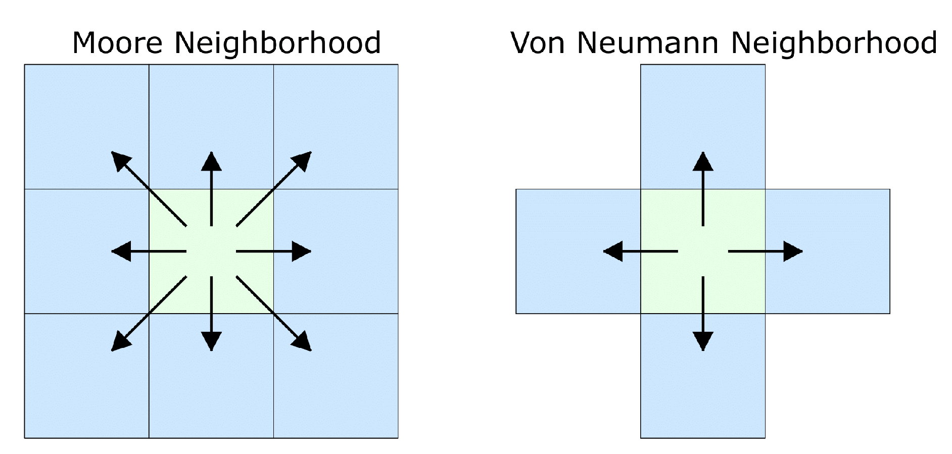
Figure 2.
Motility probability structure and directional validation of chemotactic flux. Subfigure 2a shows the Von Neumann neighborhood and associated movement probabilities. Subfigure 2b validates that the chemotactic flux field points toward the source, consistent with the model in Eq. 2.1.
Figure 2.
Motility probability structure and directional validation of chemotactic flux. Subfigure 2a shows the Von Neumann neighborhood and associated movement probabilities. Subfigure 2b validates that the chemotactic flux field points toward the source, consistent with the model in Eq. 2.1.
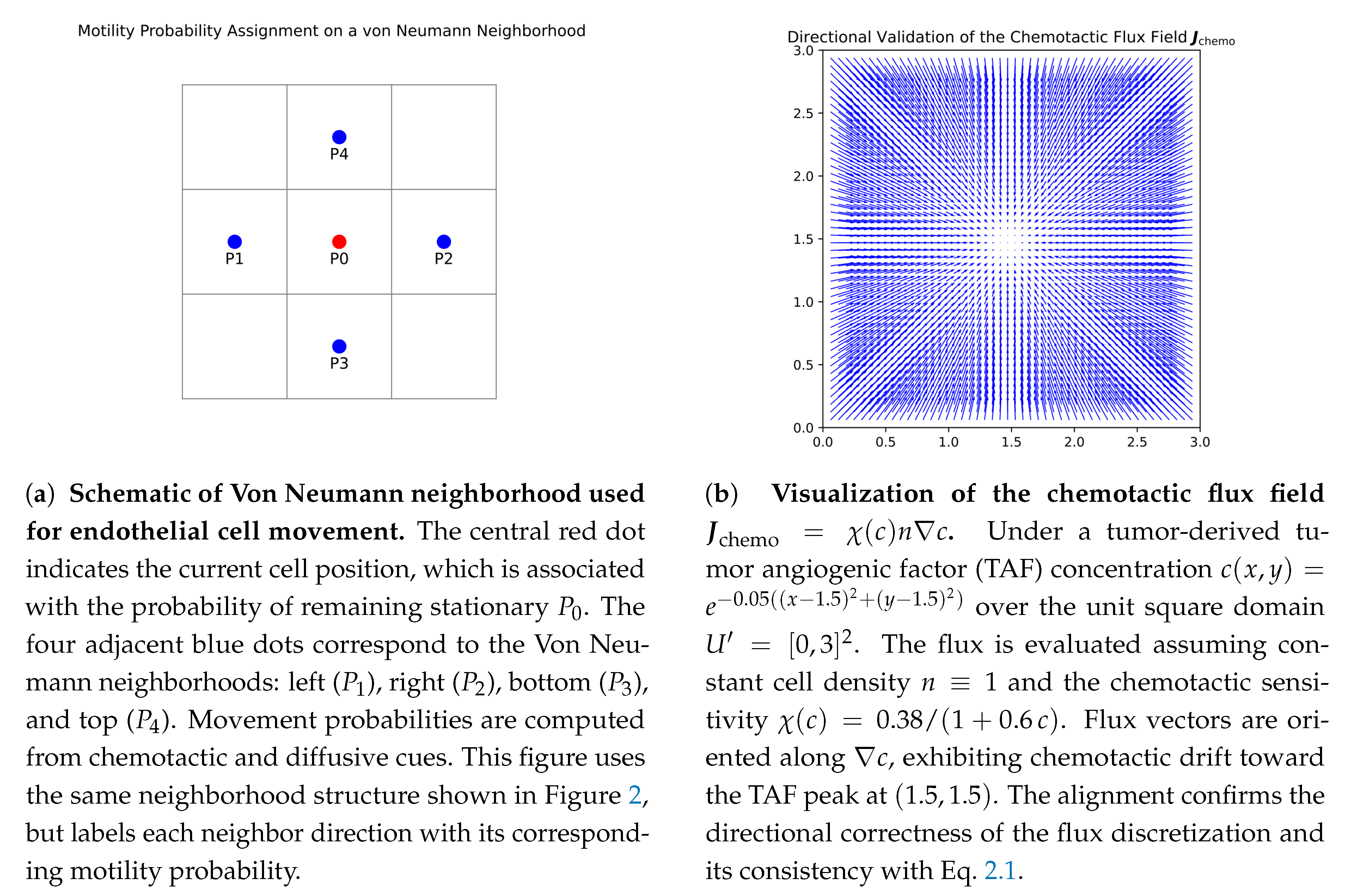
Figure 3.
A simulation shows how blood vessels form at s when the TAF concentration field is . Left: vessel sprouts exhibit a brush-border effect characterized by dense branching near the tumor-aligned boundary at . Right: traveling wave profiles of tip and vessel densities, obtained by counting horizontal vessels and tips across y-slices of the domain . The observed wave-like propagation and steady-state patterns reproduce key analytical predictions of angiogenesis models.
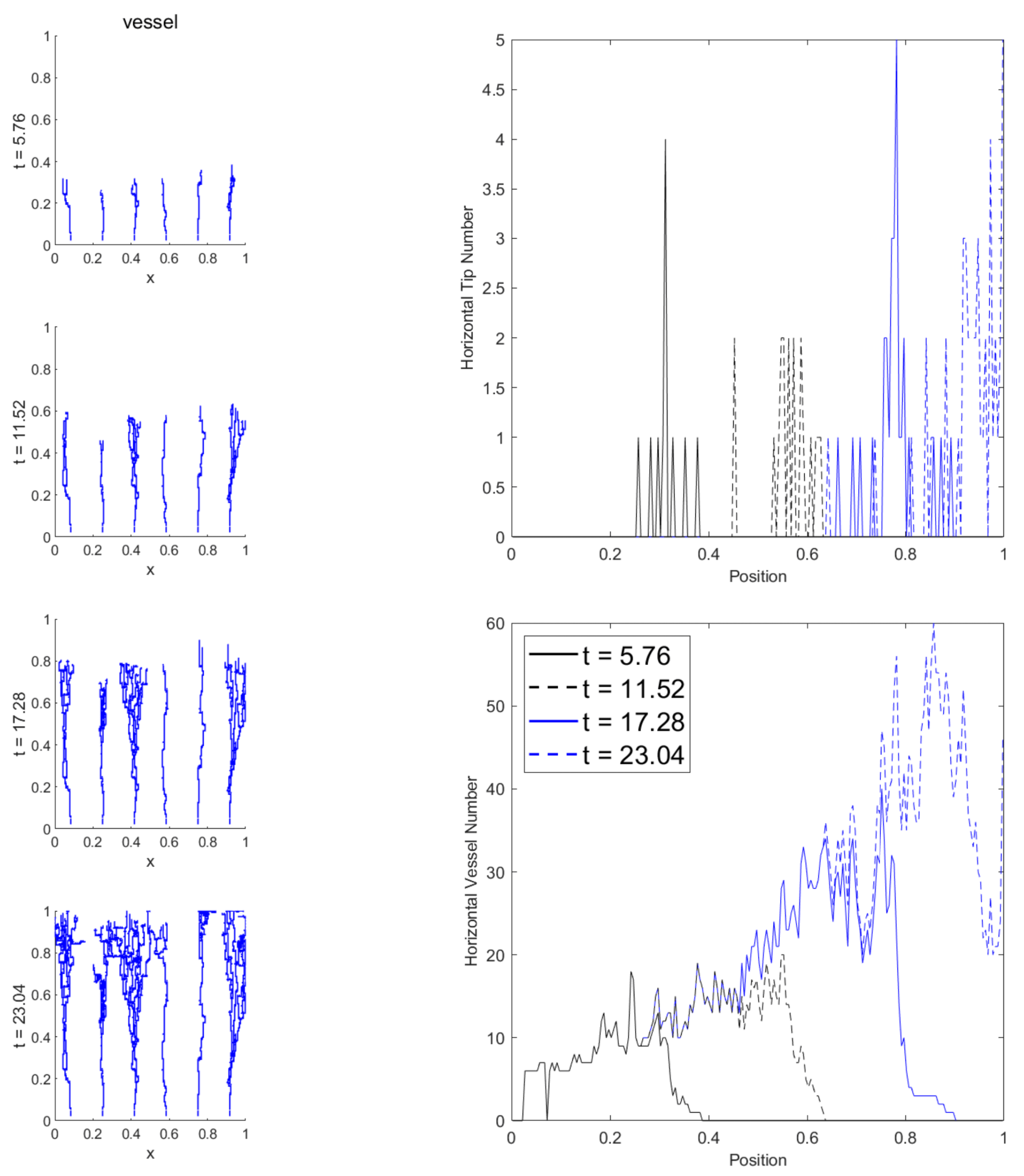
Figure 4.
Tumor-induced angiogenesis. In the early stages of tumor development, the tumor expands exponentially, leading to hypoxia in the tumor core. Subsequently, hypoxic cells release TAF, which diffuses to the surrounding tissues, forming a TAF gradient, thereby inducing angiogenesis in the hypoxic area.
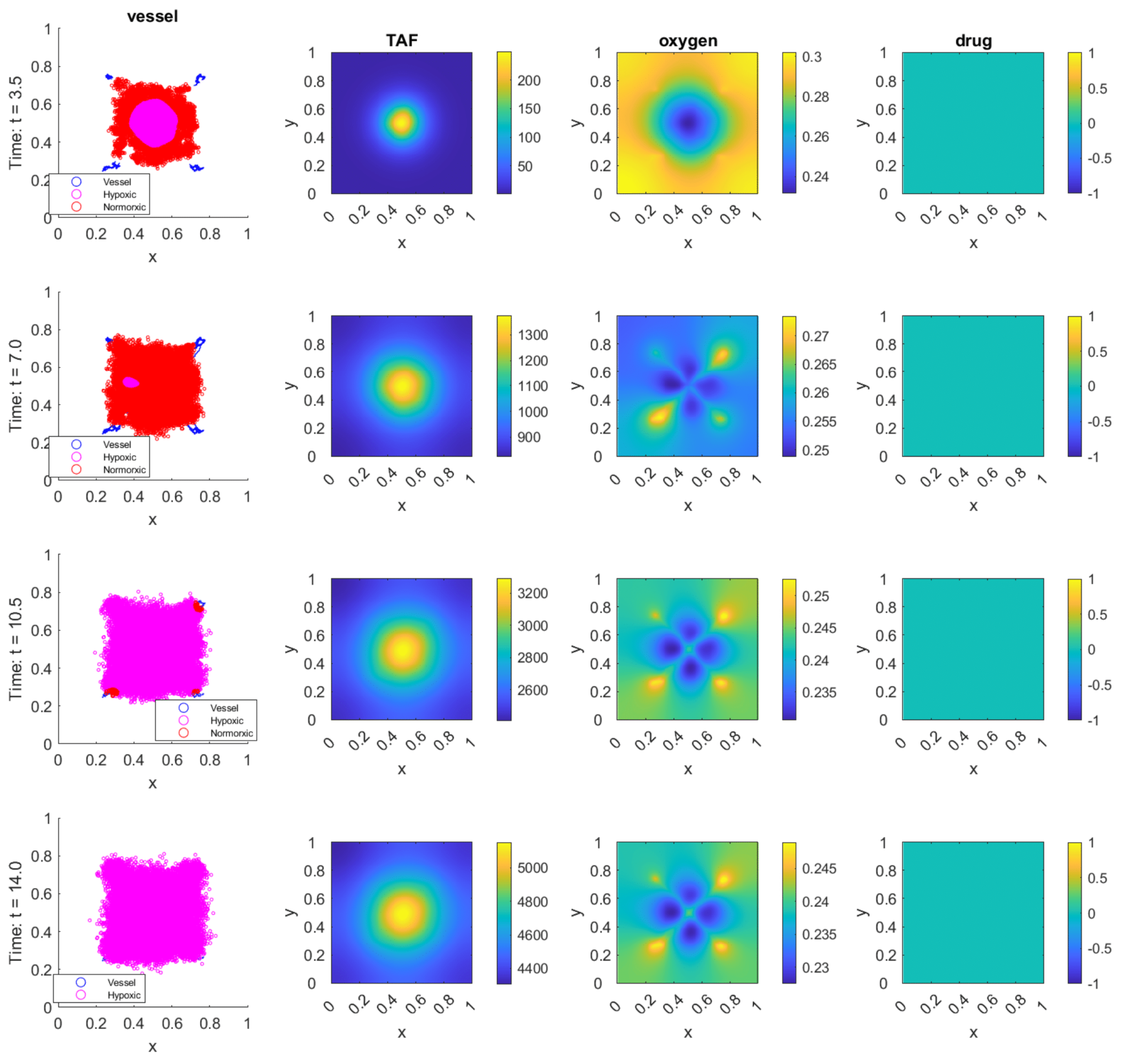
Figure 5.
Tumor dynamics under vascular regulation. Initially, exponential growth induces hypoxia, triggering TAF secretion and angiogenesis (avascular → vascular phase). The different oxygen consumption rates between cell types cause temporary fluctuations in normoxic and hypoxic cell populations, since normoxic cells consume oxygen quickly to create hypoxia, while hypoxic cells consume less and restore normoxia. These population oscillations continue until an oxygen supply-consumption equilibrium, which results in a hypoxia-dominated tumor microenvironment (TME).
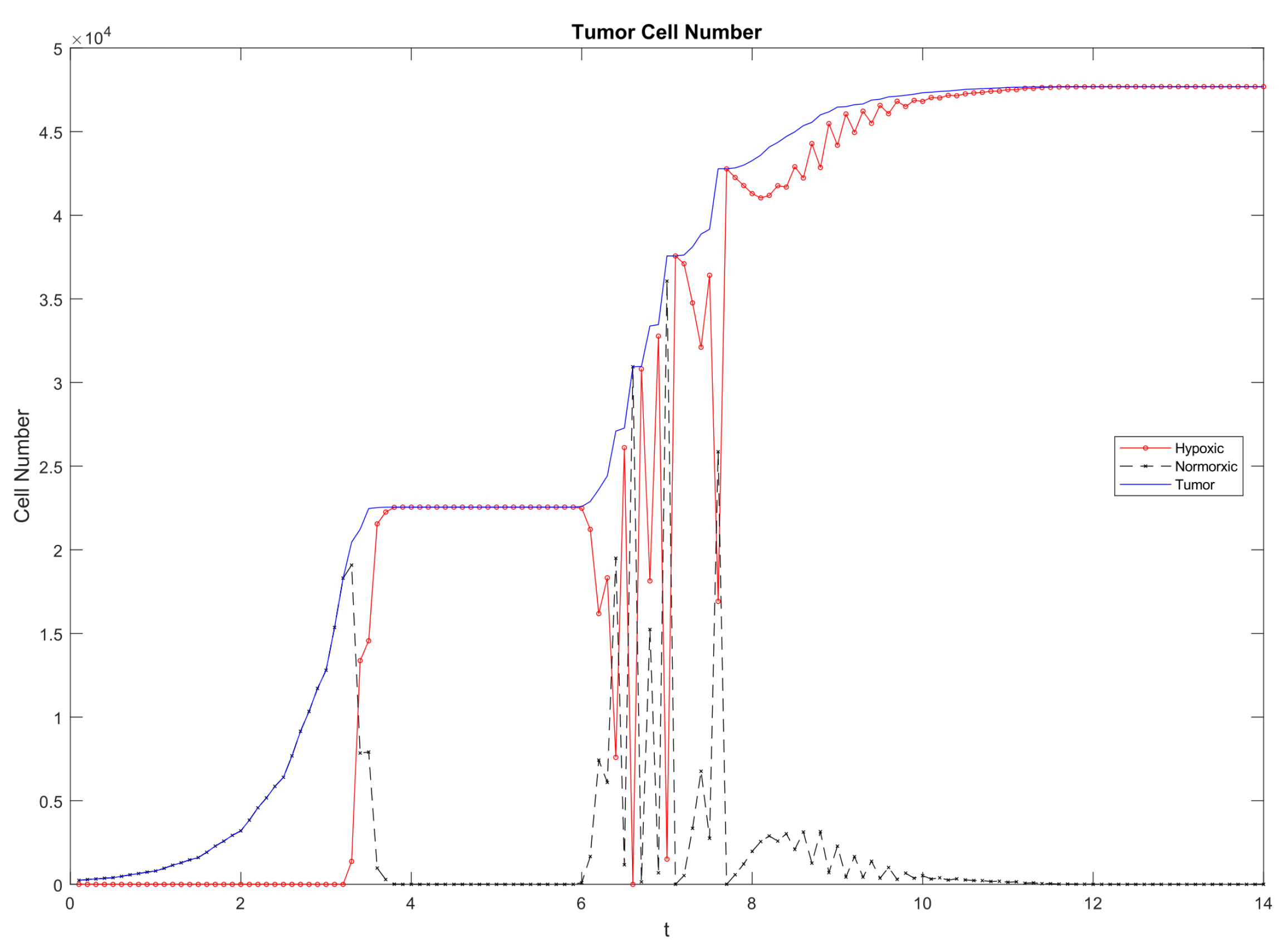
Figure 6.
Baseline therapy response in the absence of resistance. All tumor cells are initially drug-sensitive, with a death threshold , repair rate , and no mutational events. The initial population () is randomly distributed in the domain center with radius . Drug administration begins at with a constant influx rate . (a) Following the initiation of treatment, tumor cells rapidly decrease in number, leading to the alleviation of hypoxia in the TME. This promotes accelerated proliferation of the surviving tumor cells, which are predominantly normoxic. As the tumor cells continue to expand, the normoxic cells gradually transition into hypoxic cells and are eventually eliminated under the effect of the drug. (b) Linear damage increase drives cells to apoptosis, temporarily reducing density and restoring normoxia. This facilitates regrowth and synchronized division, which halves intracellular damage and regenerates the population. The system undergoes repeated oscillations in average damage, governed by the balance between accumulation and dilution.
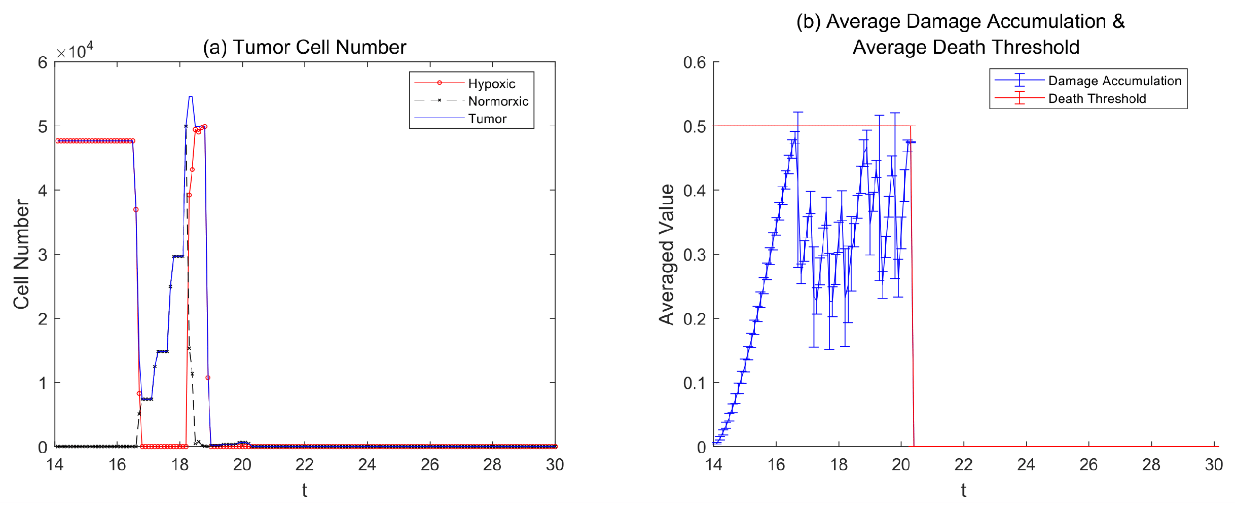
Figure 7.
Tumor dynamics in the presence of preexisting resistance. The starting population of tumor cells consists of one resistant cell () and the rest of the sensitive cells (). The drug treatment () starts at . We examine three different rates of damage clearance: , , and 1. (a) The sensitive cells die when the clearance rate is , but the resistant cells survive. This results in sustained oscillations in population size, tumor composition, and average damage because of damage-dilution cycling. (b) When the clearance rate is , sensitive cells first die in large numbers, and then resistant cells take over the population until it reaches the carrying capacity. Subsequently, both average damage levels and tumor population size stabilize, with damage remaining below the threshold while the population maintains complete resistance to therapy. (c) The maximum clearance rate of results in complete repair, which eliminates effects, thus enabling survival of both cell types and leading to treatment failure.
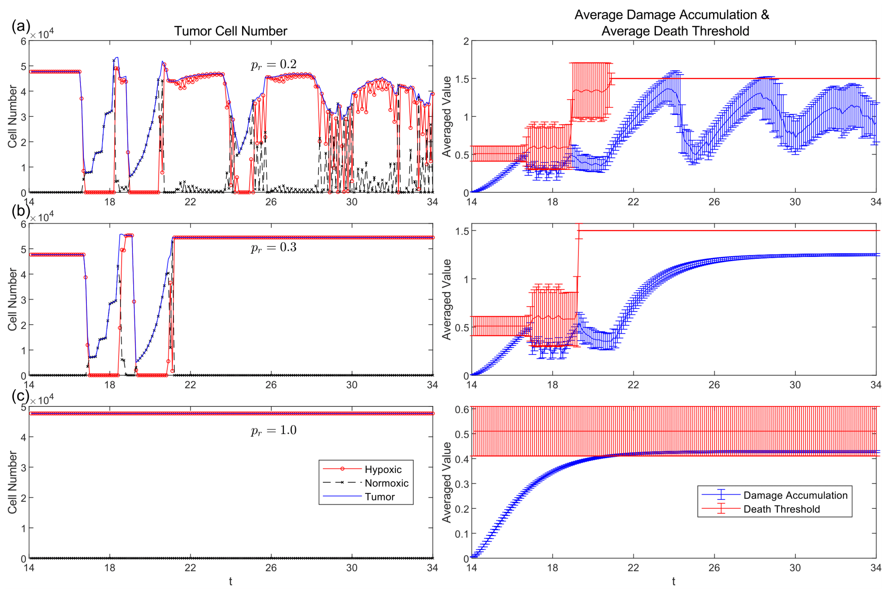
Figure 8.
Spatial distributions of normoxic and hypoxic tumor cells under preexisting resistance. The initial tumor population contains resistant cells (). We evaluate cell localization patterns under three clearance rates (, , and 1). At low clearance, resistant cells cluster near vasculature, where elevated oxygen availability supports proliferation and damage dilution, forming "vascular sanctuaries." As clearance increases, the spatial bias weakens, and tumor cells distribute more uniformly across the domain, reflecting diminished spatial selection pressures and reduced therapeutic efficacy.
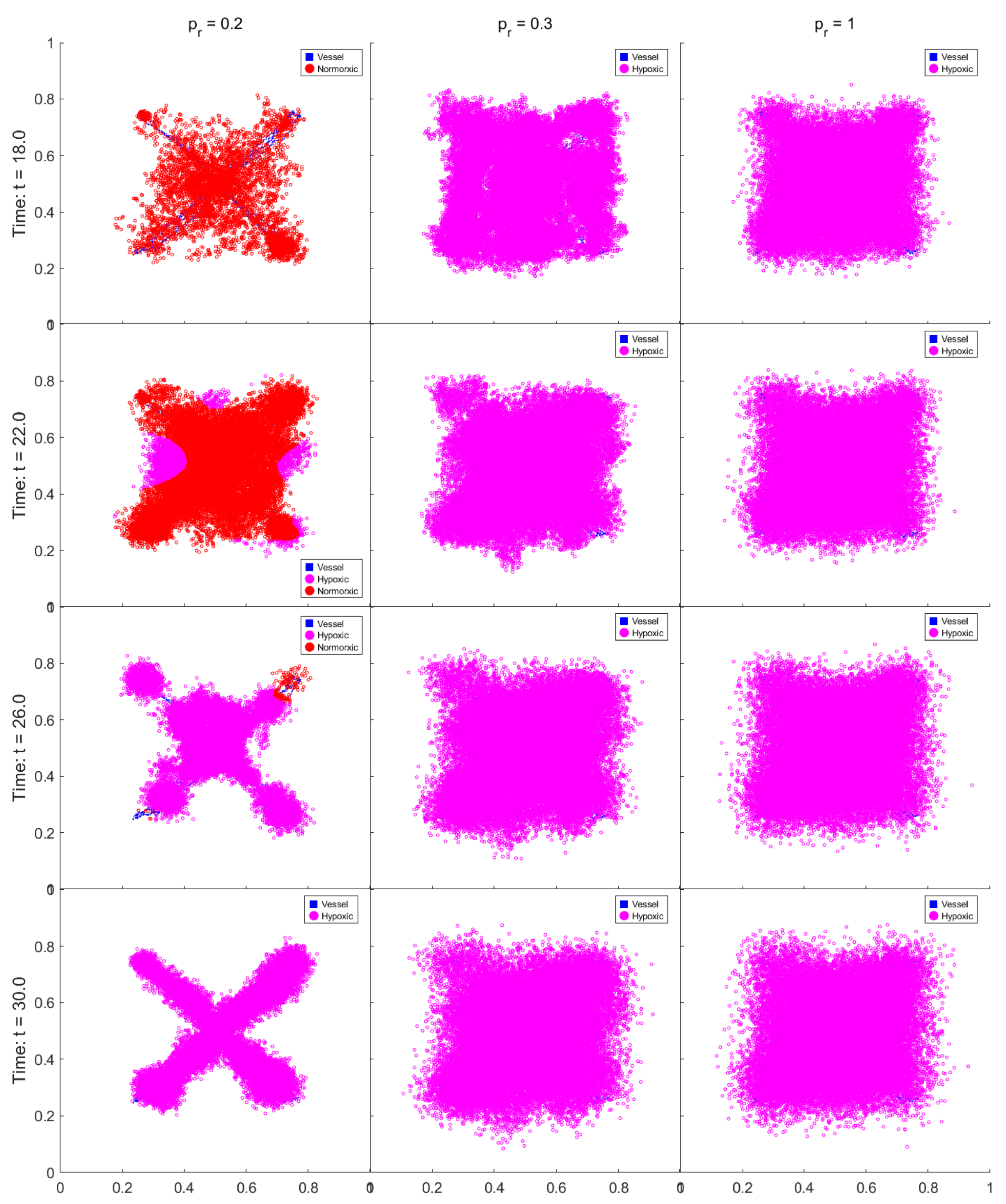
Figure 9.
Tumor dynamics under spontaneous mutation rates of , , , . (a, b, c) Tumors that have develop resistance by experiencing repeated population reduction followed by population rebounds. Two types of mass death events occur: (i) when average damage approaches the lethal threshold with minimal intercellular variation, leading to synchronized apoptosis; (ii) when substantial damage heterogeneity causes the upper tail to exceed the average death threshold, eliminating the most vulnerable cells. Surviving populations are increasingly resistant due to selective pressure. Tumors reach a quasi-stable phase at reduced carrying capacity compared to pretreatment levels. The quasi-stable phase is characterized by dampened oscillations in tumor cell counts and composition, with small-scale death events that further raise resistance through continued selection. (d) In contrast, for , insufficient mutation fails to sustain resistance, and tumors are eradicated after several treatment cycles.
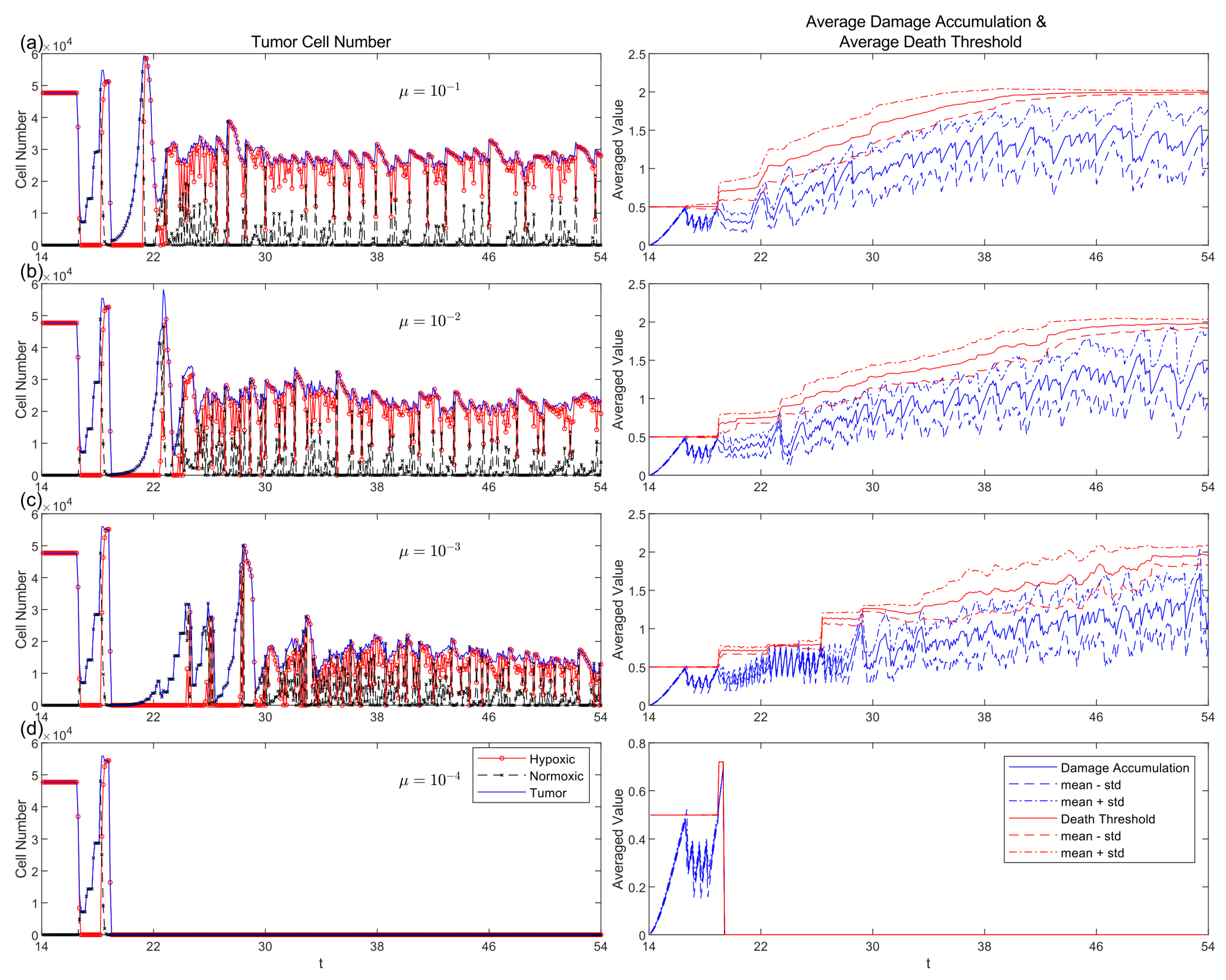
Figure 10.
Distributions of oxygen consumption along with proliferation rate exhibit temporal changes when mutation rates increase. (d) Both traits remain narrowly distributed around their starting values ( and ) when mutation rates are low at (), which indicates minimal phenotypic diversification and no emergence of resistance. (a, b, c) When increases from to the evolutionary patterns start to show up. At , the distributions of both traits begin to broaden. Oxygen consumption transitions from a unimodal to a dispersed, multimodal distribution. Directional selection becomes apparent because the unimodal distribution of the proliferation increasingly favors elevated trait values.
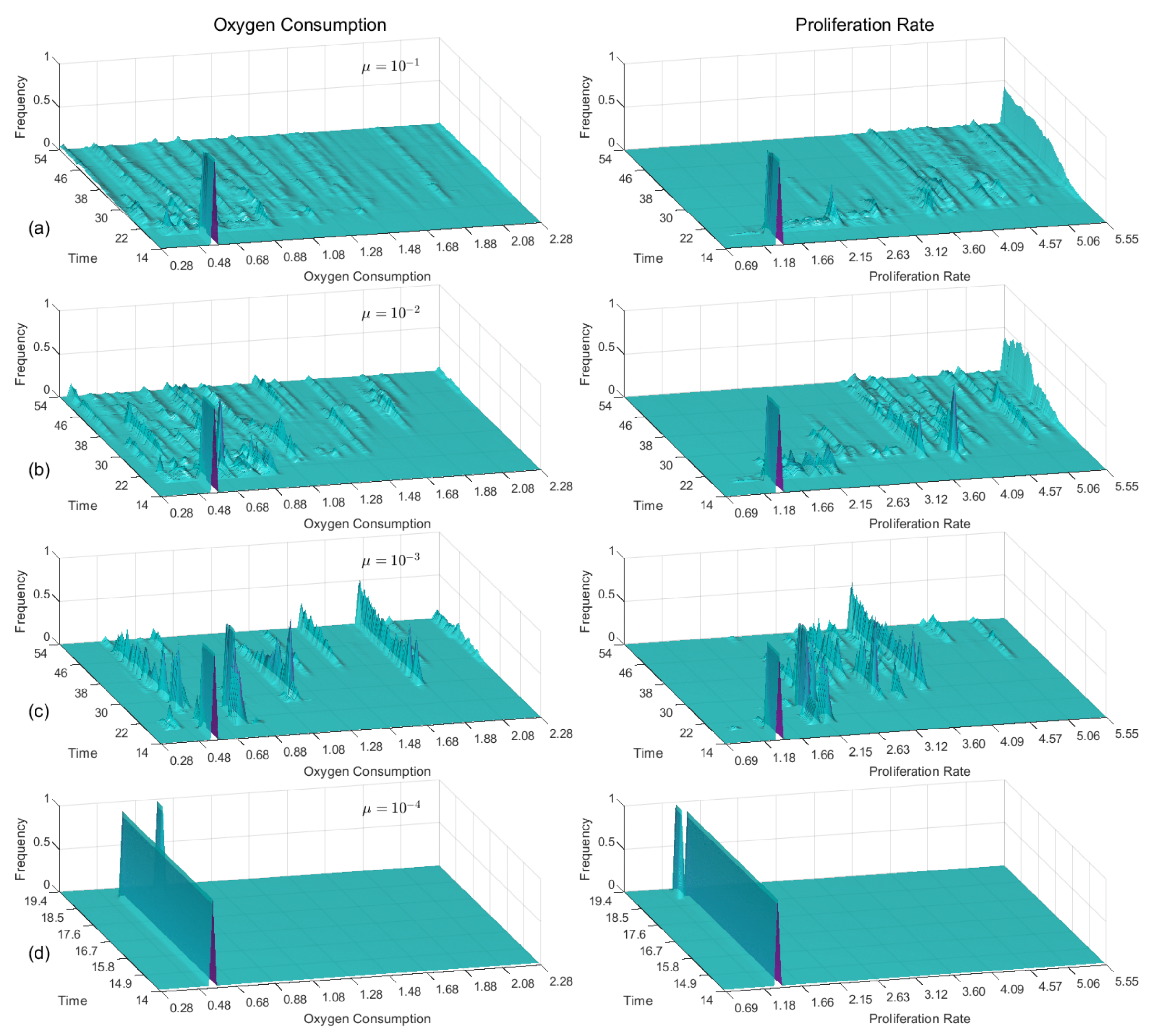
Figure 11.
The spatial distribution of cell proliferation rates under three spontaneous mutation rates: . The color bar indicates local proliferation trait values. Higher mutation rates promote fast-proliferating cells to spread throughout the population earlier in time. A direct comparison with Figure 12 shows how areas with high proliferation traits match with areas that have high resistance traits, thus demonstrating their coupled selection during evolution.
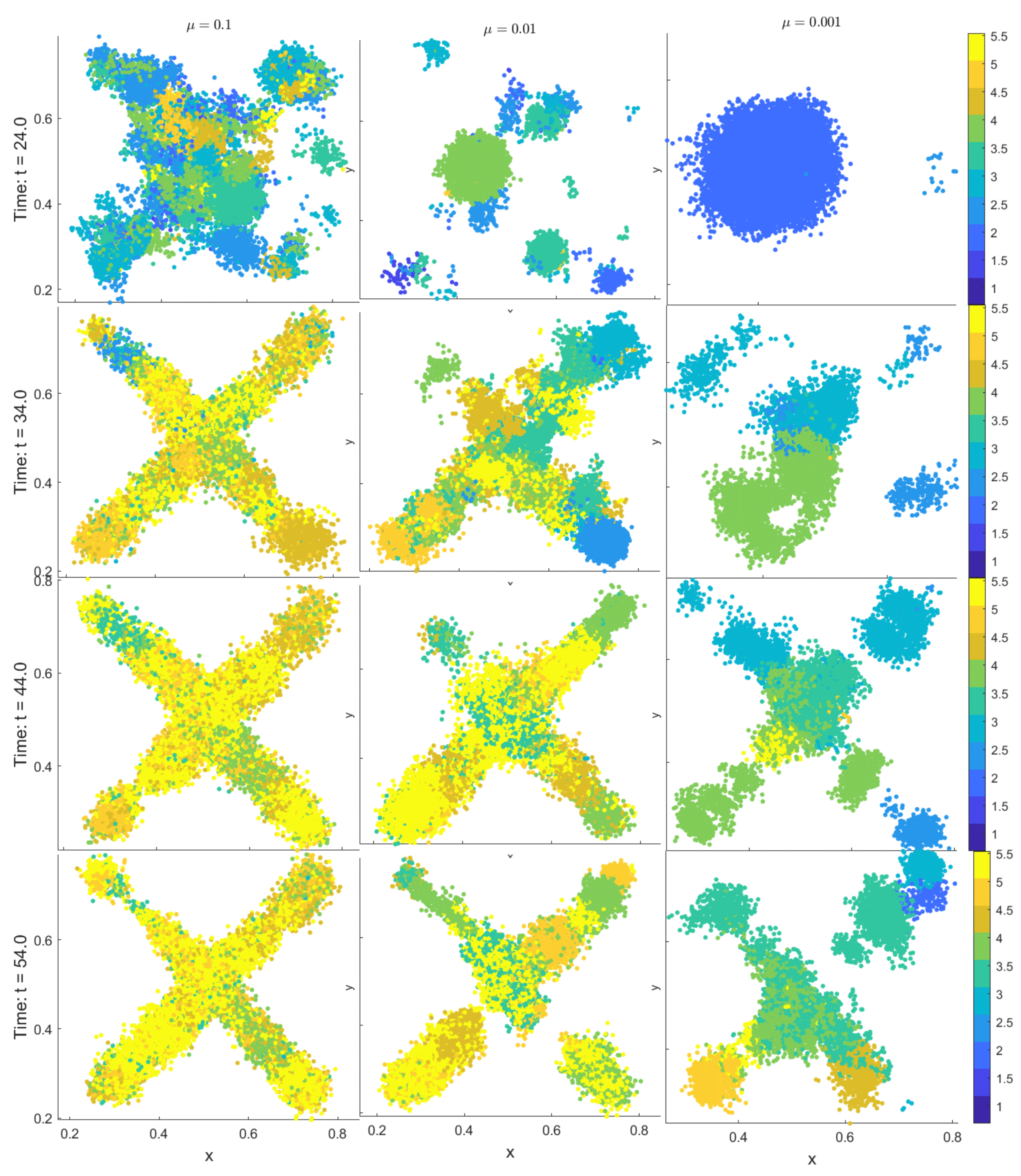
Figure 12.
The spatial patterns of resistance trait appear in three different mutation rates . The color bar indicates local resistance trait values. The presence of high mutation rates enables resistant subpopulations to appear earlier and expand faster. A direct comparison with Figure 11 demonstrates that resistance frequently matches the locations where high proliferation occurs, which supports the simultaneous selection of both traits and their joint evolutionary development.
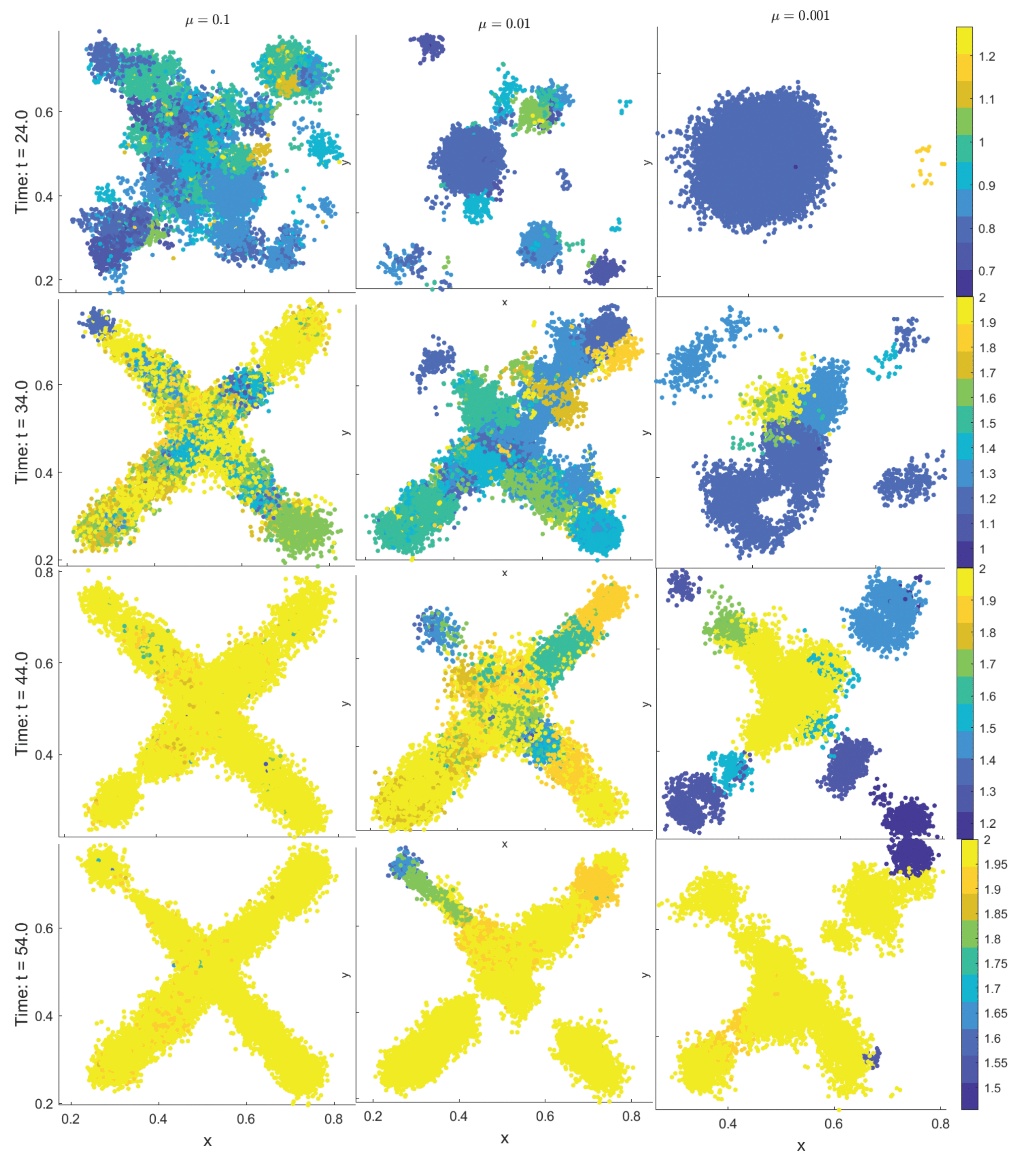

Table 1.
Mechanisms encoded in each partial differential equation (PDE) for endothelial cells n, tumor angiogenic factor (TAF) c, drug d, and oxygen o. Diffusion coefficients are denoted by , decay rates by , uptake rates by or , and source terms by or .
Table 1.
Mechanisms encoded in each partial differential equation (PDE) for endothelial cells n, tumor angiogenic factor (TAF) c, drug d, and oxygen o. Diffusion coefficients are denoted by , decay rates by , uptake rates by or , and source terms by or .
| Field | Diffusion | Decay | Uptake | Supply |
|---|---|---|---|---|
| n | None | None | None | |
| c | from hypoxic cells | |||
| d | at vessels | |||
| o |
Table 2.
Characteristic quantities used for non-dimensionalization.
| Symbol | Quantity | Rationale |
|---|---|---|
| L | Length | Spatial extent of parent vessel to tumor distance |
| Time | Typical diffusion timescale / cell cycle duration | |
| , , , | Field concentrations | Normalization of PDE variables |
Table 3.
Summary of all parameters used in the model, grouped by type: PDE system, agent-based model (ABM), and non-dimensionalization. This table provides an overview of the variables and their modeling roles. For specific numerical values (dimensional and non-dimensional) and their units, refer to Table 4.
| Parameter | Meaning |
|---|---|
| PDE-related parameters | |
| Diffusion coefficients of endothelial cells (n), TAF (c), drug (d), and oxygen (o) | |
| Chemotactic sensitivity coefficient | |
| Saturation parameter for chemotaxis | |
| Natural decay rates of TAF, drug, and oxygen, respectively | |
| Cellular uptake rates of drug and oxygen | |
| Vessel supply rates of drug and oxygen | |
| TAF production rate by hypoxic cells and uptake rate by endothelial cells | |
| Indicator functions for tumor agents and vessel locations | |
| ABM-related parameters | |
| , , , , | Sets of all tumor cells, normoxic tumor cells, hypoxic tumor cells, vessel cells, and endothelial tip cells at time t |
| Angiogenic network at time t | |
| , | Lineage identifiers for tumor and endothelial tip cells |
| , , | Spatial coordinates of agents , , at time t |
| , , , , , | Local oxygen, drug level, accumulated DNA damage, death threshold, age, and maturation time for tumor cell |
| Age of endothelial tip cell | |
| Cellular radius | |
| Mutation intensity for the Poisson process | |
| DNA damage repair or clearance rate | |
| Tumor cell motility coefficient | |
| Maximum oxygen concentration | |
| Hypoxia threshold and apoptosis threshold for oxygen concentration | |
| Probabilities of endothelial cell remaining stationary or moving left, right, down, or up | |
| Minimum age required for tip branching | |
| Branching intensity coefficient | |
| Death thresholds for sensitive and resistant tumor cells | |
| Multiplicative factor defining resistance death threshold () | |
| Tumor cell cycle duration | |
| Proliferation rate of normoxic tumor cells | |
| Crowding threshold above which proliferation is suppressed | |
| Treatment-on and drug holiday durations | |
| PDE-related parameters | |
| Non-dimensionalization parameters | |
| L | Characteristic length scale |
| Characteristic time scale | |
| Reference field concentrations used for normalization | |
Table 4.
The table presents model parameters which include physical (dimensional) values (D-values) in SI units together with their corresponding non-dimensional values (ND-values) and their sources or justifications. Non-dimensionalization based on characteristic length (L), time scale (), and concentration (). The parameters labeled “scaled” or “calibrated” were selected to attain numerical stability together with biological realism in situations without available empirical data. For a complete description of all parameters and their modeling roles, see Table 3.
| Parameter | Description | D-value (SI units) | ND-value | Source / Justification |
|---|---|---|---|---|
| Spatial discretization | (n/a) | 0.005 | Calculated | |
| Temporal discretization | (n/a) | 0.01 | Stability constraint | |
| Cellular influence radius | 0.005 | [48] | ||
| TAF diffusion coefficient | 0.12 | [49,50] | ||
| TAF decay rate | 0.002 | [29] | ||
| TAF production rate | [51] | |||
| TAF uptake rate | (n/a, nondimensionalized) | 0.1 | [52] | |
| Drug diffusion coefficient | (scaled) | 0.5 | Modeling choice | |
| Drug decay rate | (scaled) | 0.01 | [24] | |
| Drug uptake rate | (scaled) | 0.5 | [24] | |
| Drug supply rate | (scaled) | 2 | [24] | |
| Damage clearance rate | (scaled) | 0.2 | [24] | |
| Oxygen diffusion coefficient | 0.64 | [53] | ||
| Oxygen decay rate | 0.025 | [54] | ||
| Oxygen uptake rate | 34.39 | [24] | ||
| Oxygen supply rate | (calibrated) | 3.5 | Calibrated for model consistency | |
| Tumor motility intensity | (modeling choice) | 0.01 | Modeling choice | |
| Maximum oxygen concentration | 1 | [51] | ||
| Hypoxia threshold | (threshold setting) | 0.25 | [51] | |
| Apoptosis threshold | (threshold setting) | 0.05 | [51] | |
| Endothelial diffusion coefficient | [52] | |||
| Chemotaxis coefficient | 0.38 | [52] | ||
| Chemotaxis saturation parameter | (scaled) | 0.6 | [52] | |
| Branching age threshold | (scaled) | 0.5 | [52] | |
| Branching intensity coefficient | (scaled) | 1 | [25] | |
| Death threshold (sensitive cells) | (scaled) | 0.5 | [24] | |
| Death threshold ratio (resistant cells) | [55] | |||
| Cell cycle duration | 0.56–0.69 | [56,57,58,59,60,61] | ||
| Proliferation rate | Derived from | 1.0082–1.2323 | Derived | |
| Maximum neighbor cell count | (modeling choice) | 10 | [25] |
Table 5.
Summary of seven iso-dosed treatment strategies evaluated across four spontaneous mutation rates () and a preexisting resistance scenario. Each treatment cycle comprises alternating "on" and "off" periods of drug administration. Continuous regimens (Treatments 5–7) vary in dose intensity, while pulsed regimens (Treatments 1–4) vary in treatment duration but maintain a constant total dose per cycle. A symbol denotes successful tumor elimination, while indicates treatment failure. Co-dependence on mutation rate, resistance architecture, and regimen type is evident across the outcome matrix.
| Treatment | strategy | preexisting | |||||||
|---|---|---|---|---|---|---|---|---|---|
| 1 | 10 | 40 | 10 | pulsed | |||||
| 2 | 20 | 30 | 5 | pulsed | |||||
| 3 | 30 | 20 | pulsed | ||||||
| 4 | 40 | 10 | pulsed | ||||||
| 5 | 50 | 0 | 2 | continuous | |||||
| 6 | 50 | 0 | 5 | continuous | |||||
| 7 | 50 | 0 | 10 | continuous |
Disclaimer/Publisher’s Note: The statements, opinions and data contained in all publications are solely those of the individual author(s) and contributor(s) and not of MDPI and/or the editor(s). MDPI and/or the editor(s) disclaim responsibility for any injury to people or property resulting from any ideas, methods, instructions or products referred to in the content. |
© 2025 by the authors. Licensee MDPI, Basel, Switzerland. This article is an open access article distributed under the terms and conditions of the Creative Commons Attribution (CC BY) license (http://creativecommons.org/licenses/by/4.0/).
Copyright: This open access article is published under a Creative Commons CC BY 4.0 license, which permit the free download, distribution, and reuse, provided that the author and preprint are cited in any reuse.


