
Submitted:
04 August 2025
Posted:
06 August 2025
You are already at the latest version
Abstract
This study examines the drivers of food expenditure among 163,268 Filipino households using data from the PSA and advanced statistical techniques. Results indicate that although many households are high-income, they spend relatively less on food per member. Principal Component Analysis, dominant income sources such as retail, transport, farming, and remittances were identified. Furthermore, spatial clustering reveals that Leyte and Bohol exhibit the highest food spending. Notably, rural households spend more on food and have higher per capita income than urban households. Allocation of meat and bread represents the largest shares of food expenditure. Significantly, factors such as household size, income, and rural-urban status show strong nonlinear associations with food insecurity. Lastly, Engel’s curve supports that food is a necessity, with wealthier households allocating more to food consumed outside the home. Future research should incorporate finer geographic detail, nutritional measures, and longitudinal insights to enhance the robustness of the analysis.
Keywords:
food expenditure
; household income
; food insecurity
; spatial analysis
1. Introduction
Understanding the dynamics of household income and food expenditure is fundamental to shaping effective social, agricultural, and economic policies. In the Philippines, food constitutes the largest component of household consumption, accounting for the largest expenditure share in 2021 at 57.2 percent, consistent with findings from previous survey rounds [8]. This trend reinforces Engel’s Law, which states that as income rises, the proportion of income spent on food declines, even if total food expenditure increases. A deeper understanding of how food spending varies with income, geography, and household characteristics can help inform policies that aim to enhance food security and reduce poverty.
Food is a fundamental necessity and constitutes a daily expenditure for most households. In both developed and developing countries, the share of household income spent on food serves as a key indicator of economic well-being and food security. Low-income consumers spend a large share of their PCE on food, leaving less income for other essential items such as health care, housing, education, and fuel [17]. However, the Philippines, like other countries in the world, has tried to find solutions through the conduct of research and the implementation of various agricultural and nutrition programs aimed at increasing food production [10]. This program aims in ensuring food security locally, but as population increases, food expenditure tends to grow as well. This is evident in the 2021 Consumer Finance Survey of Bangko Sentral ng Pilipinas [5], stating that spending patterns of households in 2021 revealed that food and beverages consumed at home accounted for the largest expenditure share at 55.4 percent, consistent with findings from previous survey rounds. For non-food items, housing and utilities accounted for 10.6 percent, while transportation took up 7.2 percent of the budget. This spending distribution underscores the importance of government price management for essential goods and services.
The Family Income and Expenditure Survey (FIES) conducted by the Philippine Statistics Authority (PSA) provides a nationally representative dataset that captures detailed income and spending behaviors across diverse population groups. The 2023 FIES iteration, which incorporates updated sampling frames and geo-tagged data collection tools, presents an opportunity to analyze current trends in food consumption and income distribution. This study leverages that data to investigate how different household characteristics, such as income level, urban–rural status, and livelihood sources, influence patterns of food spending.
Recent studies have highlighted the value of the FIES for demand estimation. Study of [19] applied the QUAIDS model to the 2018 FIES and demonstrated how income and price elasticities of food demand vary across food groups—staples like rice showing inelastic demand, while higher-income households exhibit more flexible preferences for meat, dairy, and vegetables. Similarly, [6] examined the impact of food price shocks and government programs on nutrient intake and found that policy interventions such as cash transfers can buffer poor households against food insecurity during economic disruptions.
This study builds on those foundations by employing advanced statistical methods to assess the drivers of food expenditure. It specifically investigates the role of income deciles, livelihood types (e.g., agriculture, fisheries, wage employment), urban-rural residence, and regional differences. It contributes to the growing literature on food security, income distribution, and household economics in Southeast Asia. The findings offer empirical evidence that can inform targeted government interventions, particularly in designing effective food subsidy programs, improving livelihood opportunities. Specifically, this study sought answers to the following questions:
- What are the income and food expenditure patterns among Filipino households in 2023?
- What are the dominant sources of income for Filipino households, and how do they group or cluster?
- Are food expenditures and income spatially clustered across Philippine regions?
- How do food and income patterns differ between rural and urban households?
- How is household food expenditure distributed across major food categories among Filipino households in 2023?
- What factors predict food insecurity among Filipino households?
- How do food expenditures change as income increases?
- How much of food spending is spent outside the home, and by whom?
2. Materials and Methods
2.1. Data Collection
The data used in this study consists of 163,268 households, sourced from the Philippine Statistics Authority (PSA) and accessed through the OpenStat portal. Specifically, the study utilizes the 2023 Family Income and Expenditure Survey (FIES), Volume 1, which contains nationally representative data on household income sources, food and non-food expenditures, and demographic characteristics. This dataset provides a robust foundation for analyzing patterns in food consumption and income allocation across different socioeconomic and geographic groups in the Philippines.
2.2. Statistical Analysis
The data in this study were analyzed in alignment with the outlined research objectives, using a combination of descriptive, inferential, and other appropriate statistical techniques in RStudio v4.5.1. First, income and food expenditure patterns among Filipino households in 2023 were examined using descriptive statistics, the Gini index, and Lorenz curves to assess income inequality and food expenditure distribution. To explore the dominant sources of household income and their underlying structure, Principal Component Analysis (PCA) was conducted, supported by scree plots, PCA biplots, and loading scores to interpret income clustering and dimensionality.
To evaluate the spatial clustering of food expenditures and income across Philippine regions, spatial visualizations through regional mapping were used to identify geographic disparities in food spending intensity. A spatial boundary dataset for the Philippines was obtained from the Global Administrative Areas (GADM) database [version 4.1], which provides high-resolution administrative shapefiles for global use. The shapefile archive (gadm41_PHL_shp.zip) was downloaded from the official GADM website (https://gadm.org/download_country.html). The dataset includes polygon boundaries delineating administrative regions at various levels. For this study, only Level 1 administrative units (provinces) were used to spatially aggregate food expenditure data. Additionally, the study investigated differences in income and food spending patterns between rural and urban households using the non-parametric Mann–Whitney U test, which was selected due to the violation of normality assumptions required for parametric testing.
To analyze the composition of household food spending across major food categories, the study employed descriptive compositional techniques, including ternary plots and stacked bar charts, to assess proportional food allocations. A Generalized Additive Model (GAM) was used to analyze the factors that predict food insecurity among Filipino households. Furthermore, log-log Engel curves were constructed by plotting the natural logarithm of food expenditures against the natural logarithm of total household income. Empirical Rule of Thumb (based on Engel’s Law) was used to interpret the result of the income elasticity of food. Finally, to determine how much of household food spending is spent on food consumed outside the home, and among which household groups, a beta regression model was applied, suitable for analyzing bounded proportion data.
3. Results
3.1. Income and Food Expenditure Patterns Among Filipino Households in 2023
Descriptive statistics from the 2023 Philippine Family Income and Expenditure Survey (FIES) in Table 1 revealed that the average total household income was ₱332,147.28 (SD = ₱406,065.41), with a median income of ₱241,080.00. This large difference between the mean and median reflects a positively skewed distribution, suggesting the presence of higher-income outliers. The average total household expenditure was ₱243,155.00 (SD = ₱193,120.45), with an average food expenditure of ₱101,708.00 (SD = ₱69,317.68). The mean per capita income (RPCINC) was ₱5.49 (SD = ₱5.01), and the average household size was 5.49 people (SD = 1.91).
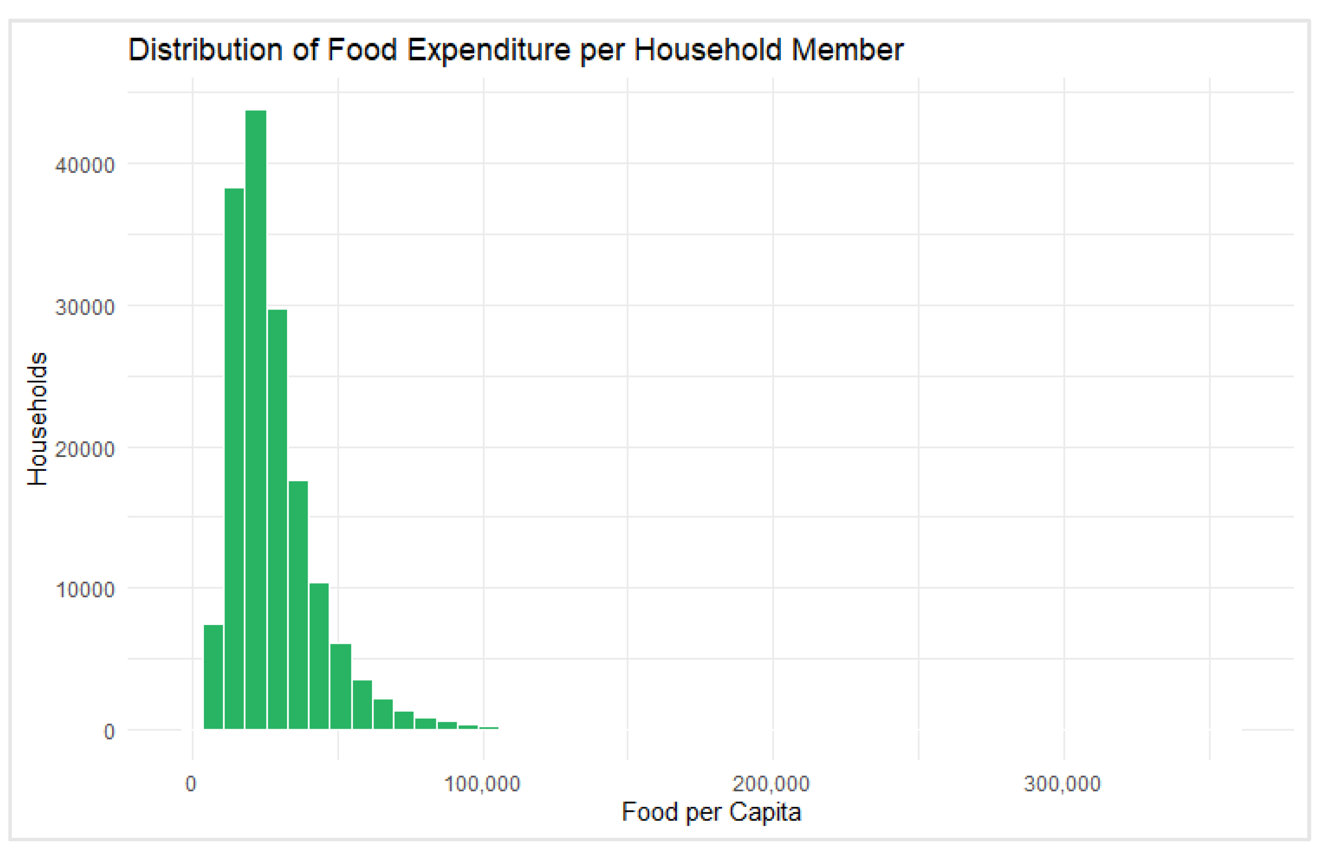
The distribution of food expenditure per household member, visualized in [Figure 2] (Histogram), shows a strong right skew, indicating that while most households spend relatively low amounts on food per member, a small number of households have disproportionately high food expenditures. While the Lorenz Curve for food expenditure in [Figure 1] indicates moderate inequality in food spending among households. The Gini coefficient for food expenditure in Table 2 was 0.277, which is lower than that of total income (Gini = 0.394) and per capita income (Gini = 0.302), implying that food expenditure is more evenly distributed than income among Filipino households.
Figure 1.
Lorenz Curve of Food Expenditure (FOOD) illustrates income-related inequality in food spending.
Figure 1.
Lorenz Curve of Food Expenditure (FOOD) illustrates income-related inequality in food spending.
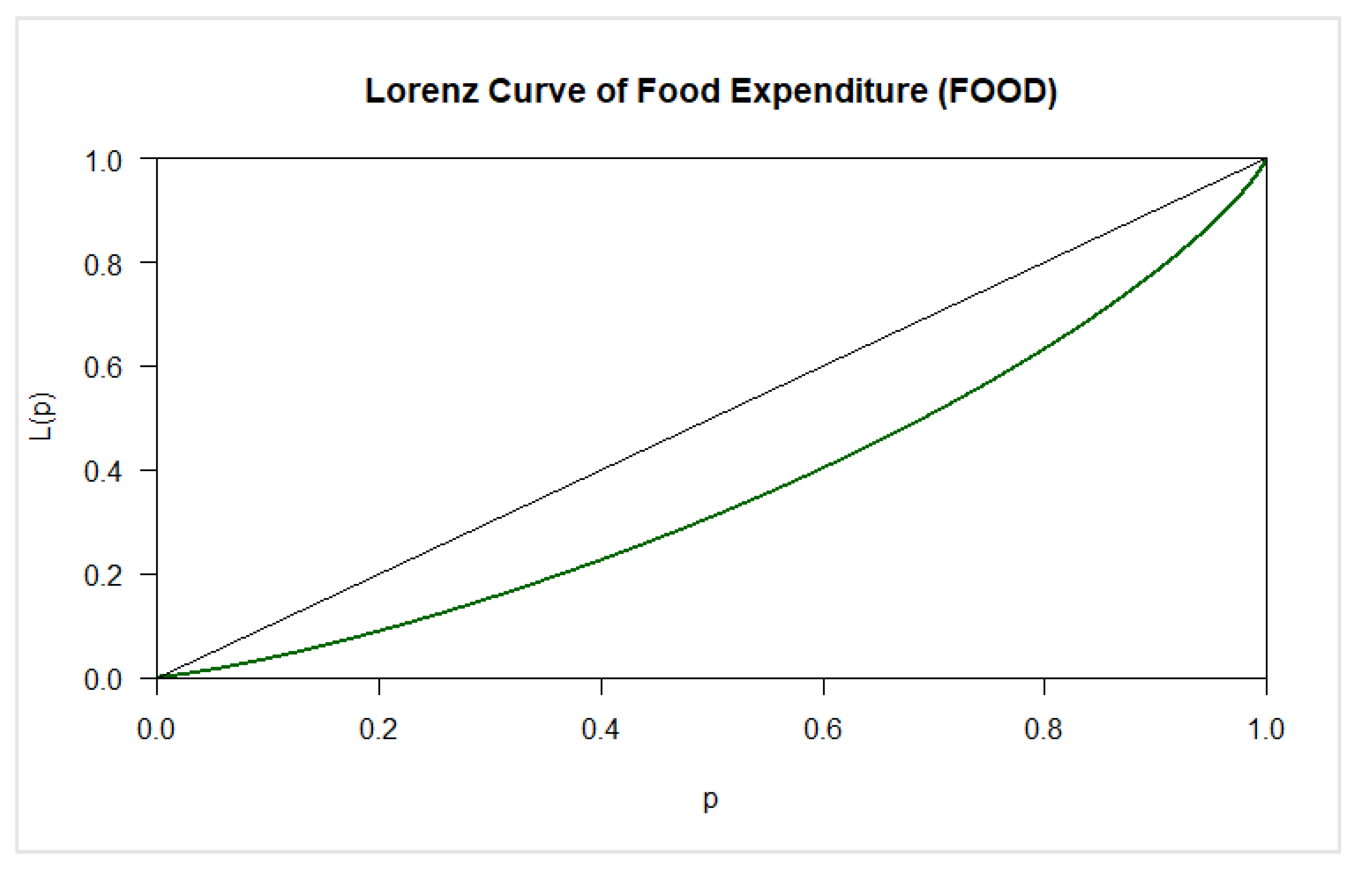
Figure 2.
Histogram showing the distribution of food expenditure per household member, highlighting skewness and concentration.
Figure 2.
Histogram showing the distribution of food expenditure per household member, highlighting skewness and concentration.
3.2. Dominant Sources of Household Income
A Principal Components Analysis (PCA) was conducted on 10 income-generating activity variables from the 2023 Family Income and Expenditure Survey (FIES), with a total sample of N = 163,268 households. Before analysis, a test of assumptions is performed. Sampling adequacy was marginally acceptable, as indicated by the Kaiser-Meyer-Olkin (KMO) measure of 0.51. Bartlett’s test of sphericity was statistically significant, χ² (45) = 15,652.99, p < .001, indicating sufficient correlations among variables to justify PCA. Based on Kaiser’s criterion (eigenvalues > 1), five components were retained, explaining 55.33% of the total variance [Figure 3]. Specifically, the first component explained 12.40%, the second 12.06%, the third 10.84%, the fourth 10.06%, and the fifth 9.97% of the variance. Table 3 revealed that in Component 1, the variables Net Retail Income (NET_RET; loading = 0.675) and Net Transport Income (NET_TRANS; loading = 0.672) had the highest positive contributions, suggesting that this dimension reflects income derived from service and retail-based economic activities and is the dominant source of household income. Component 2 was dominated by Net Other Non-Enumerated Activity Income A9 (NET_NEC_A9; 0.679) and A10 (NET_NEC_A10; 0.631), indicating a latent construct representing informal or miscellaneous economic activities. In Component 3, Net Crop, Gardening, and Livestock Income (NET_CFG; 0.638) contributed positively, while Net Fishing Income (NET_FISH; –0.661) contributed negatively, revealing contrasting agricultural and fishing-based household economies.
Component 4 showed a strong negative contribution from Net Forestry Income (NET_FOR; –0.762), along with moderate positive contributions from Net Local Paid Remittance (NET_LPR; 0.426) and Net Manufacturing Income (NET_MFG; 0.335), suggesting a divergence between forest-based and industrial-labor-related incomes. Lastly, Component 5 was mainly influenced by NET_LPR (0.610) and NET_FOR (0.575), possibly reflecting a latent contrast between remittance-based and resource-based income sources.
The PCA biplot in [Figure 4] visualizes how sectoral income sources load on the first two principal components (Dim 1 and Dim 2), which together explain 24.5% of the variance (Dim 1 = 12.4%, Dim 2 = 12.1%). Arrows pointing in the same direction and close together represent variables that are positively correlated, while orthogonal vectors indicate little to no correlation.
In the plot, NET_RET (retail) and NET_TRANS (transportation) are strongly aligned and have the longest vectors, indicating both high contribution and strong representation in the first dimension. These reflect dominant commercial income activities. In contrast, NET_CFG (Net Crop,
Gardening, and Livestock Income), NET_LPR (Net Local Paid Remittance), and NET_FISH (Net Fishing Income), associated with agriculture and fisheries, are clustered on the left side of the plot, suggesting a distinct agricultural livelihood domain that is relatively independent from commercial sectors.
Meanwhile, NET_NEC_A9 and NET_NEC_A10 (services and other economic activities) are aligned with the second dimension and form a cluster that suggests a shared informal or service-oriented economic structure. NET_FOR (forestry), while near the origin, contributes more notably in higher dimensions and appears weakly related to other variables in the 2D projection, confirming its independence seen in the loadings. Overall, the biplot supports the component structure identified in the PCA, visually confirming sectoral clustering into agriculture, services, and commerce/transport, and helps illustrate the economic segmentation among Filipino households.
3.3. Spatial Clustering of Food Expenditure in the Philippines
The spatial clustering of mean food expenditure across Philippine provinces displays clear regional groupings associated with food expenditure levels [Figure 5]. Provinces such as Cagayan, Isabela, and Southern Leyte, shaded in Indigo Purple, fall within the PHP 80,000–90,000 range, indicating relatively low food expenditure. Similarly, Quirino, Kalinga Apayao, and La Union, shaded in Noble Cause Purple, and Ilocos Sur (Acai Juice), also belong to the PHP 80,000–90,000 bracket, forming a consistent low-spending cluster in Northern Luzon. Ilocos Norte, Nueva Vizcaya (Pink Punch), and Pangasinan (Rose Violet) are likely to fall within the PHP 90,000–100,000 range.
In contrast, Leyte (Quinoline Yellow) and Bohol (Golden Ginkgo) reflect significantly higher expenditures, within the PHP 120,000 and above range, suggesting a high food expenditure cluster in Visayas. Negros Oriental (Roasted Sienna) and Eastern Samar (Fall River) follow closely, falling into the PHP 110,000–120,000 range. Meanwhile, Cebu (Chinese Purple), despite its urban profile, shows a relatively lower expenditure within the estimated PHP 80,000–90,000 range. Overall, the spatial map analysis was clustered in the Philippine Region.
3.4. Urban-Rural Household Differences in Spending Patterns
A non-parametric Wilcoxon rank-sum test (also known as the Mann–Whitney U test) [14] was conducted to compare food expenditure and income patterns between rural and urban households, as the normality assumption was violated. U Statistics are computed using the formula below:
Where: is the sum of the ranks for group 1 (Rural) and is the sum of the ranks for group 2 (Urban). Rank the number of observations from smallest to largest. The smallest value gets a rank = 1. The largest value receives a rank of . If values are tied, assign the average of the ranks for those tied values. and represent how many times values in one group precede the other in the ranking. The Mann–Whitney U test statistic is the smaller of the two:
When both and are large, and a normal distribution is used to approximate the U statistic. We calculate the Mean of U, the Standard Deviation (SD), and the Z-score (test statistic):
This Z-value is compared to the standard normal distribution to get the p-value. this is valid when both group sizes are large (typically ). A Wilcoxon rank-sum test is equivalent to the Mann–Whitney U test. The results in Table 4 revealed a statistically significant difference in food expenditure between rural (Median = ₱102,467) and urban households (Median = ₱80,700), W = 4,237,060,363, p < .001. This suggests that rural households tend to spend more on food compared to their urban counterparts. A recent study by [15] found that while urban families spend more in supermarkets, rural households shell out more overall on weekly food expenses, according to the latest findings from the 2023 National Nutrition Survey. The report, led by the Food and Nutrition Research Institute (FNRI), revealed that rural households consistently spent P100 to P500 more per week on food across various sources, including homegrown produce, traditional markets, modern groceries, and even food aid.
Similarly, a significant difference was observed in per capita income (RPCINC) between rural (Median = ₱6,000) and urban households (Median = ₱5,000), W = 3,911,776,509, p < .001. Contrary to common expectations, rural households had a slightly higher median income per capita than urban households. This means that rural households tend to have a high allocation of the budget. Additionally, study of [4] found that urban households allocate a significantly larger share of their food budget to items like meat and dairy, while rural households spend more overall but less proportionally on higher-value food categories. Overall, these findings suggest meaningful differences in food and income patterns between rural and urban areas of the Philippines, as seen in the 2023 Family Income and Expenditure Survey (FIES).
3.5. Allocation of Food Expenditure Across Major Categories
To examine the allocation of food expenditure across major categories among Filipino households, two visual analyses were conducted. focusing on five major food groups: BREAD, FISH, FRUIT, MEAT, and VEGETABLES. A ternary plot was used to explore the relative shares of major foods such as bread, meat, and fish [Figure 6]. The distribution of points shows a high density in the region between bread and meat, indicating that households tend to allocate a greater share of their food expenditures to these two categories compared to fish. Fewer households are observed near the fish apex, suggesting that fish constitutes a smaller proportion of food spending for most households. This pattern also reveals a general preference for higher expenditure on meat and bread over fish.
The average distribution of food expenditure across five major categories was also shown in a pie chart [Figure 7]. Typically, bread made up the largest portion of total food spending at 29.5%, followed by meat at 14.8%, and fish at 14.2%. Vegetables accounted for 7.2% of food expenses, while fruit had the smallest share at 4.5%. These results suggest a spending pattern that favors staple foods and protein sources (bread, meat, fish) over fruits and vegetables.
3.6. Factors Predicting Food Insecurity among Filipino Households
Generalized Additive Model (GAM) is known from mathematical theory that any multivariate function can be written as a sum and composition of univariate functions, like so:
Where; is a vector of input (independent) variables or simply the predictors. are univariate transformations of input variables (can be nonlinear). are outer functions combining those inner sums. The summation over allows an extremely flexible function form. To make the function tractable, Generalized Additive Models simplify it by removing the outer sum and enforcing a simpler function class:
Where; are smooth, univariate functions (estimated from the data). is a smooth, monotonic link function, often the identity or logit, depending on the model family. The Traditional GAM Form with Link Function is traditionally expressed using a link function that maps the expected value of the response variable to the additive predictors:
Where; is a link function, such as the logit function in logistic regression. are smooth functions estimated for each predictor . The right-hand side is additive, hence "Additive Models". When modeling the expected value of a response variable , the Generalized Additive Model (GAM) takes the form:
Where E(Y) is the expected value (mean) of the response variable. is the link function (logit) for binary outcomes. is the intercept term. are smooth (non-parametric) functions of each covariate. is the number of predictors used. In this study, a Generalized Additive Model (GAM) was estimated to assess the non-linear effects of household characteristics and net incomes on the likelihood of food insecurity using data from the 2023 Family Income and Expenditure Survey (FIES). The dependent variable was binary, indicating whether a household was food insecure (1) or food secure (0), based on whether their food expenditure ratio was below 0.30.
The model included smooth terms for continuous predictors—household size (FSIZE), real per capita income (RPCINC), net receipts from crop farming (NET_CFG), livestock and poultry (NET_LPR), fishing (NET_FISH), and forestry (NET_FOR)—as well as a parametric term for urban-rural residence (URB). The GAM model explained 27.2% of the deviance in food insecurity and had an adjusted R² of 0.229 [Table 6].
All smooth terms, except for s(NET_LPR), were statistically significant [Table 5]. The strongest nonlinear effect was observed for real per capita income (s(RPCINC); edf = 6.71, SE=0.024, χ² = 16,981.31, p < .001), indicating that income increases are associated with a sharp decline in the probability of food insecurity, especially at lower income levels. According to the study of [1], as farmers’ incomes increase, the households are more likely to have more funds to purchase food. Increasing farm income decreases the likelihood of households being food insecure and increases the likelihood of households falling outside the vulnerable group category. Furthermore, household size (s(FSIZE)) also showed a significant nonlinear effect (edf = 6.23, SE=0.014, χ² = 395.81, p < .001), indicating a nonlinear relationship with food insecurity. The predicted probability of food insecurity increased with household size, indicating that larger households are at a higher risk of experiencing food insecurity. This is evident in the study of [3] that members of large household size tend to compete for the limited resources available in the household. Large households, with younger or school-going children, also tend to be below the poverty line and vulnerable to food insecurity. These patterns are visually evident in the smooth term plots shown in [Figure 8]. Other significant predictors included net receipts from crop farming (s(NET_CFG); edf = 6.48, SE=0.006 χ² = 136.01, p < .001), indicating a modest yet significant nonlinear relationship with food insecurity. The study of [12] found that larger households with greater access to land for crop farming tended to experience lower levels of food insecurity. Notably, due to limited crop and livestock diversity, the study suggests that agricultural diversification could enhance productivity and help mitigate food insecurity. Fishing (s(NET_FISH); edf = 8.59, SE=0.005, χ² = 191.20, p < .001) and forestry (s(NET_FOR); edf = 7.93, SE=0.002, χ² = 27.04, p = .001) both show modest yet significant nonlinear associations with food insecurity. [16] emphasize that specific food coping strategies, particularly the direct consumption of caught fish, significantly reduce the likelihood of food insecurity. Similarly, [7] note that the commercialization of forest foods and other forest products, such as fuelwood, accounts for about 20% of income for rural households in developing countries. The formal forest sector also employs over 13 million people, providing income that supports food access and other basic needs.
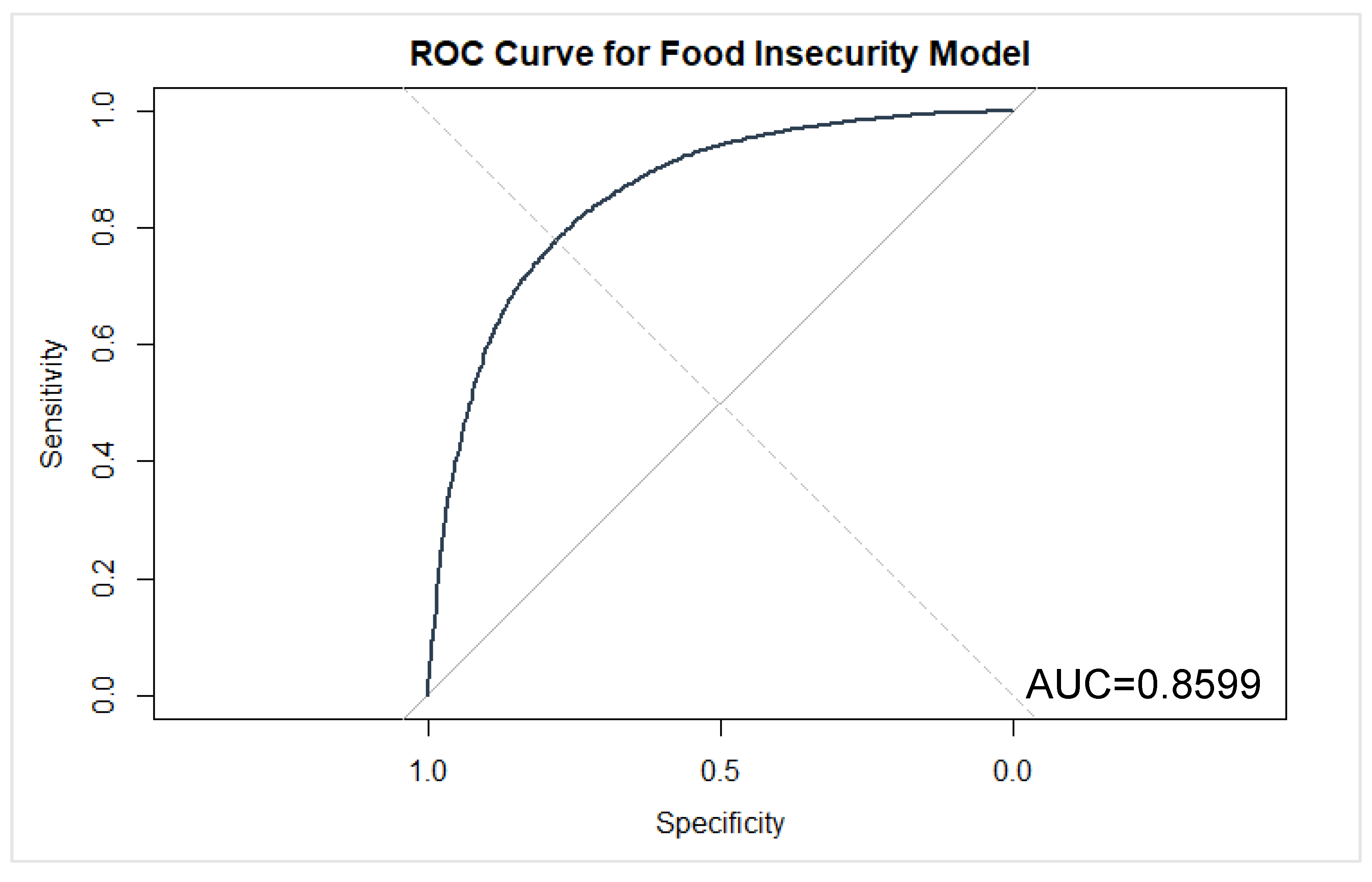
The urban-rural indicator was also a significant predictor. Residing in an urban area was associated with a lower likelihood of food insecurity (β = -0.51, SE = 0.020, z = -25.71, p < .001), indicating that rural households face higher vulnerability. A study by [11] found that rural populations had a greater prevalence of food insecurity compared to urban populations. These results contribute to this ongoing field of study by demonstrating that, rather than exclusively an urban problem, rural areas are also extensively affected by poverty and food insecurity. Model classification performance in Table 6 was strong, with an overall accuracy of 90.02% (95% CI [0.8987, 0.9016]) and an area under the ROC curve (AUC) of 0.86, indicating good discriminative ability [Figure 9]. Sensitivity was high at 97.67%, correctly identifying most food-secure households, but specificity was low at 24.93%, suggesting limited ability to correctly classify food-insecure households. The Kappa statistic was (κ=0.30), indicating fair agreement. The confusion matrix in Table 7 showed that the model correctly predicted 142,690 food-secure secure and 4,281 food-insecure households, while misclassifying 3,409 food-secure secure and 12,888 food-insecure households.

Table 5.
Generalized Additive Model Results Predicting Food Insecurity (n = 163,268).
| Predictor | Estimated df (edf) | SE | χ² / z | p-value |
| Parametric terms | ||||
| Intercept | -2.81 | 0.021 | -135.48 (z) | < .001 ** |
| URB (Urban = 1) | -0.51 | 0.020 | -25.71 (z) | < .001 ** |
| Smooth terms | ||||
| s(FSIZE) | 6.23 | 0.014 | 395.81 | < .001 ** |
| s(RPCINC) | 6.71 | 0.024 | 16,981.31 | < .001 ** |
| s(NET_CFG) | 6.48 | 0.006 | 136.01 | < .001 ** |
| s(NET_LPR) | 4.65 | 0.004 | 10.43 | .077 |
| s(NET_FISH) | 8.59 | 0.005 | 191.20 | < .001 ** |
| s(NET_FOR) | 7.93 | 0.002 | 27.04 | .001 ** |
Note: * p < .001** (Highly Significant), p < .05* (Significant), p > .05 (Not significant). SE=Std. Error.
Table 6.
Model Fit summary.
| Metric | Value |
| Adjusted R² | 0.229 |
| Deviance Explained | 0.272 |
| 95% CI for Accuracy | (0.8987, 0.9016) |
| Accuracy | 0.9002 |
| AUC (ROC) | 0.8599 |
| Sensitivity | 0.9767 |
| Specificity | 0.2493 |
| Kappa | 0.2988 |
Table 7.
Confusion Matrix and Classification Statistics for GAM Model Predicting Food Insecurity.
| Variable | Observed Food Secure (0) | Observed Food Insecure (1) |
| Predicted Secure (0) | 142,690 | 12,888 |
| Predicted Insecure (1) | 3,409 | 4,281 |
Figure 8.
Partial effect plots of smooth terms from the Generalized Additive Model (GAM) predicting food insecurity.
Figure 8.
Partial effect plots of smooth terms from the Generalized Additive Model (GAM) predicting food insecurity.
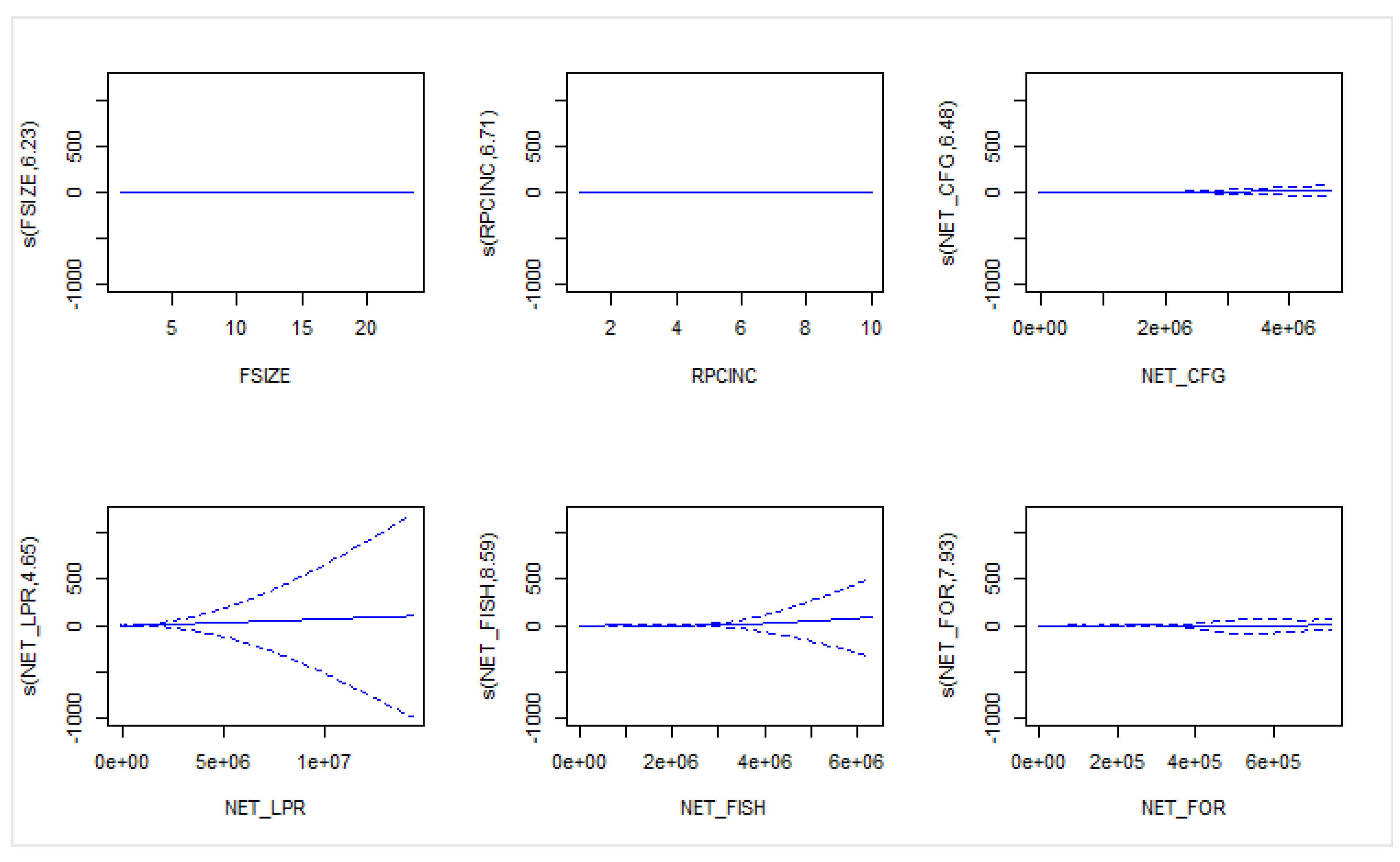
Figure 9.
Receiver Operating Characteristic (ROC) curve for the Generalized Additive Model (GAM) predicting food insecurity.
Figure 9.
Receiver Operating Characteristic (ROC) curve for the Generalized Additive Model (GAM) predicting food insecurity.
3.7. Food Expenditures: Changes When Income Increases
To determine whether food expenditures change when income increases, a linear regression analysis was first conducted using total household income as the independent variable and food expenditure as the dependent variable. This model provided a direct estimate of how much food spending increases with each additional peso of income. To better capture the proportional (percentage-based) relationship between income and food expenditure — especially since this relationship may not be strictly linear — a log-log linear regression was also performed. In this model, both total income and food expenditure were transformed using natural logarithms. This approach linearizes any power-law (non-linear) relationships and allows the slope of the regression line to be interpreted as the income elasticity of food — that is, the percentage change in food spending for a 1% change in income.
We start by modeling the raw relationship between food expenditure (FOOD) and total household income (TINC) using a basic linear regression model:
Where; is the food expenditure of the household i. is the total income of household i. is the intercept (baseline food spending when income is zero). is the change in food spending per peso increase in income, and is the error term (unexplained variation). However, this raw model assumes a constant rate of increase, which may not reflect reality. In real-world data, especially for necessities like food, spending tends to increase with income at a decreasing rate. To better capture this non-linear, diminishing growth relationship, we take the natural log of both variables, converting the model into a log-log linear regression, which is known as the log-log Engel Curve.
Where; This is the log of food expenditure. This is the log of total income. is the intercept (baseline log food spending). is the income elasticity of food (explained below) and is the error term. In a log-log model, the coefficient represents elasticity.
Based on the result in Table 8, in the simple linear regression, total household income significantly predicted food expenditures, = 0.072, SE = 0.00028, t = 252.7, p < .001, with an intercept of ₱77,880 (SE = 148.90). The model explained approximately 28.1% of the variance in food expenditure, R² = .281. Coefficient() indicates that for every additional peso in income, food expenditure increases by approximately 7.2 centavos. Furthermore, to assess income elasticity, a log-log linear regression model was estimated. The results showed that log-transformed income significantly predicted log-transformed food expenditure, = 0.580, SE = 0.00120, t = 484.2, p < .001, with an intercept of 4.177 (SE = 0.01494). This model accounted for a larger proportion of variance, R² = .589. Coefficient() shows that for every additional peso in income, food expenditure increases by approximately 58.0 pesos.
Thus, the estimated income elasticity of ε = 0.58 means that among Filipino households, food demand is income inelastic. In simple terms, when a Filipino household’s income increases by 1%, their food spending increases by only 0.58%. This indicates that food is a necessity good; Engel's law establishes that as income increases, households' demand for food increases less than proportionally [9]. This result is consistent with Engel’s Law in Table 9, which states that as a household's income rises, the proportion of income spent on food decreases, even if the total peso amount spent on food goes up. In the Philippine context, this suggests that wealthier households allocate a smaller share of their income to food compared to lower-income households, although they still spend more in absolute terms. A scatterplot of the Engel Curve, with log-log values and a fitted regression line, is presented in Figure 10, illustrating the positive but inelastic relationship between income and food expenditure.
3.8. Food Spent Outside the Home, and by Whom?
A beta regression model was fitted to examine the effect of household income, urbanicity, and household size on the proportion of food expenditure outside the home. The dependent variable (FOOD_SHARE_OUT_BETA) was transformed using the formula:
Where; is the original proportion of food spending outside the home, is the number of observations, and is the adjusted value constrained strictly between 0 and 1, necessary for beta regression. The beta regression model assumes the dependent variable and models the mean using a logit link below
Where; is the predicted average share of food spending outside the home for household i. are the regression coefficients. is the natural log of household income. = 1 if urban, 0 if rural and is the household size. Instead of modeling directly, we model the logit of , this transformation makes sure predictions stay between o and 1.
Formula above is called the logit link, it’s common when the dependent variable is a proportion. Additionally, beta regression requires . To adjust original values that might be 0 or 1, the transformation of [18] is used:
Where; is the original food share (could be 0 or 1). is the total number of observations and is the transformed value used in the model. The log-likelihood function is the heart of Maximum Likelihood Estimation (MLE). In beta regression, we assume that the dependent variable follows a Beta distribution:
Where; is the response variable (FOOD_SHARE_OUT_BETA). is the mean of the beta distribution for observation i and is the precision parameter (higher =less variance). Variance can be computed using the formula below:
Where; varies by both and ; no constant variance. , product is largest near 0.5 and smallest near 0 or 1. It reflects how much room the proportion has to vary — values near the extremes can't vary much. is the precision parameter higher means less variance, data points are tightly clustered around the mean . So, High , low means high variance (e.g., lots of different spending patterns) and Low , high means low variance (people mostly spend close to average). On the other hand, beta regression does not use traditional R². Instead, it uses McFadden’s Pseudo R²:
Where; is the log-likelihood of the fitted model. is the log-likelihood of the null model (intercept only). The log-likelihood function for a beta distribution is:
Where; is the Gamma function (generalized factorial). is the log of gamma function of precision. are the shape component of the beta distribution. are the Likelihood contribution for the observation’s actual value and are the Complementary contribution (1 minus observation). is the adjusted proportion of food expenditure outside the home. is the predicted mean from the regression model. is the precision parameter (estimated separately) and is the number of observations.
Beta regression in this study is appropriate since assumptions test shows a not normal distribution as well as there is a heteroskedasticity (variance depends on the mean) found. A beta regression was conducted to examine the association between the proportion of food expenditure spent outside the home (FOOD_SHARE_OUT_BETA) and the predictors: log household income (log_INCOME), urbanicity (URB), and household size (FSIZE). The outcome variable was transformed to lie strictly between 0 and 1 and modeled using a logit link function. Results in Table 11 indicated that the overall model was statistically significant, with a log-likelihood of 647,500 and a pseudo-R² of .1403, suggesting that approximately 14.03% of the variance in food expenditure share outside the home was explained by the predictors.
The results in Table 10 revealed that income, urban residence, and household size were statistically significant predictors of the outcome variable. Specifically, log-transformed income (log_INCOME) was positively associated with the share of food spent outside the home, =0.72, SE = 0.004, z = 169.32, p < .001, suggesting that higher-income households allocate a larger proportion of food spending outside. A study by [2] states that higher income dramatically influences household consumption behavior linked to eating out. Generally, rising per capita income increases people's demand for food prepared outside. Hence, individuals with higher incomes often dine out and spend more on outside food. Conversely, urban (URB) households spent a significantly lower proportion of food spending outside compared to rural households, =−0.50, SE = 0.005, z = -91.33, p < .001. Household size (FSIZE) also had a small but significant negative effect, =−0.026, SE = 0.001, z = -19.05, p < .001, indicating that larger households tend to spend proportionally less outside the home. A study of [13] found a statistically significant difference in consumption patterns by household size. It noted: “larger households tend to spend proportionally less outside the home,” suggesting that they are more likely to cook at home and purchase food and other goods in bulk, which reduces per-capita out-of-home spending.
The precision submodel estimated a dispersion parameter (ϕ) of 2.90 (SE = 0.014, z = 208.1, p < .001), indicating a moderate level of concentration of values around the predicted mean. This implies relatively low variability of responses around the mean food share. Quantile residuals ranged from -8.71 to 8.21 (Median = 0.44), showing acceptable dispersion and no major violations of normality or linearity. The residual pattern and distribution suggest that the assumptions of beta regression were reasonably met. No extreme heteroscedasticity or violations of the model structure were evident from the residual diagnostics.
Table 10.
Beta Regression Results Predicting Food Expenditure Share Outside the Home.
| Predictor | (Estimate) | SE | z-value | p-value |
| (Intercept) | -10.611 | 0.055 | -192.39 | p < .001 |
| log_INCOME | 0.717 | 0.004 | 169.32 | p < .001 |
| URB | -0.498 | 0.005 | -91.33 | p < .001 |
| FSIZE | -0.026 | 0.001 | -19.05 | p < .001 |
Note: * p < .001 (Highly Significant), p < .05 (Significant), p > .05 (Not significant). SE=Standard error.
Table 11.
Assumptions of the Model.
| PRECISION PARAMETER | MODEL FIT | RESIDUALS | ||||||||
| Precision (ϕ) | SE | z-value | p-value | Log Likelihood | Pseudo R² | Min | 1Q | Median | 3Q | Max |
| 2.90 | 0.014 | 208.1 | p < .001 | 647,500 | 0.1403 | -8.71 | -0.31 | 0.44 | 0.86 | 8.21 |
Note: p < .001 (Highly Significant), p < .05 (Significant), p > .05 (Not significant), SE=Standard error.
4. Discussion
This study provides a comprehensive assessment of the interplay between household income and food expenditure among Filipino households using the 2023 Family Income and Expenditure Survey (FIES). The findings reaffirm the economic principle established by Engel’s Law, highlighting that food, though essential, constitutes a smaller proportion of household budgets as income increases. This reflects broader consumption patterns in developing economies, where food remains a central but diminishing share of expenditure with rising prosperity. Importantly, the relatively equitable distribution of food spending, compared to income, underscores the prioritization of food across income groups and reflects a fundamental consumption behavior that policy frameworks must continue to protect.
The structural segmentation of income sources across Filipino households revealed distinct livelihood patterns. Households rely on diverse combinations of agricultural, commercial, and informal income streams, which reflect the geographic and occupational heterogeneity of the country. Such economic segmentation suggests that national food security and poverty alleviation programs must be more nuanced and localized, aligning with the specific income structures and vulnerabilities of each sector. Additionally, the observed spatial disparities in food expenditure across regions point to geographic inequality in food access and affordability, likely influenced by regional variations in food prices, supply chains, and economic activity. These patterns highlight the urgent need for geographically targeted policies, especially in under-resourced provinces, where food insecurity risks may be exacerbated by both income constraints and infrastructural limitations.
Differences between rural and urban households challenge long-held assumptions. While urban areas typically enjoy better access to markets and services, rural households exhibited higher food spending and slightly greater per capita income. This may be due to differences in cost structures, household sizes, or the availability of home-produced food in rural settings. However, rural households remain more vulnerable to food insecurity due to limited access to health services, infrastructure, and diverse food options. The patterns in food allocation, particularly the dominance of energy-dense but nutrient-poor staples such as bread and meat, raise questions about the quality and diversity of household diets, especially among low-income groups. Addressing food security, therefore, extends beyond affordability to include nutritional adequacy and education.
Understanding the predictors of food insecurity at the household level is crucial for effective intervention design. This study identifies critical factors such as income level, household size, and rural residence, all of which have complex, nonlinear effects on the likelihood of experiencing food insecurity. Larger households, for instance, face increased vulnerability, especially when combined with low income and dependence on unstable livelihood sources like farming or fishing. Meanwhile, the evolving patterns of food consumption such as increased spending on food outside the home among higher-income and rural households reflect shifts in consumer behavior and lifestyle. These behaviors may signal transitions in food culture and labor dynamics, warranting further attention from both researchers and policymakers.
Despite the strengths of the dataset and analytical techniques used, several limitations must be acknowledged. First, the cross-sectional nature of the FIES limits causal interpretations; while associations between variables can be established, temporal dynamics cannot. Second, the survey lacks detailed information on dietary diversity, nutritional status, or food sufficiency measures that are vital for a more holistic understanding of food security. Third, spatial analysis was limited to provincial-level aggregates, which may obscure intra-provincial disparities and urban-rural gradients within regions. Finally, reliance on self-reported data for income and expenditures may introduce recall bias or misreporting, particularly among households engaged in informal or non-monetized economic activities. Future research would benefit from incorporating longitudinal data, qualitative insights, and more granular geographic information to strengthen the evidence base for policy design.
5. Conclusions
This study aimed to explore how income, geography, and household characteristics shape food expenditure behaviors among Filipino households. Drawing on data from the 2023 Family Income and Expenditure Survey (FIES), the study employed a combination of descriptive analysis, spatial mapping, principal component analysis, generalized additive modeling, Engel curve estimation, and betaregression to address key research questions related to household income, food spending patterns, and food insecurity.
Specifically, the study sought to: (1) examine income and food expenditure patterns; (2) identify dominant sources of income and how households cluster by livelihood; (3) assess spatial clustering of income and food expenditure across Philippine regions; (4) compare rural and urban food and income dynamics; (5) describe food expenditure allocation across major food categories; (6) identify factors predicting food insecurity; (7) evaluate how food spending changes as income rises; and (8) determine which households spend more on food outside the home.
The findings showed that food expenditures are inelastic to income, confirming Engel’s Law, and that while income inequality remains high, food spending is more evenly distributed. Regional disparities in food expenditure were evident, and significant differences emerged between rural and urban households—rural families tended to spend more on food and showed higher per capita income in some cases, yet remained more vulnerable to food insecurity. Principal component analysis revealed sectoral distinctions in income sources, while generalized additive modeling identified household size, income level, and location as key predictors of food insecurity. Notably, wealthier and smaller households spent more on food consumed outside the home, though rural households exhibited a surprisingly higher proportional share.
The study contributes to the literature by integrating multidimensional methods to provide a holistic view of income and food dynamics in the Philippines. Importantly, it highlights the need for differentiated and localized food and income support programs that consider household structure, livelihood type, and spatial context. While the cross-sectional nature of the data and the lack of nutritional detail limit causal inference and dietary conclusions, the study offers a strong empirical basis for evidence-informed policymaking in food security, social protection, and rural development.
Future research should build on this foundation by incorporating longitudinal or qualitative data, expanding to more granular geographic units, and including nutritional adequacy indicators to deepen understanding of household food systems in the Philippine setting.
Supplementary Materials
The following supporting information can be downloaded at the website of this paper posted on Preprints.org.
Data Availability Statement
The data that support the findings of this study are confidential and are not publicly available due to privacy restrictions. Access to the dataset may be granted upon reasonable requests and with permission from the corresponding data owner.
Acknowledgments
The author thank the reviewers for their comments which helped to improve the presentation of this manuscript
Conflicts of Interest
The author declares no conflict of interest associated in this study.
References
- Addison, M., Ohene-Yankyera, K., Acheampong, P. P., et al. (2022). The impact of uptake of selected agricultural technologies on rice farmers’ income distribution in Ghana. Agric & Food Security, 11(2). [CrossRef]
- Ahmed, M. R. (2023). Household consumption expenditure behavior towards outside ready-made food: Evidence from Bangladesh. Heliyon, 9(e19793). [CrossRef]
- Akello, M. C., & Mwesigwa, D. (2023). Household size and household food security in Ngetta Ward, Lira City, Northern Uganda. International Journal of Developing Country Studies, 5(1), 88–109.
- Bairagi, S., Zereyesus, Y., Baruah, S., & Mohanty, S. (2022). Structural shifts in food basket composition of rural and urban Philippines: Implications for the food supply system. PLoS ONE, 17(3), e0264079. [CrossRef]
- Bangko Sentral ng Pilipinas. (2025). 2021 Consumer Finance Survey (CFS). https://www.bsp.gov.ph/SitePages/MediaAndResearch/MediaDisp.aspx?ItemId=7451.
- Briones, R. (2022). Food and nutrient intake response to food prices and government programs: Implications for the recent economic shocks. [CrossRef]
- Chamberlain, J. L., Darr, D., & Meinhold, K. (2020). Rediscovering the contributions of forests and trees to transition global food systems. Forests, 11(10), 1098. [CrossRef]
- Cigaral, I. N. (2025). BSP survey shows how Filipinos spent in moments of crisis. Philippine Daily Inquirer. https://business.inquirer.net/513337/bsp-survey-shows-how-filipinos-spent-in-moments-of-crisis.
- Cirera, X., & Masset, E. (2010). Income distribution trends and future food demand. Philosophical Transactions of the Royal Society B: Biological Sciences, 365(1554), 2821–2834. [CrossRef]
- Galang, I. M. R., & Philippine Institute for Development Studies. (2022). Is food supply accessible, affordable, and stable? The state of food security in the Philippines. Discussion Paper Series. https://pidswebs.pids.gov.ph/CDN/document/pidsdps2221.pdf.
- Guerrero, N., Walsh, M. C., Malecki, K. C., & Nieto, F. J. (2014, August 1). Urban–rural and regional variability in the prevalence of food insecurity: The Survey of the Health of Wisconsin. Preventing Chronic Disease. https://pmc.ncbi.nlm.nih.gov/articles/PMC4245074/.
- Herrera, J. P., Rabezara, J. Y., Ravelomanantsoa, N. A. F., et al. (2021). Food insecurity related to agricultural practices and household characteristics in rural communities of northeast Madagascar. Food Security, 13, 1393–1405. [CrossRef]
- Madudova, E., & Corejova, T. (2024). The issue of measuring household consumption expenditure. Economies, 12(1), Article 9. [CrossRef]
- McClenaghan, E. (2024). Mann–Whitney U test: Assumptions and example. Informatics From Technology Networks. https://www.technologynetworks.com/informatics/articles/mann-whitney-u-test-assumptions-and-example-363425.
- Ogerio, B. A. (2025). Weekly food bills higher in rural areas—FNRI. Business Mirror. https://businessmirror.com.ph/2025/06/05/weekly-food-bills-higher-in-rural-areas-fnri/?fbclid=IwY2xjawL5HdNleHRuA2FlbQIxMABicmlkETF4eHFjNW9kNXdudXRrMnJBAR4r4C61uPahfDdFBKWV8ODGgjUreWra9Y8Uikn2yteXMWabZiWh5NNxjverjw_aem_eX4wWHhz1NULL7WPod8pYg.
- Protacio, K. I., Talavera, M. T., Bustos, A. R., & Marasigan, S. B. (2025). Determinants of food insecurity among municipal fishing households during the COVID-19 pandemic under Alert Level 1 in Kawit, Cavite, Philippines. The Philippine Journal of Fisheries. [CrossRef]
- Regmi, A., & Meade, B. (2013). Demand side drivers of global food security. Global Food Security, 2(3), 166–171. [CrossRef]
- Smithson, M., & Verkuilen, J. (2006). A better lemon squeezer? Maximum-likelihood regression with beta-distributed dependent variables. Psychological Methods, 11(1), 54–71. [CrossRef]
- Valera, H. G., Mayorga, J., Pede, V. O., & Mishra, A. K. (2022). Estimating food demand and the impact of market shocks on food expenditures: The case for the Philippines and missing price data. Q Open, 2(2). [CrossRef]
Figure 3.
Scree Plot of the Component Explained Variances.
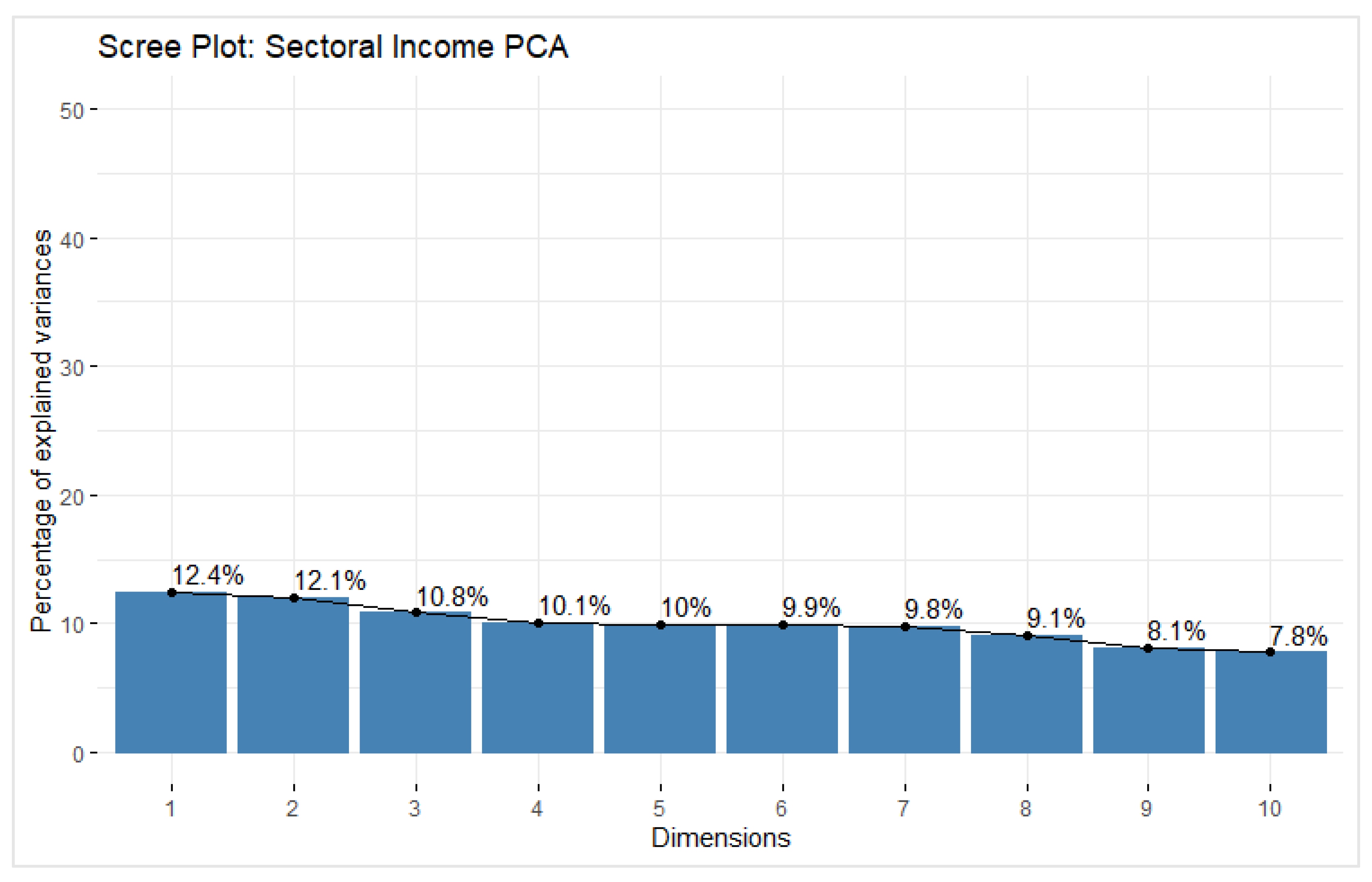
Figure 4.
Contribution Biplot for Dim-1-2.
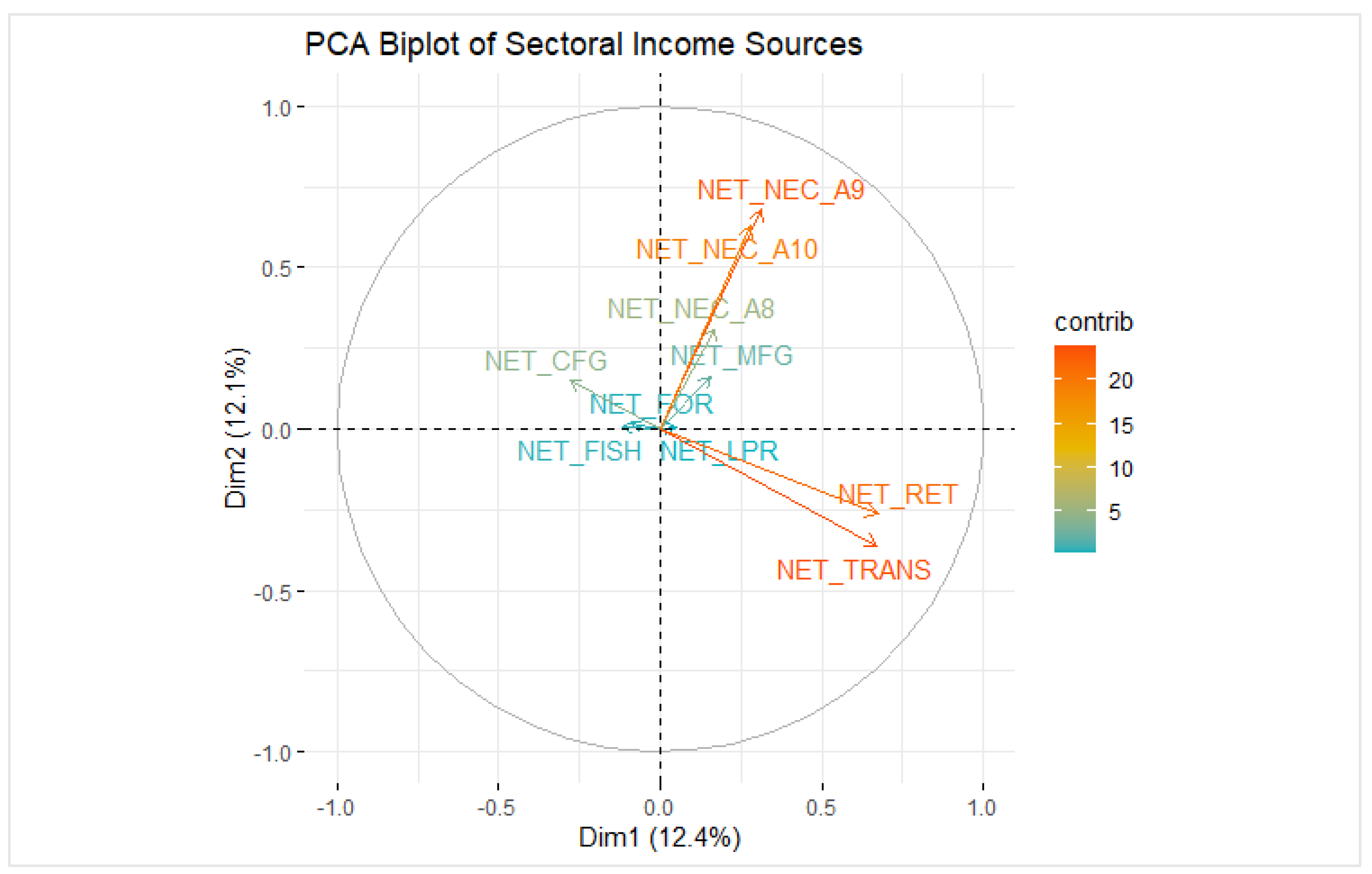
Figure 5.
Philippines Spatial Map for Mean Food Expenditure.
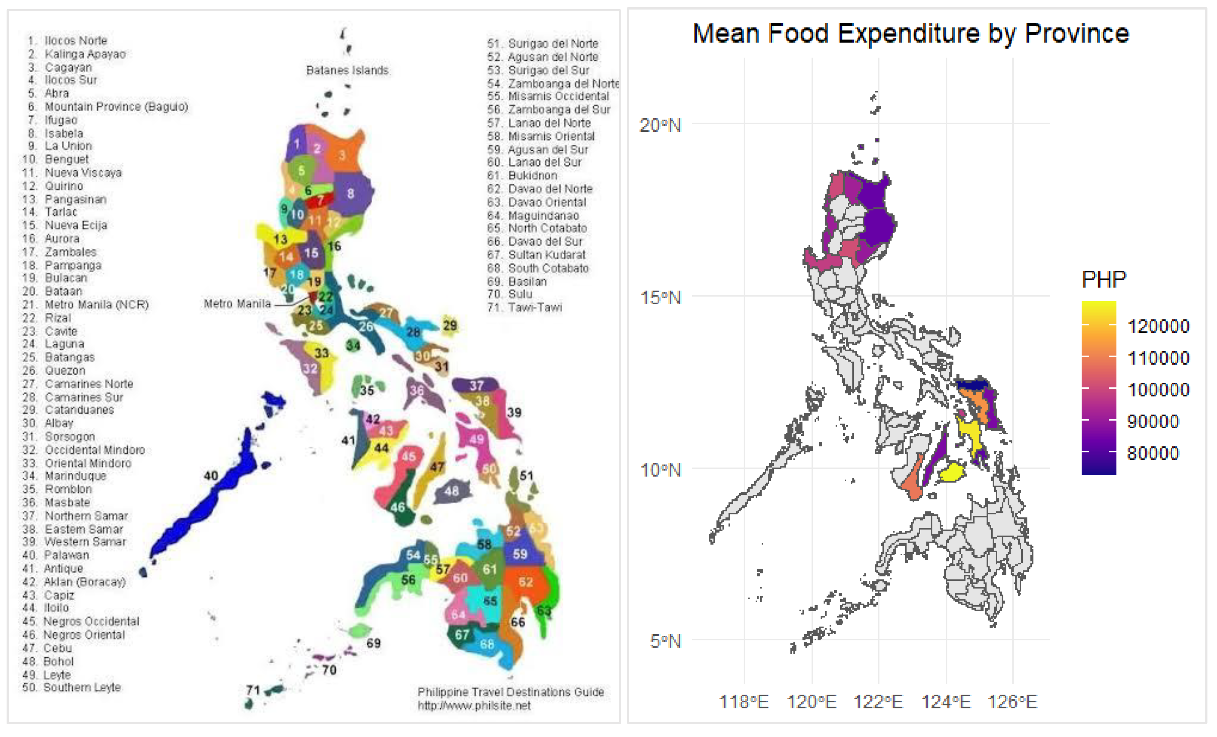
Figure 6.
Ternary Plot: Bread, Meat, and Fish Share of Total Food.
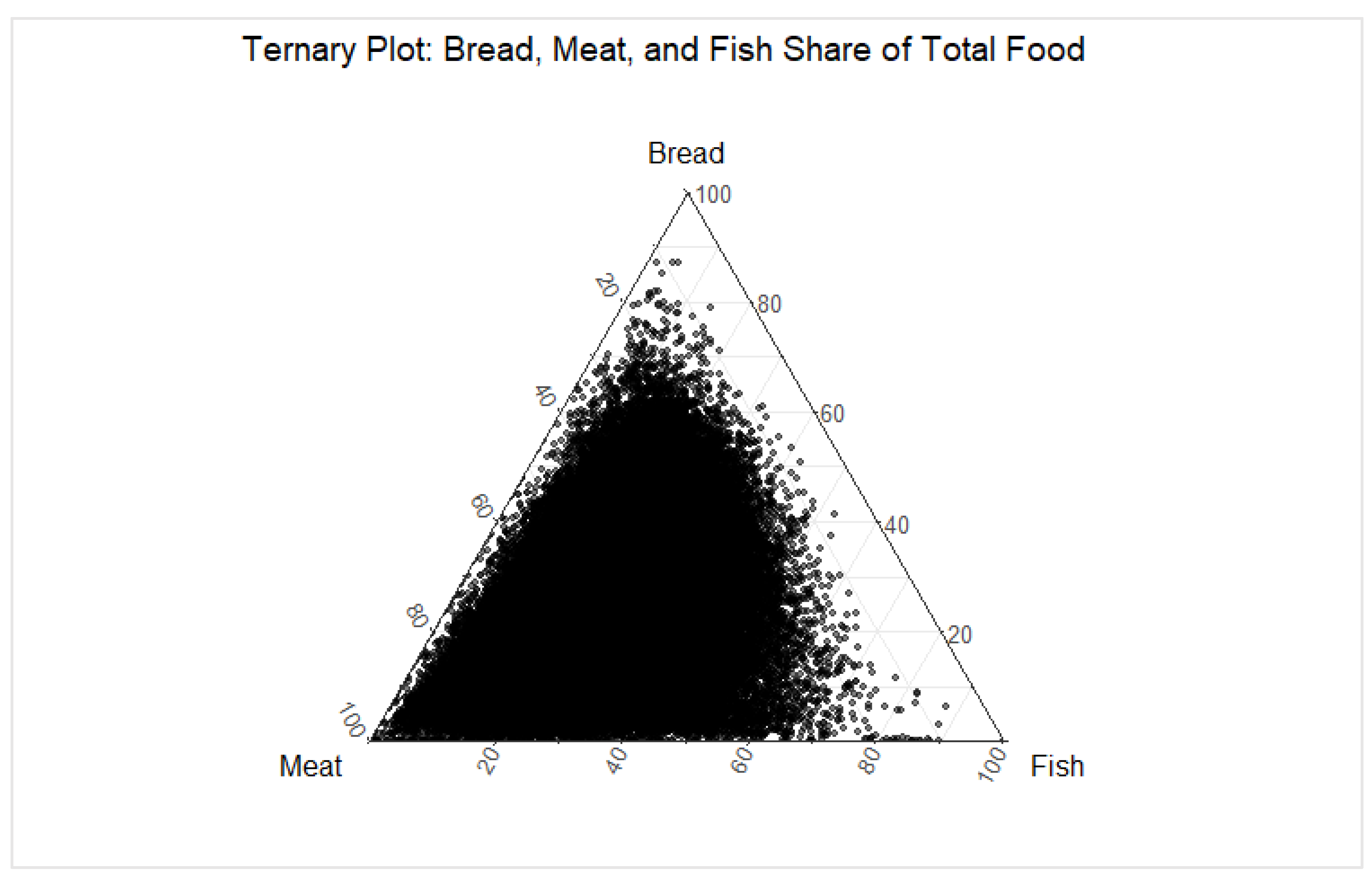
Figure 7.
Average Expenditure of Major Food Categories.
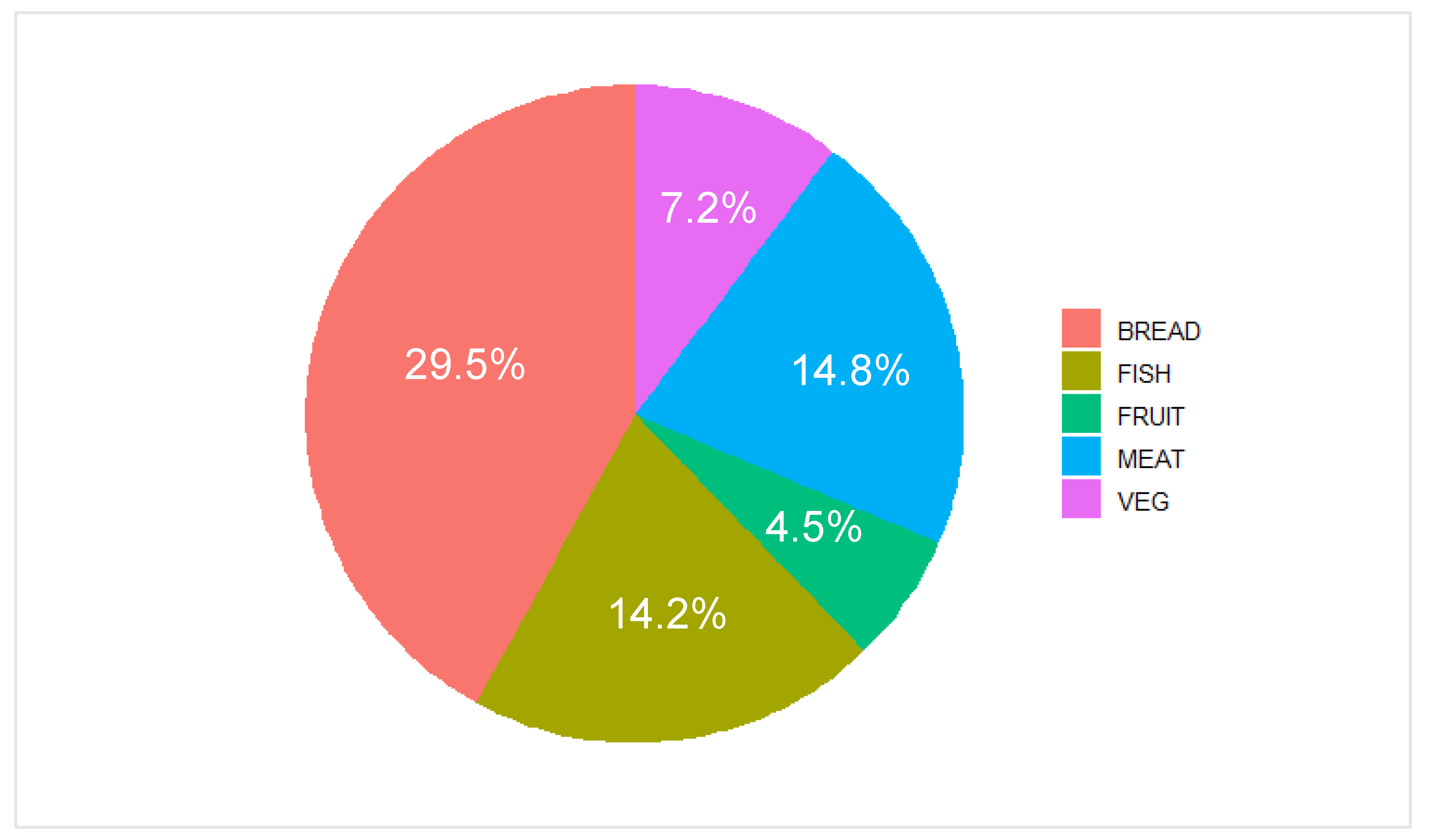
Figure 10.
Engel Curve (Log-Log): Relationship between Log of Total Income and Log of Food Expenditure among Filipino Households.
Figure 10.
Engel Curve (Log-Log): Relationship between Log of Total Income and Log of Food Expenditure among Filipino Households.
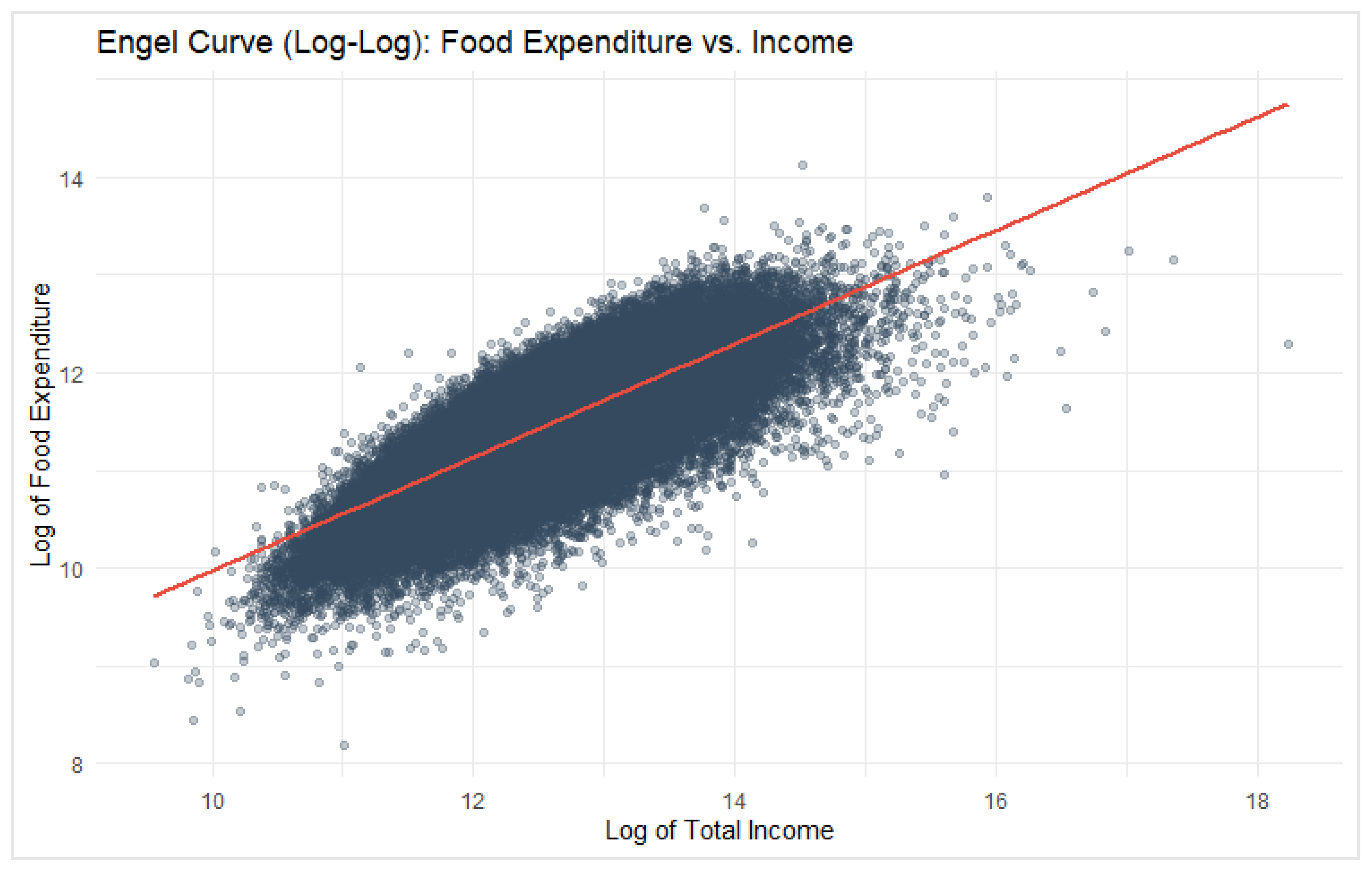
Table 1.
Descriptive Statistics.
| Metric | Value (Std. Error) |
| Mean Income | ₱332,147 (₱406,065.41) |
| Median Income | ₱241,080 |
| Mean Expenditure | ₱243,155 (₱193,120.45) |
| Mean Food Spending | ₱101,708 (₱69,317.68) |
| Mean RPCINC | ₱5.49 (₱5.01) |
| Mean Household Size | ~5.49 people (1.91) |
Table 2.
Gini Coefficients (Inequality Metrics).
| Variable | Gini Index | Qualitative Description |
| Total Income | 0.394 | Moderate inequality |
| RPCINC | 0.302 | Lower inequality (per capita adjusted) |
| Food Spending | 0.277 | Less inequality than income |
Table 3.
PCA Coordinates.
| Variable | PC1 | PC2 | PC3 | PC4 | PC5 |
| NET_CFG | -0.282 | 0.149 | 0.638 | 0.149 | 0.034 |
| NET_LPR | 0.053 | 0.006 | 0.373 | 0.426 | 0.610 |
| NET_FISH | -0.116 | 0.007 | -0.661 | 0.276 | 0.155 |
| NET_FOR | -0.092 | 0.015 | -0.033 | -0.762 | 0.575 |
| NET_RET | 0.675 | -0.265 | 0.091 | 0.042 | 0.110 |
| NET_MFG | 0.156 | 0.165 | -0.288 | 0.335 | 0.421 |
| NET_TRANS | 0.672 | -0.362 | 0.085 | -0.090 | -0.068 |
| NET_NEC_A8 | 0.170 | 0.310 | 0.039 | 0.073 | -0.273 |
| NET_NEC_A9 | 0.312 | 0.679 | 0.010 | -0.050 | -0.011 |
| NET_NEC_A10 | 0.279 | 0.631 | -0.013 | -0.127 | 0.013 |
Table 4.
Differences in Food and Income Between Rural and Urban Households.
| Variable | Group | Median | Wilcoxon W Statistic | p-value |
| FOOD | Rural | ₱102,467 | ||
| Urban | ₱80,700 | 4,237,060,363 | p<.001** | |
| RPCINC | Rural | ₱6,000 | ||
| Urban | ₱5,000 | 3,911,776,509 | p<.001** |
Note: * p < .001** (Highly Significant), p < .05* (Significant), p > .05 (Not significant).
Table 8.
Regression Results Predicting Food Expenditure from Total Income.
| Model | Predictor | (Estimate) | SE | t | p | R² |
| Linear Regression | Intercept | 77,880.00 | 148.90 | 523.0 | < .001 *** | 0.281 |
| Total Household Income | 0.072 | 0.00028 | 252.7 | < .001 *** | ||
| Log-Log Regression | Intercept | 4.177 | 0.01494 | 279.5 | < .001 *** | 0.589 |
| (Engel Curve) | Log Income | 0.580 | 0.00120 | 484.2 | < .001 *** |
Note. N = 163,268. SE = Standard Error; B = Unstandardized coefficient; R² = Coefficient of determination. **p < .001. The linear model estimates change in pesos; the log-log model estimates percentage changes (elasticity). SE=Standard error.
Table 9.
Empirical Rule of Thumb (based on Engel’s Law):.
| Income Elasticityof Food | Classification | Implication |
| Necessity Good | Food spending increases less than income | |
| Unit Elastic | Proportionate change | |
| Luxury Good | Food spending increases more than income |
Disclaimer/Publisher’s Note: The statements, opinions and data contained in all publications are solely those of the individual author(s) and contributor(s) and not of MDPI and/or the editor(s). MDPI and/or the editor(s) disclaim responsibility for any injury to people or property resulting from any ideas, methods, instructions or products referred to in the content. |
© 2025 by the authors. Licensee MDPI, Basel, Switzerland. This article is an open access article distributed under the terms and conditions of the Creative Commons Attribution (CC BY) license (http://creativecommons.org/licenses/by/4.0/).
Copyright: This open access article is published under a Creative Commons CC BY 4.0 license, which permit the free download, distribution, and reuse, provided that the author and preprint are cited in any reuse.


